Controlling roughening processes in the stochastic Kuramoto-Sivashinsky equation

Abstract

We present a novel control methodology to control the roughening processes of semilinear parabolic stochastic partial differential equations in one dimension, which we exemplify with the stochastic Kuramoto-Sivashinsky equation. The original equation is split into a linear stochastic and a nonlinear deterministic equation so that we can apply linear feedback control methods. Our control strategy is then based on two steps: first, stabilize the zero solution of the deterministic part and, second, control the roughness of the stochastic linear equation. We consider both periodic controls and point actuated ones, observing in all cases that the second moment of the solution evolves in time according to a power-law until it saturates at the desired controlled value.

1 Introduction

Roughening processes arise in nonequilibrium systems due to the presence of different mechanisms acting on multiple time and lengthscales and are typically characterized by a time-fluctuating “rough" interface whose dynamics are described in terms of a stochastic partial differential equation (SPDE). Examples are found in a broad range of different applications, including surface growth dynamics such as e.g. surface erosion by ion sputtering processes [9, 10], film deposition in electrochemistry [6, 7], or by other methods [22, 23],fluid flow in porous media [2, 45, 38], fracture dynamics [5] and thin film dynamics [27, 11, 36, 19, 4], to name but a few. Not surprisingly, understanding the dynamics of the fluctuating interface in terms of its roughening properties, which often exhibit scale-invariant universal features and long-range spatiotemporal correlations, has become an important problem in statistical physics which has received considerable attention over the last decades [3]. In addition, the ability of controlling not only the dynamics of the surface roughness (e.g.  its growth rate) but also its convergence towards a desired saturated value has recently received an increased interest due to its applicability in a wide spectrum of natural phenomena and technological applications.

Here we present a generic linear control methodology for controlling the surface roughness, i.e., the variance of the solution, of nonlinear SPDEs which we exemplify with the stochastic Kuramoto-Sivashinsky (sKS) equation. The starting point is to split the original SPDE into a stochastic linear part and a deterministic nonlinear part, and to apply existing control methodologies [16, 17] to the nonlinear deterministic part. Our control strategy is based on two steps: first, stabilize the zero solution of the deterministic system and, second, control the second moment of the solution of the stochastic linear equation (e.g. a measure of the surface roughness) to evolve towards any desired value. By considering either periodic or point actuated controls, our results show that the second moment of the solution grows in time according to a power-law with a well-defined growth exponent until it saturates to the prescribed value we wish to achieve.

It is important to note that other control strategies have been proposed previously for controlling the surface roughness and other quantities of interest, such as the film porosity and film thickness in various linear dissipative models, including the stochastic heat equation, the linear sKS equation, and the Edwards-Wilkinson (EW) equation; see e.g.  [22, 23, 24, 25, 32, 33, 34, 35, 48]. However, it should also be emphasized that most of these works involve the use of nonlinear feedback controls which change the dynamics of the system and require knowledge of the nonlinearity at all times, something that may be difficult to achieve. We believe that our framework offers several distinct advantages since the controls we derive and use are linear functions of the solution which do not affect the overall dynamics of the system and also decrease the computational cost. Another recent study is Ref.  [21] which considered a deterministic version of the KS equation, and presented a numerical study of the effects of the use of ion bombardment which varies periodically in time on the patterns induced by the ion beams on an amorphous material. In particular, this study found that rocking the material sample about an axis orthogonal to the surface normal and the incident ion beam, which corresponds to making the coefficients of the KS equation periodic in time, can lead to suppression of spatiotemporal chaos.

The work presented in this paper is motivated by earlier research carried out by our group: on one hand, the study of noise induced stabilization for the Kuramoto-Shivashinsky (KS) equation [40, 39] and, on the other hand, the study of optimal and feedback control methodologies for the KS equation and related equations that are used in the modeling of falling liquid films [16, 17, 46]. It was shown in [40, 39] that appropriately chosen noise can be used in order to suppress linear instabilities in the KS equation, close to the instability threshold. Furthermore, it was shown in [16, 17] that nontrivial steady states and unstable traveling wave solutions of the deterministic KS equation can be stabilized using appropriate optimal and feedback control methodologies. In addition, similar feedback control methodologies can be used in order to stabilize unstable solutions of related PDEs used in the modeling of falling liquid films, such the Benney and the weighted-residuals equations.

The rest of the paper is structured as follows. Section 2 introduces the sKS equation and discusses means to characterize the roughening process of its solution. In Section 3 we outline the general linear control methodology which is applied to the case of periodic controls in Section 4, and point actuated controls in Section 5. A summary and conclusions are included in Section 6.

2 The stochastic Kuramoto-Sivashinsky (sKS) equation

Consider the sKS equation:

$$u_{t}=-\nu u_{xxxx}-u_{xx}-uu_{x}+\sigma\xi(x,t),$$ (1)

normalized to $2\pi$ domains ($x\in[0,2\pi]$) with $\nu=(2\pi/L)^{2}>0$, where $L$ is the size of the system, with periodic boundary conditions (PBCs) and initial condition $u(x,0)=\phi(x)$. $\xi(x,t)$ denotes Gaussian mean-zero spatiotemporal noise, which is taken to be white in time, and whose strength is controlled by the parameter $\sigma$:

$$\left<\xi(x,t)\xi(x^{\prime},t^{\prime})\right>=\mathcal{G}(x-x^{\prime})\delta(t-t^{\prime}),$$ (2)

where $\mathcal{G}(x-x^{\prime})$ represents its spatial correlation function. We can, in principle, consider the control problem for SPDEs of the form (1) driven by noise that is colored in both space and time. Such a noise can be described using a linear stochastic PDE (Ornstein-Uhlenbeck process) [41].

The noise term can be expressed in terms of its Fourier components as:

$$\xi(x,t)=\sum_{k=-\infty}^{\infty}q_{k}\,\dot{W}_{k}(t)\,e^{ikx},$$ (3)

where $\dot{W}_{k}(t)$ is a Gaussian white noise in time and the coefficients $q_{k}$ are the eigenfunctions of the covariance operator of the noise. For example, if $\mathcal{G}(x-x^{\prime})=\delta(x-x^{\prime})$ (which corresponds to space-time white noise), we have $q_{k}=1$. For the noise to be real-valued, we require that the coefficients $q_{k}$ verify $q_{-k}=q_{k}$. Proofs of existence and uniqueness of solutions to Eq. (1) can be found in [12, 15], for example. The behavior of Eq. (1) as a function of the noise strength, and for particular choices of the coefficients $\{q_{k}\}$ has been analyzed in detail in [40, 39]. In particular, it was shown that sKS solutions undergo several state transitions as the noise strength increases, including critical on-off intermittency and stabilized states.

The quadratic nonlinearity in Eq. (1) is typically referred to as a Burgers nonlinearity. We note that an alternative version of Eq. (1) is found by making the change of variable $u=-h_{x}$, giving rise to

$$h_{t}=-\nu h_{xxxx}-h_{xx}+\frac{1}{2}(h_{x})^{2}+\sigma\eta(x,t),$$ (4)

where $\xi(x,t)=\partial_{x}\eta(x,t)$. The main effect of this transformation is to change the dynamics of the average $u_{0}(t)=\frac{1}{2\pi}\int_{0}^{2\pi}u(x,t)\,dx$ of the solution. Indeed, Eq. (1) with PBCs preserves the value of $u_{0}$ whereas as a consequence of the nonlinear term $(h_{x})^{2}$, Eq. (4) does not conserve the mass $h_{0}(t)=\frac{1}{2\pi}\int_{0}^{2\pi}h(x,t)\,dx$. Both equations have received a lot attention over the last decades, with Eq. (1) more appropriate in mass-conserved systems such as the dynamics of thin liquid films [39, 27, 11, 36, 19, 4], and Eq. (4) relevant in modeling surface growth processes such as surface erosion by ion sputtering processes [6, 7, 9, 10, 30, 33, 44]. It is also worth mentioning that the quadratic nonlinearity appearing in Eq. (4) is the same as that in the Kardar-Parisi-Zhang (KPZ) equation [28, 20]

$$h_{t}=h_{xx}+\frac{1}{2}(h_{x})^{2}+\sigma\eta(x,t).$$ (5)

In fact extensive work indicates that Eq. (4) and Eq. (5) are asymptotically equivalent, something referred to as the “Yakhot conjecture" [47, 42, 14]. Throughout the remainder of this study we will refer to Eq. (1) as the sKS equation with Burgers nonlinearity and Eq. (4) as the sKS equation with KPZ nonlinearity.

2.1 Surface roughening

An important feature of systems involving dynamics of rough surfaces is that one often observes the emergence of scale invariance both in time and space, i.e., the statistical properties of quantities of interest are described in terms of algebraic functions of the form $f(t)\sim t^{\beta}$ or $g(x)\sim x^{\alpha}$, where $\alpha$ and $\beta$ are referred to as scaling exponents. An example of this is the surface roughness, or variance of $u(x,t)$, which is defined as

$$r(t)=\sqrt{\frac{1}{2\pi}\int_{0}^{2\pi}\left[u(x,t)-u_{0}(t)\right]^{2}\ dx}.$$ (6)

We remark that $u_{0}$ may or may not depend on time, depending on whether we consider the Burgers or the KPZ nonlinearities. Usually the above quantity grows in time until it reaches a saturated regime, in which the fluctuations become statistically independent of time and are scale-invariant up to some typical length scale of the system, say $\ell_{s}$. This behavior can be expressed as:

$$\langle r(t)\rangle\sim\left\{\begin{array}[]{ll}t^{\beta}&\mathrm{if}\ \ t\ll t_{s},\\ r_{s}&\mathrm{if}\ \ t\gg t_{s},\end{array}\right.$$ (7)

where $\langle\dots\rangle$ denotes average over different realizations, $\beta$ is the so-called growth exponent [3], and $t_{s}$ and $r_{s}$ are the saturation time and saturated roughness value, respectively, which depend on the length scale $\ell_{s}$. In particular, at a given time $t<t_{s}$, the correlation of these fluctuations are on a spatial length scale which grows in time as $\ell_{c}\sim t^{1/z}$. Therefore, saturation occurs whenever $\ell_{c}=\ell_{s}$ from which we find $r_{s}\sim\ell_{s}^{\alpha}$ with $\alpha=\beta z$. In this context, the exponents $\alpha$ and $z$ are the roughness and dynamic exponent, respectively, and their particular values determine the type of universality class [29]. For example, it is known that the long-time behavior of the KPZ equation Eq. (5), is characterized by the KPZ universality class with $\alpha=1/2$ and $z=3/2$, while its linear version, which is referred to as the Edwards-Wilkinson (EW) equation, is characterized by the EW universality class with $\alpha=1/2$ and $z=2$ [3, 37, 8, 20].

Alternatively, the solution $u(x,t)$ can also be written in terms of its Fourier representation

$$u(x,t)=\sum_{k\in\mathbb{Z}}\hat{u}_{k}(t)e^{ikx},$$ (8)

where $\hat{u}_{k}(t)$ are the Fourier components. By making use of Parseval’s identity, we can compute the expected value of $r(t)^{2}$ as follows:

$$\left<r(t)^{2}\right>=\sum_{k\in\mathbb{Z}}\left<\left|\hat{u}_{k}(t)\right|^{2}\right>-\left<\left|u_{0}(t)\right|^{2}\right>=:\sum_{k\in\mathbb{Z}}S(k,t)-\left<\left|u_{0}(t)\right|^{2}\right>,$$ (9)

where we have defined the power spectral density $S(k,t)=\left<\left|\hat{u}_{k}(t)\right|^{2}\right>$. Therefore, if we can control the Fourier coefficients of the solution $u$, we can control the surface roughness to evolve to a desired target value $r_{d}$, i.e. $\mathrm{lim}_{t\to\infty}\sqrt{\left<r(t)^{2}\right>}=r_{d}$. In the following, we propose a control methodology precisely for this purpose.

3 Linear feedback control methodology

The methodology we propose to control the roughness of the sKS solution consists of two main steps. First,using a standard trick from the theory of semilinear parabolic SPDEs, see e.g. [15], we define $w$ to be the solution of the linear sKS equation:

$$w_{t}=-\nu w_{xxxx}-w_{xx}+\sigma\xi(x,t),$$ (10)

and write the full solution $u$ of Eq. (1) as $u=w+v$, so that $v$ satisfies

$$v_{t}=-\nu v_{xxxx}-v_{xx}-vv_{x}-(vw)_{x}-ww_{x}.$$ (11)

The important point here is to note that the above equation (11) is now a deterministic PDE with random coefficients and so we are in a position where we can apply the methodology for nonlinear deterministic PDEs we have developed in previous works [16, 17], to stabilize its zero solution - something possible as long as $w$ and its first derivative are bounded in an appropriate sense (see Section 4.2 below for a justification of this point). We therefore introduce the controlled equation for $v$:

$$v_{t}=-\nu v_{xxxx}-v_{xx}-vv_{x}-(vw)_{x}-ww_{x}+\sum_{n=-l_{1}}^{l_{1}}b^{det}_{n}(x)f^{det}_{n}(t),$$ (12)

where $m_{1}=1+2l_{1}$ (with $l_{1}=\left[1/\sqrt{\nu}\right]$) is the number of controls, and $b_{n}^{det}(x)$ are the control actuator functions. Here we use $\left[x\right]$ to denote the integer part of $x$.

Once the zero solution of the equation for $v$ has been stabilized, the second step is to control the roughness of the solution by applying appropriate controls to the linear SPDE (10) for $w$ so that the solution is driven towards the desired surface roughness $r_{d}$. In the following, we apply this methodology to the sKS equation, Eq. (1) or (4), by choosing two different types of controls, namely periodic controls, when the controls are applied throughout the whole domain and point actuated ones, when the control force is applied in a finite number of positions in the domain.

4 Periodic controls

4.1 Derivation of the controlled equation

From Eq. (12), we write

$$v(x,t)=\sum_{k\in\mathbb{Z}}\hat{v}_{k}(t)\,e^{ikx},$$ (13)

and take the inner product with the basis functions $e^{ikx}$ to obtain

$$\dot{\hat{v}}_{k}=\left(-\nu k^{4}+k^{2}\right)\hat{v}_{k}+g_{k}(v,w)+\sum_{n=-l_{1}}^{l_{1}}b^{det}_{nk}f^{det}_{n}(t),$$ (14)

with $k\in\mathbb{Z}$ and a dot denoting a time derivative. We have introduced $b_{nk}^{det}=\int_{0}^{2\pi}b_{n}(x)e^{ikx}dx$, and note that $g_{k}$ are functions of the coefficients of $v$ and $w$.

Next we define the following vectors and matrices. We denote the vector $z^{v}=[z_{s-}\ z_{un}^{v}\ z_{s+}^{v}]^{T}$, where $z_{un}^{v}=\left[v_{-l_{1}}\ \cdots\ v_{0}\ \cdots\ v_{l_{1}}\right]^{T}$ are the coefficients of the (slow) unstable modes, and $z_{s-}^{v}=\left[\cdots\ v_{-l_{1}-1}\right]^{T}$ and $z_{s+}^{v}=\left[v_{l_{1}+1}\ \cdots\right]^{T}$ are the coefficients of the (fast) stable modes. We also take $G=\left[\cdots\ g_{k}\ \cdots\right]^{T}$, $F^{det}=\left[f^{det}_{-l_{1}}(t)\ \cdots\ f^{det}_{l_{1}}(t)\right]^{T}$,

$$A=\left[\begin{array}[]{ccc}A_{s-}&0&0\\ 0&A_{u}&0\\ 0&0&A_{s+}\end{array}\right]\quad\textrm{ and }\quad B^{det}=\left[\begin{array}[]{c}B^{det}_{s-}\\ B^{det}_{u}\\ B^{det}_{s+}\end{array}\right],$$

where

$$A_{s-}=\operatorname{diag}(\cdots,-(l_{1}+1)^{4}\nu+(l_{1}+1)^{2},),$$

$$A_{u}=\operatorname{diag}(0,-(-l_{1})^{4}\nu+(-l_{1})^{2},\cdots,-l_{1}^{4}\nu+l_{1}^{2}),$$

$$A_{s+}=\operatorname{diag}(-(l_{1}+1)^{4}\nu+(l_{1}+1)^{2},\cdots),$$

and

$$B^{det}_{s-}=\left[\begin{array}[]{ccc}\vdots&\cdots&\vdots\\ b_{-l_{1}(-l_{1}-2)}^{det}&\cdots&b_{l_{1}(-l_{1}-2)}^{det,s}\\ b_{-l_{1}(-l_{1}-1)}^{det}&\cdots&b_{l_{1}(-l_{1}-1)}^{det,c}\end{array}\right],$$

$$B^{det}_{u}=\left[\begin{array}[]{ccc}b_{-l_{1}-l_{1}}^{det}&\cdots&b_{l_{1}-l_{1}}^{det}\\ \vdots&\cdots&\vdots\\ b_{l_{1}l_{1}}^{det}&\cdots&b_{l_{1}l_{1}}^{det}\end{array}\right],\quad B^{det}_{s+}=\left[\begin{array}[]{ccc}b_{-l_{1}(l_{1}+1)}^{det}&\cdots&b_{l_{1}(l_{1}+1)}^{det}\\ b_{-l_{1}(l_{1}+2)}^{det}&\cdots&b_{l_{1}(l_{1}+1)}^{det}\\ \vdots&\cdots&\vdots\end{array}\right].$$ (15)

With these definitions we rewrite the infinite system of ODEs (14) as

$$\dot{z}^{v}=Az^{v}+G+B^{det}F^{det}.$$ (16)

The key point now is to note that if there exists a matrix $K^{det}$ such that all the eigenvalues of the matrix $A_{u}+B^{det}_{u}K^{det}$ have negative real part, then the controls given by

$$f^{det}_{n}(t)=K^{det}_{n}z_{un}^{v}=K_{n}^{det}(z_{un}^{u}-z_{un}^{w}),$$ (17)

where $K^{det}_{n}$ is the $n-$th row of $K^{det}$, stabilize the zero solution of Eq. (12) (see [16, 17] for previously derived methodologies for deterministic systems). The proof of this follows the same type of Lyapunov argument as for the deterministic KS equation and is justified as long as we have nice bounds on $w$, something we will demonstrate below. It should be emphasized that in Eq. (16) for $v$ we have suppressed the influence of the nonlinearity on the SPDE without assuming knowledge of its value at all times and without changing the fundamental dynamics, in contrast to previous work [22, 23].

The next step is to control the stochastic linear equation for $w$ such that the value of the second moment evolves towards a desired target. To this end we write

$$w(x,t)=\sum_{k\in\mathbb{Z}}\hat{w}_{k}(t)e^{ikx},$$ (18)

and take the inner product with the basis functions to obtain the following infinite system of ODEs for the Fourier coefficients

$$\begin{array}[]{rcl}\dot{\hat{w}}_{0}&=&\xi_{0},\\ \dot{\hat{w}}_{k}&=&(-\nu k^{4}+k^{2})\hat{w}_{k}+\xi_{k}.\end{array}$$ (19)

Here $k\in\mathbb{Z}-\left\{0\right\}$, $\xi_{0}=\int_{0}^{2\pi}\xi(x,t)\,dx$, and $\xi_{k}=\int_{0}^{2\pi}\xi(x,t)e^{ikx}\,dx$. The solution to system (19) is

$$\begin{array}[]{rcl}\hat{w}_{0}(t)&=&\hat{w}_{0}(0)+\int_{0}^{t}\xi_{0}(t)\ dt,\\ \hat{w}_{k}(t)&=&e^{(-\nu k^{4}+k^{2})t}\hat{w}_{k}(0)+\int_{0}^{t}e^{(-\nu k^{4}+k^{2})(t-s)}\xi_{k}(s)\ ds,\end{array}$$ (20)

and it easily follows that

$$\left<\hat{w}_{k}(t)^{2}\right>=-\frac{\sigma^{2}}{2(-\nu k^{4}+k^{2})}(1-e^{-2(\nu k^{4}-k^{2})t}),\quad k\in\mathbb{Z}.$$ (21)

We observe that in this case the expected surface roughness only depends on the eigenvalues of the linear operator $\mathcal{L}=-\nu\partial_{x}^{4}-\partial_{x}^{2}$; these can be controlled using feedback control to direct the evolution towards the desired value of surface roughness $r_{d}$. Hence we introduce the controlled equation for $w$,

$$w_{t}=-\nu w_{xxxx}-w_{xx}+\sum_{n=-l_{2},n\neq 0}^{l_{2}}b^{rand}_{n}(x)f^{rand}_{n}(t)+\sigma\xi(x,t),$$ (22)

where $m_{2}=2l_{2}$ is the number of controls ($l_{2}$ needs to be larger than or equal to the number of unstable modes and will be specified later), and we choose the functions $b_{n}^{rand}(x)=e^{inx}$. We also notice that we do not need to control the eigenvalue corresponding to the constant eigenfunction ($k=0$), since it does not contribute to the surface roughness.

By truncating the system into $N$ modes (with $N$ sufficiently large so that the contribution from higher modes can be neglected) and taking inner products with the basis functions, we arrive at

$$\begin{array}[]{rclr}\dot{\hat{w}}_{0}&=&\xi_{0},\\ \dot{\hat{w}}_{k}&=&(-\nu k^{4}+k^{2})\hat{w}_{k}+f_{k}^{rand}+\xi_{k},\quad\ k=-l_{2},\dots,l_{2},\\ \dot{\hat{w}}_{k}&=&(-\nu k^{4}+k^{2})\hat{w}_{k}+\xi_{k},\quad\ k=-\frac{N}{2},\dots,-l_{2}-1,l_{2}+1,\dots,\frac{N}{2}.\end{array}$$ (26)

Remark 1.

An important point to note is that because of the choice of periodic functions for $b_{n}^{rand}$, the system (26) is decoupled. In fact, with such a choice of actuator functions, the matrix $B^{rand}_{u}$ is the identity matrix, and $B_{s\pm}^{rand}$ are zero matrices. As will be shown in Section 5, this is not the case for point actuated controls.

The surface roughness for $m_{2}=2l_{2}$ controls is therefore given by

$$\left<r^{2}(t)\right>=\sum_{k=-N/2,k\neq 0}^{N/2}\left<\hat{u}_{k}^{2}(t)\right>=\sum_{k=-l_{2},k\neq 0}^{l_{2}}\left<\hat{u}_{k}^{2}(t)\right>+\sum_{k=-N/2}^{-l_{2}-1}\left<\hat{u}_{k}^{2}(t)\right>+\sum_{k=l_{2}+1}^{N/2}\left<\hat{u}_{k}^{2}(t)\right>.$$

If we denote the desired surface roughness as $r_{d}^{2}=\mathrm{lim}_{t\to\infty}\left<r^{2}(t)\right>$, we obtain

$$\begin{array}[]{rl}r_{d}^{2}&=\sum_{k=-l_{2},k\neq 0}^{l_{2}}-\frac{\sigma^{2}|q_{k}|^{2}}{2\lambda_{k}}+\sum_{k=-N/2}^{-l_{2}-1}-\frac{\sigma^{2}|q_{k}|^{2}}{2(-\nu k^{4}+k^{2})}+\sum_{k=l_{2}+1}^{N/2}-\frac{\sigma^{2}|q_{k}|^{2}}{2(-\nu k^{4}+k^{2})}\\ &=-\frac{\sigma^{2}}{2}\sum_{k=-l_{2},k\neq 0}^{l_{2}}\frac{|q_{k}|^{2}}{\lambda_{k}}+\underbrace{\sigma^{2}\sum_{k=l_{2}+1}^{N/2}-\frac{|q_{k}|^{2}}{-\nu k^{4}+k^{2}}}_{\left<r_{f}^{2}\right>},\end{array}$$

where we have used the fact that the coefficients $q_{k}$ are real with $q_{-k}=q_{k}$ (see equation (3)). The chosen eigenvalues for the controlled modes are $\lambda_{k}$, and we take them to be $\lambda_{k}=\lambda$ for all $k$ to arrive at

$$\lambda=-\frac{\sigma^{2}\sum_{k=1}^{l_{2}}|q_{k}|^{2}}{\left<r_{d}^{2}\right>-\left<r_{f}^{2}\right>}.$$ (27)

To control the surface roughness we therefore define the controls $f^{rand}_{k}$ such that the new eigenvalues satisfy the following relation

$$f^{rand}_{k}=\left(\lambda+\nu k^{4}-k^{2}\right)\hat{w}_{k}.$$ (28)

Finally, putting Eqs. (12) and (22) together, yields the controlled equation for the full solution $u$

$$u_{t}=-\nu u_{xxxx}-u_{xx}-uu_{x}+\xi(x,t)+\sum_{n=-l_{1}}^{l_{1}}b^{det}_{n}(x)f_{n}^{det}(t)+\sum_{n=-l_{2}}^{l_{2}}b^{rand}_{n}(x)f_{n}^{rand}(t).$$ (29)

4.2 Proof of applicability of the control methodology

Our aim here is to prove that the solution $v$ can indeed be controlled to zero even though Eq. (12) has random coefficients, i.e. the terms $(vw)_{x}$ and $ww_{x}$. We will show that by adopting a similar argument as used for the proof of existence and uniqueness of solutions of the sKS equation [15], we can apply a Lyapunov-type argument as in the deterministic KS equation [17].

We use (28) to write the solution of Eq. (22) as

$$w(t)=e^{\mathcal{A}t}w(x,0)+\sigma\int_{0}^{t}e^{\mathcal{A}(t-s)}d\xi(s),$$

where $\mathcal{A}=-(\nu A^{2}-A+F)$, $A=-\partial_{x}^{2}$ and $F$ is an operator discretised as

$$F=\left[\begin{array}[]{ccc}0&0&0\\ 0&\operatorname{diag}(\lambda-\nu k^{4}+k^{2})&0\\ 0&0&0\end{array}\right].$$

We take $\mathcal{G}$ to be a trace class operator, so that it satisfies [15, Assumption (3.1)]. Writing

$$e^{\mathcal{A}(t-s)}\xi(s)=\sigma\sum_{j,k\in\mathbb{Z}}q_{k}\,e^{-(\nu k^{4}-k^{2}+f_{k})(t-s)}<e_{k},e_{j}>\beta_{k}(s)e_{j},$$

we have

$$\mathbb{E}[w(t)] =e^{\mathcal{A}t}w(x,0)=0,$$ (30a)

$$\mathbb{E}[|w(t)-\mathbb{E}[w(t)]|^{2}] =\sigma^{2}\sum_{j,k\in\mathbb{Z}}\int_{0}^{t}e^{-2(\nu k^{4}-k^{2}+f_{k})(t-s)}|q_{k}|^{2}\,|<e_{k},e_{j}>|^{2},$$

$$=\sum_{k=-l_{2}}^{l_{2}}\frac{\sigma^{2}|q_{k}|^{2}}{\lambda}+\sum_{|k|\geq l_{2}}\frac{\sigma^{2}|q_{k}|^{2}}{2(\nu k^{4}-k^{2})}=r_{d}^{2},$$ (30b)

where we used $<e_{k},e_{j}>=0$ and $f_{k}=\lambda+\nu k^{4}-k^{2}$. Since we are assuming that the covariance matrix $G$ is such that assumption (3.1) in [15] is satisfied, we have that $w(t)\in\dot{L}^{2}(0,2\pi)$, the space of mean zero $L^{2}$ functions, almost surely, for any time $t$. This also means [41] that there exists a continuous version of $w$ that we shall consider from now on.

Now we define $B(u,v)=uv_{x}$ and $b(u,v,w)=<B(u,v),w>=\int_{0}^{2\pi}uv_{x}w\ dx$, which satisfy the following relations [15, 43]:

$$\|b(u_{1},u_{2},u_{3})\|_{L^{2}} \leq\|u_{1}\|_{L^{2}}\|u_{2,x}\|_{L^{\infty}}\|u_{3}\|_{L^{2}}\leq c\|u_{1}\|_{L^{2}}\|Au_{2}\|_{L^{2}}\|u_{3}\|_{L^{2}},$$ (31a)

$$b(u,u,u) =0,$$ (31b)

$$b(u_{1},u_{2},u_{2}) =b(u_{2},u_{2},u_{1})=-\frac{1}{2}b(u_{2},u_{1},u_{2}),$$ (31c)

$$b(u_{1},u_{2},u_{3}) =-b(u_{2},u_{1},u_{3})-b(u_{1},u_{3},u_{2}).$$ (31d)

and [15, Proposition (2.1)]:

$$\|B(u,v)\|_{D(A^{-1})} \leq c\|Au\|_{L^{2}}\|v\|_{L^{2}},$$ (32a)

$$\|B(z,v)\|_{D(A^{-1})} \leq c\|u\|_{L^{2}}\|Av\|_{L^{2}},$$ (32b)

$$\|B(z,z)\|_{D(A^{-1})} \leq c\|z\|_{L^{2}}^{2},$$ (32c)

$$\|B(u,v)\|_{D(A^{-\delta})} \leq c\|u\|_{D(A^{\frac{1}{2}-\delta})}\|v\|_{D(A^{\frac{1}{2}-\delta})}.$$ (32d)

On the other hand, we notice that the existence of the matrix $K^{det}$ implies that the operator $\mathcal{A}$, such that $\mathcal{A}v=-\nu v_{xxxx}-v_{xx}-\sum_{n=-l_{1}}^{l_{1}}b_{n}^{det}(x)f_{n}^{det}(t)$, satisfies

$$\int_{0}^{2\pi}v\mathcal{A}v\ dx\leq-a\|v\|_{L^{2}}^{2},$$ (33)

for some positive constant $a$, which in turn depends on the eigenvalues we choose for the controlled operator. Therefore, multiplying equation (12) by $v$ and integrating by parts yields

$$\frac{1}{2}\frac{d}{dt}\|v\|_{L^{2}}^{2}\leq-a\|v\|_{L^{2}}^{2}-\overbrace{b(v,v,v)}^{=0}-b(v,w,v)-b(v,w,v)-b(w,w,v)\\ =-a\|v\|_{L^{2}}^{2}+b(w,v,v)+\frac{1}{2}b(w,v,w)\leq-a\|v\|_{L^{2}}^{2}+c\|w\|_{L^{2}}\|v\|_{L^{2}}\|Av\|_{L^{2}}\\ +\frac{c}{2}\|w\|_{L^{2}}^{2}\|Av\|_{L^{2}}\leq-\left(a-\frac{c}{2}\|w\|_{L^{2}}^{2}\right)\|v\|_{L^{2}}^{2}+c\|Av\|_{L^{2}}^{2}+\frac{c}{2}\|w\|_{L^{2}}^{4},$$ (34)

where we have used Young’s inequality and relations (31) and (32). The term $c\|Av\|_{L^{2}}^{2}$ can be controlled using sufficiently strong controls and the last term on the right-hand-side is a constant that depends on the desired surface roughness and that again can be controlled by choosing large enough eigenvalues. Therefore, by choosing the controls such that $a$ is large enough, $\|v\|^{2}_{L^{2}}$ is a Lyapunov function for this system and the zero solution for the controlled equation for $v$ is stable.

4.3 Numerical results

We apply now the methodology presented above with periodic controls to the sKS with either the Burgers nonlinearity (Eq. (1)) or the KPZ nonlinearity (Eq. (4)). For simplicity, we consider white noise in both space and time ($q_{k}=1$). All our numerical experiments are solved using spectral methods in space and a second-order backward differentiation formula scheme in time  [1].

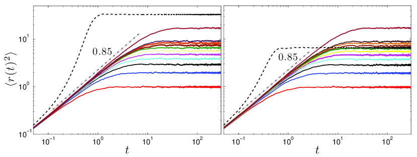
Figure 1: Squared value of the surface roughness of the solutions to the sKS equation with Burgers nonlinearity (left) and the KPZ nonlinearity (right) for $\nu=0.05$, $\sigma=0.5$ and different values of the desired surface roughness, ranging from $1$ to $10$, and $20$. The dashed lines show the value of the uncontrolled roughness, and the straight dashed-line corresponds to a guide-to-eye line with slope $0.85$.

4.3.1 Controlling the roughening process

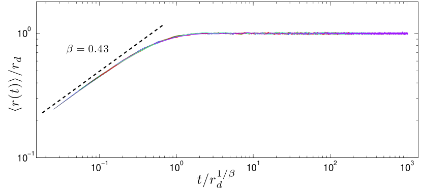
Figure 2: Surface roughness rescaled by the target value $r_{d}$ against the rescaled time $t/r_{d}^{1/\beta}$ for all cases shown in Fig. 1. The dashed line corresponds to a guide-to-eye line with slope $0.43$.

We solved Eqs. (1) and (4) for $\nu=0.05$ and $\sigma=0.5$, controlling its solutions towards various desired surface roughnesses $r_{d}$. The results are presented in Fig. 1. We observe that in both cases the solution exhibits a power-law behavior at short times of the form given by Eq. (7) until the solution saturates to the desired value of the roughness. It is interesting to note that the exponent in all cases is the same with $\beta\approx 0.43$, independently of the type of nonlinearity and desired surface roughness (note that the exponent in Fig.1 is $\approx 0.85=2\beta$, since we are plotting $<r(t)^{2}>$). This becomes even clearer if time and surface roughness are rescaled by their saturation values, $t_{s}$ and $r_{d}$, respectively. By noting that $r_{d}\sim t_{s}^{\beta}$, Eq. (7) is rewritten as:

$$\frac{\langle r(t)\rangle}{r_{d}}\sim\left\{\begin{array}[]{ll}x^{\beta}&\mathrm{if}\ \ x\ll 1,\\ 1&\mathrm{if}\ \ x\gg 1,\end{array}\right.$$ (35)

where $x=t/r_{d}^{1/\beta}$. Fig. 2 shows that all the different cases presented in Fig. 1 collapse into a single curve which is given by (35) above with the universal value $\beta\approx 0.43$.

We also study the effect of changing the domain by varying the parameter $\nu$. Fig. 3 shows the numerical results obtained when we fix the target value $r_{d}$ and change the parameter $\nu$. We observe that changing the domain does not change the growth rate (we observe the same growth exponent $\beta\approx 0.43$) but it does slightly affect the final value of the roughness. An important point to note is that since we are controlling the surface roughness of the solution $r(t)$ to be at a specified value $r_{d}$, the saturated state in which the statistical properties become stationary, is reached whenever $r(t)=r_{d}$. Therefore, the saturation time, and the long-time roughness value, should not depend on the system size.

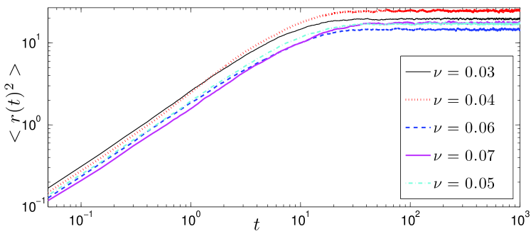
Figure 3: Controlled roughness with same target value $r_{d}^{2}=20$ and different values of $\nu$ - the domain size increases as $\nu$ decreases.

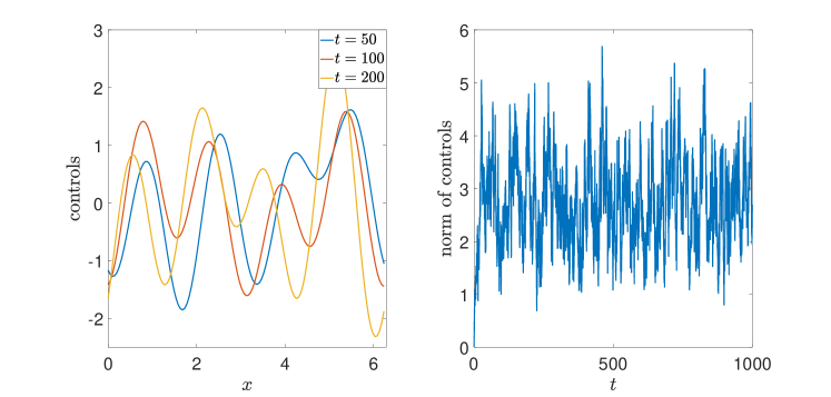
Figure 4: Left: Controls at different time steps. Right: $L^{2}$-norm of the controls as a function of time. For both figures $\nu=0.05$ and $\sigma=0.5$.

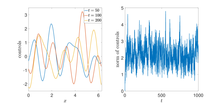
Figure 5: Left: Controls at different time steps. Right: $L^{2}$-norm of the controls as a function of time. For both figures $\nu=0.03$ and $\sigma=0.5$.

4.3.2 Changing the shape of the solution

It is important to emphasize that in addition to controlling the roughness of the solution of the sKS equation, we can also change its shape, something that could have ramifications in technological applications such as materials processing. We quantify this by considering the surface roughness of the solution as is its distance to the desired state. If $\bar{u}(x)$ is the ultimate desired shape of the solution, then the quantity we are trying to control now becomes

$$r(t)=\sqrt{\frac{1}{2\pi}\int_{0}^{2\pi}\left(u(x,t)-\bar{u}\right)^{2}\ dx}.$$ (36)

Using Parseval’s identity we compute the expected value of $r(t)^{2}$

$$\left<r(t)^{2}\right>=\sum_{k\in\mathbb{Z},k\neq 0}\left<\left(u_{k}(t)-\bar{u}_{k}\right)^{2}\right>.$$ (37)

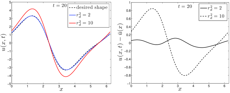
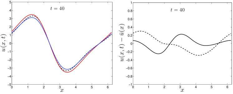
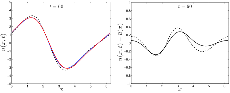
Figure 6: Snapshots of the sKS equation solution controlled to the shape of one of the steady states of the KS equation (left panels) and difference between current solution and desired shape for two different desired surface roughness (right panels). Parameters are $\nu=0.5$, $\sigma=0.5$, $r_{d}^{2}=2$ (blue) and $r_{d}^{2}=10$ (red) with $T=100$ and $dt=5\times 10^{-3}$.

To control the shape of the solution, we can therefore control the solution of equation (12) for $v$ to the desired shape rather than controlling it to zero. This in turn implies the use of $f^{det}_{n}(t)=K^{det}_{n}\left(z_{un}^{v}-z_{un}^{\bar{u}}\right)=K_{n}^{det}(z_{un}^{u}-z_{un}^{w}-z_{un}^{\bar{u}})$. We use the steady states of the KS equation for a chosen value of $\nu$ to define the desired shape $\bar{u}$. Results are shown in Fig. 6 for $\nu=0.5$, where we can see that the solution is fluctuating around the imposed shape.

5 Point actuated controls

We now consider controls that are point actuated and not distributed throughout the whole domain, i.e. the functions $b_{n}(x)$ are now given by $b_{n}(x)=\delta(x-x_{n})$, where $\delta(x)$ is the Dirac delta function. By repeating the same procedure as with periodic controls, writing $w=\sum_{k\in\mathbb{Z}}\hat{w}_{k}e^{ikz}$ and taking the inner product with the eigenfunctions of the linear operator, $\mathcal{L}=-\nu\partial_{x}^{4}-\partial_{x}^{2}$, we obtain the following infinite system of linear stochastic ODEs

$$\begin{array}[]{rclr}\dot{\hat{w}}_{0}&=&\xi_{0}+\sum_{n=1}^{m}b_{n}^{0}f_{n},&\\ \dot{\hat{w}}_{k}&=&(-\nu k^{4}+k^{2})\hat{w}_{k}++\sum_{n=1}^{m_{2}}b_{n}^{k}f_{n}+\xi_{k},&k\neq 0,\end{array}$$ (38)

where the coefficients $b_{n}^{k}$ are defined from the functions $b(x)=\delta(x-x_{n})$ as before, $b_{n}^{k}=\int_{0}^{2\pi}b_{n}(x)e^{ikx}dx$. We can see that the difference between the above system and the periodic controls one given by (26), is that now the system is coupled. In fact the coupling matrix is not symmetric, and most importantly, it does not commute with its transpose. Therefore the solution does not follow directly and we cannot easily write the second moment of the coefficients as a function of the eigenvalues as in the previous section. To obtain the controlled equation we thus need to apply a different approach.

Let the controls $F=[f_{1},\cdots,f_{m}]$ be such that $F=K\hat{w}$ where $\hat{w}$ is a vector containing the Fourier coefficients of $w$, and the matrix $K$ is to be determined. Since the equations are not decoupled we cannot multiply by $w$ and integrate to find directly the second moment of the coefficients. However, we can make use of results derived in [26] which provide simplified formulas for the first and second moments of systems analogous to (38). Let $\Xi$ be the vector $\Xi_{k}=\xi_{k}$ and $C=A+BK$ where $A=\operatorname{diag}-\nu k^{4}+k^{2}$ and $B_{kn}=b_{n}^{k}$, so that we can write the truncated system (26) as

$$\dot{\hat{w}}=A\hat{w}+BK\hat{w}+\Xi:=C\hat{w}+\Xi.$$

We also assume without loss of generality that $\mathbf{m}(0)=\mathbb{E}(\hat{w}(0))=0$ and $\mathbf{P}(0)=\mathbb{E}(\hat{w}(0)\hat{w}(0)^{T})=0$. Then Theorem $4$ in [26] states that

$$\mathbf{m}(t)=\mathbb{E}(\hat{w}(t))=0\quad\text{ and }\quad\mathbf{P}(t)=\mathbb{E}(\hat{w}(t)\hat{w}(t)^{T})=\mathbf{H}_{1}\mathbf{F}_{1}^{T}+\mathbf{F}_{1}\mathbf{H}_{1}^{T}$$

where $\mathbf{F_{1}}$ and $\mathbf{H_{1}}$ are the $(1,1)$ and $(1,3)$ blocks of the matrix $e^{Mt}$ where in the case of space-time white noise, $M$ is

$$M=\left[\begin{array}[]{cccc}C&0&\frac{\sigma^{2}}{2}I&0\\ 0&0&0&0\\ 0&0&-C^{T}&0\\ 0&0&0&0\end{array}\right],$$

$I$ is an appropriately sized identity matrix and the zeros stand for zero matrices of appropriate size. We compute $e^{Mt}$ and conclude that

$$\mathbf{F}_{1}=e^{Ct},$$

and

$$\mathbf{H}_{1}= \frac{\sigma^{2}}{2}\left[It+(C-C^{T})\frac{t^{2}}{2}+(C^{2}-CC^{T}+(C^{T})^{2})\frac{t^{3}}{3!}\right]$$

$$+\frac{\sigma^{2}}{2}\left[(C^{3}-C^{2}C^{T}+C(C^{T})^{2}-(C^{T})^{3})\frac{t^{4}}{4!}+\cdots\right].$$

Since $\mathbf{F}_{1}\mathbf{H}_{1}^{T}=(\mathbf{H}_{1}\mathbf{F}_{1}^{T})^{T}$ and $(\mathbf{H}_{1}\mathbf{F}_{1}^{T})^{T}=\mathbf{H}_{1}\mathbf{F}_{1}^{T}$, we have $\mathbf{H}_{1}\mathbf{F}_{1}^{T}+\mathbf{F}_{1}\mathbf{H}_{1}^{T}=2\mathbf{H}_{1}\mathbf{F}_{1}^{T}$, from which we obtain

$$\mathbf{P}(t)=\sigma^{2}\left(It+(C+C^{T})\frac{t^{2}}{2}+\left(C^{2}+2CC^{T}+(C^{T})^{2}\right)\frac{t^{3}}{3!}+\right.\\ +\left(C^{3}+3C^{2}C^{T}+3C(C^{T})^{2}+(C^{T})^{3}\right)\frac{t^{4}}{4!}+\\ \left.+\left(C^{4}+4C^{3}C^{T}+6C^{2}(C^{T})^{2}+4C(C^{T})^{3}+(C^{T})^{4}\right)\frac{t^{5}}{5!}+\cdots\right).$$ (39)

Remark 2.

In the periodic case, the matrix $C$ is diagonal, so $CC^{T}=C^{T}C$, and this is exactly the same as

$$\mathbf{P}(t)=\sigma^{2}\sum_{n=1}^{\infty}\left(C+C^{T}\right)^{n-1}\frac{t^{n}}{n!}.$$ (40)

In addition, when choosing the eigenvalues of $C$, we can ensure that it is invertible and therefore $C+C^{T}$ is also invertible, which gives

$$\mathbf{P}(t)=-\sigma^{2}\left(C+C^{T}\right)^{-1}+\sigma^{2}e^{(C+C^{T})t},$$ (41)

so as $t\rightarrow\infty$, $\mathbf{P}(t)\rightarrow-\sigma^{2}\left(C+C^{T}\right)^{-1}$ and

$$<r(t)^{2}>=\operatorname{tr}(\mathbf{P}(t))\rightarrow\sum_{k\in{\mathbb{Z}-\left\{0\right\}}}-\frac{\sigma^{2}}{2\lambda_{k}},$$ (42)

where $\lambda_{k}$ are the chosen eigenvalues of $C$. Hence we recover the same result as before.

It is important to note that the matrix $C$ is not normal, i.e. it does not commute with its transpose, and the eigenvalues of $C+C^{T}$ do not satisfy the useful properties that allow us to obtain (30). However, we are not interested in knowing the full matrix $\mathbf{P}(t)$, but only its trace

$$\operatorname{tr}(\mathbf{P}(t))=\operatorname{tr}\left(\sigma^{2}\left(It+(C+C^{T})\frac{t^{2}}{2}+\left(C^{2}+2CC^{T}+(C^{T})^{2}\right)\frac{t^{3}}{3!}+\right.\right.\\ +\left(C^{3}+3C^{2}C^{T}+3C(C^{T})^{2}+(C^{T})^{3}\right)\frac{t^{4}}{4!}+\\ \left.\left.+\left(C^{4}+4C^{3}C^{T}+6C^{2}(C^{T})^{2}+4C(C^{T})^{3}+(C^{T})^{4}\right)\frac{t^{5}}{5!}+\cdots\right)\right).$$ (43)

By now making use of the linearity of the trace and its continuity to pass it inside the infinite sum, we get

$$\operatorname{tr}(\mathbf{P}(t))=\sigma^{2}\left(\operatorname{tr}(I)t+\operatorname{tr}(C+C^{T})\frac{t^{2}}{2}+\operatorname{tr}\left(C^{2}+2CC^{T}+(C^{T})^{2}\right)\frac{t^{3}}{3!}+\right.\\ +\operatorname{tr}\left(C^{3}+3C^{2}C^{T}+3C(C^{T})^{2}+(C^{T})^{3}\right)\frac{t^{4}}{4!}+\\ \left.+\operatorname{tr}\left(C^{4}+4C^{3}C^{T}+6C^{2}(C^{T})^{2}+4C(C^{T})^{3}+(C^{T})^{4}\right)\frac{t^{5}}{5!}+\cdots\right).$$ (44)

We also note that

$$\operatorname{tr}\left(C^{2}+2CC^{T}+(C^{T})^{2}\right)=\operatorname{tr}\left(C^{2}+CC^{T}+C^{T}C+(C^{T})^{2}\right)=\operatorname{tr}(C+C^{T})^{2}.$$

Similarly we can prove that the terms multiplied by $\frac{t^{n}}{n!}$ are of the form $\operatorname{tr}\left((C+C^{T})^{n-1}\right)$ and we finally obtain

$$\operatorname{tr}(\mathbf{P}(t))=\sigma^{2}\left(\operatorname{tr}(I)t+\operatorname{tr}(C+C^{T})\frac{t^{2}}{2}+\operatorname{tr}\left(C+C^{T}\right)^{2}\frac{t^{3}}{3!}+\right.\\ \left.+\operatorname{tr}\left(C+C^{T}\right)^{3}\frac{t^{4}}{4!}+\operatorname{tr}\left(C+C^{T}\right)^{4}\frac{t^{5}}{5!}+\cdots\right).$$ (45)

We proceed by assuming that $C+C^{T}$ is invertible, so that we can multiply by $I=(C+C^{T})^{-1}(C+C^{T})$ and add and subtract pertinent terms to obtain

$$\operatorname{tr}(\mathbf{P}(t))=-\sigma^{2}\operatorname{tr}\left(C+C^{T}\right)^{-1}+\sigma^{2}\operatorname{tr}\left(\left(C+C^{T}\right)^{-1}\sum_{n\in\mathbb{N}}\left(C+C^{T}\right)^{n}\frac{t^{n}}{n!}\right).$$ (46)

Remark 3.

This does not change the proof provided in Section 4.2, it only changes the formula for the covariance so that the bounds are still valid.

Remark 4.

We emphasize that the following assumptions were made here:

• $C+C^{T}$ needs to be invertible.

• In order for the surface roughness to converge to a finite value, we require all of the eigenvalues of $C+C^{T}$ to be negative, so that the exponential part disappears.

5.1 Computation of the matrix $K$

We note in Eq. (46) that we now need to control the trace of $D^{-1}=(C+C^{T})^{-1}$ and we can do that by prescribing the eigenvalues of $D$. Hence we can control the surface roughness by finding a matrix $K$ such that the eigenvalues of

$$D=C+C^{T}=A+BK+A^{T}+(BK)^{T}=2A+BK+K^{T}B^{T},$$ (47)

are a given set $\left\{\mu_{1},\dots,\mu_{N}\right\}$. Since we only wish to prescribe the eigenvalues of $D$, rather than knowing all of its entries, we can tackle this problem by using the information provided by the characteristic polynomial, $\chi_{D}$, of $D$. We know that

$$\chi_{D}(t)=\prod_{i=1}^{N}(t-\mu_{i})=\sum_{k=0}^{N}(-1)^{k}\sum_{J:|J|=k}\prod_{j\in J}\mu_{j}t^{N-k},$$ (48)

where $J$ is a subset of $\left\{1,\dots,N\right\}$. Equivalently we can express $\chi_{D}$ in terms of the sum over all its diagonal minors, i.e.,

$$\chi_{D}=\sum_{k=0}^{N}(-1)^{k}\,\eta_{k}\,t^{N-k},$$ (49)

where $\eta_{k}$ is the sum over all of the diagonal minors of size $k$ of $D$. This translates into a system of $N$ nonlinear algebraic equations,

$$\eta_{k}=\sum_{J:|J|=k}\prod_{j\in J}\mu_{j},$$

for the $m\times N$ entries of the matrix $K$ - see [18] for details on the solution to this problem. For the purposes of our study, we will make use a nonlinear solver (e.g., Matlab’s fsolve) to obtain the matrix $K$. Given the structure of the matrix $B$ and the fact that the system is underdetermined, convergence is rather slow when solving the problem directly. We overcome this by performing a change of variables: we obtain the SVD decomposition of $B$ by finding matrices $X$ and $Y$ such that $\tilde{B}=XBY^{T}$, and multiply equation (47) by $X^{T}$ on the left and by $X$ on the right. We then define $\tilde{K}=Y^{T}KX$, $\tilde{A}=X^{T}AX$ and $\tilde{D}=X^{T}DX$, so that we obtain the equation

$$\tilde{D}=2\tilde{A}+\tilde{B}\tilde{K}+\tilde{K}^{T}\tilde{B}^{T}.$$ (50)

This is of the same form as (47), but where the matrix $\tilde{B}$ is diagonal. We find that this accelerates the convergence of the system (for moderate values of $N$) and we were able to get satisfactory numerical results, which we now present.

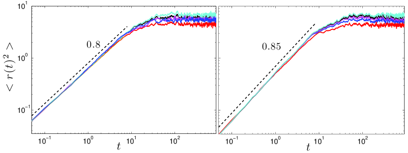
Figure 7: Squared value of the surface roughness of the solutions to the sKS equation with Burgers nonlinearity for $\nu=0.04$, $\sigma=0.5$ and different values of the desired surface roughness, ranging from $2$ to $6$. Left: using space time white noise; Right: using colored noise described by the coefficients $q_{k}=|k|^{-1}$. We applied $m=3$ point actuated controls, which were located at the positions $x_{1}=\frac{\pi}{3},\,x_{2}=\pi,\,x_{3}=\frac{5\pi}{3}$.

5.2 Numerical results

We apply the methodology presented in the previous section with point actuated controls to the sKS with the Burgers nonlinearity [Eq. (1)] (similar results are expected for the KPZ nonlinearity [Eq. (4)]). We solved Eq. (1) for $\nu=0.4$ and $\sigma=0.5$. For this value of $\nu$ the linear operator has $3$ unstable modes and we apply $m=3$ controls. We note that even though we do not need to control the mode corresponding to the first moment of the solution when using periodic controls, we benefit from doing so in this case, since the matrix $D$ would not be invertible if we allowed for a zero eigenvalue. We consider either space-time white noise ($q_{k}=1$) or colored noise with $q_{k}=|k|^{-1}$, (which is chosen to decay at a fast rate so that the system can be truncated at a smaller value of N) and control the solution towards various desired values $r_{d}$ of the surface roughness.

The results are depicted in Fig. 7 where we observe that the solution still exhibits a power-law behavior with similar exponent as in the periodic case (there we found $\beta\approx 0.43$) until it saturates at the desired value of the surface roughness. We note that even though we obtained satisfactory results for the range of values of $r_{d}^{2}$ selected in Fig. 7, further increase of $r_{d}$ does not lead to the expected saturated results. This may be due to the relatively small system truncation value $N=21$ that was found necessary in order to obtain convergence of the problem to find the entries of the matrix $K$. Further work is required in this direction that is beyond the scope of the present study.

6 Conclusions

We have presented a generic methodology for controlling the surface roughness of nonlinear SPDEs exemplified by the sKS equation with either the Burgers nonlinearity or the KPZ nonlinearity and using periodic or point actuated controls.

We have shown that with the appropriate choice of periodic controls the solutions of these equations can be forced to have a wide range of prescribed surface roughness values, defined to be the distance of the solution to its mean value. We are also able to force the solutions to a prescribed shape given by steady state solutions of the deterministic KS equation. We find that the solution to the controlled problem exhibits a power-law behavior with a universal exponent $\beta\approx 0.43$ , which is not affected by changes in the length of the domain, and is found to be independent of the type of nonlinearity of the sKS equation.

When using point actuated feedback controls, the problem becomes considerably harder to solve due to the fact that the resulting system of linear ODEs is not decoupled. This leads to the need to solve a new matrix problem which is similar to a matrix Lyapunov equation; to the best of our knowledge such a problem has not been tackled before. The complexity of this problem makes it harder to solve for a large system truncation value $N$, but we have obtained satisfactory results when controlling towards a range of surface roughness values for moderate $N$. The study of this matrix problem is an interesting separate problem and our detailed results and associated algorithm for its solution can be found in [18].

We believe that our framework offers several distinct advantages over other approaches. First, the controls we derived are linear functions of the solution $u$, and this in turn decreases the computational cost of their determination. Second, our splitting methodology allows us to deal with the nonlinear term directly rather than including it in the controls, thus rendering the resulting equation essentially linear and easier to handle.

One interesting observation is that feedback control methodologies can be used, in principle, in order to accelerate the convergence of infinite dimensional stochastic systems such as the sKS and the KPZ equations to their steady state. This might prove to be a useful computational tool when analyzing the equilibrium properties of such systems, e.g. calculating critical exponents, studying their universality class etc. Accelerating convergence to equilibrium and reducing variance by adding appropriate controls that modify the dynamics while preserving the equilibrium states has already been explored for Langevin-type samplers that are used in molecular dynamics [31, 13]. In addition, it would be interesting to investigate how our methodology could be used to control the kinetic roughening process of the system. In particular, our results show that the dynamics towards saturation is described in terms of power laws. Whether we can control the values of the associated scaling exponents during such scale-free behaviour is something that requires a systematic study of different stochastic models by controlling them to evolve towards large values of the surface roughness. We shall examine these and related issues for the sKS and the KPZ equations in future studies.

References

- [1] G. Akrivis, D. T. Papageorgiou, and Y.-S. Smyrlis. Linearly implicit methods for a semilinear parabolic system arising in two-phase flows. IMA Journal of Numerical Analysis, 31:299–321, 2011.
- [2] M. Alava, M. Dubé, and M. Rost. Imbibition in disordemaroon media. Adv. Phys., 53(2):83–175, 2004.
- [3] A.-L. Barabasi and H. E. Stanley. Fractal Concepts in Surface Growth. Cambridge University Press, 1995.
- [4] D. Blömker, C. Gugg, and M. Raible. Thin-film growth models: roughness and correlation functions. Eur. J. Appl. Math., 13:385–402, 2002.
- [5] Eran Bouchbinder, Itamar Procaccia, Stéphane Santucci, and Loïc Vanel. Fracture surfaces as multiscaling graphs. Phys. Rev. Lett., 96:055509, Feb 2006.
- [6] J. Buceta, J. Pastor, M. A. Rubio, and F. J. de la Rubia. The stochastic Kuramoto-Sivashinsky equation: a model for compact electrodeposition growth. Phys. Lett. A, 235:464–468, 1997.
- [7] J. Buceta, J. Pastor, M. A. Rubio, and F. J. de la Rubia. Small scale properties of the stochastic stabilized Kuramoto-Sivashinsky equation. Physica D, 113:166–171, 1998.
- [8] I. Corwin. The Kardar-Parisi-Zhang equation and universality class. Random Matrices: Theory and Appl., 1:1130001, 2012.
- [9] A. Cuerno, H. A. Makse, S. Tomassone, S. T. Harrington, and H. E. Stanley. Stochastic erosion for surface erosion via ion sputtering: Dynamical evolution from ripple morphology to rough morphology. Phys. Rev. Lett., 75:4464–4467, 1995.
- [10] R. Cuerno and A.-L. Barabasi. Dynamic scaling of ion-sputtemaroon surfaces. Phys. Rev. Lett., 74(23):4746–4749, 1995.
- [11] J. A. Diez and A. G. González. Metallic-thin-film instability with spatially correlated thermal noise. Phys. Rev. E, 93:013120, 2016.
- [12] J. Duan and V. J. Ervin. On the stochastic Kuramoto-Sivashinsky equation. Nonlinear Anal.-Theor., 44:205–216, 2001.
- [13] A. B. Duncan, T. Lelievre, and G. A. Pavliotis. Variance maroonuction using nonreversible langevin samplers. J. Stat. Phys., 2016.
- [14] J. Elezgaray, G. Berkooz, and P. Holmes. Large-scale statistics of the Kuramoto-Sivashinsky equation: A wavelet-based approach. Phys. Rev. E, 54:224–230, Jul 1996.
- [15] B. Ferrario. Invariant measures for a stochastic Kuramoto-Sivashinsky equation. Stoch. Anal. Appl., 26(2):379–407, 2008.
- [16] S. N. Gomes, D. T. Papageorgiou, and G. A. Pavliotis. Stabilising nontrivial solutions of the generalised Kuramoto-Sivashinsky equation using feedback and optimal control. IMA J. Appl. Math. doi: 10.1093/imamat/hxw011, 2016.
- [17] S. N. Gomes, M. Pradas, S. Kalliadasis, D. T. Papageorgiou, and G. A. Pavliotis. Controlling spatiotemporal chaos in active dissipative-dispersive nonlinear systems. Phys. Rev. E, 92:022912, 2015.
- [18] S. N. Gomes and S. J. Tate. On the solution of a Lyapunov type matrix equation arising in the control of stochastic partial differential equations. Submitted to IMA J. Appl. Math., 2016.
- [19] G. Grün, K. Mecke, and M. Rauscher. Thin-film flow influenced by thermal noise. J. Stat. Phys., 122(6):1261–1294, 2006.
- [20] M. Hairer. Solving the KPZ equation. Annals of Maths, 178(2):559–664, 2013.
- [21] M.P. Harrison and R.M. Bradley. Producing virtually defect-free nanoscale ripples by ion bombardment of rocked solid surfaces. Phys. Rev. E, 93:040802(R), 2016.
- [22] G. Hu, Orkoulas G, and P. D. Christofides. Stochastic modeling and simultaneous regulation of surface roughness and porosity in thin film deposition. Ind. Eng. Chem. Res., 48:6690–6700, 2009.
- [23] G. Hu, Y. Lou, and P. D. Christofides. Dynamic output feedback covariance control of stochastic dissipative partial differential equations. Chem. Eng. Sci., 63:4531–4542, 2008.
- [24] G. Hu, G. Orkoulas, and P. D. Christofides. Modeling and control of film porosity in thin film deposition. Chem. Eng. Sci., 64:3668–3682, 2009.
- [25] G. Hu, G. Orkoulas, and P. D. Christofides. Regulation of film thickness, surface roughness and porosity in thin film growth using deposition rate. Chem. Eng. Sci., 64:3903–3913, 2009.
- [26] J.C. Jimenez. Simplified formulas for the mean and variance of linear stochastic differential equations. Applied Mathematics Letters, (49):12–19, 2015.
- [27] S. Kalliadasis, C. Ruyer-Quil, B. Scheid, and M. G. Velarde. Falling Liquid Films, volume 176. Springer, 2012.
- [28] M. Kardar, G. Parisi, and Y.-C.Zhang. Dynamic scaling of growing interfaces. Phys. Rev. Lett., 56:889–892, Mar 1986.
- [29] J. Krug. Origins of scale invariance in growth processes. Adv. Phys., 46(2):139–282, 1997.
- [30] K. B. Lauritsen, R. Cuerno, and H. A. Makse. Noisy Kuramoto-Sivashinsky equation for an erosion model. Phys. Rev. E, 54(4):3577–3580, 1996.
- [31] T. Lelievre, F. Nier, and G. A. Pavliotis. Optimal non-reversible linear drift for the convergence to equilibrium of a diffusion. J. Stat. Phys., 152(2):237–274, 2013.
- [32] Y. Lou and P. D. Christofides. Feedback control of surface roughness in sputtering processes using the stochastic Kuramoto-Sivashinsky equation. Comput. Chem. Eng., 29:741–759, 2005.
- [33] Y. Lou and P. D. Christofides. Nonlinear feedback control of surface roughness using a stochastic PDE: Design and application to a sputtering process. Industrial & Engineering Chemistry Research, 45:7177–7189, 2006.
- [34] Y. Lou, G. Hu, and P. D. Christofides. Model pmaroonictive control of nonlinear stochastic partial differential equations with application to a sputtering process. Process Systems Engineering, 54(8):2065–2081, 2008.
- [35] Y. Lou, G. Hu, and P. D. Christofides. Model pmaroonictive control of nonlinear stochastic PDEs: Application to a sputtering process. American Control Conference, 2009.
- [36] S. Nesic, R. Cuerno, E. Moro, and L. Kondic. Fully nonlinear dynamics of stochastic thin-film dewetting. Phys. Rev. E, 92:061002(R), 2015.
- [37] M. Nicoli, R. Cuerno, and M. Castro. Unstable nonlocal interface dynamics. Phys. Rev. Lett., 102:256102, Jun 2009.
- [38] M. Pradas and A. Hernández-Machado. Intrinsic versus superrough anomalous scaling in spontaneous imbibition. Phys. Rev. E, 74:041608, Oct 2006.
- [39] M. Pradas, G. A. Pavliotis, S. Kalliadasis, D. T. Papageorgiou, and D. Tseluiko. Additive noise effects in active nonlinear spatially extended systems. Eur. J. of Appl. Math., 23:563–591, 2012.
- [40] M. Pradas, D. Tseluiko, S. Kalliadasis, D. T. Papageorgiou, and G. A. Pavliotis. Noise induced state transitions, intermittency, ans universality in the noisy Kuramoto-Sivashinsky equation. Physical Review Letters, 106:060602–, 2011.
- [41] G. Da Prato and J. Zabczyk. Stochastic equations in infinite dimensions. Cambridge University Press, second edition, 2014.
- [42] I. Procaccia, M. H. Jensen, V. S. L’vov., K. Sneppen, and R. Zeitak. Surface roughening and the long-wavelength properties of the Kuramoto-Sivashinsky equation. Phys. Rev. A, 46:3220–3224, Sep 1992.
- [43] J. C. Robinson. Infinite-Dimensional Dynamical Systems. An introduction to dissipative parabolic PDEs and the theory of global attractors. Cambridge University Press, 2001.
- [44] M. Rost and J. Krug. Anisotropic Kuramoto-Sivashinsky equation for surface growth and erosion. Phys. Rev. Lett., 75(21):3894–3897, 1995.
- [45] J. Soriano, A. Mercier, R. Planet, A. Hernández-Machado, M. A. Rodríguez, and J. Ortín. Anomalous roughening of viscous fluid fronts in spontaneous imbibition. Phys. Rev. Lett., 95:104501, Aug 2005.
- [46] A. B. Thompson, S. N. Gomes, G. A. Pavliotis, and D. T. Papageorgiou. Stabilising falling liquid film flows using feedback control. Phys. Fluids, 28:012107, 2016.
- [47] V. Yakhot. Large-scale properties of unstable systems governed by the Kuramoto-Sivashinksi equation. Phys. Rev. A, 24:642–644, Jul 1981.
- [48] X. Zhang, G. Hu, G. Orkoulas, and P. D. Christofides. Pmaroonictive control of surface mean slope and roughness in a thin film deposition process. Chem. Eng. Sci., 65:4720–4731, 2010.