Solar system tests for massive conformal gravity

We find the linearized gravitational field of a static spherically symmetric mass distribution in massive conformal gravity and test it with some solar system experiments. The result is that the theory agrees with the general relativistic observations in the solar system for a determined lower bound on the graviton mass.

PACS numbers: 04.20.-q, 04.20.Cv, 04.50.Kd

* felfrafar@hotmail.com

1 Introduction

It is well known that general relativity (GR) is consistent with all the solar system experimental tests. However, in order to explain the galaxies rotation curves and the deflection of light by galaxies and clusters of galaxies, GR requires the existence of large amounts of dark matter whose nature is still unknown. A number of alternative theories of gravity (see, e.g., [1, 2, 3, 4, 5, 6]) have been proposed to solve this and other GR problems but none have been completely successful so far.

One of the alternative theories of gravity that solves the dark matter problem is conformal gravity (CG) [7]. However, in order to be compatible with the solar system observations, the theory needs to couple to a non-positive source with a highly singular structure [8], which is not physical until proven otherwise. By considering that the conformal symmetry is likely to be important at the quantum level [9], it is interesting to check if this problem in the CG description of the solar system phenomenology also happens in other conformally invariant theories of gravity. One of the most promising of such theories is the so called massive conformal gravity (MCG), which is a conformally invariant theory of gravity in which the gravitational action is the sum of the fourth order derivative Weyl action with the second order derivative Einstein-Hilbert action conformally coupled to a scalar field [10].

So far it has been shown that MCG is free of the vDVZ discontinuity [11] and can reproduce the orbit of binaries by the emission of gravitational waves [12]. In addition, the theory is a power-counting renormalizable and unitary quantum theory of gravity [13, 14, 15], and its cosmology describes the late universe without the cosmological constant problem [16]. Here we aim to check if MCG is consistent with some solar system experiments, which are the basic tests that any alternative theory of gravity must pass. In Sec. 2, we describe the classical MCG equations. In Sec. 3, we derive the linearized MCG gravitational field of a static spherically symmetric massive body. In Secs. 4, 5 and 6, we analyze if the theory is consistent with the deflection of light by the Sun, the radar echo delay and the perihelion precession of Mercury, respectively. Finally, conclusions are given in Sec. 7.

2 Massive conformal gravity

Let us consider the total MCG action, which is given by [11]

$$S=\int{d^{4}x}\,\sqrt{-g}\bigg{[}\varphi^{2}R+6\partial^{\mu}\varphi\partial_{\mu}\varphi-\frac{1}{2\alpha^{2}}C^{\alpha\beta\mu\nu}C_{\alpha\beta\mu\nu}\bigg{]}+\int{d^{4}x\mathcal{L}_{m}},$$ (1)

where $\varphi$ is a scalar field called dilaton, $\alpha$ is a dimensionless constant,

$$C^{\alpha\beta\mu\nu}C_{\alpha\beta\mu\nu}=R^{\alpha\beta\mu\nu}R_{\alpha\beta\mu\nu}-2R^{\mu\nu}R_{\mu\nu}+\frac{1}{3}R^{2}$$ (2)

is the Weyl tensor squared, $R^{\alpha}\,\!\!_{\mu\beta\nu}=\partial_{\beta}\Gamma^{\alpha}_{\mu\nu}+\cdots$ is the Riemann tensor, $R_{\mu\nu}=R^{\alpha}\,\!\!_{\mu\alpha\nu}$ is the Ricci tensor, $R=g^{\mu\nu}R_{\mu\nu}$ is the scalar curvature, and $\mathcal{L}_{m}=\mathcal{L}_{m}(g_{\mu\nu},\Psi)$ is the conformally invariant Lagrangian density of the matter field $\Psi$. It is worth noting that besides being invariant under coordinate transformations, the action (1) is also invariant under the conformal transformations

$$\tilde{\Phi}=\Omega(x)^{-\Delta_{\Phi}}\Phi,$$ (3)

where $\Omega(x)$ is an arbitrary function of the spacetime coordinates, and $\Delta_{\Phi}$ is the scaling dimension of the field $\Phi$, whose values are $-2$ for the metric field, $0$ for gauge bosons, $1$ for scalar fields, and $3/2$ for fermions.

Varying the action (1) with respect to $g^{\mu\nu}$ and $\varphi$, we obtain the MCG field equations [11]

$$\varphi^{2}G_{\mu\nu}+6\partial_{\mu}\varphi\partial_{\nu}\varphi-3g_{\mu\nu}\partial^{\rho}\varphi\partial_{\rho}\varphi+g_{\mu\nu}\nabla^{\rho}\nabla_{\rho}\varphi^{2}-\nabla_{\mu}\nabla_{\nu}\varphi^{2}-\alpha^{-2}W_{\mu\nu}=\frac{1}{2}T_{\mu\nu},$$ (4)

$$\left(\nabla^{\mu}\nabla_{\mu}-\frac{1}{6}R\right)\varphi=0,$$ (5)

where

$$W_{\mu\nu} = \nabla^{\rho}\nabla_{\rho}R_{\mu\nu}-\frac{1}{3}\nabla_{\mu}\nabla_{\nu}R-\frac{1}{6}g_{\mu\nu}\nabla^{\rho}\nabla_{\rho}R+2R^{\rho\sigma}R_{\mu\rho\nu\sigma}-\frac{1}{2}g_{\mu\nu}R^{\rho\sigma}R_{\rho\sigma}$$ (6)

$$-\frac{2}{3}RR_{\mu\nu}+\frac{1}{6}g_{\mu\nu}R^{2}$$

is the Bach tensor,

$$G_{\mu\nu}=R_{\mu\nu}-\frac{1}{2}g_{\mu\nu}R$$ (7)

is the Einstein tensor,

$$\nabla^{\rho}\nabla_{\rho}\varphi=\frac{1}{\sqrt{-g}}\partial^{\rho}\left(\sqrt{-g}\partial_{\rho}\varphi\right)$$ (8)

is the generally covariant d’Alembertian for a scalar field, and

$$T_{\mu\nu}=\frac{2}{\sqrt{-g}}\frac{\delta\mathcal{L}_{m}}{\delta g^{\mu\nu}}$$ (9)

is the matter energy-momentum tensor.

By considering that, at scales below the Planck scale, the dilaton field acquires a spontaneously broken constant vacuum expectation value $\varphi_{0}$ [17], we find that the MCG field equations (4) and (5) become

$$\varphi_{0}^{2}G_{\mu\nu}-\alpha^{-2}W_{\mu\nu}=\frac{1}{2}T_{\mu\nu},$$ (10)

$$R=0.$$ (11)

In addition, for $\varphi=\varphi_{0}$, the MCG line element $ds^{2}=\left(\varphi/\varphi_{0}\right)^{2}g_{\mu\nu}dx^{\mu}dx^{\nu}$ reduces to the general relativistic line element

$$ds^{2}=g_{\mu\nu}dx^{\mu}dx^{\nu},$$ (12)

and the MCG geodesic equation

$$\frac{d^{2}x^{\lambda}}{d\tau^{2}}+\Gamma^{\lambda}\,\!\!_{\mu\nu}\frac{dx^{\mu}}{d\tau}\frac{dx^{\nu}}{d\tau}+\frac{1}{\varphi}\frac{\partial\varphi}{\partial x^{\rho}}\left(g^{\lambda\rho}+\frac{dx^{\lambda}}{d\tau}\frac{dx^{\rho}}{d\tau}\right)=0$$ (13)

reduces to the general relativistic geodesic equation

$$\frac{d^{2}x^{\lambda}}{d\tau^{2}}+\Gamma^{\lambda}\,\!\!_{\mu\nu}\frac{dx^{\mu}}{d\tau}\frac{dx^{\nu}}{d\tau}=0,$$ (14)

where

$$\Gamma^{\lambda}\,\!\!_{\mu\nu}=\frac{1}{2}g^{\lambda\rho}\left(\partial_{\mu}g_{\nu\rho}+\partial_{\nu}g_{\mu\rho}-\partial_{\rho}g_{\mu\nu}\right)$$ (15)

is the Levi-Civita connection. The full classical content of MCG can be obtained from (10), (11), (12) and (14) without loss of generality.

3 Linearized static solution

In order to submit the theory to solar system tests we need to find static spherically symmetric solutions to the linear MCG field equations. The substitution of the linearized metric in isotropic coordinates

$$ds^{2}=-\left[1+\frac{2V(r)}{c^{2}}\right]c^{2}dt^{2}+\left[1-\frac{2W(r)}{c^{2}}\right]\delta_{ij}dx^{i}dx^{j},$$ (16)

and the MCG energy-momentum tensor of a point particle source with mass $M$ at rest at the origin (see Ref. [11])

$$T_{\mu\nu}=\left(\delta^{0}_{\mu}\delta^{0}_{\nu}+\frac{1}{4}\eta_{\mu\nu}\right)Mc^{2}\delta^{3}(\textbf{r}),$$ (17)

into (10) and (11) gives

$$\varphi_{0}^{2}\left(\nabla^{2}W\right)-\frac{1}{3\alpha^{2}}\left(\nabla^{4}V+\nabla^{4}W\right)=\frac{3Mc^{4}}{16}\delta^{3}(\textbf{r}),$$ (18)

$$\nabla^{2}V-2\nabla^{2}W=0,$$ (19)

where $\nabla^{2}$ is the Laplacian.

By using (19), we can write (18) in the form

$$\left[\left(\frac{\hbar}{mc}\right)^{2}\nabla^{2}-1\right]\nabla^{2}V=-\frac{3Mc^{4}}{8\varphi_{0}^{2}}\delta^{3}(\textbf{r}),$$ (20)

where $m=\alpha\varphi_{0}\hbar/c$ is the mass of a massive spin-$2$ field (ghost) with negative energy that appears in the theory in addition to the usual massless spin-$2$ field (graviton) with positive energy [13]. The general solution to (20) is given by

$$V(r) = -\frac{3Mc^{4}}{8\varphi_{0}^{2}}\int\frac{d^{3}\textbf{p}}{(2\pi)^{4}}\frac{(mc/\hbar)^{2}e^{i\textbf{p}\cdot\textbf{x}}}{\textbf{p}^{2}\left[\textbf{p}^{2}+(mc/\hbar)^{2}\right]}$$ (21)

$$= -\frac{3Mc^{4}}{8\varphi_{0}^{2}}\left(\frac{1-e^{-\frac{mc}{\hbar}r}}{4\pi r}\right).$$

In order to this solution agree with the Newtonian potential in the limit where $m$ tend to infinity, we must choose $\varphi_{0}^{2}=3c^{4}/32\pi G$, which gives

$$V(r)=-\frac{GM}{r}\left(1-e^{-\frac{mc}{\hbar}r}\right).$$ (22)

It is not difficult to see that (22) tends to the finite value $GMmc/\hbar$ at the origin, which is a necessary condition for the renormalizability of the theory [18].

Solving (20) in vacuum, we obtain

$$V(r)=C_{1}+\frac{C_{2}}{r}+\frac{C_{3}e^{-\frac{mc}{\hbar}r}}{r}+\frac{C_{4}e^{\frac{mc}{\hbar}r}}{r},$$ (23)

where $C_{1}$, $C_{2}$, $C_{3}$ and $C_{4}$ are arbitrary constants. The substitution of (23) into (19) then gives

$$W(r)=\frac{C_{2}}{r}+\frac{1}{2}\frac{C_{3}e^{-\frac{mc}{\hbar}r}}{r}+\frac{1}{2}\frac{C_{4}e^{\frac{mc}{\hbar}r}}{r}.$$ (24)

The comparison of (23) with (22) requires that $C_{1}=C_{4}=0$, $C_{2}=-GM$ and $C_{3}=GM$. Finally, using these values in (24), we find

$$W(r)=-\frac{GM}{r}\left(1-\frac{1}{2}e^{-\frac{mc}{\hbar}r}\right),$$ (25)

which diverges to infinity as we approaches the origin. Since this singular behavior extends as well to the linearized curvature invariants $R^{\mu\nu}R_{\mu\nu}$ and $R^{\alpha\beta\mu\nu}R_{\alpha\beta\mu\nu}$, the origin is an actual singularity. However, it is well known that the linearized approximation breaks down in the vicinity of the origin and thus we must use the full nonlinear equations of the theory in order to analyze the singularity at the origin, which is far beyond the scope of this paper.

The presence of the ghost can lead to instabilities in the classical solutions of the theory. In order to analyze the stability of (16), we must consider the linearization of (10) and (11) in vacuum about the perturbed potentials

$$\tilde{V}(r,t)=V(r)+\delta V(r,t),$$ (26)

$$\tilde{W}(r,t)=W(r)+\delta W(r,t),$$ (27)

where $V(r)$ and $W(r)$ are given by (22) and (25), respectively, and $\delta V$ and $\delta W$ are small perturbations. In this case, using (18) and (19) in vacuum, we find

$$\left(\frac{mc}{\hbar}\right)^{2}\Box\delta W-\frac{1}{3}\left(\Box^{2}\delta V+\Box^{2}\delta W\right)=0,$$ (28)

$$\Box\delta V-2\Box\delta W=0,$$ (29)

where $\Box$ is the d’Alembertian.

We can solve (28) and (29) in the same way that we solved (18) and (19). The result is given by the spherical waves

$$\delta V=\frac{C_{1}}{kr}\cos(kr-\omega_{k}t)+\frac{C_{2}}{qr}\cos(qr-\omega_{q}t),$$ (30)

$$\delta W=\frac{C_{1}}{kr}\cos(kr-\omega_{k}t)+\frac{C_{2}}{2qr}\cos(qr-\omega_{q}t),$$ (31)

where $C_{1}$ and $C_{2}$ are constants, $\omega_{k}=kc$ and $\omega_{q}=\sqrt{(qc)^{2}+m^{2}c^{4}/\hbar^{2}}$. Since (30) and (31) do not grow unboundedly with time, the static spherically symmetric solutions to the linear MCG field equations are stable.

Before proceeding, it is worth noting that the MCG potentials (22) and (25) are not related with the CG potentials, which are given by [19]

$$V(r)=\frac{GM}{r}\left(1-\frac{4}{3}e^{-\frac{mc}{\hbar}r}\right),\ \ \ \ \ W(r)=\frac{GM}{r}\left(1-\frac{2}{3}e^{-\frac{mc}{\hbar}r}\right).$$ (32)

This is because MCG has one scalar field (dilaton) coupled to the gravitational part of the theory and a second scalar field (Higgs field) coupled to the matter part of the theory [16], while CG has the Higgs field but not the dilaton [20].

4 Deflection of light by the Sun

One observable effect that can be obtained from the linear approximation of MCG is the deflection of light by the gravitational field of the Sun. To describe such effect we must first find how light propagates in a gravitational field in the theory .

Taking the linear approximation $g_{\mu\nu}=\eta_{\mu\nu}+h_{\mu\nu}$ of the geodesic equation (14) and multiplying by $m^{\prime}d\tau$, we obtain

$$m^{\prime}du^{\lambda}+\left(\partial_{\mu}h^{\lambda}\,\!\!_{\nu}-\frac{1}{2}\partial^{\lambda}h_{\mu\nu}\right)m^{\prime}u^{\mu}dx^{\nu}=0,$$ (33)

where $m^{\prime}$ is the mass of a test particle and $u^{\mu}=dx^{\mu}/d\tau$ is the test particle four-velocity, with $\tau$ being the proper time. By neglecting the terms of second order in $h_{\mu\nu}$, we can write (33) as

$$dP^{\lambda}-\frac{1}{2}\partial^{\lambda}h_{\mu\nu}P^{\mu}dx^{\nu}=0,$$ (34)

where $P^{\mu}=m^{\prime}(u^{\mu}+h^{\mu}\,\!\!_{\nu}u^{\nu})$ is the test particle momentum-energy four-vector. The form (34) of the geodesic equation can be used to describe the trajectories of both particles and light waves in MCG.

The momentum-energy four-vector of a photon with frequency $\omega$ and wave vector $\vec{k}=(k_{x},k_{y},k_{z})$ is given by

$$P^{\mu}=\hbar k^{\mu},$$ (35)

where

$$k^{\mu}=\left(\frac{\omega}{c},\vec{k}\right)=\left(\frac{\omega}{c},k_{x},k_{y},k_{z}\right)$$ (36)

is the photon wave four-vector. Substituting (35) into (34), we obtain

$$dk^{\lambda}-\frac{1}{2}\partial^{\lambda}h_{\mu\nu}k^{\mu}dx^{\nu}=0.$$ (37)

For a photon passing by a static spherically symmetric massive body along the $z$-axis with impact parameter $b$ (see Fig. 1), we have

$$k^{\mu}=\left(\frac{\omega}{c},0,0,\frac{\omega}{c}\right),$$ (38)

$$dx^{\mu}=(dz,0,0,dz).$$ (39)

The insertion of (38) and (39) into (37) then gives

$$dk^{\lambda}=\frac{\omega}{2c}\partial^{\lambda}\left(h_{00}+h_{03}+h_{30}+h_{33}\right)dz.$$ (40)

By substituting (16) into (40), we arrive at

$$dk_{x}=-\frac{\omega}{c^{3}}\frac{\partial}{\partial x}\left(V+W\right)dz,$$ (41)

so that the total change in $k_{x}$ is

$$\Delta k_{x}=-\frac{\omega}{c^{3}}\int^{\infty}_{-\infty}\frac{\partial}{\partial x}\left(V+W\right)\,dz,$$ (42)

where the derivative is to be evaluated at the impact parameter of the light ray.

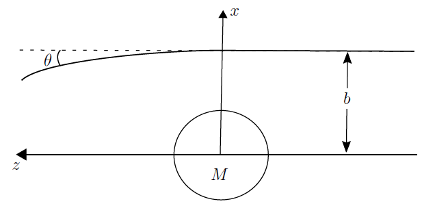
Figure 1: Path of a light ray in the gravitational field of a static spherically symmetric body of mass $M$.

The deflection angle for a light ray passing by a static spherically symmetric mass distribution is therefore [22]

$$\theta=\left|\frac{\Delta k_{x}}{k_{z}}\right|=\frac{1}{c^{2}}\int^{\infty}_{-\infty}\frac{\partial}{\partial x}\left(V+W\right)\Big{|}_{x=b}\,dz.$$ (43)

Inserting (22) and (25) into (43), we obtain the MCG deflection angle

$$\theta_{\textrm{MCG}}=\theta_{\textrm{GR}}-\frac{3GMb}{2c^{2}}\int^{\infty}_{-\infty}\left[\frac{1+\frac{mc}{\hbar}\sqrt{b^{2}+z^{2}}}{(b^{2}+z^{2})^{3/2}}\,e^{-\frac{mc}{\hbar}\sqrt{b^{2}+z^{2}}}\right]dz,$$ (44)

where

$$\theta_{\textrm{GR}}=\frac{2GMb}{c^{2}}\int^{\infty}_{-\infty}\left[\frac{1}{(b^{2}+z^{2})^{3/2}}\right]dz$$ (45)

is the general relativistic deflection angle. Integrating (44) numerically, with $M=M_{\odot}=1.9891\times 10^{30}\,\mbox{kg}$ and $b=6.955\times 10^{8}\,\mbox{m}$, we can find the evaluation of the solar MCG deflection angle for different values of $m$. The result depicted in Fig. 2 shows that we must have $m\gtrsim 3.5\times 10^{-51}\,\mbox{kg}$ in order to the solar MCG deflection angle agrees with the measured solar GR deflection angle $\theta_{\textrm{GR}}\sim 1.75^{\prime\prime}$ [23].

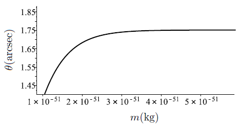
Figure 2: Deflection angle as a function of mass for light rays grazing the Sun in MCG.

5 Radar echo delay

Let us consider a light signal that moves along a straight line (parallel to the $z$-axis) connecting two points $z_{1}$ and $z_{2}$ in the gravitational field of a static spherically symmetric massive body (see Fig. 3). It follows from (16) and (40) that the change in $k_{z}$ along the straight line is given by

$$dk_{z}=-\frac{\omega}{c^{3}}\frac{\partial}{\partial z}\left(V+W\right)dz.$$ (46)

Substituting (22) and (25) into (46), and integrating, we find

$$k_{z}(z)-\frac{\omega}{c} = -\,\frac{2GM\omega}{c^{3}}\int^{z}_{\infty}\Bigg{[}\frac{z^{\prime}}{(b^{2}+z^{\prime 2})^{3/2}}-\frac{3}{4}\frac{z^{\prime}e^{-\frac{mc}{\hbar}\sqrt{b^{2}+z^{\prime 2}}}}{(b^{2}+z^{\prime 2})^{3/2}}$$ (47)

$$-\,\frac{3}{4}\frac{\frac{mc}{\hbar}z^{\prime}e^{-\frac{mc}{\hbar}\sqrt{b^{2}+z^{\prime 2}}}}{\sqrt{b^{2}+z^{\prime 2}}}\Bigg{]}dz^{\prime},$$

where we used $k_{z}(\infty)=\omega/c$.

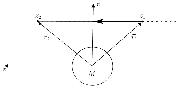
Figure 3: Path of a light signal between two points in the gravitational field of a static spherically symmetric mass distribution.

The insertion of (47) into the delay in the time it takes the light signal to travel from $z_{1}$ to $z_{2}$ and back [22]

$$\Delta t=\frac{2}{\omega}\int_{z_{1}}^{z_{2}}\left[k_{z}(z)-\frac{\omega}{c}\right]\,dz$$ (48)

gives

$$\Delta t_{\textrm{MCG}}=\Delta t_{\textrm{GR}}+\frac{3GM}{c^{3}}\int_{z_{1}}^{z_{2}}\left[\int^{z}_{\infty}\left(\frac{1+\frac{mc}{\hbar}\sqrt{b^{2}+z^{\prime 2}}}{(b^{2}+z^{\prime 2})^{3/2}}\,z^{\prime}e^{-\frac{mc}{\hbar}\sqrt{b^{2}+z^{\prime 2}}}\right)dz^{\prime}\right]dz,$$ (49)

where

$$\Delta t_{\textrm{GR}}=-\frac{4GM}{c^{3}}\int_{z_{1}}^{z_{2}}\left[\int^{z}_{\infty}\left(\frac{z^{\prime}}{(b^{2}+z^{\prime 2})^{3/2}}\right)dz^{\prime}\right]dz$$ (50)

is the general relativistic time delay. For a light signal traveling between the Earth (at $z_{1}<0$) and Mercury (at $z_{2}>0$) on opposite sides of the Sun, we must set $M=M_{\odot}$, $b=6.955\times 10^{8}\,\mbox{m}$, $z_{1}=-\,14.9\times 10^{10}\,\mbox{m}$ and $z_{2}=5.8\times 10^{10}\,\mbox{m}$. Using these values, a numerical integration of (49) gives the result shown in Fig. 4, which leads to the conclusion that the MCG time delay is consistent with the observed general relativistic value $\Delta t_{\textrm{GR}}\sim 220\,\mu\mbox{s}$ [24] for $m\gtrsim 2\times 10^{-51}\,\mbox{kg}$.

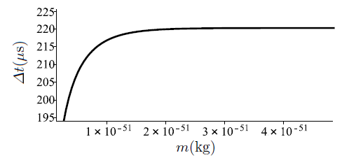
Figure 4: Time delay as a function of mass for light traveling between the Earth and Mercury in MCG.

6 Perihelion precession of Mercury

Now we consider the motion of a test particle of mass $m^{\prime}$ in orbit around a static spherically symmetric body of mass $M$ (see Fig. 5). Using polar coordinates $r$ and $\phi$ in the orbital plane ($\theta=\pi/2$), we can write the total Newtonian energy of the system as

$$E=\frac{1}{2}\mu(\dot{r}^{2}+r^{2}\dot{\phi}^{2})+U(r),$$ (51)

where $\mu=m^{\prime}M/(m^{\prime}+M)$ is the reduced mass and a dot denotes $d/dt$.

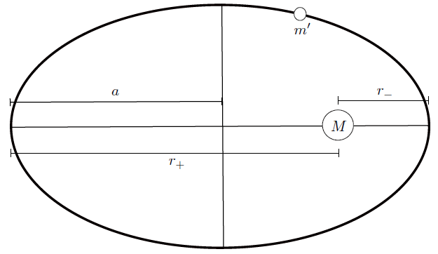
Figure 5: Test particle orbiting a static spherically symmetric mass distribution.

Considering the conservation of the angular momentum

$$J=\mu r^{2}\dot{\phi}=\mbox{constant},$$ (52)

we rewrite (51) in the form

$$E=\frac{1}{2}\mu\dot{r}^{2}+\frac{J^{2}}{2\mu r^{2}}+U(r),$$ (53)

which gives

$$\dot{r}=\frac{dr}{dt}=\sqrt{\frac{2}{\mu}\left[E-U(r)\right]-\frac{J^{2}}{\mu^{2}r^{2}}}.$$ (54)

By writing (52) as $d\phi=Jdt/\mu r^{2}$, substituting $dt$ from (54) and integrating, we obtain

$$\phi=\int{\frac{Jdr/r^{2}}{\sqrt{2\mu\left[E-U(r)\right]-J^{2}/r^{2}}}}+\mbox{constant}.$$ (55)

According to (55), during the time in which $r$ varies from $r_{+}$ to $r_{-}$ and back, the radius vector turns through an angle

$$\Delta\phi=2\int_{r_{-}}^{r_{+}}{\frac{Jdr/r^{2}}{\sqrt{2\mu\left[E-U(r)\right]-J^{2}/r^{2}}}}.$$ (56)

Substituting a potential energy of the type

$$U(r)=-\frac{GM\mu}{r}+\delta U(r),$$ (57)

where $\delta U$ is a small correction to the Newtonian potential energy, into (56) and expanding the integrand in powers of $\delta U$, we find that the zero-order term in the expansion gives $2\pi$, and the first-order term gives the precession of the orbit per revolution [25]

$$\delta\phi=-\frac{2p}{GM\mu e}\int_{0}^{\pi}{r^{2}\frac{d}{dr}\left[\delta U(r)\right]\cos{\phi}\,d\phi},$$ (58)

where

$$r=\frac{p}{(1+e\cos{\phi})},$$ (59)

with $p=a(1-e^{2})$ being the semilatus rectum, $a$ the semi-major axis and $e$ the eccentricity of the orbital ellipse. In terms of the variable $z=\cos{\phi}$, we can write (58) in the more useful form [26]

$$\delta\phi=-\frac{2p}{GM\mu e^{2}}\int_{-1}^{1}{\frac{z}{\sqrt{1-z^{2}}}\frac{d}{dz}\left[\delta U(z)\right]\,dz}.$$ (60)

In order to find the MCG potential energy, we substitute (16) into the normalization of the four-velocity

$$g_{\mu\nu}u^{\mu}u^{\nu}=-c^{2},$$ (61)

which, in polar coordinates in the orbital plane, gives

$$-\left(1+\frac{2V}{c^{2}}\right)c^{2}t^{\prime 2}+\left(1-\frac{2W}{c^{2}}\right)\left(r^{\prime 2}+r^{4}\phi^{\prime 2}\right)=-c^{2},$$ (62)

where a prime denotes $d/d\tau$. Considering that the Lagrangian of the system is given by

$$\mathcal{L}=\frac{1}{2}\mu g_{\mu\nu}u^{\mu}u^{\nu}=\frac{1}{2}\mu\left[-\left(1+\frac{2V}{c^{2}}\right)c^{2}t^{\prime 2}+\left(1-\frac{2W}{c^{2}}\right)\left(r^{\prime 2}+r^{4}\phi^{\prime 2}\right)\right],$$ (63)

we find the total energy

$$E_{\mathrm{tot}}=-\frac{\partial\mathcal{L}}{\partial t^{\prime}}=\mu\left(1+\frac{2V}{c^{2}}\right)c^{2}t^{\prime}$$ (64)

and the angular momentum

$$J=\frac{\partial\mathcal{L}}{\partial\phi^{\prime}}=\mu\left(1-\frac{2W}{c^{2}}\right)r^{4}\phi^{\prime}.$$ (65)

The substitution of $t^{\prime}$ and $\phi^{\prime}$ from (64) and (65) into (62) gives

$$-\left(1+\frac{2V}{c^{2}}\right)^{-1}\frac{E_{\mathrm{tot}}^{2}}{\mu^{2}c^{2}}+\left(1-\frac{2W}{c^{2}}\right)r^{\prime 2}+\left(1-\frac{2W}{c^{2}}\right)^{-1}\frac{J^{2}}{\mu^{2}r^{2}}=-c^{2},$$ (66)

which can be rewriting in the form

$$\frac{E_{\mathrm{tot}}^{2}}{c^{2}}=\left(1+\frac{2V}{c^{2}}\right)\mu^{2}\left[\left(1-\frac{2W}{c^{2}}\right)r^{\prime 2}+\left(1-\frac{2W}{c^{2}}\right)^{-1}\frac{J^{2}}{\mu^{2}r^{2}}+c^{2}\right].$$ (67)

By inserting (22) and (25) into (67), keeping only the first-order kinetic term and the potential terms up to second order in $1/r$, taking the Newtonian limit $d/d\tau\rightarrow d/dt$, and making some algebra, we obtain

$$E=\frac{1}{2}\mu\dot{r}^{2}+\frac{J^{2}}{2\mu r^{2}}-\frac{GM\mu}{r}+\frac{GM\mu}{r}e^{-\frac{mc}{\hbar}r}-\frac{GMJ^{2}}{\mu c^{2}r^{3}}(1-e^{-\frac{mc}{\hbar}r}),$$ (68)

where

$$E=\frac{E_{\mathrm{tot}}^{2}-\mu^{2}c^{4}}{2\mu c^{2}}$$ (69)

is the usual Newtonian energy.

Comparing (68) with (53) and (57), we can see that

$$\delta U(r)=\frac{GM\mu}{r}e^{-\frac{mc}{\hbar}r}-\frac{GMJ^{2}}{\mu c^{2}r^{3}}(1-e^{-\frac{mc}{\hbar}r})$$ (70)

for MCG. Finally, using $r=p/(1+ez)$ and $J^{2}=GM\mu^{2}p$ in (70), and substituting into (60), we arrive at the MCG precession per revolution

$$\delta\phi_{\textrm{MCG}} = \delta\phi_{\textrm{GR}}-\frac{2p}{e}\int_{-1}^{1}\frac{z}{\sqrt{1-z^{2}}}\Bigg{[}\frac{1}{p}+\frac{mc}{\hbar(1+ez)}+\frac{3GM(1+ez)^{2}}{c^{2}p^{2}}$$ (71)

$$+\,\frac{GMm(1+ez)}{\hbar cp}\Bigg{]}\mbox{exp}\left(-\frac{mc}{\hbar}\frac{p}{1+ez}\right)dz,$$

where

$$\delta\phi_{\textrm{GR}}=\frac{6GM}{ec^{2}p}\int_{-1}^{1}{\frac{z}{\sqrt{1-z^{2}}}\left(1+ez\right)^{2}\,dz}=\frac{6\pi GM}{c^{2}p}$$ (72)

is the general relativistic precession per revolution.

Using $M=M_{\odot}$, $e=0.2056$ and $p=6.686\times 10^{7}\,\mbox{km}$ in (71), and integrating numerically, we find the MCG precession per century for the orbit of Mercury around the Sun, which is shown in Fig. 6. Assuming that the measured precession for Mercury is $\sim 43^{\prime\prime}$ per century [27], it follows that we must have $m\gtrsim 2.5\times 10^{-52}\,\mbox{kg}$.

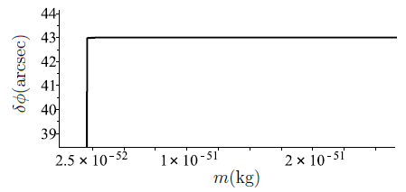
Figure 6: Precession per century for the orbit of Mercury around the Sun as a function of mass in MCG.

7 Final remarks

In the present paper, we have compared the predictions of MCG with some solar system observations, namely, the deflection of light by the Sun, the radar echo delay and the perihelion precession of Mercury. In particular, it was shown that the linear MCG predictions are consistent with these three solar system phenomena provided we have $m\gtrsim 3.5\times 10^{-51}\,\mbox{kg}$. Despite this lower bound on the graviton mass is in agreement with the bound $m\gtrsim 10^{-38}\,\mbox{kg}$ imposed by Cavendish like experiments [28] and the measured decrease of the orbital period of binary systems [12], it makes the theory unable to explain galaxy rotation curves and the deflection of light by galaxies without dark matter. However, the conformal symmetry of the theory allows us to introduce an extra scalar field with zero vacuum expectation value in the matter part of the theory [29]. Although more studies on this are needed, this extra scalar may be a good candidate for dark matter.

With the results obtained here, we have taken another important step towards confirming MCG as a serious candidate to solve the GR problems. Clearly, there are still many steps to be taken such as whether the theory is consistent with the early universe data or whether it solves the dark matter and singularity problems, among others. We will continue to work in the hope of overcoming some of these steps in the near future.

References

• [1] H. Weyl, Sitz. Berichte d. Preuss. Akad. d. Wissenschaften, 465 (1918).
• [2] T. Kaluza, Sitzungsber. Preuss. Akad. Wiss. Berlin., 966 (1921).
• [3] C. Brans and R. H. Dicke, Phys. Rev. 124, 925 (1961).
• [4] P. G. Bergmann, Int. J. Theo. Phys. 1, 25 (1968).
• [5] M. Milgrom, Astrophys. J. 270, 365 (1983).
• [6] P. Hořava, Phys. Rev. D 79, 084008 (2009).
• [7] P. D. Mannheim and J. G. O’Brien, Phys. Rev. D 85, 124020 (2012).
• [8] P. D. Mannheim, Phys. Rev. D 75, 124006 (2007).
• [9] G. ’t Hooft, Found. Phys. 41, 1829 (2011).
• [10] F. F. Faria, Adv. High Energy Phys. 2014, 520259 (2014).
• [11] F. F. Faria, Adv. High Energy Phys. 2019, 7013012 (2019).
• [12] F. F. Faria, Eur. Phys. J. C 80, 645 (2020).
• [13] F. F. Faria, Eur. Phys. J. C 76, 188 (2016).
• [14] F. F. Faria, Eur. Phys. J. C 77, 11 (2017).
• [15] F. F. Faria, Eur. Phys. J. C 78, 277 (2018).
• [16] F. F. Faria, Mod. Phys. Lett. A. 36, 2150115 (2021).
• [17] N. Matsuo, Gen. Relativ. Gravit. 22, 561 (1990).
• [18] B. L. Giacchini, Phys. Lett. B 766, 306 (2017).
• [19] E. E. Flanagan, Phys. Rev. D 74, 023002 (2006).
• [20] P. D. Mannheim, Prog. Part. Nucl. Phys. 56, 340 (2006).
• [21] P. I. Dyadina, S. P. Labazova and S. O. Alexeyev, JETP 156, 905 (2019).
• [22] H. C. Ohanian and R. Ruffini, Gravitation and Spacetime (Cambridge University Press, New York, 2013).
• [23] D. G. Bruns, Class. Quant. Grav. 35, 075009 (2018).
• [24] B. Bertotti, L. Iess and P. Tortora, Nature 425, 374 (2003).
• [25] L. D. Landau and E. M. Lifshitz, Mechanics (Butterworth-Heinemann, Oxford, 1976).
• [26] G. S. Adkins and J. McDonnell, Phys. Rev. D 75, 082001 (2007).
• [27] R. S. Park et al., Astron. J. 153, 121 (2017).
• [28] E. Adelberger et al., Prog. Part. Nucl. Phys. 62, 102 (2009).
• [29] F. F. Faria, arXiv:1903.04893 [hep-th].