Three-dimensional non-equilibrium Potts systems with magnetic friction

Abstract

We study the non-equilibrium steady states that emerge when two interacting three-dimensional Potts blocks slide on each other. As at equilibrium the Potts model exhibits different types of phase transitions for different numbers $q$ of spin states, we consider the following three cases: $q=2$ (i.e. the Ising case), $q=3$, and $q=9$, which at equilibrium yield respectively a second order phase transition, a weak first order transition and a strong first order transition. In our study we focus on the anisotropic character of the steady states that result from the relative motion and discuss the change in finite-size signatures when changing the number $q$ of spin states.

I Introduction

Much of our knowledge on non-equilibrium steady states results from in-depth studies of transport models Cho11 , of driven systems Sch95 , as well as of reaction-diffusion systems Odo08 . Our current understanding of non-equilibrium phase transitions has also profited greatly from the investigation of model systems Hen08 ; Tau14 . Similar to the situation at equilibrium, non-equilibrium phase transitions can either be continuous or discontinuous. Furthermore, cases of strongly anisotropic phase transitions are also encountered far from equilibrium (see, e.g., the driven lattice gas Sch95 ; Kat83 ).

Spin models with magnetic friction and the related sheared spin models provide interesting classes of non-equilibrium systems that possess many intriguing properties Kad08 ; Fus08 ; Mag09 ; Mag09a ; Huc09 ; Hil11 ; Igl11 ; Mag11 ; Mag11a ; Ang12 ; Huc12 ; Mag13 . The term magnetic friction is used to characterize the situation where spin correlations between moving magnetic systems lead to energy dissipation. As a result the system settles into a non-equilibrium steady state. Examples include a magnetic tip moving on a magnetic surface described as a classical Heisenberg system Fus08 ; Mag09 ; Mag09a ; Mag11 ; Mag11a ; Mag13 as well as bulk spin systems moving relative to each other Kad08 ; Hil11 ; Igl11 ; Ang12 ; Huc12 . In Kad08 Kadau et al studied two coupled two-dimensional semi-infinite Ising models that slide on each other. This sliding motion stabilizes the spin structure at the boundary, yielding an enhancement of the local magnetization in cases where equal coupling strengths are considered everywhere in the system. Consequently, the boundary layers undergo a local phase transition at a temperature above the equilibrium bulk critical temperature. This boundary phase transition temperature can be computed exactly for the two-dimensional Ising model in the limiting case of infinite relative speed Huc09 . In Igl11 two-dimensional systems with magnetic friction composed of Potts spins with $q$ states (the case $q=2$ being the Ising case) were considered. This study revealed the existence of exotic non-equilibrium boundary phase transitions for large number of spin states $q$, i.e. in situations where the equilibrium bulk system undergoes a discontinuous transition. Indeed, depending on the strength of the boundary couplings between the two sub-systems moving relatively to each other a change of the character of the non-equilibrium boundary phase transition is observed, being continuous for weak boundary couplings and discontinuous when these couplings are strong. Hucht introduced in Huc09 other Ising models with moving boundaries, including three-dimensional geometries as well as sheared Ising systems. Later studies of some of these Ising systems Ang12 ; Huc12 focused on the strongly anisotropic character of the non-equilibrium phase transitions encountered in these systems.

In the following we extend this line of research to coupled three-dimensional Potts blocks that slide on each other. In three-dimensional bulk systems the Potts model displays different types of equilibrium phase transitions as a function of the number of states $q$. We study in the following the cases $q=2$ with a continuous equilibrium bulk phase transition, $q=3$ with a weak discontinuous phase transition in the bulk system, and $q=9$ where the bulk transition is strongly discontinuous. Our aim is to develop a qualitative understanding of the non-equilibrium steady states induced by the sliding of the blocks and to understand how the properties of the non-equilibrium boundary phase transitions vary when changing the strength of the coupling between the blocks or the speed of the relative motion.

Our paper is organized in the following way. In the next Section we provide a more detailed discussion of the studied geometry as well as of the local (boundary and line) quantities used to elucidate the properties of our non-equilibrium systems. Section III is devoted to the numerical investigation of systems composed of two Potts blocks that are in relative motion with respect to each other. Using local (boundary and line) quantities we investigate the magnetic properties of these driven systems as a function of relative speed as well as of the strength of the coupling between the two sub-systems. We discuss the finite-size signatures in these anisotropic systems and elucidate how they change with the number $q$ of spin states. We conclude in Section IV.

II Models

We consider in this work three-dimensional models composed of two $q$-state Potts systems that are coupled at their surfaces and that move along their boundaries with a constant relative speed $v$. Each of the systems is characterized by a lattice and a Hamiltonian of the form

$${\mathcal{H}}=-J\sum\limits_{\langle\bf{r},\bf{r}^{\prime}\rangle}\,\delta\left(S_{\bf{r}}-S_{\bf{r}^{\prime}}\right)$$ (1)

where the sum is over nearest neighbor lattice sites. The coupling constant $J$ is chosen to be positive. $\delta$ is the Kronecker delta, with $\delta(x)=1$ if $x=0$ and zero otherwise. At every lattice site ${\bf r}$ we have a Potts spin $S_{\bf{r}}$ that takes on the values $S_{\bf{r}}=0,1,\cdots,q-1$.

A Potts system with $q=2$ corresponds to the Ising model and exhibits in the thermodynamic limit a second order phase transition between a disordered high temperature phase and an ordered low temperature phase. In a three-dimensional bulk system this transition becomes a first order transition for $q\geq 3$. In our study we focus on three $q$ values, $q=2$, 3, and 9, corresponding to a second order transition, a weak first order transition and a strong first order transition, respectively.

Assuming that the surfaces are perpendicular to the $z$-direction and that the relative motion is in the $y$-direction, we couple the two Potts systems through the time-dependent interaction term

$${\mathcal{V}}(t)=-J_{b}\sum\limits_{x_{1},y_{1}}\,\delta\left(S_{{\bf r}_{1}}-S_{{\bf r}_{2}(t)}\right)~{},$$ (2)

where ${\bf r}_{1}=(x_{1},y_{1},z_{1})$ is a lattice point in the surface layer $z_{1}$ of system 1, whereas ${\bf r}_{2}(t)=(x_{2},y_{2},z_{2})=(x_{1},y_{1}+vt,z_{1}+1)$ is a surface point of system 2 located above the site ${\bf r}_{1}$ but shifted in $y$-direction by the amount $vt$. This interaction term gives rise to magnetic friction and entails that the system settles into a non-equilibrium steady state. Besides varying the dimensions of the sub-systems and the relative speed $v$, we will also consider different coupling strength ratios $\kappa=J_{b}/J$ where $J_{b}$ is the strength of the couplings between the sub-systems, whereas $J$ is the strength of the couplings within the sub-systems.

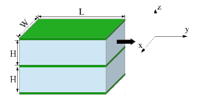
Figure 1: (Color online) Schematic picture of two identical sub-systems with relative motion in the $y$-direction. The two sub-systems are blocks composed of $W\times L\times H$ spins, with periodic boundary conditions in all three directions. Boundaries between the two sub-systems are indicated by the green (dark) areas.

The geometry discussed in this paper is shown in Fig. 1. Our system is composed of two identical blocks where the upper block moves relative to the lower one. Typically the width $W$ and height $H$ vary between 20 and 80 lattice sites. We investigate systems with length $L$ up to 240 sites in order to check for anisotropy effects resulting from the relative motion in $y$-direction. As we are interested in the boundary properties, we use periodic boundary conditions in all three directions so that every block experiences magnetic friction at two separate boundaries.

In order to elucidate the properties close to the boundary separating the two sub-systems we focus on local quantities. Examples include the steady-state magnetization density in layer $z$ at temperature $T$

$$m(z,T)=\left(\frac{q\langle N_{m}(z,T)\rangle}{N(z)}-1\right)/\left(q-1\right)$$ (3)

and the corresponding fluctuations around the mean layer magnetization density

$$\chi(z,T)=\frac{1}{k_{B}TN(z)}\left[\langle N_{m}(z,T)^{2}\rangle-\langle N_{m}(z,T)\rangle^{2}\right]~{}.$$ (4)

Here, $\langle N_{m}(z,T)\rangle$ is the average number of majority spins in layer $z$ at temperature $T$: $\langle N_{m}(z,T)\rangle=\mbox{max}(\langle N_{0}(z,T)\rangle,\cdots,\langle N_{q-1}(z,T)\rangle)$, where $\langle N_{k}(z,T)\rangle$ is the average number of spins in state $k$ in layer $z$. The total number of spins in layer $z$ is denoted by $N(z)$, with $N(z)=W\times L$ for the rectangular layers in the sub-systems shown in Fig. 1. Another quantity of interest is the energy density in each layer $E(z,T)$ and the corresponding specific heat $C(z,T)=dE(z,T)/dT$. The boundary quantities are obtained by averaging over all equivalent boundary layers. For the two-block system of Fig. 1 we have four equivalent boundary layers, located at $z=1$, $H$, $H+1$, and $2H$, over which we can average in order to determine, for example, the mean boundary magnetization density $m_{b}$ or the mean boundary specific heat $C_{b}$.

In order to probe for possible anisotropy effects resulting from the relative motion of the coupled sub-systems, we also consider in the boundary layers the average line magnetizations in $x$- and $y$-directions, defined as

$$m_{x}(y_{0},T) = \left(\frac{q\langle N^{x}_{m}(y_{0},T)\rangle}{N_{x}}-1\right)/\left(q-1\right)$$ (5)

$$m_{y}(x_{0},T) = \left(\frac{q\langle N^{y}_{m}(x_{0},T)\rangle}{N_{y}}-1\right)/\left(q-1\right)$$ (6)

where $\langle N^{x}_{m}(y_{0},T)\rangle$ (respectively $\langle N^{y}_{m}(x_{0},T)\rangle$) is the average number of majority spins in column $y_{0}$ (respectively row $x_{0}$) in the boundary layer at temperature $T$, whereas $N_{x}$ (respectively $N_{y}$) is the total number of spins in each column (respectively row). For the rectangular layers of the sub-systems in Fig. 1 we have that $N_{x}=W$ and $N_{y}=L$. As our systems are translationally invariant in $x$- and $y$-directions, the choice of column $y_{0}$ and row $x_{0}$ is not important.

These magnetic properties are computed in Monte Carlo simulations where we follow previous work and implement the relative motion between the two sub-systems by combining single spin updates and shifts of a sub-system as a whole. For the single spin updates we use the standard heat-bath algorithm. In order to simulate a system where one sub-system slides with speed $v$ with respect to the other, we shift this sub-system by one lattice constant after $N/v$ random single spin updates, where $N$ is the total number of spins in the system. One time step therefore consists of $N$ proposed single spin updates and $v$ translations. Note that in the implementation we do not shift the sub-system that slides, but instead only rewire the couplings at the boundary, as this involves much fewer computational operations.

III Sliding Potts blocks

In this Section we study the magnetic properties of three-dimensional Potts spin blocks sliding past each other. Results for these systems are scarce, and the only previous result that directly relates to our study is the calculation of the shift of the critical temperature for the case of two Ising blocks with couplings of only one strength (i.e. $J_{b}=J=1$) moving with infinite relative speed. Indeed, in that case the critical temperature of the non-equilibrium system can be expressed as a function of the zero-field equilibrium susceptibility Huc09 . From the eighth-order high temperature series for the equilibrium susceptibility one finds in Potts units the critical temperature $T_{c}=2.40(5)$ Huc09 , substantially larger than the critical temperature $T_{c}=2.256$ of the three-dimensional equilibrium Ising model.

On general grounds, the phase transition in our system is expected to be strongly anisotropic, similar to what is observed in related cases Ang12 ; Huc12 . In what follows, we indeed discuss the anisotropic properties close to the phase transition, and this in cases where the bulk transition is either continuous or discontinuous. We limit ourselves to a qualitative discussion, leaving a more quantitative study (which requires for the cases of large number of states $q$ resources not currently available to us) for a later time.

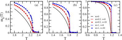
Figure 2: (Color online) Boundary magnetization density as a function of temperature $T$ for two Potts blocks that are either both at rest ($v=0$) or where one of the blocks is moving with respect to the other with speed $v=10$. Data for different small values of the coupling strength ratio $\kappa$ are shown. For $\kappa=0$ the two blocks are uncoupled, whereas for $\kappa=1$ the couplings at the boundary have the same strength as the couplings inside the bulk. The number of states are (a) $q=2$, (b) $q=3$, and (c) $q=9$. Every block is composed of $80\times 80\times 80$ spins. The data result from averaging over at least ten independent runs, and error bars are smaller than the symbol sizes.

Fig. 2 shows for systems composed of blocks with $80\times 80\times 80$ spins the temperature-dependent boundary magnetization density $m_{b}(T)$ for a variety of cases with vanishing or small coupling strength ratios $\kappa$. The full lines correspond to equilibrium situations, whereas the symbols give values in non-equilibrium steady states. For $\kappa=0$ (black lines) the two sub-systems are uncoupled, and $m_{b}$ is then the surface magnetization of an equilibrium system with open boundary conditions. For all values of $q$ the surface magnetization vanishes continuously with increasing temperature, and this even so for $q\geq 3$ the equilibrium bulk transition is discontinuous. This surface-induced disordering effect is well known for systems with free surfaces where the bulk undergoes a discontinuous transition Lip82 ; Lip83 ; Sch96 ; Igl99 ; Haa00 ; Li13 . For $\kappa=1$ and $v=0$ we recover the bulk equilibrium system with a discontinuous phase transition for $q\geq 3$, i.e. there is a critical value of $\kappa$ between 0 and 1 at which the character of the equilibrium boundary transition changes, see Fig. 2.

Only minor differences between the equilibrium and non-equilibrium cases with $v=10$ can be seen in Fig. 2 for $0<\kappa\leq 1$. A closer look reveals for $q=2$ and $\kappa=1$ that the symbols lie systematically above the equilibrium results, in agreement with the predicted shift of the critical temperature Huc09 . The same holds true for $q=3$, whereas for $q=9$ equilibrium and non-equilibrium data are identical within error bars. For the Ising case the data are compatible with the expected shift of $T_{c}$ Huc09 , but seem to indicate a much smaller increase than that obtained by Hucht for the case $v=\infty$ from (admittedly rather short) high temperature series for the equilibrium susceptibility. The reader, however, should note that a square boundary layer is not the most appropriate geometry close to the phase transition. As we argue below, anisotropic samples are much better suited in order to obtain quantitatively correct data in vicinity of the strongly anisotropic phase transition.

In a previous study of the two-dimensional Potts system with $q=9$ states where two halves of the system slide on top of each other Igl11 a change of the character of the boundary transition as a function of $\kappa$ was also observed: for small values of $\kappa$ the boundary phase transition is continuous and takes place at the bulk transition temperature, whereas for large values of $\kappa$ the transition is discontinuous and the transition temperature is shifted to values larger than the bulk transition temperature. However, in this case the ordering of the boundary (which is a one-dimensional object) at a temperature above the bulk transition temperature is a purely non-equilibrium effect as in equilibrium a one-dimensional spin system with short-range interactions does not support long-range order.

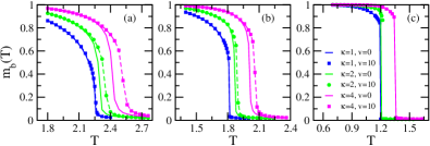
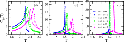
Figure 3: (Color online) (a)-(c) Boundary magnetization density $m_{b}$ and (d)-(f) boundary specific heat $C_{b}$ as a function of temperature $T$ for two Potts blocks that are either both at rest ($v=0$) or where one of the blocks is moving with respect to the other with speed $v=10$. Data for different large values of the coupling strength ratio $\kappa$ are shown. The number of states are (a,d) $q=2$, (b,e) $q=3$, and (c,f) $q=9$. The relative motion stabilizes the ordering of the boundary which results in an additional shift of the local transition temperature. This is clearly visible in the data for $q=2$ and $q=3$. Every block is composed of $80\times 80\times 80$ spins. The data result from averaging over at least ten independent runs, and error bars are smaller than the symbol sizes.

When further increasing the strength of the coupling between the sub-systems, the trends already visible in Fig. 2 persist and become very pronounced. This is illustrated in Fig. 3 through the temperature dependence of the boundary magnetization density $m_{b}(T)$ as well as of the boundary specific heat $C_{b}(T)$. We note that for all values of $q$ and $\kappa>1$ the phase transition temperature is larger than that of the perfect equilibrium bulk system with $v=0$ and $\kappa=1$. This shift is readily understood for the equilibrium case (full lines) as the boundary region with a strong coupling between the sub-systems behaves like a two-dimensional object that orders at a higher temperature than the bulk. The sliding motion further enhances this tendency for increased ordering, and for $q=2$ and $q=3$ an additional increase of the boundary transition temperature, that results from the motion, is observed (see the symbols and dashed lines in Fig. 3). For very large values of $q$, see the case $q=9$ in Fig. 3c and 3f, the relative motion only results in very minor changes with respect to the equilibrium situation.

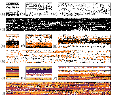
Figure 4: (Color online) Snapshots of one of the boundaries of a system formed by two blocks with $20\times L\times 10$ spins. The speed is $v=10$ and the ratio of coupling strengths is $\kappa=9$. (a)-(d) $q=2$ and $T=3$, (e)-(h) $q=3$ and $T=2.45$, (i)-(l) $q=9$ and $T=1.55$. The length of the sample is (a) $L=20$, (b) $L=40$, (c) $L=80$, and (d) $L=160$, and similarly for the other two values of $q$. The different colors correspond to the different states of the spins.

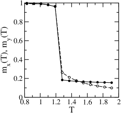
Figure 5: Line magnetization densities in $x$ (filled squares) and $y$ (open circles) directions for a system with $q=9$, $\kappa=9$, and $v=10$ composed of blocks containing $20\times 160\times 10$ spins. A typical spin configuration for that system at $T=1.55$ is shown in Fig. 4(l).

Looking at boundary quantities like those in Fig. 2 and 3 does not provide a comprehensive view of our systems, as they do not reveal the anisotropy effects induced by the relative motion of the blocks. Fig. 4 shows some typical spin configurations in the boundary layer for systems with large boundary couplings and different aspect ratios, taken at temperatures close to the boundary phase transition. We focus in the following on the $q=9$ states case shown in Fig. 4(i)$-$(l), but the same effects are observed for other number of spin states, see the figure. Starting with a square boundary in panel (i), we double from panel to panel the length of the boundary in direction of the relative motion until the aspect ratio is 8 for panel (l). The motion of the blocks induces additional correlations in the sliding direction, and one therefore expects anisotropy effects to show up as direction-dependent correlation lengths and, in the ordered phase, anisotropically shaped ordered domains. For the example shown in panel (i) to (l), the anisotropy effects in systems with small aspect ratios take the form of almost completely ordered lines in the direction of motion (horizontal or $y$-direction), whereas in the direction perpendicular to the motion (vertical or $x$-direction) the spins are much more disordered. Even so we are close to the phase transition, the smallness of the horizontal dimension yields as an artifact a very large line magnetization. Increasing the length of the system in that direction allows to capture better and better the fluctuations and yields for the largest length shown in panel (l) configurations with a comparable level of order in both directions. This is illustrated in Fig. 5 where we compare the line magnetization densities in the different directions for the system with blocks containing $20\times 160\times 10$ spins.

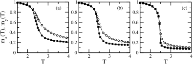
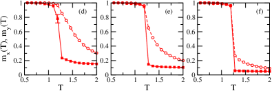
Figure 6: (Color online) Line magnetization densities in $x$ (filled squares) and $y$ (open circles) directions for $\kappa=9$. (a)-(c) $q=2$ and (d)-(f) $q=9$. The sizes of the blocks, which move with relative speed $v=10$, are $L\times L\times 20$, with (a,d) $L=20$, (b,e) $L=40$, and (c,f) $L=160$. The data result from averaging over at least 10 independent runs. Error bars are only shown when the error is larger than the symbol size.

Fig. 6 shows some quantitative data for the line magnetization densities $m_{x}$ and $m_{y}$ (see equations (5) and (6)) for $q=2$ and $q=9$, with $\kappa=9$. In order to compare finite-size effects, we consider square boundaries with $L\times L$ spins, $L$ ranging from 20 to 160. The data for $q=2$ in the first row show the expected finite-size behavior of the line magnetization close to an anisotropic critical point: in the direction of motion fluctuations are more strongly constrained, which yields a higher level of ordering as witnessed by the larger line magnetization density $m_{y}$ (open symbols). Increasing the system size allows to capture better and better the fluctuations, and the two densities get increasingly comparable. An interesting additional effect shows up when considering the system with a discontinuous bulk transition as it is the case for $q=9$, see second row of Fig. 6. As seen in Fig. 3c, the boundary transition is also discontinuous in that case for large values of $\kappa$, as evidenced by the discontinuity in the boundary magnetization. However, for the smaller systems only the line magnetization $m_{x}$ in direction perpendicular to the motion (filled squares) displays a discontinuous character. The line magnetization $m_{y}$ in direction of the motion shows a smooth behavior, see panel (d), reminiscent of that observed in panel (a) for $q=2$ where the boundary transition is continuous. It is only for larger systems that also $m_{y}$ starts to reveal a large jump indicating the discontinuous character of the transition in the thermodynamic limit.

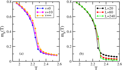
Figure 7: (Color online) Boundary magnetization densities for the Ising model as a function of temperature. (a) Shift of the boundary magnetization density as a function of the speed $v$ in systems composed of blocks containing $20\times 20\times 20$ spins. (b) Boundary magnetization densities for anisotropically shaped samples with $40\times L\times 20$ spins in each block that move with relative speed $v=\infty$. Based on all our data, we estimate the critical temperature to be $T_{c}=2.34(2)$.

As discussed previously, the data shown in Fig. 2 for $\kappa=1$ seem to indicate for the Ising case a rather small shift of the critical temperature compared to the equilibrium case. We have another look at this in Fig. 7 where we consider samples moving with different speeds as well as different anisotropic shapes. We here consider also the case $v=\infty$ where for the update of a boundary spin, located at, say, the top of the lower block at site ${\bf r}_{1}=(x_{1},y_{1},H)$, we connect this spin via the coupling term (2) to a randomly selected spin with the same $x$-coordinate but located in the neighboring boundary layer Huc09 , i.e. this second spin has the coordinates ${\bf r}_{2}=(x_{1},y_{2},H+1)$ with $1\leq y_{2}\leq L$. Fig. 7a illustrates the shift of the magnetization densities due to the relative motion for blocks composed of $20\times 20\times 20$ spins. As shown in Fig. 7b, strong finite-size effects do not allow to obtain reliable estimates of the critical temperature for small values of the aspect ratio. For larger aspect ratios these effects vanish. Based on our data we obtain the estimate $T_{c}=2.34(2)$ for the Ising model with $v=\infty$. We have a rather good agreement with the estimate $T_{c}=2.40(5)$ obtained by Hucht Huc09 , especially when taking into account that for the equilibrium three-dimensional Ising model the known series for the zero-field susceptibility, used in Huc09 , are rather short (only up to eighth order).

As already mentioned at the beginning of this Section, our main interest here is to understand qualitatively the characteristic features of the boundary transition in the Potts model and to compare cases where the bulk transition is continuous with those where this transition is discontinuous. Studying in detail the properties of the strongly anisotropic non-equilibrium critical point that shows up in the former case is beyond the current work and would need additional extensive numerical simulations. In any case, we do not anticipate a behavior that differs markedly from that revealed in related Ising systems in two space dimensions Ang12 ; Huc12 .

IV Conclusion

In this work we studied the magnetic properties of three-dimensional Potts systems where two coupled blocks are shifted against each other with some speed $v$. Because of this shift, the system settles into a non-equilibrium steady state. Increasing the temperature then yields a non-equilibrium phase transition between an ordered low temperature phase and a disordered high temperature phase.

Depending on the number of spin states $q$, the temperature-driven phase transition in the equilibrium three-dimensional Potts system can be either continuous (for $q<3$) or discontinuous (for $q\geq 3$). In our investigation we considered the different situations $q=2$ (Ising case), $q=3$ (weakly discontinuous) and $q=9$ (strongly discontinuous). Our study revealed some common features that are independent of the value of $q$, but also showed the existence of marked differences between the different cases. Whereas for small numbers of spin states ($q=2$ and $q=3$) the transition temperature between the disordered and ordered phases is shifted to higher values due to the relative motion of the blocks, no such shift is observed for large values of $q$. On the other hand, intriguing finite-size effects are encountered for large $q$ values where in smaller samples the discontinuous character of the boundary phase transition is not showing up in the seemingly continuous variation of the line magnetization in the direction of the relative motion.

Common to all the cases is the emergence of additional correlations in the direction of relative motion. As a result the phase transition temperature is shifted to higher values in cases where the coupling between the sub-systems is not too weak. The value of the shift depends on the value of the relative speed. Another consequence of these additional correlations is the strongly anisotropic character of the phase transition. In computer simulations this entails rather complicated finite-size effects that necessitate anisotropically shaped samples in order to capture the typical fluctuations close to the phase transition. These finite-size effects show up in different forms, depending on the value of $q$. For example, for large $q$ and small lengths in the direction of the motion the line magnetization density $m_{y}$, which results from averaging along the direction of motion, displays a smooth behavior. Only after increasing the size of the sample in that direction (i.e. increasing the aspect ratio) does the discontinuous character of the transition show up also in this quantity.

The present study is clearly not exhaustive and many possible future research directions can be envisioned. For example, interesting open questions remain for the equilibrium case $v=0$. Indeed for coupling strength ratios $\kappa\neq 1$ we are dealing with a three-dimensional bulk system with a planar defect. Defects have been shown to yield intriguing local critical phenomena in bulk systems undergoing a phase transition (see Igl93 for a review of some of these phenomena). However, most of these studies have been restricted to two-dimensional systems (see Bar79 ; Hil81 ; Igl90 ; Igl93a for some examples), where analytical approaches are possible, whereas in three dimensions not much is known beyond mean-field level considerations. This investigation of the static local critical properties could be augmented by an investigation of relaxation processes, similarly to what has been done previously for two-dimensional systems with defects Ple05 . Similar issues can be studied for non-equilibrium cases with $v>0$. However, in that situation we expect as further complication to have to deal with a strongly anisotropic critical behavior with direction dependent correlation length exponents, similar to what has been observed in Ang12 for the special case of two planar Ising models that are moved relative to each other.

- (1) T. Chou, K. Mallick, and R. K. P. Zia, Rep. Prog. Phys. 74, 116601 (2011).
- (2) B. Schmittmann and R. K. P. Zia, Phase Transitions and Critical Phenomena Volume 17, edited by C. Domb and J.L. Lebowitz (Academic Press, London, 1995).
- (3) G. Ódor, Universality in Nonequilibrium Lattice Systems: Theoretical Foundations (World Scientific/Singapore, 2008).
- (4) M. Henkel, H. Hinrichsen, and S. Lübeck, Non-Equilibrium Phase Transitions: Volume 1: Absorbing Phase Transitions (Springer/Dordrecht and Canopus/Bristol, 2008).
- (5) U. C. Täuber, Critical Dynamics: A Field Theory Approach to Equilibrium and Non-Equilibrium Scaling Behavior (Cambridge Press/Cambridge, 2014).
- (6) S. Katz, J. L. Lebowitz, and H. Spohn, Phys. Rev. B 28, 1655 (1983).
- (7) D. Kadau, A. Hucht, and D. E. Wolf, Phys. Rev. Lett. 101, 137205 (2008).
- (8) C. Fusco and D. E. Wolf, Phys. Rev. B 77, 174426 (2008).
- (9) A. Hucht, Phys. Rev. E 80, 061138 (2009).
- (10) M. P. Magiera, L. Brendel, D. E. Wolf, and U. Nowak, EPL 87, 26002 (2009).
- (11) M. P. Magiera, D. E. Wolf, L. Brendel, and U.Nowak, IEEE Transactions on Magnetics 45, 3938 (2009).
- (12) H. J. Hilhorst, J. Stat. Mech. (2011) P04009.
- (13) F. Iglói, M. Pleimling, and L. Turban, Phys. Rev. E 83, 041110 (2011).
- (14) M. P. Magiera, L. Brendel, D. E. Wolf, and U. Nowak, EPL 95, 17010 (2011).
- (15) M. P. Magiera, S. Angst, A. Hucht, and D. E. Wolf, Phys. Rev. B 84, 212301 (2011).
- (16) S. Angst, A. Hucht, and D. E. Wolf, Phys. Rev. E 85, 051120 (2012).
- (17) A. Hucht and S. Angst, EPL 100, 20003 (2012).
- (18) M. P. Magiera, EPL 103, 57004 (2013).
- (19) R. Lipowsky, Phys. Rev. Lett. 49, 1575 (1982).
- (20) R. Lipowsky, Z. Phys. B 51, 165 (1983).
- (21) W. Schweika, D. P. Landau, and K. Binder, Phys. Rev. B 53, 8937 (1996).
- (22) F. Iglói and E. Carlon, Phys. Rev. B 59, 3783 (1999).
- (23) F. F. Haas, F. Schmid, and K. Binder, Phys. Rev. B 61, 15077 (2000).
- (24) L. Li and M. Pleimling, Phys. Rev. B 88, 214426 (2013).
- (25) F. Iglói, I. Peschel, and L. Turban, Adv. Phys. 42, 683 (1993).
- (26) R. Z. Bariev, Sov. Phys. JETP 50, 613 (1979).
- (27) H. J. Hilhorst and J. M. van Leeuwen, Phys. Rev. Lett. 47, 1188 (1981).
- (28) F. Iglói, B. Berche, and L. Turban, Phys. Rev. Lett. 65, 1773 (1990).
- (29) F. Iglói and L. Turban, Phys. Rev. B 47, 3404 (1993).
- (30) M. Pleimling and F. Iglói, Phys. Rev. B 71, 094424 (2005).