Microlensing as a possible probe of event-horizon structure in quasars

Abstract

In quasars which are lensed by galaxies, the point-like images sometimes show sharp and uncorrelated brightness variations (microlensing). These brightness changes are associated with the innermost region of the quasar passing through a complicated pattern of caustics produced by the stars in the lensing galaxy. In this paper, we study whether the universal properties of optical caustics could enable extraction of shape information about the central engine of quasars. We present a toy model with a crescent-shaped source crossing a fold caustic. The silhouette of a black hole over an accretion disk tends to produce roughly crescent sources. When a crescent-shaped source crosses a fold caustic, the resulting light curve is noticeably different from the case of a circular luminosity profile or Gaussian source. With good enough monitoring data, the crescent parameters, apart from one degeneracy, can be recovered.

1 introduction

Active galactic nuclei are thought to be powered by the accretion of matter from the proximal environment into a supermassive black hole. The radiation emitted excites the surrounding medium which becomes detectable as narrow line regions, broad line regions and optical continuum. Moreover, in the direction perpendicular to the accretion disc, where the medium is more transparent, jets will appear. If a jet is oriented towards the Earth, a quasar is observed (e.g., Begelman et al., 1984). While the basic mechanism (originating in the work of Salpeter, 1964; Zel’dovich & Novikov, 1964; Lynden-Bell, 1969) is not in doubt, the central engines, near the event horizons of the black holes, remain to be probed.

For the black holes in the Galactic centre and the centre of M87 —the two nearest objects that barely qualify as AGN— the central engines (which are $<0.1\rm\,mas$ on the sky) are close to being resolved through very long baseline interferometry, which shows preliminary indications of the jet-launching structures (Doeleman, 2008; Doeleman et al., 2012; Kamruddin & Dexter, 2013; Fish et al., 2016). Current data do not deliver images but require fitting to predefined models for the images. A whole range of models have been applied, starting from simple geometric models to more complex physical models (Doeleman et al., 2008; Broderick et al., 2011; Mościbrodzka et al., 2009; Dexter et al., 2010). The more complicated models nonetheless tend to predict a crescent shaped silhouette of the black hole. This motivated Kamruddin & Dexter (2013) to use a simple geometric crescent model to fit the data, and argued that the crescent is nothing but the silhouette of the event horizon.

The great majority of quasars, however, lie at redshifts beyond 2 (Pâris et al., 2014) and their central engines would be orders of magnitude smaller on the sky. The direct observations of the black hole silhouettes of quasars are far beyond foreseeable instrumentation. In the present paper, we consider a possible indirect method, related to Agol & Krolik (1999), through which gravitational microlensing could probe the black hole shadow and its proximal quasar environment.

Gravitational microlensing of quasars reviewed in Section 2 below, refers to sharp changes in the observed brightness of quasars that have been lensed by an intervening galaxies, without any changes in the intrinsic luminosity. Microlensing affects only the light from the innermost part of the quasar, such as the optical continuum (e.g., Sluse et al., 2012) and is a consequence of two things: the very small size of the central engine, and granularity of the mass distribution of a lensing galaxy due to stars. The latter means that the local magnification is not a smooth function of source position. It contains a complicated network of singular curves, known as caustics. Figure 1 shows part of a magnification map with a few caustics. The lensed brightness would be given by placing the source on such a magnification map and integrating the surface brightness weighted by the magnification. Most astrophysical sources straddle several caustics, and hence, their net brightness varies smoothly with location. The central engine of quasars, however, is smaller than the typical spacing between caustics. As a result, the lensed brightness undergoes sudden changes as a quasar crosses a caustic. The effect supplies an upper limit on the size of the central engine, and can also be used to study the mass distribution and kinematics of stars in the lensing galaxy as well (e.g., Pooley et al., 2012). Caustics have an additional remarkable feature: though they can be very complicated, they have some universal properties well-known from catastrophe theory. In particular, very close to the simplest caustics (known as folds), the magnification is approximately constant on one side and $\propto 1/\sqrt{p}$ where $p$ is the transverse distance of the source from the caustic. This property will be exploited later.

In Section 3 we introduce the three source profiles used in our subsequent models and simulations: a constant-brightness disc, a circular Gaussian, and the crescent source introduced by (Kamruddin & Dexter, 2013). The latter is simply a constant-brightness disc with a smaller, non-concentric disc cut out of it. We also derive the half-light radius for a crescent. The half-light radius can characterise the source size for all three types of source.

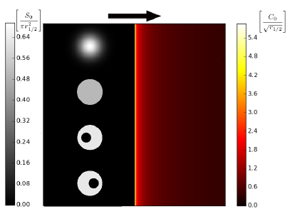
Figure 2: Source profiles for Gaussian, disk, crescents (right) and magnification map for an infinite fold (left). Objects have the same $S_{0}$ and $r_{1/2}$. The black arrow marks the direction of motion of the sources relative to the caustic.

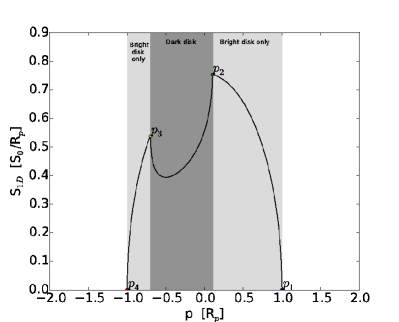
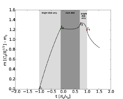
Figure 8: The characteristic points and instances of a crescent source’s one dimensional profile and microlensing lightcurve.

Section 4 shows the light curves that result when each of the model sources crosses an ideal fold. This would apply in Figure 1 to sources along the path AB or BC, for sources small enough that the curvature of the caustics is negligible. With this assumption one can imagine the caustic as an infinite wall to be crossed by the source as presented in Figure 2. The source brightness distribution parallel to the caustic naturally makes no difference to the observable brightness; each source can be replaced by an effective one-dimensional source profile, by flattening the source so it becomes perpendicular to the caustic. In principle, the effective one-dimensional brightness profile could be recovered from the light curve by deconvolution. Agol & Krolik (1999) modelled this profile as the result of a circular accretion disc seen through the spacetime around a Kerr black hole, and Abolmasov & Shakura (2012) have applied the idea to observed light curves to infer properties of quasar accretion discs. In this work, we take a simpler but arguably more robust approach: we study features in the light curves characteristic of a crescent-like source which in turn would indicate a black-hole silhouette. Figure 8 shows the qualitative features: there is a period during which the dark cutout disc is crossing the caustic, and before and after there are periods when the only the bright parts of the crescent are in transit across the caustic. The details depend on the orientation of the crescent, but basically the dark disc causes a rising light curve to plateau or dip. These features are still present, albeit faintly, if the simple crescent is replaced by a source based on an accretion-disc simulation of a black-hole environment (Figures LABEL:fig:M87_image–9).

In Section 5 we carry out source fitting to lightcurves, with both noise and systematic errors are present. We generate three lightcurves by taking a uniform disc, a circular Gaussian, and a crescent across the path AB in Figure 1, and then adding noise. The path simulates crossing a clean but not ideal fold. In addition, we generate templates lightcurves by running the three source types, with various parameter values, across the path CB. That is, the templates come from a similar but not identical caustic, thus deliberately generating a systematic error. We then fit the noisy lightcurves to the templates using Markov chain Monte-Carlo. We find that the correct source type can be inferred from the $\chi^{2}$ values. The parameter values can also be inferred. The fitting errors are larger than the formal uncertainties, which is expected in the presence of systematic errors, but still appear acceptable.

Finally in Section 6 we discuss in more depth the implications of the results presented in the previously mentioned sections. One of the most interesting implication is the possibility to estimate the black hole mass from the reconstructed parameters. This further requires good approximations of the relative transversal velocity between the quasar and the lens. Proper constraints can be set with independent observations of the stellar structure that contain the gravitational lens.

The thorough study of the possibility to reconstruct the quasar’s structural parameters from light-curves containing multiple microlensing events represents the target of future work. This will most probably require the use of powerful statistical tools. Another path for future work is the designing of an observation regime best suited for acquiring the necessary microlensed light-curve.

2 Microlensing

We start by introducing in a succinct manner the gravitational lensing theory that is relevant for microlensing in general and for the scope of the present paper in particular. More detailed presentation of the theory can be found in several references, such as Petters et al. (2001).

2.1 Magnification

The gravitational lens equation

$$\vec{\beta}=\vec{\theta}-\vec{\alpha}(\vec{\theta})$$ (1)

relates the apparent sky position $\vec{\theta}$ of a light source to its true but unobservable sky position $\vec{\beta}$ through the bending angle $\vec{\alpha}$. The latter is an integral

$$\vec{\alpha}=(1+z_{{}_{L}})\frac{D_{S}-D_{L}}{D_{S}D_{L}}\frac{4G}{c^{2}}\int\Sigma(\vec{\theta}^{\prime})\frac{\vec{\theta}-\vec{\theta}^{\prime}}{|\vec{\theta}-\vec{\theta}^{\prime}|^{2}}\,d^{2}\vec{\theta}^{\prime}$$ (2)

depending on the projected density $\Sigma(\vec{\theta})$ (kg/steradian) of the lens, the lens redshift $z_{{}_{L}}$ and the comoving distances $D_{L}$ and $D_{S}$ to the lens and source. The derivative of the apparent position with respect to the source position

$$M(\vec{\theta})=\left(\frac{\partial\beta}{\partial\theta}\right)^{-1}$$ (3)

is known as the magnification matrix, and its determinant

$$\mu(\vec{\theta})=\det|M(\vec{\theta})|$$ (4)

is the brightness amplification of an image of a point source. In other words, the source will brighten or dim according to whether $\mu(\vec{\theta})$ is more or less than unity. If there are multiple mages at distinct but not observationally resolved $\vec{\theta}_{i}$ from the same $\vec{\beta}$, a total brightness amplification of

$$\mu_{\rm total}=\sum_{i}\mu(\vec{\theta}_{i})$$ (5)

applies. It is possible for the magnification to become formally infinite, as a result of an eigenvalues of the magnification matrix (3) becoming infinite. This generically happens on curves on the $\vec{\theta}$ plane, known as critical curves. Mapping a critical curve to the source plane, through the lens equation (1), to the source plane $\vec{\beta}$ gives the so-called caustics. Caustics can appear in the optical system, not just gravitational lensing. For a point source, caustics are singularities of the magnification; for finite-size sources caustics correspond to high and sharply changing magnification.

Caustics are important in all forms of lensing with multiple images, but they have a special significance for lens quasars, first pointed out by Chang & Refsdal (1979). The granularity of the mass distribution $\Sigma(\vec{\theta})$ due to individual stars produces a caustic network on the scale of $\sqrt{GM_{\odot}D_{L}/c^{2}}$ or $10^{-6}\sqrt{M/M_{\odot}}\rm\,arcsec$ for typical lens and source redshift (Wambsganss, 2001). Extended sources wash out this micro-caustic structure, but the optical-continuum source of quasars is even smaller.

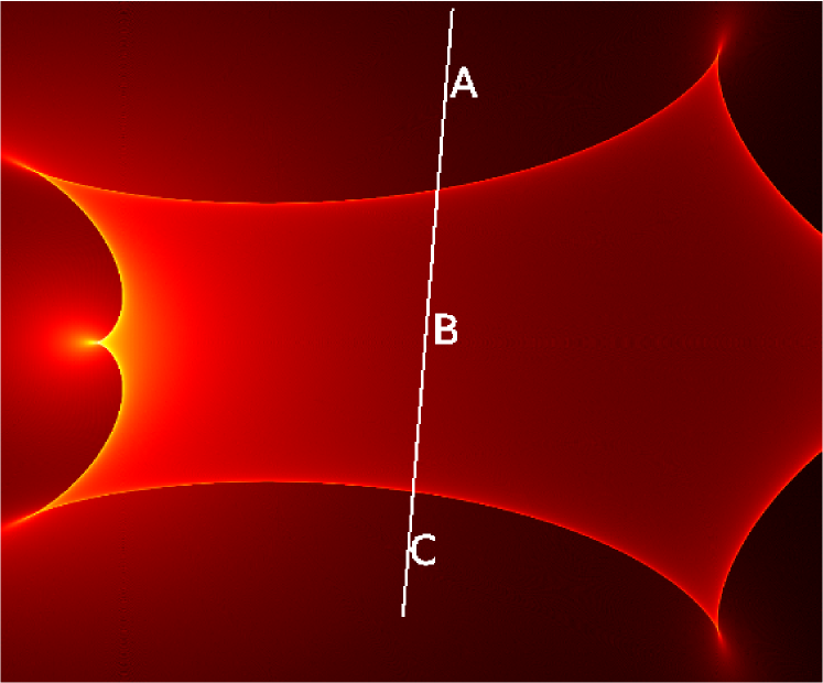
Figure 1: Magnification map used later in this paper (Section 5). The white line marks the trajectory of the center of the sources for which the lightcurves presented in figure 11 are generated. Note that this represents an atypically simple region of any realistic magnification map.

2.2 Magnification near a fold caustic

A simple example of a caustic network is shown in Figure 1. There are two general categories of caustics in gravitational lensing, cusps and fold, and examples of both kinds can be seen in this figure. Magnification near a caustic has universal properties, independent of the system and has been extensively studied (Blandford & Narayan, 1986; Schneider & Weiss, 1992; Gaudi & Petters, 2002a, b). In particular, at distance $p$ from a fold caustic

$$\mu(p)=\mu_{0}+C_{0}\frac{1}{\sqrt{p}}\Theta(p).$$ (6)

Here the magnification of a point source near a caustic is equal to the sum of the magnification due to other reasons $\mu_{0}$, assumed to be locally constant, and a decrease with the square root of the distance from the fold. The latter term becomes activated only after the source enters the region interior to the caustic curves when the values of the step function $\Theta(p)$ become unity. The proportionality constant $C_{0}$ depends on the local conditions in the vicinity of the caustic.

A source of arbitrary shape can be described by a two-dimensional brightness function $S_{2D}(p-p_{s},q-q_{s})$ defined for a coordinate system $p,q$ where $p_{s},q_{s}$ denote the coordinates of the center of a source.

For a microlensing event the lightcurve can be written for an undefined source shape as:

$$F(t)=\int_{-\infty}^{\infty}\int_{-\infty}^{\infty}S_{2D}(p-p_{s}(t),q-q_{s}(t))\mu_{t}(p)\mathrm{d}q\mathrm{d}p$$ (7)

In order to build the previous equation we have considered that the time dependency of the flux $F$ is given only by the motion of the source with respect to a fixed caustic. Therefore the only time dependent quantities in the right hand side of the equation are the coordinates of the center of the source $p_{s},q_{s}$ and by construct $S_{2D}$.

Due to the choice of the coordinate system the amplification factor has no dependence on the $q$ coordinate. The previous equation can be rewritten as:

$$F(t)=\int_{-\infty}^{\infty}\mu_{t}(p)S_{1D}\left(p-p_{s}(t)\right)\mathrm{d}p,$$ (8)

where we have defined the one dimensional flux function as:

$$S_{1D}(p-p_{s}(t))=\int_{-\infty}^{\infty}S_{2D}(p-p_{s}(t),q-q_{s}(t))\mathrm{d}q$$ (9)

This representation is a valid approximation only when the apparent size of the source is much smaller than the corresponding Einstein angle of the lens. In this context all the information about the source shape and brightness that can be contained in the lightcurve is exhaustively given by the 1D flux function. In other words, if two sources with different $S_{2D}$ have the same $S_{1D}$ they cannot be distinguished by studying their lightcurves.

3 Models for extended sources

In the present study we are analysing three types of sources with different surface brightness:

1. a rotationally symmetric source with a bivariate gaussian surface brightness distribution,

2. a disk source with constant surface brightness distribution,

3. a crescent shaped source with constant surface brightness distribution.

The first two sources are the typical choices used in the literature to describe the luminous parts of a quasar (Prasenjit should give some citations here). The third one is a recently proposed variant (Kamruddin & Dexter, 2013).

3.1 Rotationally symmetric source with a bivariate gaussian surface brightness distribution

A symmetric 2D gaussian can be described mathematically as:

$$S_{2D}^{G}(p-p_{s},q-q_{s})=\frac{S_{0}^{G}}{2\pi\sigma^{2}}e^{-\frac{(p-p_{s})^{2}}{2\sigma^{2}}}e^{-\frac{(q-q_{s})^{2}}{2\sigma^{2}}}.$$ (10)

The corresponding 1D brightness is:

$$S_{1D}^{G}(p-p_{s})=\frac{S_{0}^{G}}{\sqrt{2\pi}\sigma}e^{-\frac{(p-p_{s})^{2}}{2\sigma^{2}}}.$$ (11)

Other parameters of the model are the total flux $S_{0}^{G}$ and $\sigma$.

Although such a definition for a source would have non-zero surface/linear brightness for any coordinate $p,q$, the amount of light received by a detector from outside a $3\sigma$ disk centered at $p_{s},q_{s}$ would be insignificant. For a gaussian distributed surface brightness source the half-light radius is directly proportional to the parameter $\sigma$ according to the equation:

$$r_{1/2}=\sqrt{ln(4)}\sigma.$$ (12)

3.2 Disk source with constant surface brightness distribution

One can construct mathematically a disk source with constant surface brightness and radius $R$ using a stepfunction:

$$S_{2D}^{D}(p-p_{s},q-q_{s})=\frac{S_{0}^{D}}{\pi R^{2}}\Theta\left(R^{2}-\left(p-p_{s}\right)^{2}-\left(q-q_{s}\right)^{2}\right).$$ (13)

By integrating over $q$ coordinate the linear brightness function is obtained:

$$S_{1D}^{D}(p-p_{s})=\frac{2S_{0}^{D}}{\pi R}\sqrt{1-\frac{(p-p_{s})^{2}}{R^{2}}}\Theta\left(R^{2}-\left(p-p_{s}\right)^{2}\right).$$ (14)

The half-light radius of a uniform disk source is $R/\sqrt{2}$.

3.3 Crescent source with constant surface brightness distribution

The surface brightness distribution of a geometric crescent can be built by considering two disk sources of constant brightness. One larger disk will contribute positively to the total flux while one smaller disk that is interior to the large one will contribute negatively. This superposition can be written for 2D as:

$$S_{2D}^{C}=S_{2D}^{Dp}-S_{2D}^{Dn}$$ (15)

with

$$S_{2D}^{Dp}(p-p_{sn},q-q_{sn})=\frac{S_{0}^{Dp}}{\pi R_{p}^{2}}\Theta\left(R_{p}^{2}-\left(p-p_{sp}\right)^{2}-\left(q-q_{sp}\right)^{2}\right)$$ (16)

and

$$S_{2D}^{Dn}(p-p_{sn},q-q_{sn})=\frac{S_{0}^{Dn}}{\pi R_{n}^{2}}\Theta\left(R_{n}^{2}-\left(p-p_{sn}\right)^{2}-\left(q-q_{sn}\right)^{2}\right).$$ (17)

The following notations were used: $R_{p},(p_{sp},q_{sp}),R_{n},(p_{sn},q_{sn})$ are the radii and coordinate of the center for the larger positive disk and smaller negative disk respectively. $S_{0}^{Dp},S_{0}^{Dn}$ represent the total flux of radiation received from the large and small disk. From this point forward we will not use the total flux from each source. Instead we will use the difference which in this case is th total flux from the crescent-shaped source $S_{0}^{C}$.
Equation 15 can be written as:

$$S_{2D}^{C} =\frac{S_{0}^{C}}{\pi\left(R_{p}^{2}-R_{n}^{2}\right)}\left\{\Theta\left[R_{p}^{2}-\left(p-p_{sp}\right)^{2}-\left(q-q_{sp}\right)^{2}\right]\right.$$

$$\qquad\left.{}-\Theta\left[R_{n}^{2}-\left(p-p_{sn}\right)^{2}-\left(q-q_{sn}\right)^{2}\right]\right\}.$$ (18)

Analogous for the linear brightness function:

$$S_{1D}^{C} =\frac{2S_{0}^{C}}{\pi\left(R_{p}^{2}-R_{n}^{2}\right)}\left\{\sqrt{R_{p}^{2}-(p-p_{sp})^{2}}\Theta\left[R_{p}^{2}-\left(p-p_{sp}\right)^{2}\right]\right.$$

$$\qquad\left.{}-\sqrt{R_{n}^{2}-(p-p_{sn})^{2}}\Theta\left[R_{n}^{2}-\left(p-p_{sn}\right)^{2}\right]\right\}.$$ (19)

There are some constraints on the parameters used to define a crescent in the previously presented manner that need to be stated. First, we must impose the obvious $R_{p}>R_{n}$ relation. Secondly, the small disk must always be interior to the large disk:

$$R_{p}\geq R_{n}+\sqrt{\left(p_{sp}-p_{sn}\right)^{2}+\left(q_{sp}-q_{sn}\right)^{2}}$$ (20)

For the distances between the centers of the two disks we will use the same notations as the one found in the paper (Kamruddin & Dexter, 2013), $a\equiv p_{sn}-p_{sp}$ and $b\equiv q_{sn}-q_{sp}$.

The half-light radius of any source is invariant to any rotational transformation. In the present case of a crescent source the effective radius is dependent on the parameters $R_{p}$, $R_{n}$ and $\sqrt{a^{2}+b^{2}}\equiv c$ exclusively. From symmetry considerations the centroid of the source is collinear with the centers of the two disks and it is situated at a distance $d_{c}$ from the center of the bright disk. $d_{c}$ can be computed numerically with the use of a variation of equation 19:

$$\frac{S_{0}^{C}}{2} =\frac{2S_{0}^{C}}{\pi\left(R_{p}^{2}-R_{n}^{2}\right)}\int_{d_{c}}^{R_{p}}\bigg{[}\sqrt{R_{p}^{2}-p^{2}}$$ (21)

$$-\sqrt{R_{p}^{2}-\left(p-c\right)^{2}}\Theta\left(R_{p}^{2}-\left(p-c\right)^{2}\right)\bigg{]}dp.$$

With the position of the centroid determined, the half-light radius can be also be computed numerically:

$$S_{0}^{C} =\frac{4S_{0}^{C}}{\pi\left(R_{p}^{2}-R_{n}^{2}\right)}\int_{0}^{r_{1/2}}\left[\Theta_{2}-\Theta_{1}\right]pdp;$$ (22)

$$\Theta_{1} =\bigg{[}\pi-\arccos\frac{R_{p}^{2}+p^{2}-d_{c}^{2}}{2R_{p}p}$$

$$\phantom{=\bigg{[}\pi}-\arccos\frac{R_{p}^{2}-p^{2}+d_{c}^{2}}{2R_{p}d_{c}}\bigg{]}\Theta\left(p-R_{p}+d_{c}\right);$$

$$\Theta_{2} =\pi-\arccos\frac{p^{2}+(c+d_{c})^{2}-R_{n}^{2}}{2p\left(c+d_{c}\right)}$$

$$\phantom{=\pi-}\Theta\left(p+R_{n}-d_{c}-c\right).$$

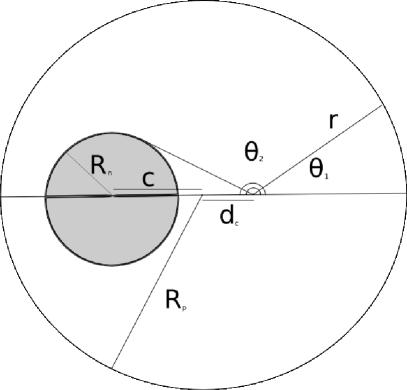
Figure 3: Geometry of crescent sources.

4 Lightcurves of the extended sources during fold crossing

Using equation 8 and the one-dimensional flux function presented in the previous section one can compute numerically the lightcurves of the three extended sources for the simplified infinite-wall-caustics model.

4.1 Lightcurve of the gaussian source

The amount of light received by an observer from a source with a gaussian distributed brightness with $\sigma$ and total flux $S_{0}^{G}$ in the absence of any gravitational lensing is:

$$F^{G}(t)=\int_{-\infty}^{\infty}\left(\mu_{0}+\frac{C_{0}}{\sqrt{p}}\Theta\left(p\right)\right)\left(\frac{S_{0}^{G}}{\sqrt{2\pi}\sigma}e^{-\frac{(p-p_{s}(t))^{2}}{2\sigma^{2}}}\right)\mathrm{d}p.$$ (23)

which can be simplified to:

$$F^{G}(t)=\mu_{0}S_{0}^{G}+\frac{C_{0}S_{0}^{G}}{\sqrt{2\pi}\sigma}\int_{0}^{\infty}\frac{e^{-\frac{(p-p_{s}(t))^{2}}{2\sigma^{2}}}}{\sqrt{p}}\mathrm{d}p.$$ (24)

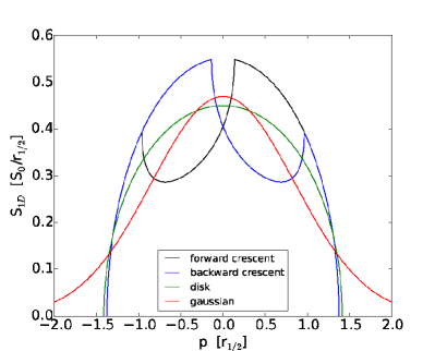
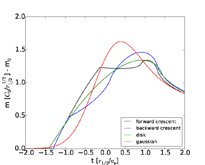
Figure 4: Lightcurves of crescents, Gaussian and disk for sources with identical $S_{0}$ and $r_{1/2}$. Crescent source has $r_{1/2}$ = 0.72754 $R_{p}$, $R_{n}$ = 0.4 $R_{p}$, a = 0.3/-0.3 $R_{p}$

4.2 Lightcurve of the disk shaped source

Analogous to the gaussian shaped source, the disk source with uniform brightness, radius $R$ and unmagnified flux $S_{0}^{D}$ has a lightcurve described by the equation:

$$F^{D}(t) =\int_{-\infty}^{\infty}\left(\mu_{0}+\frac{C_{0}}{\sqrt{p}}\Theta\left(p\right)\right)$$ (25)

$$\bigg{[}\frac{2S_{0}^{D}}{\pi R}\sqrt{1-\frac{\left(p-p_{s}(t)\right)^{2}}{R^{2}}}\Theta\left(R^{2}-\left(p-p_{s}(t)\right)^{2}\right)\bigg{]}\mathrm{d}p.$$

which is equivalent to:

$$F^{D}(t)=\mu_{0}S_{0}^{D}+\frac{2C_{0}S_{0}^{D}}{\pi R}\int_{max(0,p_{s}(t)-R)}^{max(0,p_{s}(t)+R)}\frac{1}{\sqrt{p}}\sqrt{1-\frac{\left(p-p_{s}(t)\right)^{2}}{R^{2}}}\mathrm{d}p.$$ (26)

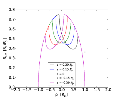
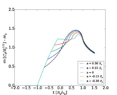
Figure 5: Lightcurves of crescent sources with $R_{n}$ = 0.4 $R_{p}$.

4.3 Lightcurve of the crescent shaped source

The lightcurve of a crescent shaped source with unamplified flux $S_{0}^{C}$, radii $R_{p}$, $R_{n}$ and center displacement $a(t)$ is:

$$F^{c}(t) =\mu_{0}S_{0}^{C}+C_{0}\frac{2S_{0}^{C}}{\pi\left(R_{p}^{2}-R_{n}^{2}\right)}$$ (27)

$$\bigg{[}\int_{max(0,p_{s}(t)-R)}^{max(0,p_{s}(t)+R)}\sqrt{\frac{R_{p}^{2}-\left(p-p_{s}(t)\right)^{2}}{p}}\mathrm{d}p$$

$$-\int_{max(0,p_{s}(t)-a(t)-R)}^{max(0,p_{s}(t)-a(t)+R)}\sqrt{\frac{R_{p}^{2}-\left(p-p_{s}(t)+a(t)\right)^{2}}{p}}\mathrm{d}p\bigg{]}.$$

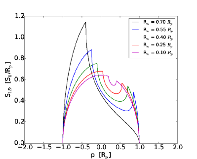
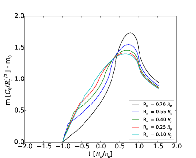
Figure 6: Lightcurves of backwards crescents with a = 0.3 $R_{p}$.

The function $p_{s}(t)$ can be chosen to be equal to $v_{p}(t-t_{0})+p_{s0}$. Where $p_{s0}$ is the coordinate $p$ of the source at the initial time, and $v_{p}$ is the component of the velocity along the $p$ axis. Such a modelling of the motion of the object in the source plane describes a linear motion with constant velocity. Furthermore, we reduce the complexity of the model by choosing the function $a(t)$ to be constant in time.

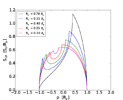
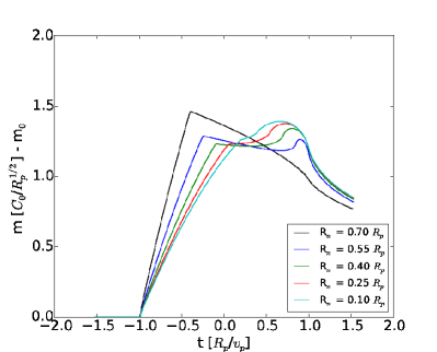
Figure 7: Lightcurve of forwards crescents with a = -0.3 $R_{p}$.

There are four characteristic points visible on the resulting one-dimensional light profile of the crescent shaped source. Two of the points, p1 and p4, mark the outer boundaries of the luminous disc component. The other two, p2 and p3, mark the boundaries of the dark disc component. Since $S_{1D}$ is a projection of $S_{2D}$ on a line perpendicular to the caustic, the following relation holds:

$$p_{2}-p_{1}=R_{p}-R_{n}-a.$$ (28)

In addition there are two other obvious relations the characteristic points which are independent of the projection:

$$p_{4}-p_{1}=2R_{p},$$ (29)

$$p_{3}-p_{2}=2R_{n}.$$ (30)

All four points mark the positions where derivative $\frac{dS_{1D}}{dp}$ is discontinuous. The points can be used to define three regions: $p_{1}-p_{2}$ where $S_{1}D$ is convex, $p_{2}-p_{3}$ where $S_{1}D$ is concave, and $p_{3}-p_{4}$ where $S_{1}D$ is convex again.

Due to the nature of the caustic and the monotonic behaviour of the magnification map on both sides of the caustic. The previously mentioned characteristic points are inherited by the microlensing lightcurve. The points on the temporal dimension $t_{1},t_{2},t_{3}$ and $t_{4}$ correspond to instances in time when the fold is aligned with $p_{1},p_{2},p_{3}$ and $p_{4}$, respectively. For a constant relative velocity $v_{p}$ between the source and the caustic there is a simple relation between the points $p_{i}$ and instances $t_{i}$:

$$t_{j}-t_{i}=\frac{p_{j}-p_{i}}{v_{p}}.$$ (31)

With the use of the previous four equations the following identities can be written:

$$R_{p}=\frac{v_{p}\left(t_{4}-t_{1}\right)}{2},$$ (32)

$$R_{n}=\frac{v_{p}\left(t_{3}-t_{2}\right)}{2},$$ (33)

$$a=\frac{v_{p}\left(t_{4}+t_{1}-t_{3}-t_{2}\right)}{2}.$$ (34)

Figure 4 reveals that the lightcurve of a crescent source has more visible features than the other two light-curves corresponding to the disc and gaussian shape. There are three regions where $S_{1D}$ and by inheritance, the lightcurve has distinguishable behaviour. The first region that would be recorded on a lightcurve plot represents the period of time when the bright disk begins to be overlapped by the caustic and stops when just before the dark disk reaches the caustic. During this period of time, the flux of light from the source is increasingly magnified. The second period starts and ends with the overlapping of the dark disc. As a boundary of the two regions, there is a distinguishable point where the slope of the magnification is drastically changed. This apparent discontinuity in the first derivative of the magnification function is caused by the caustic amplification of the sudden drop in the $S_{1d}$ function. During the respective period, the magnification growth slows or even reverses during the first part of the period and starts to grow faster again as the dark disk ends its overlap with the caustic. At the point where the dark disc clears the caustic, the growth of the magnification is infinite, which appears as a saddle point on the lightcurve. Next, the final period corresponds to the case when the dark disc has cleared the caustic and the bright disc continues to overlap with the caustic. During this period, the lightcurve reaches a peak that for most of the parameter space is global and for the rest of the parameter space local. At the end of the period, the growth of the magnification is negative infinite. the respective point appears as a second saddle point on the lightcurve. Past this point the magnification of any finite source will decay in roughly the same manner.

The impact of parameter $a$ on the shape of the lightcurve can be observed in figure 5 (a-var). Sources where the center of the dark disc reaches the caustic before the center of the bright disc are characterized by a smoother broad peak in contrast to the cases where the center of the dark disc reaches the caustic after the bright disk. In the case of the latter the instance when the dark disc reaches the caustic corresponds to larger and larger magnifications until it becomes a local and even global peak. The effect of the $R_{n}$ parameter on the light curve is presented in figures 6 and 7. For the particular set of parameters where $R_{p}=R_{n}+a$ the third period of time discussed previously does not exist. Particularizing further, if the value of the radius of the dark disc is comparable to the value of the radius of the bright one then the position and shape of the maximum magnification are strikingly different. In case the crescent reaches the caustic with the bright region first, the peak magnification happens when the dark region reaches the caustic and it is characterized by a sharp variation in magnification growth, In the opposite case, the peak appears before the end of the bright disc reaches the caustic and shape is smoother.

4.4 Microlensing a simulated image of M87

Dexter et al. (2012) have created a radiative image of M87 based on the GRMHD simulations presented in (McKinney & Blandford, 2009). The top right-most image in figure 5 of Dexter et al. (2012) has been projected to a 1D profile associated to the perpendicular direction to a fold caustic approaching the image from the right. The projection is presented in the upper panel of figure 9. The amplification values of the flux of light corresponding to a microlensing event are presented in the lower panel of figure 9. In general, the behaviour of the lightcurve is similar to the geometric crescent source with the caveat that the outer regions surrounding the luminous parts of the image have non-zero flux and thus are more extended than the simplified source model.

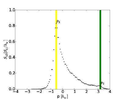
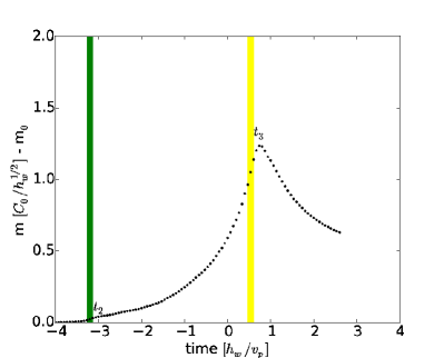
Figure 9: The one dimensional profile obtained from the numerical integration along the ordonata axis of the source image is presented in the upper panel. The corresponding lightcurve associated to the 1D profile is presented in the lower panel. The points p2 and p3 mark the start and end of the equivalent dark disk and are associated with the moments of their overlap with the caustic: t2 and t3.

5 Fitting mock data

Having used the simple model of an ideal fold to gain insight, we now move to the numerical computation of microlensing light curves with realistic mass distributions, and then fit source models to lightcurves in the presence of random and systematic errors.

First we generate microlensing magnification maps using the microlensing code created by Joachim Wambsganss (Wambsganss et al., 1999; Wambsganss, 1990, 1999). We then generate mock light curves for three source models — a crescent, a uniform disc and a Gaussian disc — and then fit each mock light curve to all three source models. Parameter fitting and marginalising was done by Markov-chain Monte Carlo (MCMC).

5.1 Numerical microlensing magnification maps

The code uses a ray-shooting technique to compute the gravitational lensing effect of a mass distribution consisting of (a) a smooth component and (b) a random distribution of point masses representing stars. The ray shooting maps a grid of $\vec{\theta}$ to $\vec{\beta}$ using the lens equation (1). That is, the rays are shot from the observer back to the source.

For the computation of the individual deflection angles $\vec{\alpha}(\vec{\theta})$ a hierarchical or tree method is used. The positions of all lensing masses are put into a grid of $\vec{\theta}$. Each grid cell is subdivided into four smaller squares recursively until every cell contains only one mass. Nearby masses are added individually while distance masses are clumped into larger grid cells whose net contribution is approximated by its first few multipole moments. Scaled units are used, with the constant pre-factor in the deflection angle (2) separated out.

The result of ray shooting is a pixel map on the $\vec{\beta}$ plane of the number of lightrays which arrive at the source plane from a particular observer. This intermediate result is effectively a magnification map on the source plane. Once the map is created, the lightcurve can be obtained by specifying the transit path of the source across the map. At each point on this transit line, the code computes equation (7) convolving the brightness distribution of the source with the magnification pattern of the map. In real life, not only are both lens and source moving but the lens lens configuration, and with it the magnification pattern, is also changing with time. While the first subtlety is taken care of by a coordinate transformation in this analysis, for the second one the lens configuration is assumed to be constant in time.

When generating the magnification map depicted in Figure 1, which is used in our analysis below, only two point masses were included. This was done in order to have clean fold caustics. For the computation of the actual lightcurve, the code was modified to also allow for crescent shaped images specified through the parameter set $R_{p},R_{n},a,b$. Here $R_{p}$ denotes the outer radius of the crescent and $R_{n}$ the inner one. The orientation of the source image with respect to the magnification map is specified by the parameters $a$ and $b$ as the shift of the center of the inner disk from the center of the outer disk in $x$- and $y$-direction respectively. In the original version of the code, gaussian and disk-shaped images were already implemented. Those are completely characterised by the single parameter $R_{p}$. The values of the parameters are specified in pixel units corresponding to the magnification map. Further, one needs to specify the start and end point coordinates of the path, which the center of the source image follows through the magnification map (see the depiction in figure 1). Hence, the points along this path are specified through the number of time steps for which the computation of the brightness is to be carried out. Those points correspond to the actual measurement of the brightness of an object in the observational case. For each timestep the two-dimensional convolution of equation 7 is carried out numerically for the position of the source on the magnification map.

For the purpose of this analysis, it was desirable to mimic the analytical behaviour of a simple fold as much as possible, for comparing the numerical result with the analytical one, therefore, the path of the source was chosen, so that it intersects the border of the caustic perpendicularly, and on a point where the border is a fold caustic.

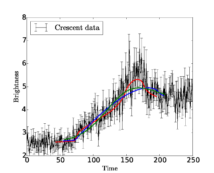
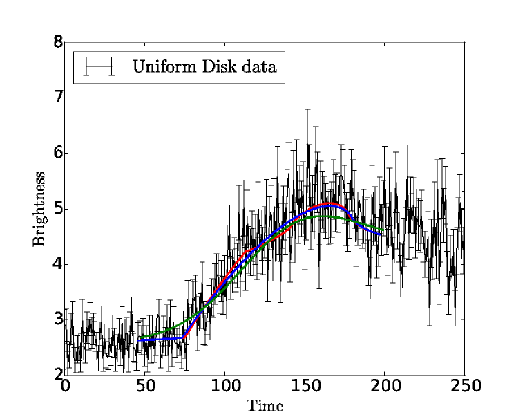
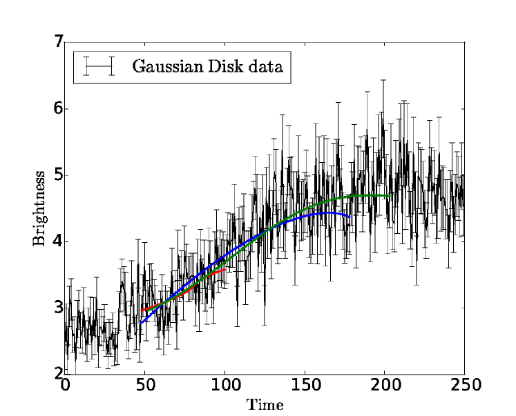
Figure 10: Three different mock datasets with three different parametrizations fitted to each — crescent (red), uniform-disk (blue) and Gaussian disk (green).

5.2 Mock light curves

Mock light curves were generated by running a source across a caustic, specifically along the line from point C to point B in Figure 1. The model light curves, to which these are fitted, are made by running a source across a different caustic, along the line from point A to point B in the same figure. That is, the mock data are generated with a clean but not ideal fold caustic and then fitted with another such caustic. This mimics the unavoidable systematic error of not knowing the caustic exactly.

The crescent source had parameters (as explained in §3.3) $R_{p}$ and $R_{n}$ being the radii of the outer and inner circles and $(\alpha,\beta)$ being the coordinates of the inner circle with respect to the centre of the outer circle in the coordinate system associated with the image in Figure 1 and not associated with the caustic surface as defined in the previous sections. The parameter values were

$$(R_{p},R_{n},\alpha,\beta)=(50.0,30.0,15.0,10.0).$$ (35)

The uniform disc had the same (outer) radius as the crescent. In the Gaussian source, we set $3\sigma=50$. For convenience, below we will refer to $R_{p}$ of the Gaussian source, by which we actually mean $3\sigma$.

Each mock light curve also has three nuisance parameters, namely the beginning and end of the event and the brightness normalisation. These are to be marginalised out by the MCMC.

Figure 10 shows the three light curves. Each has 250 points regularly spaced in time, with Gaussian noise at the level of 10% of the current brightness. This amounts formally to a single summary data point with a signal to noise of $10\times\sqrt{250}\simeq 160$.

5.3 Model fitting and likelihood analysis

Each of the three mock light curves was fitted to all three models. We denote the nine possible cases with letter pairs, with the first letter denoting the assumed model for the fitting procedure and the second letter representing the source: thus CG means a Crescent model was fitted to mock data from a Gaussian source, DC stands for a uniform Disc model fitted to mock data from a Crescent source, and so on.

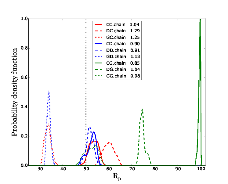
Figure 11: Posterior probability distribution for the source size $R_{p}$. The vertical line is the correct value. Same color represents the same dataset whereas same line style corresponds to same model fit. The legend gives the reduced $\chi^{2}$ of the best fit in each case.

Figure 11 shows the posterior probability distribution of $R_{p}$ for all nine cases, along with the minimum reduced $\chi^{2}$ for each case. The area under each curve is unity. Note that the height of the curves are not the likelihood, they are probability densities in parameter space.

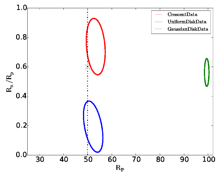
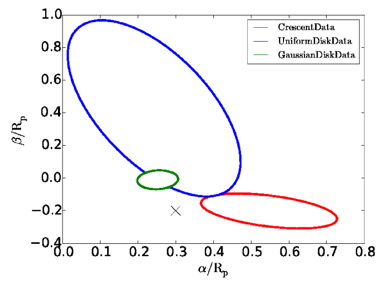
Figure 12: The 2$\sigma$ contours (or error ellipses) of the crescent model when fitting with the three different datasets.

Let us first consider the three cases where a crescent model was fitted. These are the solid curves in Figure 11, with the colours of the curves indicating the source. Meanwhile, Figure 12 shows $2\sigma$ of the inferred parameter values.

1. solid red curve in Figure 11 and red ellipses in Figure 12. In this case, a light curve from a crescent source was being fitted to a crescent model. The fit gives reduced $\chi^{2}$ close to unity, as expected. The recovered parameter values are near or slightly outside the $2\sigma$ ellipses. This is expected since we added a small systematic error, by using different caustics (though both clean folds) for the mock data and the model fit. The apparent degeneracy between $a$ and $b$, seen in Figure 12, is also expected, since only the distance of the crescent’s small circle from the caustic influences the magnification.

2. solid blue curve and blue ellipses. Here a crescent model was fitted to a light curve from a uniform disc. The situation is formally a crescent with $R_{n}=0$ and $a,b$ arbitrary, and this shows in the blue ellipses in the recovered parameter values. The redundant parameters $\alpha$ and $\beta$, in effect, allow the model to partly fit the noise, and hence, the $\chi^{2}$ is somewhat lower than in the previous case.

   

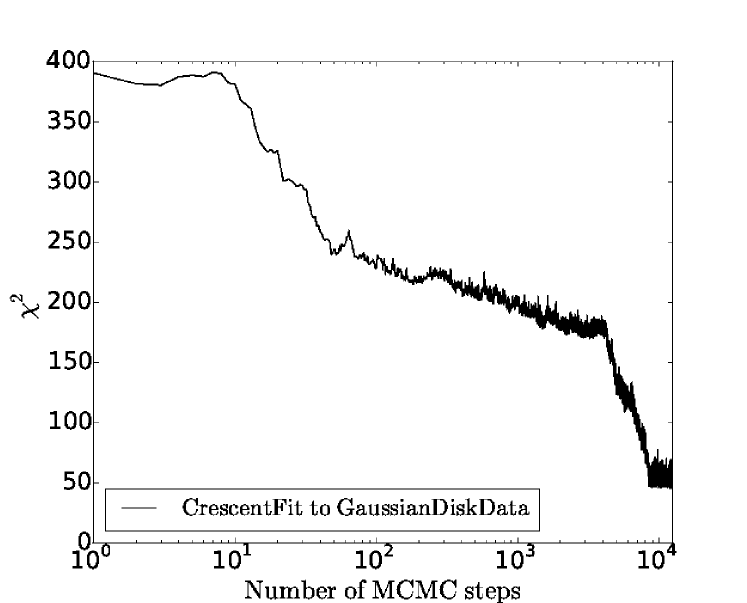
   Figure 13: The $\chi^{2}$ of each step of the full MCMC for one case.

3. Solid green curve and green ellipses. Additionally, Figure 13 shows the progress of reduction of $\chi^{2}$ in this case, where a crescent-source model is used to fit data from a Gaussian source. The parameter values are seemingly tightly constrained, but the recovered $R_{p}$ is completely wrong since the correct value is far from the green curve and green ellipses. The reduced $\chi^{2}$ is only 0.85, indicative of over-fitting. We can see what has happened from the red curve in the bottom panel of Figure 10. The best-fit model covers only a small part of the light curve. That is, the fitting procedure has exploited the nuisance parameters to find a good fit to mainly noise.

Next we consider the three cases where a disc model is fitted. These correspond to the dashed curves in Figure 11. There is only one interesting parameter to fit, the disc radius $R_{p}$, and no equivalent of Figure 12 is needed.

1. red dashed curve. On fitting a disc model to a crescent-source source, the recovered $R_{p}$ is incorrect, but the reduced $\chi^{2}$ of 1.29 signals that the data reject the model.

2. blue dashed curve. When the correct model is fitted to a disc-source, the best fit $\chi^{2}=0.91$ is good and $R_{p}$ is recovered within the uncertainty estimate.

3. green dashed curve. On fitting a disc model to a Gaussian-source model, the recovered $R_{p}$ is incorrect, but the reduced $\chi^{2}$ gives no signal that something is amiss. It appears that a Gaussian source could mimic a uniform disc.

Finally, we consider the three cases where a Gaussian model is fitted. These correspond to the dotted curves in Figure 11. Again, there is only one interesting parameter to fit, the Gaussian $3\sigma$-radius, which we have called $R_{p}$.

1. red dotted curve. When a Gaussian-source model is fitted to data from a crescent source, the recovered $R_{p}$ is wrong but the reduced $\chi^{2}=1.29$ shows the data rejecting the model.

2. blue dotted curve. When a Gaussian-source model is fitted to data from a uniform disc, the recovered $R_{p}$ is wrong but the model is rejected anyway.

3. green dotted curve. When data from a Gaussian is fitted to the correct model, $R_{p}$ is recovered within it’s estimated uncertainty and the best fit reduced $\chi^{2}$ is close to unity.

The above results suggest the following strategy for fitting a lightcurve from an unknown source profile: first try a Gaussian-source model; if the data reject that model, try a uniform disc; if the uniform disc is also rejected by the data, try a crescent model. Our numerical experiments indicate — assuming one of the three sources models are correct — that the reduced $\chi^{2}$ would unmask the correct model, and its parameters would be correctly recovered.

6 Discussion

In the current paper, we simulate and study the resulting microlensing lightcurves of geometric crescent-shaped sources and compare them with the microlensing lightcurves of other simple mathematically describable source profiles. In order to mimic the behaviour of the flux of light from the source in the proximity of a fold caustic, we make use of the simple approximation described in equation (5). The equation would exhaustively describe the magnification map and offer a good universal approximation for the particular microlensing regime that we consider. Namely, the shape of the caustic boundary in the proximity of the source in the respective plane can be approximated by a line due to reason that the local radius of curvature of caustic is orders of magnitude greater than the half-light radius of the studied source. In particular cases in which the previously mentioned approximation loses its validity, the impact on the quality of the lightcurves is not evenly distributed. The shape of the lightcurve will be maintained. The data points corresponding to the source position before and during the overlapping of the caustic will be affected by smaller errors than the data points corresponding to later times.

The first two source profiles that we consider are the uniform disk and symmetric Gaussian source. Both of them can be described by a half-light radius $r_{1/2}$ and a total unlensed light flux $S_{0}$. With the two parameters constrained the one-dimensional profiles, as well as the lightcurves of the two source, are completely determined, since no free parameter remains.

The previous statement does not hold for a crescent source. In the case of the crescent source there are in total five parameters: the integrated flux of the source $S_{0}$, the radii of the bright/dark disk $R_{p}$/$R_{n}$ and the displacement of the centers of the two disks on the axes perpendicular and parallel to the caustic $a$ and $b$.

Two of the parameters can be reduced by expressing the results in terms of $S_{0}$ and $r_{1/2}$. The later being determinable for any set of parameters $R_{p},R_{n}$ and $a^{2}+b^{2}$. Moreover, one of the displacement parameters $b$ has no impact on the one-dimensional profile of the source that results from the projection of the source image on an axis perpendicular to the caustic.

Since the one-dimensional source profile that corresponds to an axis perpendicular to the caustic contains exhaustively all the information regarding the source that can be revealed by the lightcurve, the value of the parameter $b$ does not have an effect on the shape of the lightcurve.

Nevertheless, the $b$ parameter is relevant for the calculation of $r_{1/2}$. It’s qualitative effect is to decrease the value of the half-light radius when the absolute value of the parameter is increased. With two parameters constrained and another irrelevant to the shape of the lightcurve, two free parameters remain $R_{n}$ and $a$. Figure 4 reveals that the lightcurve of a crescent source has more visible features than the other two light-curves corresponding to the disc and Gaussian shape. The parameters $R_{n}$ and $a$ have strong influences on the shape of the microlensed lightcurve as can be seen in figures 5, 6 and 7. Moreover, the one-dimensional source profile corresponding to the direction perpendicular to the caustic reveal four characteristic points. The overlap of each of these points with the caustic leaves visible features on the lightcurve at the corresponding instances of time. In timely order, the instances correspond to the start of the overlap between the caustic and the bright disk, the start of the overlap between the caustic and the dark disk, the end of the overlap between the caustic and dark disk and finally the end of the overlap between the caustic and the bright disk.

With the different source profiles and their corresponding lightcurves studied we can change our point of view of the system to that of an observer. The observer would basically detect only the lightcurve of such a source. As described in section 4.3 the timing of the onset and offset of the previously described periods can be used to estimate the values of the radii and one of the displacement parameters when assuming a geometric crescent. All quantities can be estimated in terms of the relative velocity of the source in a direction perpendicular to the caustic.

Furthermore, a simulated image of M87 presented in (Dexter et al., 2012) has been microlensed (figure 9). On the resulting lightcurve the instances corresponding to the start and end of the black hole shadow and caustic overlap were distinguishable.

In the case of a high-quality lightcurve with insignificant noise and measurement errors, the parameters can be obtained by simply identifying the characteristic instances of time without making use of the actual values of the magnification map. If the effect of the errors and the noise distorts the magnification time function enough so that the characteristic epochs are not identifiable with the characteristic periods still visible, the boundaries of the periods can be roughly estimated. Furthermore, if direct estimates of the parameters cannot be obtained we propose the use of a strong statistical tool such as Markov-Chain Monte Carlo. In Section 6 we have studied the possibility of identifying a crescent source and the possibility of recovering the respective parameters. As magnification map, we have used a complex numerical one generated with the microlensing code by Wambsganss et al. (1999). In addition, we have added to the signal a Gaussian noise with an SNR of 1.6. In the experiment, we have considered all nine combinations of original source profiles and assumed fitting source models. Effectively we have fitted using MCMC all three sources with all three assumed fitting models. The results of the experiment allowed us to build a procedure for distinguishing the shape of the source assuming that one of the three models we have considered is a good approximation. The procedure would be useful for observers that endeavour to gain more information about an unresolved source for which they can study the microlensing lightcurve. As a first step in the procedure, one should first attempt to use MCMC with a Gaussian model assumption. If either the value of the $\chi^{2}$ or the number of rejected datapoints is large then the next step is to change the assumed source model to a uniform disc and redo the fitting. Finally, if the uniform disc assumption is rejected as well then the fitting should be done with a crescent source model assumption. If at each of the three steps the data rejects the model then the source cannot be approximated by any of the three models. Otherwise, if at one of the steps the data does not reject the model then the respective model is a good approximation.

The previously mentioned abstract parameters can be related to physical quantities specific to the central region of a quasar. As such the luminous region would correspond to the bright accretion disc that surrounds the black hole. The later’s gravity would cause a shadow in the bright region limited by the extent of the event horizon of the black hole. Therefore, the radius of the bright disk would provide an estimate of the size of the accretion disk and the radius of the dark disc would provide and estimate of the gravitationally magnified Schwarzschild radius of the black hole $R_{S}^{magnified}=\Delta t_{dark}\cdot v_{p}$. By $R_{S}^{magnified}$ we refer to the apparent Schwarzschild radius which is larger than the real value at large distances due to the black hole’s own gravity. Moreover, the gravitationally magnified value of the Schwarzschild radius is a monotonic function of the black hole’s mass. Therefore, it can be used to estimate the mass of the black hole if it was not rotating. In the previous expression, the $\Delta t_{dark}$ denotes the period of overlap between the black hole shadow and fold caustic. $v_{p}$ denotes the component of the relative velocity of the source and fold which is perpendicular to the caustic. The respective velocity is an unknown, though it can be constrained on a case by case basis to an order of magnitude or even better. This would require the study of the dynamics of the stellar structure which contains the gravitational lens. A better estimate of the relative velocity would facilitate a better estimate of the effective non-rotating black hole mass associated with the black hole shadow.

The parameters whose values cannot be determined due to the loss of information from the directions parallel to the caustic could be obtained in the eventuality in which the same source crosses multiple caustics that are not parallel. Multiple crossing of caustics can reveal details of the one-dimensional flux profile corresponding to multiple distinct directions which would allow the reconstruction of the two-dimensional profile analogous to the process through which an image of a CT scan is obtained.

Author contributions
Prasenjit Saha provided the original idea and plan for the research project as well as multiple contributions to the analysis and manuscript preparation. Mihai Tomozeiu simulated and studied the ideal behaviour of the microlensing lightcurves for the different source profiles discussed and prepared the manuscript. Joachim Wambsganss contributed to the research planning and provided the numerical code used by Manuel Rabold to create the magnification map and corresponding lightcurves used in the MCMC analysis performed by Irshad Mohammed in the last part of the presented work. Both Manuel Rabold and Irshad Mohammed had large contributions in writing the ”Fitting Mock Data” section.

7 Acknowledgement

IM is supported by Fermi Research Alliance, LLC under Contract No. De-AC02-07CH11359 with the United States Department of Energy. J.W. would like to acknowledge and thank the Pauli Center for Theoretical Studies of ETH Zurich and University of Zurich for generous support during the Schrödinger visiting professorship in 2013.

References

- Abolmasov & Shakura (2012) Abolmasov P., Shakura N. I., 2012, MNRAS, 423, 676
- Agol & Krolik (1999) Agol E., Krolik J., 1999, ApJ, 524, 49
- Begelman et al. (1984) Begelman M. C., Blandford R. D., Rees M. J., 1984, Reviews of Modern Physics, 56, 255
- Blandford & Narayan (1986) Blandford R., Narayan R., 1986, ApJ, 310, 568
- Broderick et al. (2011) Broderick A. E., Fish V. L., Doeleman S. S., Loeb A., 2011, ApJ, 738, 38
- Chang & Refsdal (1979) Chang K., Refsdal S., 1979, nature, 282, 561
- Dexter et al. (2010) Dexter J., Agol E., Fragile P. C., McKinney J. C., 2010, ApJ, 717, 1092
- Dexter et al. (2012) Dexter J., McKinney J. C., Agol E., 2012, MNRAS, 421, 1517
- Doeleman (2008) Doeleman S., 2008, Journal of Physics Conference Series, 131, 012055
- Doeleman et al. (2012) Doeleman S. S. et al., 2012, Science, 338, 355
- Doeleman et al. (2008) Doeleman S. S. et al., 2008, nature, 455, 78
- Fish et al. (2016) Fish V. L. et al., 2016, ArXiv e-prints
- Gaudi & Petters (2002a) Gaudi B. S., Petters A. O., 2002a, ApJ, 574, 970
- Gaudi & Petters (2002b) Gaudi B. S., Petters A. O., 2002b, ApJ, 580, 468
- Kamruddin & Dexter (2013) Kamruddin A. B., Dexter J., 2013, MNRAS, 434, 765
- Lynden-Bell (1969) Lynden-Bell D., 1969, nature, 223, 690
- McKinney & Blandford (2009) McKinney J. C., Blandford R. D., 2009, MNRAS, 394, L126
- Mościbrodzka et al. (2009) Mościbrodzka M., Gammie C. F., Dolence J. C., Shiokawa H., Leung P. K., 2009, ApJ, 706, 497
- Pâris et al. (2014) Pâris I. et al., 2014, A&A, 563, A54
- Petters et al. (2001) Petters A. O., Levine H., Wambsganss J., 2001, Singularity theory and gravitational lensing
- Pooley et al. (2012) Pooley D., Rappaport S., Blackburne J. A., Schechter P. L., Wambsganss J., 2012, ApJ, 744, 111
- Salpeter (1964) Salpeter E. E., 1964, ApJ, 140, 796
- Schneider & Weiss (1992) Schneider P., Weiss A., 1992, A&A, 260, 1
- Sluse et al. (2012) Sluse D., Hutsemékers D., Courbin F., Meylan G., Wambsganss J., 2012, A&A, 544, A62
- Wambsganss (1990) Wambsganss J., 1990, PhD thesis, Thesis Ludwig-Maximilians-Univ., Munich (Germany, F. R.). Fakultät für Physik., (1990)
- Wambsganss (1999) Wambsganss J., 1999, Journal of Computational and Applied Mathematics, 109, 353
- Wambsganss (2001) Wambsganss J., 2001, PASA, 18, 207
- Wambsganss et al. (1999) Wambsganss J., Brunner H., Schindler S., Falco E., 1999, A&A, 346, L5
- Zel’dovich & Novikov (1964) Zel’dovich Y. B., Novikov I. D., 1964, Soviet Physics Doklady, 9, 246