The Globular Cluster System of the Coma cD Galaxy NGC 4874 from Hubble Space Telescope ACS and WFC3/IR Imaging

Abstract

We present new Hubble Space Telescope (HST ) optical and near-infrared (NIR) photometry of the rich globular cluster (GC) system of NGC 4874, the cD galaxy in the core of the Coma cluster (Abell 1656). NGC 4874 was observed with the HST Advanced Camera for Surveys in the F475W ($g_{475}$) and F814W ($I_{814}$) passbands and the Wide Field Camera 3 IR Channel in F160W ($H_{160}$). The GCs in this field exhibit a bimodal optical color distribution with more than half of the GCs falling on the red side at $g_{475}{-}I_{814}>1$. Bimodality is also present, though less conspicuously, in the optical-NIR $I_{814}{-}H_{160}$ color. Consistent with past work, we find evidence for nonlinearity in the $g_{475}{-}I_{814}$ versus $I_{814}{-}H_{160}$ color-color relation. Our results thus underscore the need for understanding the detailed form of the color-metallicity relations in interpreting observational data on GC bimodality. We also find a very strong color-magnitude trend, or “blue tilt,” for the blue component of the optical color distribution of the NGC 4874 GC system. A similarly strong trend is present for the overall mean $I_{814}{-}H_{160}$ color as a function of magnitude; for $M_{814}<-10$ mag, these trends imply a steep mass-metallicity scaling with $Z\propto M_{\rm GC}^{1.4\pm 0.4}$, but the scaling is not a simple power law and becomes much weaker at lower masses. As in other similar systems, the spatial distribution of the blue GCs is more extended than that of the red GCs, partly because of blue GCs associated with surrounding cluster galaxies. In addition, the center of the GC system is displaced by $4\pm 1$ kpc towards the southwest from the luminosity center of NGC 4874, in the direction of NGC 4872. Finally, we remark on a dwarf elliptical galaxy with a noticeably asymmetrical GC distribution. Interestingly, this dwarf has a velocity of nearly $-$3000 km s^-1 with respect to NGC 4874; we suggest it is on its first infall into the cluster core and is undergoing stripping of its GC system by the cluster potential.

1. Introduction

All large galaxies possess globular cluster (GCs) populations, or systems, comprising hundreds or thousands of individual GCs. They are often used as discrete tracers of galaxy assembly, especially at the outer regions of large galaxies where they can be more easily observed than the faint integrated galaxy light. Moreover, they provide information on the various processes and progenitors that are present in the different phases of the build up of early-type galaxies (Zaritsky et al. 2014), which are the dominant structures at the centers of galaxy clusters (Dressler 1980). Interestingly, the number of GCs, or the total mass of the GC system, appears to be related to the mass of the dark matter halo of the galaxy or galaxy cluster (Blakeslee et al. 1997; Blakeslee 1999; Bekki et al. 2008; Spitler & Forbes 2009; Alamo-Martínez et al. 2013; Hudson et al. 2014). However, even at a given mass, there is significant galaxy-to-galaxy scatter in the number and other properties of the GC systems, and this scatter is likely the result of environmental effects and stochastic variations in the galaxy formation histories (e.g., Peng et al. 2008; Harris et al. 2013). GC formation requires very high star formation rates, and thus the major star formation episodes and assembly histories of early-type galaxies can be traced by the observed properties of their GC systems, such as their colors, metallicities, and spatial distributions (e.g., Brodie & Strader 2006; Peng et al. 2006; Forte et al. 2014).

Since nearly all the GCs surrounding massive galaxies are old, metallicity is the main stellar population variable among individual GCs within a GC system. However, at present the acquisition of large samples of spectroscopic metallicities for large numbers of GC systems is impractical. With the exception of a few nearby early-type galaxies such as NGC 5128 (e.g., Beasley et al. 2008; Woodley et al. 2010), the majority of the Lick index-type spectroscopic studies using 10 m class telescopes have been carried out on samples of $\sim 20$ to 50 GCs. One recent major effort on this front is the SLUGGS survey (Brodie et al. 2014), which uses the calcium II triplet (CaT) index as a metallicity proxy for over 1000 GCs within a sample of 25 GC systems. CaT index distributions have been investigated by Usher et al. (2012), and a clear case of bimodality was presented by Brodie et al. (2012) for the edge-on S0 galaxy NGC 3115.

Obtaining spectra with sufficiently high signal-to-noise ratios to measure accurate metallicities for large samples of extragalactic GCs is difficult; obtaining large samples of high-quality photometric colors is much simpler. Optical color distributions for GC systems of massive galaxies are generally found to be bimodal (e.g., Peng et al. 2006); however, this bimodality does not always hold when considering other color combinations including near-infrared (NIR; Blakeslee et al. 2012; Chies-Santos et al. 2012) or UV bands (Yoon et al. 2011a,b). Cantiello & Blakeslee (2007; see also Puzia et al. 2002) have shown that optical/NIR colors are better metallicity proxies than purely optical colors. Optical wavelengths in old stellar systems are sensitive to the red giant branch, but also to stars on the horizontal branch (HB) and near the main sequence turn-off point, and therefore are degenerate in age and metallicity. The NIR wavelength range is dominated by red giant branch stars, so the optical-NIR colors are therefore mainly sensitive to metallicity. Moreover, Yoon et al. (2006) have shown that non-linear color-metallicity relations, possibly related to a sharp transition in the HB morphology at a certain metallicity, can transform a unimodal metallicity distribution into bimodal optical color distributions (see also Richtler 2006). Despite bimodal metallicity distributions found for galaxies such as NGC 3115 and the Milky Way, color-color nonlinearities are present to a certain degree (Cantiello et al. 2014; Vanderbeke et al. 2014) and are not yet fully understood. In a study of stacked GC spectra around the CaT region for 10 galaxies, Usher et al. (2015) found galaxy-to-galaxy variations in the CaT-color relations, implying that different types of galaxies require different color-metallicity transformations for estimating GC metallicities from photometric data.

The situation is even more complex. The bimodality in the optical color distributions of GCs around massive galaxies varies in both the relative proportions of blue and red GCs and in the mean colors of these two components. Even within a given galaxy there are variations. For instance, the blue GCs of certain massive galaxies are observed to have redder colors at brighter magnitudes. This color-luminosity relation, or “blue tilt” (Harris et al. 2006; Mieske et al. 2006; Strader et al. 2006; Wehner et al. 2008) has been suggested to be due to self-enrichment (e.g., Strader & Smith 2008; Bailin & Harris 2009). The blue tilt only becomes significant for GCs with masses above $\sim 10^{6}\,M_{\odot}$ but this effect has important implications for color distribution studies as the location of the blue and red peaks will vary with the magnitude range of the GCs considered.

The Coma cluster of galaxies is a truly massive and rich galaxy cluster at a mean redshift of $z=0.024$ (Colless & Dunn 1996), corresponding to a distance of about 100 Mpc (for $h=0.7$). Its virial mass of $2.7\times 10^{15}\,M_{\odot}$ (Kubo et al. 2007) is roughly four times more massive than the Virgo cluster (see Carter et al. 2008; Durrell et al. 2014). As the anchor of comparison for studying properties of both galaxies and clusters between the nearby and distant universe, Coma presents an attractive opportunity for detailed studies of GCs in a dense cluster environment (e.g., Harris 1987, Harris et al. 2009; Blakeslee & Tonry 1995; Blakeslee et al. 1997; Marín-Franch & Aparicio 2002). Analyzing the data from the HST/ACS Coma Cluster Treasury Survey (hereafter ACSCCS; Carter et al. 2008), Peng et al. (2011) discovered a population of intracluster globular clusters (IGCs) in Coma that did not appear to be associated with any galaxy. This Coma IGC population was estimated to make up $\sim\,$30–45% of all GCs in the cluster core and presents a bimodal color distribution with blue GCs greatly outnumbering red ones. Much of the remaining portion of Coma’s core GC system belongs to its cD galaxy NGC 4874, which also has a bimodal color distribution, but with a blue population that is somewhat redder than the blue IGCs.

This paper presents an analysis of new, significantly deeper ACS optical data than was obtained by the ACSCCS, with the addition of new high resolution HST/WFC3 NIR photometry of the GC system surrounding NGC 4874. We study the optical and optical-NIR color distributions, the nonlinear behavior in the color–color relations as well as color–magnitude trends in the ACS/WFC F475W, F814W and WFC3/IR F160W bandpass combinations. The spatial distribution of the GC system is also explored within the wider ACS/WFC field of view. For consistency with the ACSCCS studies (e.g., Carter et al. 2008; Peng et al. 2011) we adopt throughout this paper a distance of 100 Mpc to Coma, giving a distance modulus of $(m{-}M)=35.0$ mag. At this distance, 1″ corresponds to a physical scale of 0.48 kpc.

2. Observational Data Sets

As part of HST program GO-11711, we imaged NGC 4874 with the Advanced Camera for Surveys Wide Field Channel (ACS/WFC) for four orbits in F814W ($I_{814}$) and one orbit in F475W ($g_{475}$); to this, we added additional imaging in $g_{475}$ from GO-10861. The field of view of the ACS/WFC is approximately $3\farcm 37{\,\times\,}3\farcm 37$. The exposures were dithered to improve bad pixel rejection and to fill in the 2$\farcs$5 gap between the two ACS/WFC detectors. Following the standard pipeline processing at the Space Telescope Science Institute’s Mikulski Archive for Space Telescopes (MAST), we used the stand-alone version of the empirical pixel-based charge-transfer efficiency (CTE) correction algorithm of Anderson & Bedin (2010) on each of the individual calibrated “flt” exposures to remove the CTE trails from the ACS data. The calibrated, CTE-corrected exposures were then processed with Apsis (Blakeslee et al. 2003) to produce geometrically corrected, cosmic-ray rejected stacked images with a final pixel scale of 0$\farcs$05 pix^-1.

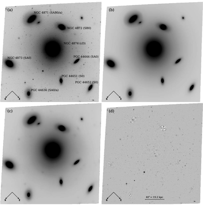
Figure 1.— Stacked HST ACS/WFC F814W image of the field roughly centered on NGC 4874. The size of the field is $3\farcm 52\times 3\farcm 56$. (a) The drizzled science image, shown at the observed orientation. Bright extended galaxies in the field are labeled and their morphological types from NED are shown in parentheses. (b) The sum of ELLIPSE-generated isophotal models for NGC 4874 and nine surrounding galaxies. (c) The sum of galaxy isophotal models and a large-scale residual map constructed using SExtractor. (d) The final “residual image” used for the object detection with the isophotal models and SExtractor background subtracted.

Figure 1 (a) shows our ACS/WFC F814W image of the NGC 4874 field, along with the designations and morphological classifications from the NASA/IPAC Extragalactic Database (NED) for eight bright galaxies (including NGC 4874 itself).

Table 1Observational Details of the Data Sets

Program	Dataset	Instrument/	Bandpass	Exp. Time	$m_{1}$	Magnitude
ID		Detector		(sec)	(mag)	Symbol
11711	JB2I01010	ACS/WFC	F475W	2394.0	26.056	$g_{475}$
10861	J9TY19040	ACS/WFC	F475W	2677.0	26.045	$g_{475}$
11711	JB2I01020	ACS/WFC	F814W	10425.0	25.947	$I_{814}$
11711	IB2I02040	WFC3/IR	F160W	10790.8	25.946	$H_{160}$

We also observed NGC 4874 with the Wide Field Camera 3 IR Channel (WFC3/IR) in parallel for six additional orbits of GO-11711, with four of the orbits in the longest wavelength F160W ($H_{160}$) bandpass, during primary ACS/WFC observations of the neighboring Coma giant elliptical NGC 4889. The WFC3/IR focal plane array consists of a single detector with a field of view of $2\farcm 27{\,\times\,}2\farcm 05$. The calibrated WFC3/IR $H_{160}$ exposures were retrieved from STScI/MAST and combined into a final geometrically corrected image using the MultiDrizzle (Koekemoer et al. 2003; Fruchter et al. 2009) task in the PyRAF/STSDAS package. As in Blakeslee et al. (2012), we used an output pixel scale of 0$\farcs$1 pix^-1, which is twice that of ACS/WFC. Table 1 summarizes the observational details of our imaging data; note that the two sets of F475W data from the two different programs were combined by Apsis into a single stacked image.

We corrected for Galactic extinction toward NGC 4874 assuming $E(B{-}V)=0.0091$ mag (Schlegel et al. 1998) and the revised ACS/WFC and WFC3/IR extinction coefficients (for $R_{V}{\,=\,}3.1$) from Schlafly & Finkbeiner (2011); the resulting corrections were small, amounting to 0.030, 0.014, and 0.005 mag in $g_{475}$, $I_{814}$, and $H_{160}$, respectively. When we derived K-corrections for 12 Gyr model spectral energy distributions, which are redshifted to the NGC 4874 distance (Benítez 2000), with $[{\rm Fe/H}]$ $=-1.7$ and $-0.7$ (Bruzual & Charlot 2003; C. Chung, private communication), corresponding to blue and red peak GCs, the average corrections are 0.05, 0.00, and $-0.02$ mag for $g_{475}$, $I_{814}$, and $H_{160}$, respectively. Since it is uncertain how good the evolutionary stellar population synthesis models are at NIR wavelengths and the estimated K-corrections are small but model-dependent, we have not applied them to our magnitudes and colors for GC candidates.

In this paper, we calibrate the ACS photometry to the AB system following Bohlin (2012) and adopting the time-variable zero points from the online ACS Zeropoints Calculator. The WFC3 photometry is calibrated using the AB zero points from the online WFC3 zero point tables (06 March 2012 revision). For reference, the adopted zero points are provided in Table 1; in the case of F475W, we used an exposure time-weighted average of the zero points for the two different observations.

3. Photometric Analysis

3.1. Galaxy and Background Subtraction

In order to detect point-like objects embedded in the extended galaxy halo light, we first removed the smooth galaxy light profiles from the final combined images. We constructed elliptical isophotal models for each of the bright galaxies in each of the stacked bandpass images using the IRAF/STSDAS tasks ELLIPSE and BMODEL, which use the fitting algorithm and the uncertainty estimation method described by Jedrzejewski (1987) and Busko (1996). We started by making an initial model (improved with later iterations) of the brightest galaxy (NGC 4874), then progressed by modeling the other galaxies in order of their luminosity. When running ELLIPSE, we first masked bright foreground stars, bad pixels, and any bright galaxies in the field except for the galaxy being fitted; then we modeled the isophotes of the galaxy light distribution. Using the isophotal parameters from ELLIPSE, we then build a smooth galaxy model with BMODEL. After subtracting the model from the original image, we fitted isophotes of the next brightest galaxy and subtracted this isophotal model as well. We repeated this process until we had subtracted ten galaxies in the ACS/WFC image and four galaxies (NGC 4874 itself and three surrounding galaxies) in the WFC3/IR image. As mentioned above, it was necessary to model the galaxies iteratively in order to achieve the cleanest model subtractions (e.g., Alamo-Martínez et al. 2013).

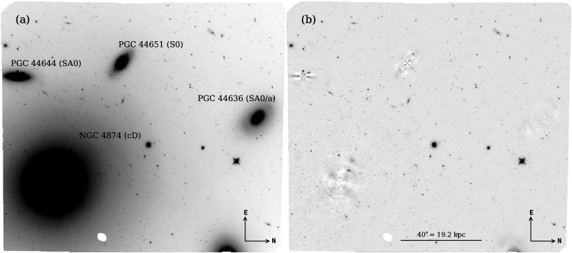
Figure 2.— Stacked HST WFC3/IR F160W observation of NGC 4874 and surrounding region. The field size is $2\farcm 36\times 2\farcm 09$; north is to the right and east is up. (a) The drizzled F160W science image; NGC 4874 and three neighboring galaxies are labeled. (b) The same image after subtracting our isophotal models of the four large galaxies and a SExtractor-generated background map.

After subtracting the elliptical isophotal models, we modeled the residual background using SExtractor (Bertin & Arnouts 1996) to fit a two-dimensional bicubic spline with the parameters ${\tt BACK\_SIZE}=32$ and ${\tt BACK\_FILTERSIZE}=3$. This removes residual structure on scales much larger than the full width half maximum (FWHM) of the point spread function (PSF), and thus does not detrimentally affect the point source photometry (see Jordán et al. 2004). We note that subtraction of the isophotal model generated by the BMODEL task sometimes results in a noticeable discontinuity in surface brightness at the “edge” of the model. However, because we modeled the galaxies to very low surface brightness levels, and performed careful iterative modeling to achieve flat local background levels, such residual “edge” features were generally in the noise. In addition, spurious detections associated with the model edges would be removed by our point source selection criteria described below. Panels (b) through (d) of Figure 1 respectively show our combined isophotal models for the galaxies labeled in panel (a) plus two additional galaxies; the isophotal galaxy models plus the residual background map; and the final “residual image” after subtracting the galaxy and residual background models. For comparison, the stacked WFC3/IR F160W science image and residual image following galaxy and background map subtraction are presented in Figure 2. Because of the smaller field of view, only NGC 4874 and the three other galaxies (labeled) were modeled. Disky residuals are noticeable in some cases, but the subtracted images are generally quite clean, revealing many faint sources.

3.2. Object Detection and GC Candidate Selection

Object detection and photometric measurements were performed on the final residual images using SExtractor independently for each bandpass (i.e., in “single-image mode”). For the ACS photometry, we used the RMS weight images produced by Apsis as the SExtractor weight images (type MAP_RMS). For the WFC3/IR F160W photometry, we used a variance map (type MAP_VAR) constructed from the inverse-variance image produced by MultiDrizzle, and including the photometric noise from the science data image itself. In order to flag bad pixels, we made maps denoting blank image areas, pixels close to frame boundaries, and the circular detector defect visible in WFC3/IR images. The maps were referenced using FLAG_IMAGE in SExtractor. We ran SExtractor with a Gaussian detection filter to identify objects with an area of at least four connected pixels with a flux level above two times the background rms in the ACS F475W and F814W images. The slightly larger value of ${\tt DETECT\_MINAREA}=5$ was used for the WFC3/IR F160W image since the subpixel resampling from the original pixel scale to 0$\farcs$1 pix^-1 during the MultiDrizzle run causes more noise correlation between neighboring pixels. Separation of blended objects was performed using the SExtractor parameter ${\tt DEBLEND\_NTHRESH}=32$ and ${\tt DEBLEND\_MINCONT}=0.005$ and $0.007$ for ACS/WFC and WFC3/IR images, respectively.

The source catalogs extracted from the ACS/WFC F475W and WFC3/IR F160W images were matched against the ACS/WFC F814W catalog using the source positions to remove spurious sources from the multi-band data. We estimate total $I_{814}$ magnitudes for each object using the MAG_AUTO values. For the color estimations, the aperture photometry was performed using apertures with radii of 3 pixels (0$\farcs$15 for ACS and 0$\farcs$30 for WFC3/IR data) as in Blakeslee et al. (2012). Aperture corrections were determined for a typical GC at the Coma distance using PSF-convolved King models. The empirical PSFs for ACS/F475W, ACS/F814W, and WFC3/F160W bands were produced with the same drizzle parameters, including interpolation kernel, pixfrac, and output scale (all of which have important effects for magnitudes measured within small apertures) as the science data for each band. Our final aperture corrections for the 3-pixel radius SExtractor apertures are $-0.24$, $-0.26$, and $-0.28$ mag for $g_{475}$, $I_{814}$, and $H_{160}$, respectively, with uncertainties of $0.01$ mag.

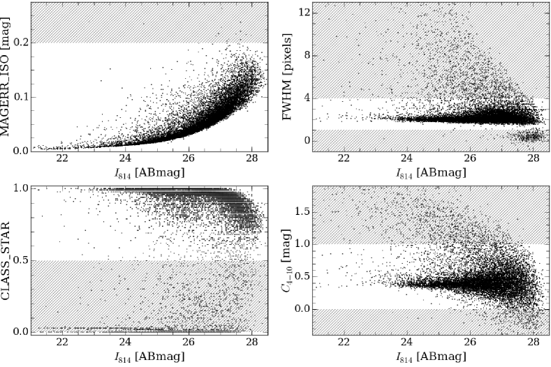
Figure 3.— Initial criteria for GC candidate selection as a function of $I_{814}$ MAG_AUTO (an estimate of the total magnitude) from SExtractor. Clockwise from top left panel: RMS error for the isophotal magnitude (scaling inversely with detection signal-to-noise), full width at half-maximum, magnitude difference between 4- and 10-pixel diameter apertures, and the CLASS_STAR stellarity index values are plotted against MAG_AUTO. The gray hatched regions mark the parameter ranges over which objects are excluded under each criterion (see Section 3.2 for details).

In order to identify GC candidates, we used the F814W photometric catalog because of its higher signal-to-noise ratio ($S/N$) than the F475W data, and larger field of view than the WFC3/IR image. Prior to classifying candidates as GCs, we required the SExtractor parameter ${\tt FLAGS}<4$ for all three bands in order to exclude sources too near the image edges (e.g., Puzia et al. 2014). To limit our analysis to sources detected with $S/N\,{>}\,5$, we require ${\tt MAGERR\_ISO}$ (the rms error on the magnitudes within the isophotal area) in F814W to be less than 0.2 mag. Figure 3 shows our photometric selection criteria for probable GCs as a function of the total $I_{814}$ magnitudes, for which we adopt the values of MAG_AUTO measured with SExtractor (as an additional sanity check, we require the uncertainty in MAG_AUTO to be less than 1 mag). As demonstrated in the top left panel of Figure 3, the uncertainties on the isophotal magnitudes are smaller than 0.1 mag for the majority of the GC candidates brighter than the turnover of the GC luminosity function (GCLF), which is expected to occur at an AB magnitude of $I_{814}\approx 26.9\pm 0.2$ mag at the distance of the Coma cluster (Peng et al. 2009, 2011).

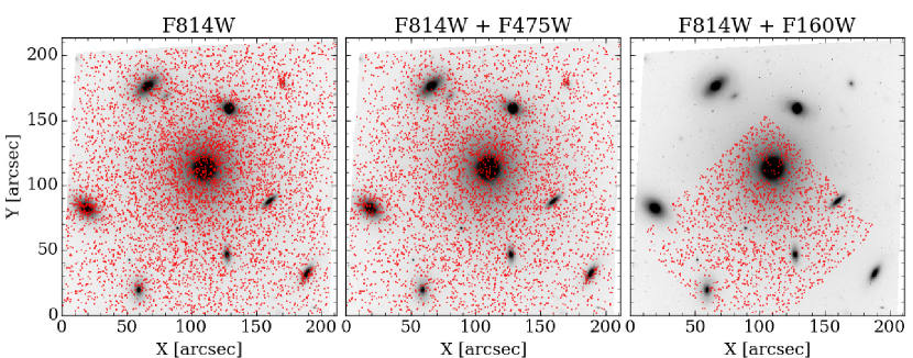
Figure 4.— Spatial distributions of GC candidates in the magnitude range of $21.5<I_{814}<27.0$ mag (red points) plotted on top of the ACS/WFC F814W image. The left panel shows positions of the GC candidates selected only from the F814W photometry. The middle panel shows GC candidates from the matched F814W and F475W photometric catalogs with colors $0.5<g_{475}{-}I_{814}<1.6$ mag and color errors $<0.2$ mag. The right panel shows the positions of the GC candidates from the matched F814W and WFC3/F160W photometric catalogs with colors $-0.5<I_{814}{-}H_{160}<1.5$ mag, and color errors $<0.2$ mag.

The majority of GCs can be treated as point sources in our HST images since the mean half-light radius of typical GCs in early-type galaxies, $r_{h}\approx 3$ pc (Jordán et al. 2005, 2009; Masters et al. 2010), corresponds to $\sim\,$0$\farcs$006 at 100 Mpc. We therefore required candidate GCs to be compact. The SExtractor “stellarity index” values CLASS_STAR for all detected objects in F814W are plotted against the total magnitudes in the bottom left panel of Figure 3. The objects with ${\tt CLASS\_STAR}>0.5$ were classified as point-like sources, and thus possible GCs in Coma. Since the CLASS_STAR parameter is unreliable for the fainter objects, we also adopted additional criteria, based on the measured FWHM and concentration index $C_{4-10}$, to select faint point-like sources. The $C_{4-10}$ concentration index was introduced by Peng et al. (2011) in order to select likely GC candidates in Coma; it is defined as the difference between magnitudes measured in apertures with diameters of 4 pix and 10 pix. These additional selection criteria are graphically indicated in the right panels of Figure 3, where it is clear that a large fraction of the detected sources follow tight loci around a FWHM of 2 pix and a $C_{4-10}$ value of 0.4 mag.

We can thus summarize our initial (i.e., from the ACS F814W band, prior to any color cuts) GC candidate selection criteria as follows: ${\tt MAGERR\_ISO}{\,<\,}0.2$, $1{\,<\,}{\tt FWHM}{\,<\,}4$ pix (with 0$\farcs$05 pix^-1), and $0.0<C_{4-10}<1.0$ mag. We adopted a relatively broad cut in $C_{4-10}$ in order to include GC candidates that are more extended than typical GCs. However, using the above combination of criteria ensures that we select robustly characterized compact sources as GC candidates. In Figure 4 (left panel), we plot the locations in the ACS F814W image of the 6303 GC candidates selected solely from the F814W photometric data with magnitudes in the range $21.5<I_{814}<27.0$ mag. These F814W GC candidates are widely distributed around the central cD galaxy NGC 4874, with localized concentrations around several of the surrounding cluster galaxies.

In this work, we also analyze the color properties of the GC candidates, and for this analysis we impose additional criteria to reject objects that are likely to be contaminants based on their color. In matching the F814W-selected candidates with the ACS F475W object catalog, we imposed a broad color cut of $0.5<g_{475}{-}I_{814}<1.6$ mag (e.g., Peng et al. 2011) for the GC candidates. We plot in the central panel of Figure 4 the 4612 GC candidates from the left panel that have colors within this range and color uncertainties less than 0.2 mag. In matching the F814W candidates to the WFC3/F160W catalog, we restricted the colors to $-0.5<I_{814}{-}H_{160}<1.5$ mag (e.g., Blakeslee et al. 2012); again requiring color uncertainties less than 0.2 mag, we plot the 1719 GC candidates within this $I_{814}{-}H_{160}$ color interval in the right panel of Figure 4. Note that the paucity of matched F814W+F160W GC candidates near the galaxy NGC 4873 (labeled in Figure 1) occurs because this galaxy is off the edge of the WFC3/IR field of view (see Figure 2) and was not cleanly subtracted by isophotal modeling; thus, we did not obtain reliable F160W photometry for objects in its immediate vicinity.

3.3. Comparison with ACS Coma Cluster Survey

Photometry in the ACS $g_{475}$ and $I_{814}$ bands for GCs in the region around NGC 4874 was previously published by Peng et al. (2011) using data from HST program GO-10861, ACSCCS. Our exposure time in F814W is 7.4 times longer than that obtained by the ACSCCS, implying a $S/N$ about 2.7 times greater, or a limiting magnitude more than 1 mag deeper in this band. For F475W, because we incorporated the ACSCCS exposures into our stacked image, our exposure time is nearly a factor of two longer ($\sim 40$% higher $S/N$) than for the ACSCCS data alone (the images did not overlap completely because they were taken at different orientations). Since the addition of the ACSCCS F814W data would have increased our $S/N$ by $\lesssim 7\%$, we opted not to include those data in our stacked image in that bandpass. Peng et al. (2011) performed source photometry on the galaxy-subtracted ACSCCS images using SExtractor with 3 pixel radius apertures and then selected GC candidates based on color and source concentration; thus, the analysis was quite similar to our own and can be used as a straightforward check on our photometry.

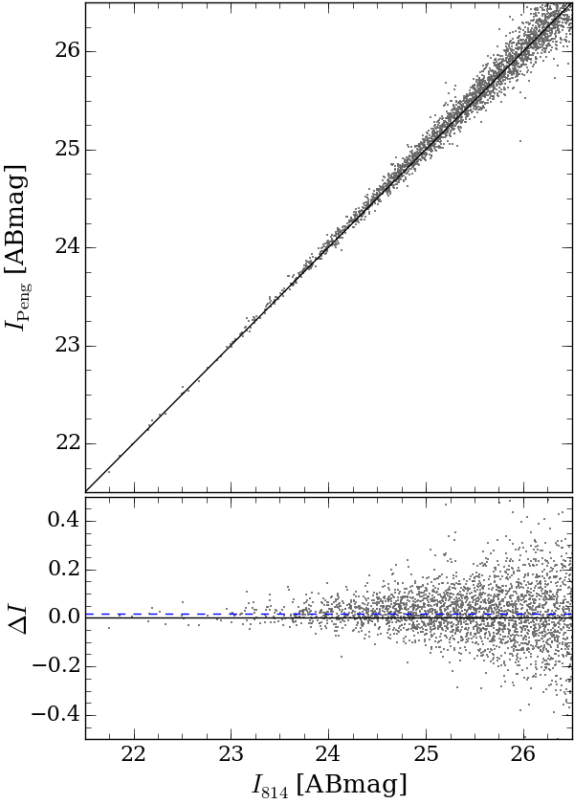
Figure 5.— Comparison of 3-pixel radius aperture magnitudes in the ACS F814W passband from the photometry of Peng et al. (2011), denoted by $I_{\rm Peng}$, with those from our photometry. The points are objects in common for the two data sets. The black solid line in the upper panel represents equality, and is not a fit. In the lower panel, the magnitude differences $\Delta{I}=I_{\rm Peng}-I_{814}$ are plotted as a function of our $I_{814}$ magnitude. The black solid line shows a zero magnitude difference, while the blue dashed line indicates the median offset in $\Delta{I}$ of 0.017 mag.

Figure 5 shows a comparison of $I_{814}$ magnitudes from Peng et al. (2011) with those of the present study; for consistency, we compare the magnitudes without correction for Galactic extinction. The data for this comparison (unlike the case for $g_{475}$) are fully independent. The top panel of the figure shows that the overall agreement is very good over a range of 5 mag; the slope of the residuals over this magnitude range is consistent with zero. Peng et al. cut their GC selection at $I_{814}=26.5$ mag, in part because the photometric error in their $C_{4-10}$ concentration parameter became too large to distinguish point sources and background galaxies at about this magnitude; as expected from the increased depth, our F814W data are able to distinguish point sources from extended objects to about 1 mag fainter (compare their Figure 2 with our Figure 3).

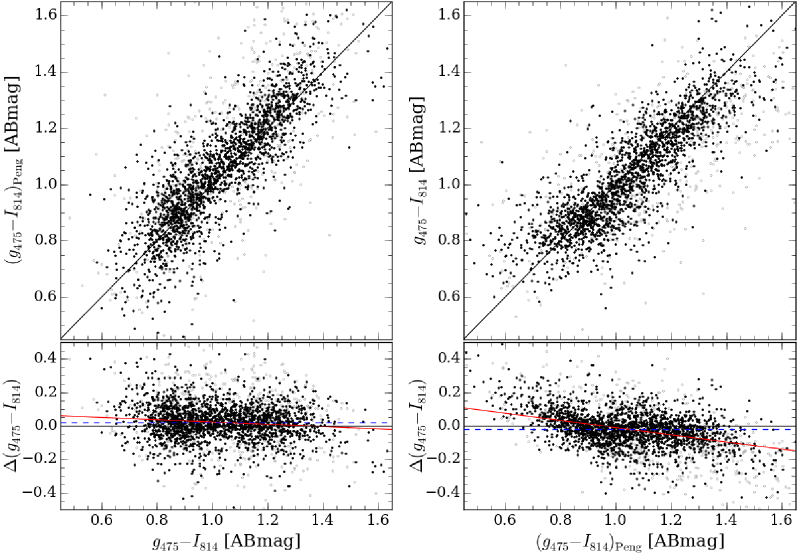
Figure 6.— Comparison between our $g_{475}{-}I_{814}$ color values and those from the photometry of Peng et al. (2011), denoted by $({g_{475}{-}I_{814}})_{\rm Peng}$. Black points have color errors in the Peng et al. photometry smaller than 0.2 mag. The objects with larger color uncertainties are marked by gray points. The black solid lines in the upper panels represent the one-to-one relation. The lower panels show the differences in the colors between these two data sets. In each lower panel, the zero and median difference values are marked by the black solid line and the blue dashed line, respectively. The red solid lines show the robust linear relations given in the text.

The lower panel of Figure 5 shows the residuals $\Delta{I}=I_{\rm Peng}{\,-\,}I_{814}$ for 2673 point sources (selected based on our measurements) in common between the two data sets down to $I_{814}=26.5$ mag (again, from our measurement). The mean offset in $I_{814}$ is $0.014\pm 0.002$ mag, with a scatter of 0.105 mag, and the median offset is 0.017 mag, in the sense that the ACSCCS magnitudes are slightly fainter. If we limit the range to $21.5<I_{814}<25.5$ mag, then the number of sources is reduced by approximately half to 1308, with both a mean and median offset of 0.022 mag, and a scatter of 0.063 mag. Peng et al. (2011) calibrated their photometry using the AB zero points from Sirianni et al. (2005); however, adopting the calibration from the online ACS zero point calculator for the appropriate date of the observations would decrease the size of the offset by only 0.002 mag. Given the uncertainty in the time-dependence of the zero point (Bohlin 2012), the lack of CTE correction for the ACSCCS data, the difference in the drizzle parameter settings (e.g., linear versus lanczos3 interpolation kernels), the possibility of small focus variations (e.g., Jee et al. 2007), and the much greater depth of our F814W observations (which could result in subtle differences in the SExtractor photometry), we consider the systematic offset of $\lesssim 0.02$ mag to be reasonable. The scatter in the residuals (dominated by the much shallower ACSCCS measurements) increases as expected at fainter magnitudes, but there is no evidence for a systematic trend in the residuals with magnitude.

Figure 6 compares the $g_{475}{-}I_{814}$ colors for point sources in common between Peng et al. (2011) and the present study over a range in $I_{814}$ from 21.5 to 26.5 mag. The left and right panels show, respectively, the comparison as a function of our and the ACSCCS color measurements. In both panels, the black points represent sources in Peng et al. (2011) with estimated color errors $<0.2$ mag, while the gray points show sources with color errors larger than 0.2 mag. Considering all the points, black and gray, over the plotted color range of $0.45<g_{475}{-}I_{814}<1.65$ mag, the median offset is 0.026 mag, the rms scatter is 0.13 mag, and the biweight scatter (more robust against outliers) is 0.12 mag. Considering just the black points, the median offset is 0.020 mag, the rms scatter is 0.11 mag, and the biweight scatter is 0.10 mag. The sense of the offset is that the ACSCCS $g_{475}{-}I_{814}$ colors are slightly redder than ours; if we were to recalibrate the Peng et al. photometry using the online ACS Zeropoints Calculator, the ACSCCS colors would become bluer by 0.021 mag, reducing the median color offset for the black points to 0.001 mag. However, because of observational error, the observed offset also has a dependence on color.

The lower panels of Figure 6 show the color differences $\Delta{(g_{475}{-}I_{814})}$ (defined as $y$-axis color minus $x$-axis color) plotted as a function of both our colors and the ACSCCS colors, which we label $(g_{475}{-}I_{814})_{\rm Peng}$. The solid red lines show robust linear regressions for the black points in these panels; the slopes of the $\Delta{(g_{475}{-}I_{814})}$ regression lines are $-0.068\pm 0.012$ and $-0.214\pm 0.010$ when fitted versus our $g_{475}{-}I_{814}$ colors and versus $(g_{475}{-}I_{814})_{\rm Peng}$, respectively. Thus, the slope is more than a factor of three steeper when fitted as a function of the ACSCCS colors. This is understandable in light of the larger measurement errors for those colors. Since the vast majority of these objects are GCs, which intrinsically define a fairly narrow color range $0.7\lesssim g_{475}{-}I_{814}\lesssim 1.4$ mag, the scattering of the colors outside this color range primarily results from photometric errors, which are larger for the shallower ACSCCS measurements; thus, this error-induced slope is larger when plotted as a function of the ACSCCS colors. We find that we can reproduce the slopes and scatters in Figure 6 if we assume Gaussian errors with $\sigma=0.055$ mag for our color measurements and $\sigma=0.107$ mag the ACSCCS colors. For comparison, the median estimated color errors in the two catalogs are 0.063 mag and 0.098 mag, respectively. This suggests that our quoted errors may be slightly overestimated and the ACSCCS color errors slightly underestimated, but only by about 10% in each case.

We conclude that our measurements agree well with the ACSCCS photometry from Peng et al. (2011). The much greater exposure time of our $I_{814}$ imaging allows us to reach about 1 mag fainter in this bandpass, while our $g_{475}{-}I_{814}$ color errors for GC candidates are approximately a factor of two smaller than for the ACSCCS data. Systematic offsets in photometry are $\lesssim 0.02$ mag. In addition, our program adds deep $H_{160}$ photometry over the area of WFC3/IR field, which was not available for the earlier study.

4. Discussion

4.1. Color-Magnitude Diagrams and “Tilts”

As discussed in the Introduction, GC systems of massive galaxies generally follow bimodal distributions in optical color. However, the peaks in the color distribution can vary with the magnitude range of the GCs considered. For instance, Ostrov et al. (1998) and Dirsch et al. (2003) found that for GCs more than 2 mag brighter than the turnover of the GCLF in the galaxy NGC 1399, the blue and red peaks merged together into a single broad distribution. More generally, the mean color of the blue GCs tends to get redder at brighter magnitudes (Harris et al. 2006; Mieske et al. 2006, 2010; Strader et al. 2006; Harris 2009), possibly indicating an increasing mean metallicity with GC luminosity. This effect, known alternately as the GC color-magnitude relation, mass-metallicity relation, or informally as “the blue tilt” (a “tilt” of the blue peak towards a redder mean color at bright magnitudes) is most generally believed to be a consequence of self-enrichment within the most massive GCs (e.g., Bailin & Harris 2009).

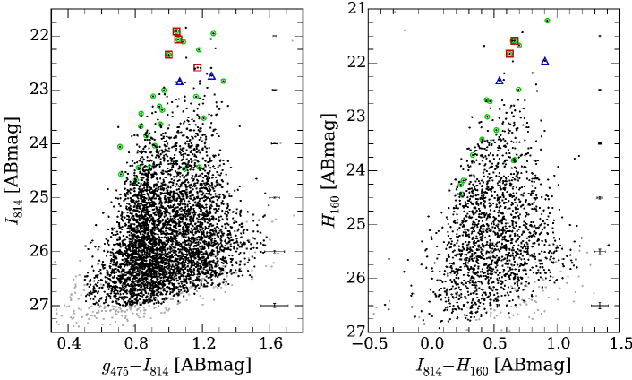
Figure 7.— The optical color-magnitude diagram for GC candidates in the NGC 4874 field from ACS/WFC F475W and F814W imaging data (left) and the optical-NIR color-magnitude diagram for GC candidates from ACS/WFC F814W and WFC3/IR F160W imaging data (right). The final GC samples from Figure 4 are plotted in black; the gray points were excluded from further analysis. Error bars (near the right edge of each panel) represent the mean errors of the magnitudes and colors in a magnitude bin. Red squares show ultra-compact dwarf galaxies (UCDs, classified purely on the basis of luminosity and color) spectroscopically confirmed as members of the Coma cluster, while blue triangles indicate likely UCDs with uncertain redshifts (Chiboucas et al. 2011). Green circles mark photometrically classified UCDs or “dwarf-globular transition objects” from Madrid et al. (2010). These objects all have photometric properties consistent with being extensions of the GC population, and we do not attempt to exclude them from our analysis.

Figure 7 displays the color-magnitude diagrams (CMDs) for GC candidates in NGC 4874 in both the optical $g_{475}{-}I_{814}$ (left panel) and optical-NIR $I_{814}{-}H_{160}$ (right panel) colors. We have marked in these panels the objects, included in our GC selection, that are spectroscopically confirmed (red squares) or possible (blue triangles) ultra-compact dwarfs (UCDs) from the study of Chiboucas et al. (2011). In this case, UCDs are defined simply as compact stellar systems with colors similar to GCs and absolute $R$ magnitude $M_{R}{\,<\,}-11$ mag. Because of the larger ACS/WFC field, there are six of these objects in the optical CMD of the left panel, but four in the right panel (in both cases, two of the UCDs are uncertain Coma members based on their spectra). We also indicate objects (green circles) that were selected by Madrid et al. (2010) based on ACSCCS imaging as candidate (lacking spectroscopic confirmation) UCDs or “dwarf-globular transition objects,” defined as objects having GC-like colors and half-light radii in the range of 10 to 100 pc (if located at the distance of the Coma cluster). Although there are more objects in the left panel, and the ridge-line of the blue GC component is also much more distinct in the $g_{475}{-}I_{814}$ color, overall the CMDs appear fairly similar over a range of 5 mag in luminosity, with an overall tilt towards redder colors at the brightest magnitudes where objects tend to be classified as UCDs.

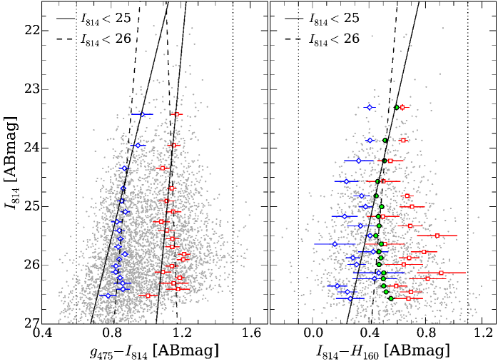
Figure 8.— $I_{814}$ vs. $g_{475}{-}I_{814}$ color-magnitude diagram (left) and $I_{814}$ vs. $I_{814}{-}H_{160}$ color-magnitude diagram (right). The black points in Figure 7 are plotted in gray in these diagrams for clarity. We subdivided each CMD into eighteen magnitude bins, each with a fixed number of data points, except the brightest two bins in each panel, for which the number is half that of the other bins. In the left panel, the positions of the first and second peaks (mean positions) in the GMM double Gaussian model for each magnitude bin are plotted with blue open diamonds and red open squares, respectively. The error bars represent the uncertainties on each peak calculated from the non-parametric bootstrap resampling by the GMM algorithm. In the right panel, the green circles with error bars indicate the positions of the average peaks for each magnitude bin. We also plot the positions of the double peaks from the GMM fits, which are marked by blue open diamonds and red open squares, along with the error bars from the GMM bootstrap resampling. The thick solid and dashed lines indicate the linear fits to the peak positions when the faintest magnitudes used in the each fit are $M_{814}=-10.0$ mag and $-9.0$ mag, respectively. For the fits, we adopted the blue and red color limits marked by the vertical dotted lines.

In order to quantify the degree of “blue tilt” in NGC 4874, we binned the GC candidates by magnitude and applied the Gaussian Mixture Modeling (GMM) code of Muratov & Gnedin (2010) to each bin. Figure 8 shows CMDs similar to the previous figure, but now using $I_{814}$ for the magnitude in both cases, and showing the locations of the color peaks from the bimodal GMM decompositions for eighteen bins in magnitude down to $I_{814}\approx 26.5$ mag. Because the GMM algorithm can be sensitive to objects that are scattered into the tails of the distribution by observational errors (which increase at fainter magnitudes), we have restricted these magnitude-grouped samples to the color ranges $0.6<g_{475}{-}I_{814}<1.5$ mag and $-0.1<I_{814}{-}H_{160}<1.1$ mag, indicated by the dotted lines in Figure 8. For the $I_{814}$ versus $g_{475}{-}I_{814}$ CMD (left panel), each bin has 240 GCs, while for the $I_{814}{-}H_{160}$ CMD (right panel), each bin has 90 GCs; the exceptions are the brightest two bins in each panel, which have only half the number of GCs as the other bins. In the left panel of Figure 8, there is clear evidence for a “blue tilt,” as well as some suggestion of a “red tilt” for the peak positions at magnitudes $I_{814}<25$ mag, corresponding to absolute $M_{814}<-10$ mag. Linear fits to the red and blue peak positions for bins brighter than this magnitude are shown by the solid black lines, defined by the following relations:

$$(g_{475}{-}I_{814})_{\rm blue} = (0.88\pm 0.01)\,-\,(0.082\pm 0.020)$$

$${\times}(I_{814}-24.5),\;M_{814}<-10.0\,;$$ (1)

$$(g_{475}{-}I_{814})_{\rm red} = (1.14\pm 0.01)\,-\,(0.031\pm 0.023)$$

$${\times}(I_{814}-24.5),\;M_{814}<-10.0\,.$$ (2)

The error bars here reflect the statistical uncertainties in the parameters from the linear fits.

The slope $\gamma_{814,{\rm blue}}\equiv{d(g_{475}{-}I_{814})}/{dI_{814}}=-0.082$ of the blue tilt is highly significant (4-sigma) and is among the steepest observed to date. For comparison, Mieske et al. (2006, 2010) found $\gamma_{850,{\rm blue}}\equiv{d(g_{475}{-}z_{850})}/{dz_{850}}=-0.042\pm 0.015$ for M87 in Virgo and $\gamma_{850,{\rm blue}}=-0.088\pm 0.025$ for NGC 1399 in Fornax, the central giant ellipticals in each cluster. Using the observed relationship for GCs in NGC 1399, $g_{475}{-}I_{814}=0.13+0.75(g_{475}{-}z_{850})$ from Blakeslee et al. (2012), this would imply $\gamma_{814,{\rm blue}}=-0.032$ and $-0.065$ for M87 and NGC 1399, respectively. Further, NGC 4472 (M49), the brightest galaxy in Virgo, has no significant blue tilt at all; thus, the color-magnitude trend in NGC 4874 is exceptionally steep compared to the Virgo and Fornax clusters. This may be related to an abundance of UCDs in the dense core of the Coma cluster. It is clear that the tilt becomes greater for objects at $I_{814}<23.5$ mag ($M_{814}<-11.5$ mag), where the sample may be dominated by UCDs, which tend to have colors intermediate between the blue and red peaks of the optical GC color distribution (e.g., Liu et al. 2015). It is likely that UCDs represent a mix of stripped galactic nuclei and luminous GCs; as already indicated in Figure 7, we have not attempted to exclude UCDs from our sample if they satisfy our selection criteria.

The derived color-magnitude slope becomes markedly less steep when the fit is extended to fainter GCs. The dashed lines in Figure 8 indicate the following linear fits to the peaks with $I_{814}<26$ mag ($M_{814}<-9$ mag):

$$(g_{475}{-}I_{814})_{\rm blue} = (0.88\pm 0.01)\,-\,(0.027\pm 0.010)$$

$${\times}(I_{814}-24.5),\;M_{814}<-9.0\,;$$ (3)

$$(g_{475}{-}I_{814})_{\rm red} = (1.15\pm 0.01)\,+\,(0.012\pm 0.015)$$

$${\times}(I_{814}-24.5),\;M_{814}<-9.0\,.$$ (4)

Thus, when the fit is extended by one magnitude, the slope of the color-magnitude trend for blue peak positions is reduced by a factor of three. The shallower slope over the wider magnitude range reflects the nonlinearity of the color-magnitude tilt (e.g., Harris 2009; Mieske et al. 2010), which may result from a minimum mass threshold for self-enrichment. For the red GC peak, the fitted slope over this broader magnitude range is essentially zero.

We can estimate the scaling of metallicity $Z$ with the GC luminosity $L$ in the $I_{814}$ bandpass using the empirical broken-linear calibration from Peng et al. (2006) for the metallicity as a function of $g_{475}{-}z_{850}$ color. Since the “tilt” occurs for the blue GC population, we use the linear relation appropriate for the blue GCs: $[{\rm Fe/H}]=-6.21-(5.14\pm 0.67)(g_{475}{-}z_{850})$. This is the same relation used by Mieske et al. (2010) for deriving the mass-metallicity scaling from their blue tilt measurements in the ACS Virgo and Fornax Cluster Survey data (Côté et al. 2004; Jordán et al. 2007). Coupled with the above relation between $g_{475}{-}I_{814}$ and $g_{475}{-}z_{850}$, and our measurement of $\gamma_{814,{\rm blue}}=-0.082\pm 0.020$ for $M_{814}<-10$ mag, we find $Z\propto L^{1.4\pm 0.4}$ at these highest luminosities, or if we assume a constant mass-to-light ratio for blue-peak GCs as in Mieske et al., then $Z\propto M_{\rm GC}^{1.4\pm 0.4}$ for the scaling with GC mass. Of course, if we use the slope $\gamma_{814,{\rm blue}}=-0.027\pm 0.010$ from the linear fit extending to $M_{814}=-9$ mag, then the mean mass-metallicity scaling over this magnitude range becomes $Z\propto M_{\rm GC}^{0.5\pm 0.2}$, again reflecting the nonlinearity of the relation.

For the $I_{814}$ versus $I_{814}{-}H_{160}$ CMD (Figure 8, right panel), we find no significant evidence for a “tilt” in the colors of either the red or blue peaks from the GMM bimodal decompositions within the magnitude bins. This may be because of the poorer statistics and/or weaker separation of blue and red GCs for this optical-NIR color. Notably, however, we do find a significant trend for the overall mean GC color (based on the unimodal GMM fit) to become redder for the brighter magnitude bins. The solid line in this panel is a fit to the $I_{814}{-}H_{160}$ unimodal peak positions for bins with $M_{814}<-10$ mag; the dashed line again extends the fit one magnitude fainter than this and is significantly less steep. The fits are given by the following relations:

$$(I_{814}{-}H_{160})_{\rm mean} = (0.47\pm 0.01)\,-\,\,(0.093\pm 0.013)$$

$${\times}(I_{814}-24.5),\;M_{814}<-10.0\,;$$ (5)

$$(I_{814}{-}H_{160})_{\rm mean} = (0.50\pm 0.01)\,-\,\,(0.034\pm 0.010)$$

$${\times}(I_{814}-24.5),\;M_{814}<-9.0\,.$$ (6)

The slope of this “mean tilt” in $I_{814}{-}H_{160}$ for $M_{814}<-10$, $I_{814}<-25$ mag, is highly significant. The color sequence appears nearly vertical at magnitudes fainter than this, although the slope of the fit for $M_{814}<-9$ mag (dashed line) remains significant because of the brightest bins with their increasingly steep slope. Although the relation between $I_{814}{-}H_{160}$ and metallicity has not been empirically calibrated for extragalactic GC systems, we can check for consistency by using the linear version of the relation between $I_{814}{-}H_{160}$ and $g_{475}{-}I_{814}$ derived in Sec. 4.3 below, which has a slope $d(I_{814}{-}H_{160})/d(g_{475}{-}I_{814})=1.13\pm 0.04$. Combining this with the same set of relations between $g_{475}{-}I_{814}$, $g_{475}{-}z_{850}$, and $[{\rm Fe/H}]$ as above (although the adopted $[{\rm Fe/H}]$ transformation is only strictly applicable for blue GCs), we can derive the mass-metallicity scaling from the fitted slopes ${d(I_{814}{-}H_{160})}/{dI_{814}}$ in Eqs. (5) and (6). For $M_{814}<-10$ mag, the result is again $Z\propto M_{\rm GC}^{1.4}$, and the exponent again drops to $\sim 0.5$ if we use the $I_{814}{-}H_{160}$ fit extending to $M_{814}=-9$ mag.

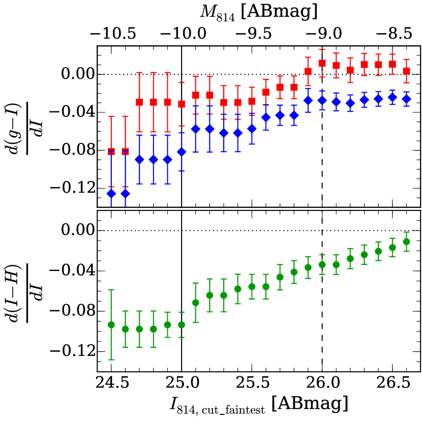
Figure 9.— Fitted slopes as a function of the faintest magnitude cut in the ACS F814W passband. The red squares and blue diamonds in the top panel are the slope values of the linear fits to the red and blue peak positions, respectively, in the $g_{475}{-}I_{814}$ versus $I_{814}$ CMD shown in Figure 8 for varying limiting magnitudes of the fit. The green points in the bottom panel are the slopes of the linear fits to the overall mean positions in the $I_{814}{-}H_{160}$ versus $I_{814}$ CMD in Figure 8 for varying limiting magnitudes of the fit. The vertical solid and dashed lines indicate the limiting magnitude values for the corresponding linear fits shown in Figure 8. The trends seen here towards shallower slopes with fainter limiting magnitudes indicate that the relations between mean color and magnitude are nonlinear, with the color peak positions in the CMDs becoming more vertical at fainter magnitudes; put another way, the “tilts” are only significant for the brightest GCs.

The equality in the exponents of the mass-metallicity relations derived from $g_{475}{-}I_{814}$ and $I_{814}{-}H_{160}$ may seem strange, given that in former case it is based on the trend in the blue GC component with magnitude, while for the latter it is based on the overall mean $I_{814}{-}H_{160}$ trend with magnitude. In fact, it is somewhat fortuitous. The ratio of the slope for the mean $I_{814}{-}H_{160}$ in Eq. (5) to the slope for the blue peak in Eq. (1) is $1.13\pm 0.28$; the corresponding ratio for Eqs. (6) and (3) is $1.26\pm 0.42$. Both of these are in statistical agreement with the color-color slope found below in Sec. 4.3. This agreement can be understood, at least in part, from the fact that at progressively brighter magnitudes, the proportion of red-peak to blue-peak GCs increases in the $g_{475}{-}I_{814}$ histogram, as shown in Sec. 4.2 below. Thus, the overall mean slope of $g_{475}{-}I_{814}$ versus $I_{814}$ will be steeper than the average of the red and blue slopes. For completeness, we also fitted the overall mean $g_{475}{-}I_{814}$ color-magnitude relations, finding:

$$(g_{475}{-}I_{814})_{\rm mean} = (1.02\pm 0.01)\,-\,\,(0.060\pm 0.014)$$

$${\times}(I_{814}-24.5),\;M_{814}<-10.0\,;$$ (7)

$$(g_{475}{-}I_{814})_{\rm mean} = (1.03\pm 0.01)\,-\,\,(0.027\pm 0.008)$$

$${\times}(I_{814}-24.5),\;M_{814}<-9.0\,.$$ (8)

In both cases, the slope is steeper than the average of the red and blue slopes derived for the equivalent magnitude limits. In fact, the slope we find for the mean trend in Eq. (8) is the same as that for the blue tilt in Eq. (3). However, the conversion of these mean trends to a mass-metallicity scaling relation is less straightforward because there is a change in the slope of the color-metallicity relation at intermediate colors (e.g., Peng et al. 2006; Usher et al. 2012).

Figure 9 explores in more detail the dependence of the slope of the color-magnitude tilts as a function of the faint limit of the linear fits. The slope of the blue peak in $g_{475}{-}I_{814}$ remains significant regardless of the magnitude limit, while the slope for the red peak appears significant at the $2\sigma$ level only when the brightest two or three bins are considered, those with $M_{814}<-10.3$ mag. For $I_{814}{-}H_{160}$ (lower panel), although the separation into blue and red peaks is weak (as quantified in the following section), for bins with $M_{814}<-8.8$ mag, the slope of the overall trend towards a redder mean color (and thus metallicity) at brighter magnitudes is quite significant. However, the magnitude of the slope decreases continuously from $M_{814}\approx-10$ to $M_{814}\approx-8.5$ mag, again illustrating the nonlinearity of the trend.

4.2. Color Distributions

Figure 10.— Histograms of $g_{475}{-}I_{814}$ colors for GC candidates in the left panels of Figures 7 and 8 over different I-band magnitude ranges. The smooth Gaussian kernel density estimates are overplotted by thick solid curves. The hatched histogram is for UCDs (both confirmed cluster members and uncertain ones) from Chiboucas et al. (2011).

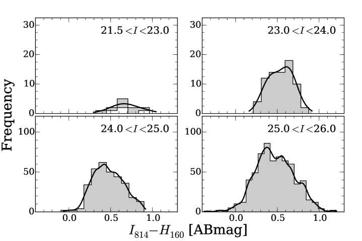
Figure 11.— Same as Figure 10 but for $I_{814}{-}H_{160}$ colors for GC candidates in the right panels of Figures 7 and 8.

As discussed in the previous section, the NGC 4874 GC candidates exhibit a distinct color-magnitude relation, at least at $I_{814}<25$ mag. Consequently, their color distributions should vary as a function of luminosity. Figure 10 plots the $g_{475}{-}I_{814}$ optical color histograms for the GC candidates in four different bins in $I_{814}$ magnitude; the distributions differ markedly from each other. In the brightest bin, consisting of objects at least 4 mag brighter than the expected turnover of the GCLF, the distribution is relatively red and broad, with no evidence for bimodality. The spectroscopic sample of UCDs from Chiboucas et al. (2011) is weighted towards the blue side of this distribution, but the sample is small and incomplete (see Figure 7), and selection effects could play a role. In the second bin, $23.0<I_{814}<24.0$ mag, there is clear bimodality in $g_{475}{-}I_{814}$, with the red peak being dominant. For $24.0<I_{814}<25.0$ mag, the blue peak becomes dominant, and this is true to an even greater extent for the faintest magnitude bin of $25.0<I_{814}<26.0$ mag.

Figure 11 shows the corresponding histograms of $I_{814}{-}H_{160}$ color using the same magnitude bins as in Figure 10. The samples are smaller because of the smaller field of WFC3/IR, but again we find that the color distribution appears broad, unimodal, and red for the brightest magnitude bin. Although any bimodality is much less evident than in $g_{475}{-}I_{814}$, the $I_{814}{-}H_{160}$ histogram for the $23.0<I_{814}<24.0$ mag range is skewed towards the red, while the histograms for the faintest two plotted magnitude ranges become progressively more skewed towards the blue. This is qualitatively similar to what is observed for $g_{475}{-}I_{814}$, and it is consistent with the striking “mean tilt” in the $I_{814}{-}H_{160}$ versus $I_{814}$ color-magnitude relation (Figure 8), for which the colors become bluer in $I_{814}{-}H_{160}$ at fainter magnitudes.

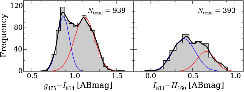
Figure 12.— Histograms of $g_{475}{-}I_{814}$ and $I_{814}{-}H_{160}$ colors for GC candidates within the magnitude range of $23.0<I_{814}<25.0$ mag. The black thick solid curve is the nonparametric density estimate constructed with a Gaussian kernel. We also plot the GMM double Gaussian model components for the heteroscedastic case with blue and red solid curves. The corresponding GMM analysis results are provided in Table 2.

In order to quantify the visual impressions given by Figures 10 and 11, we ran the GMM code on the $g_{475}{-}I_{814}$ and $I_{814}{-}H_{160}$ color distributions of the GC candidates in the various magnitude ranges shown in those figures. Table 2 summarizes the results of these GMM analysis runs, as well as the results for the broader magnitude range of $23.0<I_{814}<25.0$ mag, for which the $g_{475}{-}I_{814}$ and $I_{814}{-}H_{160}$ histograms are displayed in Figure 12. The bimodality in $g_{475}{-}I_{814}$ is significant for all the magnitude ranges explored in Table 2 except for the brightest; all the other bins have $p(\chi^{2})<0.01$, indicating less than 1% probability of the color data being drawn from a single Gaussian model, rather than the best-fit double Gaussian model with the tabulated means $\mu_{1},\mu_{2}$ and dispersions $\sigma_{1},\sigma_{2}$ and with the fraction of objects in the second (red) Gaussian given by $f_{2}$. The evidence for bimodality is stronger if the tabulated $D$, the separation between the Gaussians in units of the quadrature sum of their dispersions, is significantly $>2$, and if the kurtosis of the distribution $\hbox{\it kurt}<0$ (see Muratov & Gnedin 2010 and Blakeslee et al. 2012). The optical bimodality is especially pronounced, and the double Gaussian model parameters best constrained, within the $23.0<I_{814}<25.0$ mag range.

Figure 13.— Same as Figure 12 but for the cross-matched subsample of GC candidates with both ACS/WFC F475W and WFC3/IR F160W data. The GMM analysis results are in Table 3.

For the $I_{814}{-}H_{160}$ color index, the bimodality is only significant at the $>2\sigma$ level, $p(\chi^{2})<0.05$, for the $23.0<I_{814}<25.0$ mag range. Interestingly, however, for this magnitude range, the GMM code gives $f_{2}=0.624\pm 0.055$ for $g_{475}{-}I_{814}$, but $f_{2}=0.330\pm 0.144$ for $I_{814}{-}H_{160}$. Thus, although the bimodality is significant in this magnitude range for both $g_{475}{-}I_{814}$ and $I_{814}{-}H_{160}$, the preferred ratios of red/blue GCs differ at the $\sim 2\sigma$ level. This is similar to the result for NGC 1399, the cD galaxy in the Fornax cluster, for which Blakeslee et al. (2012) found significantly different bimodalities in $g_{475}{-}I_{814}$ and $I_{814}{-}H_{160}$, resulting from the nonlinear relation between these two color indices. However, it should be noted that although the magnitude range is the same, the $g_{475}{-}I_{814}$ sample has 939 objects while the $I_{814}{-}H_{160}$ sample has only 393 objects because the WFC3/IR field of view is smaller; it is not clear if the difference in color bimodalities is significant or not because the samples are different.

Figure 13 shows the histograms for the cross-matched subsample of 392 GC candidates in the $23.0<I_{814}<25.0$ mag range having both $g_{475}{-}I_{814}$ and $I_{814}{-}H_{160}$ colors. (There was one object in the sample of GC candidates with $I_{814}{-}H_{160}$ colors that was not included in the sample with $g_{475}{-}I_{814}$ colors.) The optical $g_{475}{-}I_{814}$ color is clearly bimodal, while the separation remains less clear for $I_{814}{-}H_{160}$. Table 3 presents the GMM analysis results for the $g_{475}{-}I_{814}$ and $I_{814}{-}H_{160}$ distributions of this homogeneous cross-matched sample. We include both the homoscedastic (common dispersion, $\sigma_{1}=\sigma_{2}$) and heteroscedastic ($\sigma_{1}\neq\sigma_{2}$) cases. For the heteroscedastic case, the preferred bimodal decompositions again differ significantly, with $f_{2}=0.604\pm 0.083$ and $f_{2}=0.324\pm 0.128$ for $g_{475}{-}I_{814}$ and $I_{814}{-}H_{160}$, respectively. On the other hand, for the homoscedastic case, the GMM code finds $f_{2}=0.493\pm 0.031$ and $f_{2}=0.436\pm 0.054$ for $g_{475}{-}I_{814}$ and $I_{814}{-}H_{160}$, respectively. Thus, if the color dispersion for the blue and red GC components are forced to be the same, then the bimodal decompositions for $g_{475}{-}I_{814}$ and $I_{814}{-}H_{160}$ are consistent. However, the heteroscedastic GMM results imply that the dispersions differ significantly, at least for the purely optical $g_{475}{-}I_{814}$ color, with the blue peak being significantly narrower; the same result has been found for other massive galaxies (e.g., Peng et al. 2006, 2009; Harris et al. 2016).

The heteroscedastic GMM results for $I_{814}{-}H_{160}$ in Tables 2 and 3 indicate that the color dispersion is slightly larger for the blue component than for the red component, the opposite of what we find for $g_{475}{-}I_{814}$. Exploring this issue in more detail, we found that the dispersion of the blue component in $I_{814}{-}H_{160}$, as well as the blue:red ratio, was sensitive to the presence of a small number of GC candidates with the bluest $I_{814}{-}H_{160}$ colors. Table 4 reports the results for heteroscedastic GMM tests when the two and four bluest GCs in $I_{814}{-}H_{160}$ are removed from the sample. For instance, when the blue limit is changed by $+0.15$ mag in $I_{814}{-}H_{160}$, reducing the sample size from 392 to 388, the blue component of the GMM decomposition becomes significantly narrower and the preferred red fraction goes from $f_{2}=0.32\pm 0.13$ to $f_{2}=0.54\pm 0.13$, which is consistent with the $f_{2}=0.61\pm 0.08$ found for $g_{475}{-}I_{814}$. Thus, unlike the case for NGC 1399 (Blakeslee et al. 2012), the GMM decompositions of the matched sample are consistent for the optical $g_{475}{-}I_{814}$ and optical-IR $I_{814}{-}H_{160}$ colors, after removing a few of the bluest objects. However, we emphasize that the GMM decomposition is not very robust for $I_{814}{-}H_{160}$, mainly because the separation $D$ of the blue and red components is not significantly greater than two, and thus any bimodality is difficult to quantify.

4.3. The Color-Color Relation

We now explore the relation between the sets of color measurements presented in the previous sections. As discussed by Blakeslee et al. (2012), optical and mixed optical-NIR color indices probe different spectral regions and therefore different properties of unresolved stellar systems. The $g_{475}{-}I_{814}$ color is sensitive to the main sequence turnoff (which depends on the turnoff mass, and thus on age), the horizontal branch morphology (which behaves nonlinearly with metallicity and also depends on age; Lee et al. 1994; Dotter et al. 2010), and the temperature of the red giant branch. The $I_{814}{-}H_{160}$ color is primarily sensitive to the temperature of the red giant branch, which mainly depends on metallicity (e.g., Bergbusch & VandenBerg 2001; Dotter et al. 2007). Assuming similarly old ages for all the GCs, the form of the relation between different color indices reveals whether the colors behave differently as a function of metallicity, and thus can provide information on the color-metallicity relations.

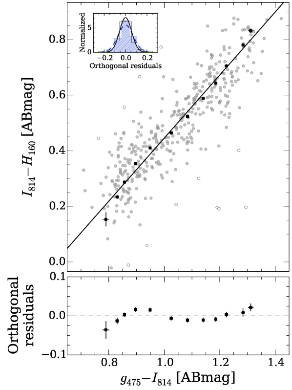
Figure 14.— Optical-NIR $I_{814}{-}H_{160}$ vs. purely optical $g_{475}{-}I_{814}$ color. The upper panel shows the color-color plane for individual GCs (solid and open gray points) and the modal (most probable) values within twelve bins (dark points with error bars) along with the bisector line (solid black line). Outlier rejection was done by an iterative $3\sigma$-clipping procedure based on minimizing the orthogonal distances of the data points from the linear bisector fit assuming normal distributions, as shown in the inset box (see Section 4.3 for details). The filled gray circles are the final data points after outlier rejection, while the open circles show rejected outliers. The blue dashed curve in the inset box is a normal distribution with $\sigma_{\rm initial}=0.071$ for the light-blue shaded histogram before clipping. The black solid curve in the inset box is a normal distribution with $\sigma_{\rm final}=0.056$ mag for the black hatched histogram after clipping. The bin width along the bisector line was chosen to be $3\sigma_{\rm final}$, and the bin spacing is half of the bin width. The lower panel shows the orthogonal deviations (black squares with error bars) of the twelve binned data points with respect to the best-fit line in the upper panel. The plotted points indicate the modal values within each bin.

Figure 14 shows $I_{814}{-}H_{160}$ as a function of $g_{475}{-}I_{814}$ for the matched sample of GC candidates in NGC 4874. We plot only objects in the $23.0<I_{814}<25.0$ mag range, where the color errors are small and the optical bimodality is most pronounced. The figure shows the best-fit bisector line, i.e., the linear relation that minimizes the orthogonal squared deviations, with 3-$\sigma$ clipping; the clipped points are plotted as open circles. The inset box in Figure 14 shows that a normal distribution with dispersion $\sigma\approx 0.06$ mag provides a good representation of the orthogonal color residuals after clipping. In order to study deviations from a linear color-color relation, we grouped the data into twelve bins along the bisector line; the black squares in the upper panel of Figure 14 show the modal locations within each bin, and the lower panel shows the orthogonal deviations of these bins from the linear relation. Eight of the twelve points deviate significantly from the linear relation, following an inflected, or “wavy,” locus at least qualitatively similar to the results found in other studies of the relations between optical and optical-NIR GC colors using high-quality photometric data sets (e.g., Blakeslee et al. 2012; Chies-Santos et al. 2012; Cantiello et al. 2014).

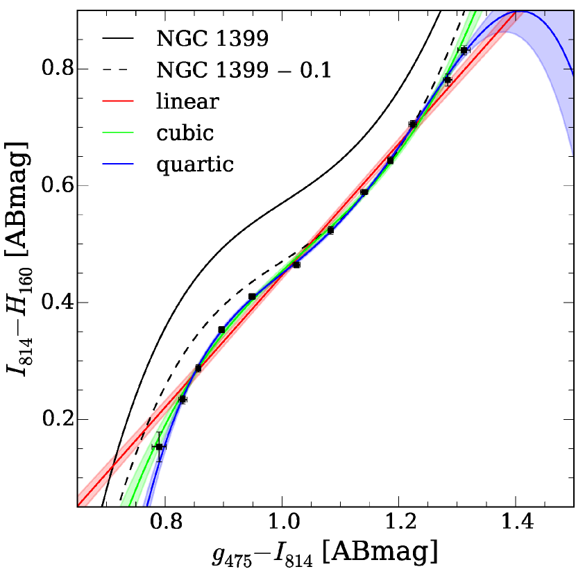
Figure 15.— $I_{814}{-}H_{160}$ vs. $g_{475}{-}I_{814}$ color-color relation with weighted fits that minimize the squared orthogonal distances of the binned data points (black squares, same as plotted in the upper panel of Figure 14). The coefficients of each fit are given in the text. The 1-$\sigma$ ranges of the various fits are indicated with shaded regions. The black solid curve shows the relation from Blakeslee et al. (2012) and the black dashed curve indicates the relation shifted by $-0.1$ mag in $I_{814}{-}H_{160}$ (see text).

The binned modal values of the relation between $I_{814}{-}H_{160}$ and $g_{475}{-}I_{814}$ are again shown in Figure 15, along with several different polynomial fits. Similar to our previous work (Blakeslee et al. 2012), the fits are robust orthogonal regressions, weighted by the uncertainties on the individual binned values; we also show the 1-$\sigma$ uncertainty regions around the fits. The equations for the plotted linear, cubic, and quartic fits are, respectively:

$$I_{814}{-}H_{160} = (-0.68\pm 0.04)+(1.13\pm 0.04)x\,,$$ (9)

$$I_{814}{-}H_{160} = (-7.28\pm 1.53)+(20.60\pm 4.45)x$$ (10)

$$+ (-18.91\pm 4.28)x^{2}+(6.05\pm 1.36)x^{3}\,,$$

$$I_{814}{-}H_{160} = (-37.11\pm 6.17)+(136.11\pm 23.59)x$$ (11)

$$+ (-185.27\pm 33.60)x^{2}+(111.68\pm 21.12)x^{3}$$

$$+ (-24.95\pm 4.94)x^{4}\,,$$

where $x\equiv g_{475}{-}I_{814}$. Both the cubic and quartic polynomials provide statistically acceptable (within ${\sim\,}1\sigma$) descriptions of the data over the applicable domain $0.8\lesssim g_{475}{-}I_{814}\lesssim 1.3$, while the linear fit is rejected with more than 99.9% probability. Thus, the relation is nonlinear to a high degree of significance.

The quartic fit derived for globular clusters in the Fornax cD galaxy NGC 1399 (Blakeslee et al. 2012) is also plotted in Figure 15. Unlike in the present analysis, the 3-pixel aperture magnitudes from that study were not aperture corrected. This is a small effect for $g_{475}{-}I_{814}$ because both $g_{475}$ and $I_{814}$ are measured on ACS data with the same pixel scale and similar PSFs; thus, the differential aperture correction between the two bands is small. However, it is a much larger effect for $I_{814}{-}H_{160}$ because the stacked WFC3/IR images have twice the pixel scale of the stacked ACS images, and GCs are significantly resolved at the 20 Mpc distance of the Fornax cluster. Assuming King model profiles with the range of half-light radii for GCs in the ACS Fornax Cluster Survey (Masters et al. 2010), we find that the correction in $I_{814}{-}H_{160}$ would be in the range of $\sim\,$0.05 to $\sim\,$0.1 mag. Figure 15 shows that shifting the uncorrected 3-pix aperture color relation for NGC 1399 by 0.1 mag provides an approximate (though not statistically acceptable) match to the NGC 4874 relation. This remaining disagreement may result from still larger differential aperture effects at the blue end, where GCs tend to have larger sizes (Jordán et al. 2005; Masters et al. 2010), and/or intrinsic differences in the color-color relations and the underlying color-metallicity relations. Usher et al. (2015) found that there are significant differences in the $g{-}i$ color-metallicity relations for different galaxies. We plan to address this issue fully in a future paper presenting the HST optical-IR colors of GCs in a larger sample of Virgo and Fornax cluster galaxies, including detailed modeling of the differential aperture effects at these more nearby distances. For now, we conclude that the relation between $g_{475}{-}I_{814}$ and $I_{814}{-}H_{160}$ for GCs in NGC 4874 appears to have less extreme curvature than our previously published relation for NGC 1399, but the deviation from a purely linear relation remains highly significant.

4.4. Radial Distributions

The spatial distributions of GCs around galaxies and within galaxy clusters can provide information on the buildup of galaxy halos and cluster dynamical histories (e.g., Moore et al. 2006; Mackey et al. 2010; Lee et al. 2010; Keller et al. 2012). Evidence for sizable populations of IGCs, objects bound to the overall cluster potential rather than any individual galaxy, has been found in several massive galaxy clusters, including Virgo (Lee et al. 2010; Durrell et al. 2014), Coma (Peng et al. 2011), Abell 1185 (West et al. 2011), and Abell 1689 (Alamo-Martínez et al. 2013). Numerical studies (Bekki & Yahagi 2006; Smith et al. 2013, 2015; Mistani et al. 2016) find that dwarf galaxies can lose substantial fractions of their GC systems to the larger cluster environment, but they come to varied conclusions regarding whether the bulk of the IGC population results from stripping of dwarfs or the outskirts of more massive galaxies. Peng et al. (2011) found an extensive population of IGCs in the center of the Coma cluster. Because these IGCs showed a significant tail of red GCs comprising roughly 20% of the population, the authors concluded that a sizable fraction of the IGCs originated in massive galaxies, rather than from disrupted dwarfs.

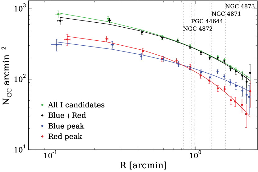
Figure 16.— Number densities of GC candidates within the magnitude range $23.0<I_{814}<26.0$ mag as a function of galactocentric radius $R$ from NGC 4874. The color-coded points represent number density estimates within fixed $10\arcsec$ annuli for different GC subsamples as described in the legend. The values are plotted at the locations of the median galactocentric radius of the GCs within each bin. The horizontal error bars represent the standard deviations of the radial positions within each annulus. The vertical error bars indicate the Poisson errors on the counts, i.e., $\sqrt{N}/$(effective area), within each annulus. The best-fit Sérsic profiles for each subsample are displayed as color-coded curves. The labeled vertical dotted lines indicate the distance from NGC 4874 to the four nearest surrounding galaxies. The half size of the apparent isophotal diameter $\rm D_{25}$ to $\mu_{B}=25.0$ mag/arcsec² (de Vaucouleurs et al. 1991) of NGC 4874 is shown as a vertical dashed line.

In order to quantify the spatial distribution of the GCs, and differences between the red and blue subcomponents, we analyzed the projected surface number density profiles of the ACS GC candidates in the $23.0<I_{814}<26.0$ mag range as a function of galactocentric radius $R$. (Note that we have not integrated the observed counts over an assumed GCLF, in contrast to Peng et al. 2011.) From the center of NGC 4874 to $R=150\arcsec$, the GCs were binned within fixed radial annuli of $10\arcsec$ width. The number of GCs within each annulus was normalized by the effective area of the annulus to get the number densities, and these are plotted against $R$ in Figure 16, along with their Poisson-based uncertainties. We fitted the number densities with the commonly used Sérsic (Sérsic 1963) profile:

$$N_{\rm GC}(R)\,=\,N_{\rm e}\,\exp\left\{-b_{n}\left[\left(\frac{R}{R_{\rm e}}\right)^{1/n}-\,1\right]\right\}\,,$$ (12)

where $N_{\rm e}$ is the projected number density at the effective radius $R_{\rm e}$, $n$ is the Sérsic index, and the constant $b_{n}=1.9992n-0.3271$ (Graham & Driver 2005). We have not fitted a background level because the radial coverage of our data is not wide enough to estimate it. Based on Peng et al. (2011), the expected background of point-like sources at HST/ACS resolution over this magnitude range is more than an order of magnitude below the number densities in our outermost bins (and more than two orders of magnitude below the innermost bins), even when the GCs are split into blue and red groups.

The Sérsic fits to the full radial ranges are shown in Figure 16; the reduced $\chi^{2}$ values for these fits are typically $\sim 0.9$, indicating that the fits provide reasonable descriptions of the data over these radial ranges. For the full color-selected sample of GCs with $0.5<g_{475}{-}I_{814}<1.6$ (plotted as black points in Figure 16), we derive a Sérsic index $n_{\rm B+R}=1.5\pm 0.3$ with an effective radius of $R_{\rm e,B+R}=4\farcm 2\pm 1\farcm 5$, corresponding to $122\pm 44$ kpc. Peng et al. (2011), using the shallower ACSCCS data, but covering a larger area of the Coma cluster, found $n=1.3\pm 0.1$, $\ref{=}2\farcm 2\pm 0\farcm 1$, corresponding to $62\pm 2$ kpc. Our value of $n$ agrees closely with this ACSCCS value, while our LABEL:is larger by a factor of $2.0\pm 0.7$, or a $1.4\sigma$ discrepancy. Because our $g_{475}$ imaging is significantly less deep than $I_{814}$, and could potentially affect the completeness of innermost bins, we also fitted the number densities for all the $I_{814}$-selected GC candidates over the same $23.0<I_{814}<26.0$ mag range, but without matching to the $g_{475}$ detections. The resulting densities are represented by green points in Figure 16; as expected, they only differ at the 1-$\sigma$ level for the innermost point. Our Sérsic fit to this sample of “all” $I_{814}$-selected GCs gives $n_{\rm all}=2.0\pm 0.4$, $R_{\rm e,all}=3\farcm 0\pm 0\farcm 7$, or $85\pm 21$ kpc. For this case, LABEL:agrees to better than 1.1$\sigma$, while $n$ differs by 1.7$\sigma$. Given the differences in depth and area for these fits, the level of agreement with the ACSCCS study is reasonable.

Peng et al. (2011) chose not to fit the blue and red GC components individually; this was in part because the separation between the two color components varied with position over the large area that they studied. For instance, they found that the blue peak of the GC population within $R<50$ kpc of NGC 4874 occurred between the locations of the blue and red peaks in the GC color distribution at larger radius. Since our deeper imaging data are limited to this one central pointing, we here examine the radial distributions of the blue and red GCs separately, using the color at the local minimum (approximately $g_{475}{-}I_{814}=1.0$) of the nonparametric kernel density estimate shown in Figure 12 to divide the GCs into “blue” and “red” subpopulations. Fitting each of these color components with Sérsic profiles, we find $n_{\rm B}=1.9\pm 0.7$, $R_{\rm e,B}=7\farcm 0\pm 6\farcm 3$, $n_{\rm R}=1.2\pm 0.2$, $R_{\rm e,R}=1\farcm 6\pm 0\farcm 2$ for the blue and red GCs, respectively.

The large uncertainty for the blue peak subpopulation is mainly due to the fact that the effective radius is apparently much larger than our field of view. The large LABEL:for the blue GC distribution is likely related to the very extended, mainly blue IGC population in Coma (Peng et al. 2011). However, it is also related to the mainly blue populations of GCs around the lower luminosity, but still bright, elliptical galaxies in this field. Figure 16 indicates the radial locations of several neighboring galaxies. The density of blue GCs appears to jump upward near the radii where NGC 4871 and NGC 4873 are located. While these galaxies are bright enough to harbor some red GCs, the mean color of these GCs would be significantly bluer than those of NGC 4874 (e.g., Peng et al. 2006), meaning that some of the smaller neighbors’ red GCs would fall within the range of the blue GCs for NGC 4874. Moreover, the reddest GCs in these neighboring galaxies would be restricted to small galactocentric radii, where the completeness of our $g_{475}$ data suffers. The GCs at larger radii within these galaxies are overwhelmingly blue.

Because there is an inherent covariance between $n$ and LABEL:for Sérsic model fits when the measurements do not extend clearly beyond LABEL:, we have refitted the various GC samples with $n$ fixed at 2.0. To avoid concern over possible incompleteness near the bright galaxy center, we also omit the central radial bin for these fits. With these constraints, we then find: $R_{\rm e,all}=4\farcm 2\pm 0\farcm 3$, $R_{\rm e,B+R}=4\farcm 2\pm 0\farcm 3$, $R_{\rm e,B}=7\farcm 2\pm 1\farcm 2$, and $R_{\rm e,R}=2\farcm 6\pm 0\farcm 2$. Thus, when $n$ is fixed and the central bin is omitted, matching with the $g_{475}$ detections and limiting the color range does not change the resulting profile. However, we continue to find that the effective radius of the radial distribution of the blue GCs is significantly larger than that of the red GCs. Again, this is in part due to the contribution of blue GCs from NGC 4871, NGC 4873, and other galaxies. It is also consistent with the radially declining fraction of red GCs found by Peng et al. (2011) over a larger area of the Coma core, and many other studies that find the red GCs are more concentrated in giant ellipticals and within galaxy clusters (e.g., Faifer et al. 2011; Durrell et al. 2014).

4.5. Two-Dimensional Spatial Distribution

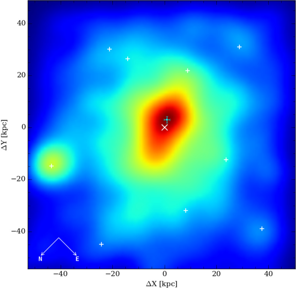
Figure 17.— Example smoothed two-dimensional surface density map of the spatial distribution of GCs from the $I$-band photometry in the range $23.0<I_{814}<26.0$ mag (color indicates surface number density of GCs). The grid size of the two-dimensional histogram is 50 pix with a Gaussian smoothing kernel of $\sigma=4$ grid spacings for this example map; many other grid sizes and smoothings were explored. The white $\times$ symbol marks the center position of NGC 4874 from IRAF ELLIPSE fitting and the cyan point with error bars marks the average center of the GC population. The small white $+$ symbols mark the locations of nine surrounding galaxies.

In order to investigate possible spatial differences between the distributions of the stellar light and GCs in NGC 4874, we constructed two-dimensional smoothed spatial number density maps of the GCs. For this purpose, we used GC candidates selected only from the $I_{814}$ photometry, i.e., the “All I candidates” sample in Figure 16, since completeness may become a problem near the center of the galaxy for the ACS/F475W image. However, we have also repeated the full two-dimensional analysis using the matched F814W/F475W sample, and the results do not change in any significant way. To characterize the two-dimensional GC distribution, we divided the ACS field into two-dimensional grids with various grid sizes: 40, 50, 60, 70, 80, 90, and 100 pix on a side (recall the scale is 0$\farcs$05 pix^-1 for our ACS imaging) and calculated the number density of GCs within each grid cell. The resulting bi-dimensional histograms were then smoothed with Gaussian kernels with varying standard deviations of $\sigma=2$, 3, and 4, in units of the grid spacing. Surprisingly, the peaks of these smoothed two-dimensional GC density distributions generally do not encompass the luminosity center of NGC 4874, i.e., the GCs in the inner region of this field have an off-centered spatial distribution with respect to NGC 4874. An example smoothed GC surface density map (50 pix grid size with $\sigma=4$ grid smoothing) is shown in Figure 17 with the locations of the ten brightest galaxies marked. As evident in the figure, the peak of the GC density distribution is displaced towards the south/southwest with respect to the center of NGC 4874.

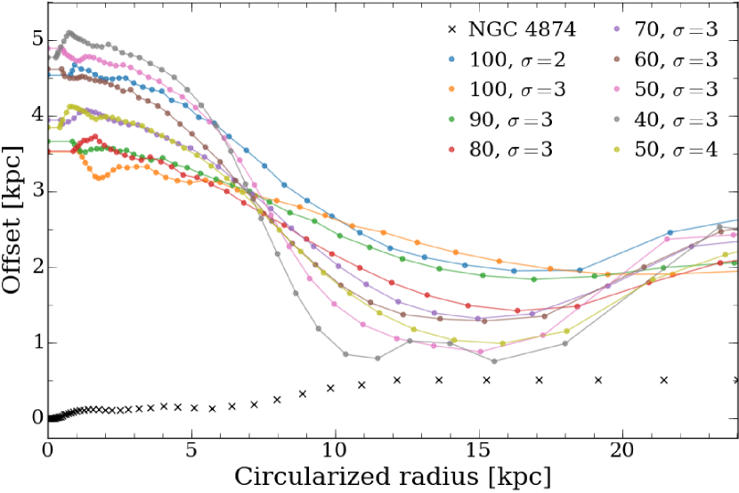
Figure 18.— Offset distance between the peak of NGC 4874’s starlight and the centers of elliptical isophotes of various circularized radii $r_{\rm cir}$. The elliptical isophotes (or isodensity contours) are fitted to multiple different 2-D representations (round points of various colors indicating the different 2-D binnings and smoothing scales) of the GC number density distribution, as well as to the galaxy light itself (black crosses). For the GC density distribution, the grid size (in pixels) of the spatial binning and the Gaussian smoothing $\sigma$ (in units of grid spacing) are indicated in the legend. The circularized radius is defined as $r_{\rm cir}=a\sqrt{1{-}\epsilon}$, where $a$ is the semi-major axis of each elliptical isophote (or isodensity contour) and $\epsilon$ is its ellipticity. Regardless of the factor-of-two range in grid size and smoothing scale, we find that the central peak of the elliptical model of the GC density distribution is offset by 3–5 kpc (6″ to 10″) with respect to the central peak of NGC 4874 itself. At large radii, beyond $\sim 10$ kpc, the center of the elliptical GC isodensity contours approach to within about 1.5 kpc of the luminosity center of NGC 4874.

To quantify the centroid of the GC distribution, we fitted elliptical isophotes (representing GC number isodensity contours) to the smoothed density maps using the IRAF ELLIPSE task. The distance from the luminosity center of NGC 4874 to the center of each ellipse is plotted in Figure 18 as a function of the circularized radius of each isophote $r_{\rm cir}=a\sqrt{1-\epsilon}$, where $a$ is the semi-major axis and $\epsilon$ is the ellipticity of each ellipse. We estimated the statistical significance of the centroid offsets by bootstrap resampling of the GC spatial density distribution 10,000 times before applying the two-dimensional smoothing. Figure 18 shows that, regardless of the particular smoothing, the centroid of the GC density distribution is displaced from the galaxy center by $4\pm 1$ kpc (about 8″) towards the south/southwest from the center of stellar light distribution. However, on larger scales, $r_{\rm cir}\gtrsim 10$ kpc, the centers of the GC isodensity contours approach within $\sim 1$ kpc of the center of the galaxy isophotes. We note that Kim et al. (2013) also reported an offset (of $\sim 3$ kpc) for the center of the GC system around NGC 1399, the cD galaxy in the Fornax cluster.

Most likely this displacement in the centroid of the GC system is related to dynamical interactions within this very rich environment. We note that NGC 4889, the brightest galaxy in the Coma cluster, is located approximately 200 kpc to the east, and thus does not appear to be associated with the observed small offset of NGC 4874’s GC system. However, the offset does align closely with the direction towards NGC 4872, an S0 galaxy with a prominent bar. At a separation of only 0$\farcm$82, or 24 kpc, NGC 4872 is the closest of the bright neighboring galaxies, and its velocity (from NED) differs by only $17\pm 4$ km s^-1 from NGC 4874. Despite its luminosity, NGC 4872 does not have an obvious GC system of its own (unlike NGC 4871 and NGC 4873). It would be interesting to explore through dynamical modeling if the observed offset of the NGC 4874 GC distribution could be related to dynamical interaction with NGC 4872.

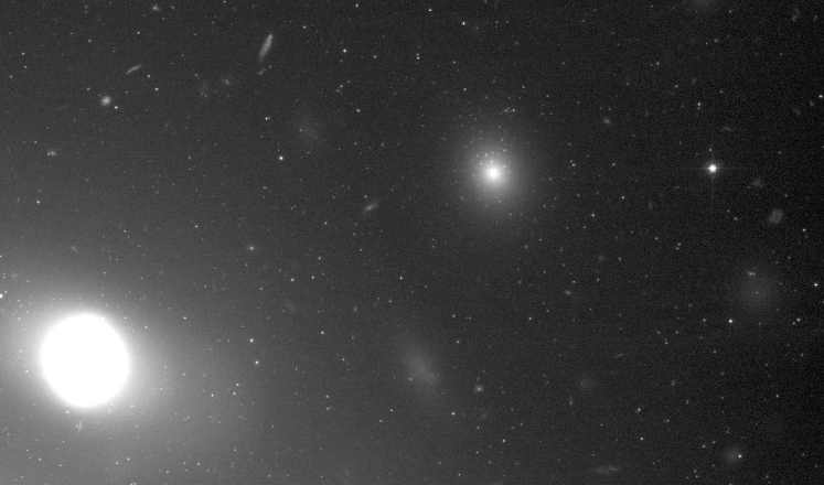
Figure 19.— $84\arcsec{\,\times\,}50\arcsec$ ($\sim 40$ kpc${\,\times\,}24$ kpc) section near the top right corner of our deep F814W image (shown in full in Figure 1 (a)). The brightest galaxy here, near the lower left corner in this subimage, is the SB0 galaxy NGC 4872 (labeled in Figure 1 (a)). The dwarf elliptical galaxy just to the upper right of center in this subimage is SDSS J125935.18$+$275605.0. It contains a sizable population of GCs with an asymmetric spatial distribution. Interestingly, this dE galaxy has a very high relative velocity of $-2660\pm 160$ km s^-1 with respect to the cluster mean; this is about 2.5 times the cluster velocity dispersion. Several extremely diffuse galaxies, like those found in other recent studies, are also evident in this field.

4.6. A Dwarf Elliptical with an Asymmetrical GC System

In the course of our analysis of the galaxy light distributions, we noticed one particular dwarf elliptical (dE) galaxy 1$\farcm$47 from NGC 4874 that seemed relatively rich in GCs, but the GC distribution appeared strikingly asymmetrical. Searching its coordinates in NED, we found that the galaxy was catalogued in the Sloan Digital Sky Survey (SDSS) and is designated SDSS J125935.18$+$275605.0; for convenience, we refer to it hereafter as SDSS J125935. This is the faintest of the ten galaxies in our ACS images for which we performed isophotal modeling, and it lies near the top right corner of our ACS field (outside our WFC3/IR imaging area); see the galaxy model panel in Figure 1. Figure 19 shows an $84\arcsec\times 50\arcsec$ cutout of the region around this galaxy in our $I_{814}$ image; the much brighter galaxy at lower left in this figure is NGC 4872, discussed above. Several fainter, more diffuse, objects in this field appear similar to the extremely diffuse galaxies first systematically catalogued in the Coma cluster by van Dokkum et al. (2015), and shown from deep Subaru imaging to be ubiquitous throughout the Coma cluster (Koda et al. 2015). The image also shows that the density of point sources around the dE SDSS J125935 is not symmetric about the galaxy’s center.

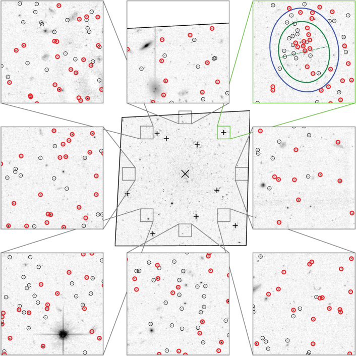
Figure 20.— Spatial distributions of GCs around the dE galaxy SDSS J125935.18$+$275605.0 and in seven control fields at the same projected distance from the cD galaxy NGC 4874. Each of the small fields is $20\arcsec\times 20\arcsec$ in size, except the top center field, which is $20\arcsec\times 15\arcsec$ because of its proximity to the image edge. The dE has been subtracted via isophotal modeling; the larger (blue) ellipse marks the outermost isophote for which we were able to constrain the galaxy’s ellipticity and position angle in our F814W imaging; it has semi-major and semi-minor axes of 4.0 kpc and 3.2 kpc, respectively. For comparison, the green ellipse indicates the $r=25$ mag arcsec^-2 isophote catalogued in the SDSS; the dashed line marks the minor axis of this ellipse. Objects within red circles are GC candidates with $I_{814}<26$ mag, while those within black circles have $26.0<I_{814}<26.9$ mag (see text). The GCs associated with SDSS J125935.18$+$275605.0 tend to fall towards one side of the galaxy, in the direction opposite of NGC 4874; the outer isophote also appears to be offset in this direction. Given this dE galaxy’s very high velocity relative to Coma, its proximity to the cluster dynamical center, and its asymmetrically distributed GC system, it may be passing through the core of the cluster on its first infall and being stripped of much of its GC system.

Figure 20 further illustrates the spatial asymmetry of the GC distribution in a $20\arcsec\times 20\arcsec$ box around this dE by comparing it to seven “control” fields of the same size and at the same radius with respect to the cD galaxy NGC 4874. In the figure, GCs in the matched F475W+F814W sample with $I_{814}<26.0$ mag are shown with red circles, while those with $26<I_{814}<26.9$ mag (i.e., down to the expected GCLF turnover) are shown with smaller black circles. Although we have found that the completeness of the F475W detections is lower near the center of NGC 4874 and the other bright ellipticals, the surface brightness of SDSS J125935 is low enough that completeness is not a serious issue to this magnitude. The dE itself has been subtracted using our isophotal model. The green ellipse shows the $r=25$ mag arcsec^-2 isophote from the SDSS, as reported by NED, and the dashed line marks the minor axis of this ellipse. The blue ellipse indicates the outermost isophote for which we were able to constrain the galaxy’s ellipticity and position angle from our deep F814W image; it has a semi-major axis of 8$\farcs$25 and an ellipticity of 0.192. At the distance of Coma, this translates to semi-major and semi-minor axes of 4.0 and 3.2 kpc, respectively.

For the GCs with $I_{814}<26.0$ mag, 9 of the 11 inside the green ellipse lie to one side of the minor axis; the probability of this occurring by chance is 6.5%, based on Monte Carlo tests. However, the asymmetry is not limited to the brighter GCs; for those with $I_{814}<26.9$ mag (red plus black circles), 17 of 23 lie to one side, which has a random probability of 3.5%. Considering the larger blue ellipse, 12 of 15 GCs with $I_{814}<26$ mag, and 23 of 31 GCs with $I_{814}<26.9$ mag, lie to one side of the minor axis; these have random probabilities of 3.5% and 1.1%, respectively. Thus, the asymmetry is significant with $\sim 99$% confidence. It is evident from Figure 20 that the outermost galaxy isophote is also offset slightly (centroid shift of 0$\farcs$4) in the same direction as the GCs.

We can estimate the size of the GC population in SDSS J125935 from the $31\pm 5.6$ GC candidates (the error is based on Poisson statistics) with $I_{814}<26.9$ mag within the blue ellipse in Figure 20. This ellipse has an area of 172.9 arcsec², and based on the density of GC candidates in the control fields, we would expect $14\pm 4$ contaminants (mostly GCs belonging to NGC 4874) in this area. The difference is $17\pm 7$, which represents the number of GCs associated with SDSS J125935 brighter than the GCLF turnover. For the total population, assuming a symmetric GCLF, we double this number to obtain $34\pm 14$ GCs. To estimate the specific frequency $S_{N}$ (number per unit $V$ luminosity; Harris & van den Bergh 1981), we measure the galaxy magnitude within the same elliptical aperture for consistency and find $I_{814}=17.46\pm 0.01$ mag. The galaxy color is $g_{475}{-}I_{814}=1.072\pm 0.018$ mag. Both of these values are on the AB system and are corrected for Galactic extinction. Using empirical transformations from Blakeslee et al. (2009, 2012), this color corresponds to $g_{475}{-}z_{850}\approx 1.26$ mag (typical of many dEs in the ACS Virgo Cluster Survey) and $V{-}I\approx 1.10$ mag, where the latter value is on the standard Vega-based system. To get the absolute $V$ magnitude, we subtract 0.42 mag from $I_{814}$ to convert to the Vega system, then subtract the distance modulus $(m{-}M)=35.0$, and finally add the estimated $V{-}I$ to obtain $M_{V}=-16.86$ mag. The specific frequency is then $S_{N}=6.1\pm 2.6$ (the error includes an estimated 10% uncertainty on the galaxy luminosity). While this $S_{N}$ would be above average for a large galaxy, it is well within the range for dEs of similar luminosity in the Virgo cluster (Peng et al. 2008).

Remarkably, SDSS J125935 has a heliocentric radial velocity of $4193\pm 154$ km s^-1, measured by Biviano et al. (1995). This is nearly 3000 km s^-1 less than the velocity of $7176\pm 3$ km s^-1 for NGC 4874 (Trager et al. 2008). According to Colless & Dunn (1996), the main component of the Coma cluster centered on NGC 4874 has a mean velocity ${\langle}v{\rangle}=6853\pm 54$ km s^-1 and line-of-sight velocity dispersion $\sigma_{\rm Coma}=1082$ km s^-1. Thus, SDSS J125935 has a relative velocity of $-2660\pm 160$ km s^-1 with respective to the cluster mean, or $-(2.5\pm 0.2)\sigma_{\rm Coma}$. Numerical simulations indicate that dEs at such small clustercentric radii and high relative velocities are likely to be on their first infall into the cluster core (Smith et al. 2013, 2015). The same simulations show that dwarfs that pass through the cluster centers can lose a large fraction, even the majority, of their GC systems (see also Aguilar & White 1986 for illustrations of how similar encounters can result in asymmetric distributions of GC-like test masses).

We suggest that SDSS J125935 is a dwarf elliptical with a relatively rich GC system, similar to some dEs in Virgo, that has recently fallen at high velocity into the core of the Coma cluster and is undergoing stripping of its GC system. Unfortunately, it is presently unfeasible to measure spectroscopic velocities for the surrounding point sources to determine what fraction belong to SDSS J125935. This would be another interesting system for detailed dynamical modeling.

5. Summary & Conclusions

We have studied the rich GC system of NGC 4874, the cD galaxy in the core of the Coma cluster of galaxies, using optical HST $g_{475}$ and $I_{814}$ imaging from the ACS/WFC and near-IR $H_{160}$ imaging from WFC3/IR. The GC system of NGC 4874 and the surrounding Coma core was previously studied in $g_{475}$ and $I_{814}$ as part of the ACSCCS (Peng et al. 2011), and we find excellent photometric agreement with that study, but the exposure time of our $I_{814}$ observations is more than seven times that of the ACSCCS imaging, giving a limiting magnitude more than a magnitude fainter in this bandpass. Because we added the ACSCCS $g_{475}$ observations to our own, the stacked $g_{475}$ image has a factor of two more exposure time than the ACSCCS in the overlap region; tests show that our $g_{475}{-}I_{814}$ color measurements have a factor of two smaller errors than those from the ACSCCS. In addition, we include new deep F160W observations, with an exposure time slightly longer than that of $I_{814}$, over the smaller field of the WFC3/IR.

Because the $I_{814}{-}H_{160}$ color for old stellar populations measures red giant branch temperature, it should be sensitive mainly to metallicity, while $g_{475}{-}I_{814}$ also depends on horizontal branch morphology and the location of the main sequence turnoff. Over most of the luminosity range probed by our data, there exists clear bimodality in the distribution of $g_{475}{-}I_{814}$ colors of our selected GC candidates. This optical bimodality can be traced at least to $I_{814}=26$ mag, corresponding to $M_{814}=-9$ mag at the distance of Coma, or $M_{V}\approx-8$ mag for typical GCs. From a Gaussian mixture modeling analysis as a function of magnitude, we find that at the brightest magnitudes, the blue peak exhibits a very strong “tilt” towards redder colors, with a slope ${d(g_{475}{-}I_{814})}/{dI_{814}}=-0.082\pm 0.020$ for $I_{814}<25$ mag. Based on the empirical calibration of metallicity as a function of photometric color from the ACS Virgo Cluster Survey, this corresponds to a very steep mass-metallicity scaling of $Z\propto M_{\rm GC}^{1.4\pm 0.4}$ at these highest masses.

The GMM analysis for the $I_{814}{-}H_{160}$ color distribution is generally less robust than for $g_{475}{-}I_{814}$, especially when the sample is further broken down by magnitude. We therefore instead examined the variation in the overall mean $I_{814}{-}H_{160}$ color in the same magnitude range as for $g_{475}{-}I_{814}$. Again for $I_{814}<25$ mag, we find a steep slope in the mean $I_{814}{-}H_{160}$ color of ${d(I_{814}{-}H_{160})}/{dI_{814}}=-0.093\pm 0.013$. Although there is no empirical relation between $I_{814}{-}H_{160}$ and metallicity for GCs, the linear approximation to the relation between $I_{814}{-}H_{160}$ and $g_{475}{-}I_{814}$ gives ${d(I_{814}{-}H_{160})}/{d(g_{475}{-}I_{814})}\approx 1.1$, which again implies $Z\propto M_{\rm GC}^{1.4}$. Thus, the mean metallicity scaling derived from the full $I_{814}{-}H_{160}$ color range is the same as that found from the blue component of the $g_{475}{-}I_{814}$ color distribution. However, the color-magnitude tilt is not a simple linear relation, and if we extend the linear fit another magnitude fainter to $I_{814}=26$ mag, then the best-fit slopes are roughly a factor of three shallower, giving scalings of $Z\propto M_{\rm GC}^{0.5\pm 0.2}$, consistent with the typical scaling found by Mieske et al. (2010) over a similar mass range.

As a consequence of the tilted color-magnitude relations, the color distributions change as a function of magnitude. Both the $g_{475}{-}I_{814}$ and $I_{814}{-}H_{160}$ distributions appear broad and red, with no evidence for multiple peaks for the brightest GCs at $I_{814}<23$ mag. Fainter than this, $g_{475}{-}I_{814}$ is clearly bimodal, with the prominence of the red peak decreasing at progressively fainter magnitudes. The bimodality is less evident in $I_{814}{-}H_{160}$, but the same general trend occurs, with the histogram transitioning from a redward tilt to being skewed towards the blue at fainter magnitudes. Because of the blue tilt at bright magnitudes and increased measurement error at faint magnitudes, the bimodality is most evident for $23<I_{814}<25$ mag, and we have compared the GMM bimodal decompositions for $g_{475}{-}I_{814}$ and $I_{814}{-}H_{160}$ for the identical sample of GC candidates over this magnitude range. Once the four bluest objects in $I_{814}{-}H_{160}$ are excluded, the red:blue decompositions are consistent, with red fractions $f_{2}$ of $0.61\pm 0.08$ for $g_{475}{-}I_{814}$ and $0.54\pm 0.13$ for $I_{814}{-}H_{160}$.

While the separation of the peaks in units of the peak dispersion is very clear in $g_{475}{-}I_{814}$ with $D=2.88\pm 0.28$, it is less clear in $I_{814}{-}H_{160}$ with $D=2.23\pm 0.26$, even though the separation in magnitudes is essentially identical. The reason for this is that the blue peak is much narrower in $g_{475}{-}I_{814}$, with a dispersion $\sigma_{1}=0.067\pm 0.014$ mag, compared to $\sigma_{1}=0.098\pm 0.013$ mag for $I_{814}{-}H_{160}$, a difference of nearly 50%. For the red peaks, the dispersions are $\sigma_{2}=0.105\pm 0.014$ mag and $\sigma_{2}=0.126\pm 0.017$ mag for $g_{475}{-}I_{814}$ and $I_{814}{-}H_{160}$, respectively. Previous studies of optical GC color distributions (e.g., Peng et al. 2006, 2009; Harris et al. 2016) also found that the blue peak was significantly narrower than the red peak; however, Peng et al. (2006) pointed out that the dispersion in $[{\rm Fe/H}]$ was actually larger for the blue peak because of the steeper variation in metallicity with color for the blue component of the GCs. The differences in the blue and red color dispersions for $g_{475}{-}I_{814}$ as compared to $I_{814}{-}H_{160}$ suggests that the colors follow different color-metallicity relations, despite their nearly identical total range in color. In particular, the metallicity slopes at blue and red colors must be more similar (i.e., weaker nonlinearity) for $I_{814}{-}H_{160}$ than for $g_{475}{-}I_{814}$. Consistent with this, we find that the variation in $I_{814}{-}H_{160}$ with $g_{475}{-}I_{814}$ is nonlinear, with an inflected shape that can be described well by a cubic polynomial.

We have compared the radial distributions of the blue and red GCs over the wider ACS field of view. Consistent with previous studies, we find that the blue GCs follow a more spatially extended radial profile than the red GCs. Interestingly, for this field located in the dense central region of the rich Coma cluster of galaxies, the broader extent of the blue GCs is at least partially the result of the GCs associated with the fainter neighboring early-type cluster galaxies, whose GC systems are predominantly blue, especially at large galactocentric radii. This is consistent with the view that a significant fraction of the blue GCs in the halos of massive galaxies are added through the accretion or stripping of lower luminosity satellite galaxies.

Curiously, the center of the spatial distribution of the GCs in this field is offset by $4\pm 1$ kpc from the center of NGC 4874 itself. This offset does not appear to result from the superposition of the GC population of any neighboring galaxy, but it is likely the signature of past dynamical interaction. The most likely candidate for this is NGC 4872, a bright SB0 galaxy 24 kpc from the center of NGC 4874 with a velocity difference of less than 20 km s^-1. Although NGC 4872 does not have a significant GC population of its own, the 4 kpc displacement in the centroid of the NGC 4874 GC system lies along the line towards NGC 4872. We have also discussed the asymmetry of the GC system of the dE galaxy SDSS J125935, which is projected 42 kpc from NGC 4874, but has a relative velocity of $-2983$ km s^-1 with respect to the cD, and $-2660$ km s^-1 with respect to the cluster mean. The dE has a specific frequency $S_{N}=6.1\pm 2.6$. The likelihood of the asymmetry in its GCs occurring by chance is $\sim 1$%. We suggest that this dE is on an initial high-velocity infall into the cluster core and its GC system is in the process of being stripped.

Interestingly, based on stellar absorption line indices, Trager et al. (2008) concluded that NGC 4874 and neighboring early-type galaxies showed evidence for an intermediate-age stellar population component, which would imply a significant star formation event several billion years ago. For now, it remains a matter of speculation whether this proposed star formation event in the relatively recent past is associated with the spatial offset of the NGC 4874 GCs. It is also unknown whether or not such an event may have produced any significant population of intermediate-age GCs. If so, one would expect the color-metallicity and color-color relations in this field to differ from those in massive galaxies with exclusively old GC populations, as predicted from stellar population models (Yoon & Chung 2009). Usher et al. (2015) have shown that the color-metallicity relations do indeed vary among early-type galaxies, and that this variation appears to correlate with galaxy luminosity and color; further work is needed to understand the detailed causes of these variations.

We are currently carrying out an optical-NIR photometric study of GCs in a much larger set of 16 early-type galaxies in the Fornax and Virgo clusters by cross-matching our HST WFC3/IR data (Jensen et al. 2015) with the published F475W and F850LP catalogs from the ACS Fornax and Virgo Cluster Surveys (Jordán et al. 2009, 2015). Because these galaxies cover a large range in luminosity and color, this sample will shed light on whether optical/NIR color-color relations show variations with galaxy type similar to those found by Usher et al. (2015) for the relation between optical color and metallicity estimated from the CaT index, as well as illuminating differences in the ways that different broadband colors trace the underlying metallicity. Unfortunately, existing samples of spectroscopically estimated metallicities for massive early-type galaxies are of inhomogeneous quality, tend to be based on a small number of metal absorption line indices, and often have large uncertainties in excess of $0.5$ dex. A large sample of uniformly high-quality spectroscopic metallicities ($\sigma_{[{\rm Fe/H}]}\sim 0.1$ dex) and ages determined over a broad spectral range for hundreds of GCs spanning the full color range in a nearby cD galaxy (which likely combines GCs from a diverse mix of other cluster galaxies) would be an invaluable resource for the community. Such a sample would allow us to calibrate empirically the detailed forms of the color-metallicity relations from the UV to the NIR, and thus constrain the enrichment histories of more distant galaxies from photometric studies alone; it would also enable crucial tests of the stellar population models. The evolutionary histories of massive galaxies and their surrounding environments are encoded in the properties of the ancient systems of GCs that surround them; decoding these histories remains a major ongoing archaeological effort in extragalactic astronomy.

Table 2The GMM Analysis Results for the Color Distributions Shown in Figures 10, 11, and 12 (full sample)

$I_{814}$	Ntot	$\mu_{1}$	$\sigma_{1}$	$\mu_{2}$	$\sigma_{2}$	$f_{2}$	D	kurt	$p(\chi^{2})$
(1)	(2)	(3)	(4)	(5)	(6)	(7)	(8)	(9)	(10)
$g_{475}{-}I_{814}$ of ACS F814W and F475W matched samples
21.5–23.0	26	1.065$\pm$0.030	0.048$\pm$0.017	1.219$\pm$0.028	0.053$\pm$0.016	0.566$\pm$0.167	3.07$\pm$0.72	$-$1.105	0.566
23.0–24.0	164	0.922$\pm$0.035	0.078$\pm$0.021	1.154$\pm$0.026	0.091$\pm$0.015	0.634$\pm$0.126	2.74$\pm$0.40	$-$0.756	0.003
24.0–25.0	775	0.866$\pm$0.011	0.068$\pm$0.010	1.112$\pm$0.022	0.127$\pm$0.012	0.627$\pm$0.071	2.42$\pm$0.26	$-$0.736	$<$0.001
25.0–26.0	1798	0.839$\pm$0.010	0.071$\pm$0.014	1.090$\pm$0.034	0.190$\pm$0.017	0.702$\pm$0.092	1.75$\pm$0.28	$-$0.557	$<$0.010
23.0–25.0	939	0.873$\pm$0.010	0.071$\pm$0.008	1.123$\pm$0.017	0.119$\pm$0.010	0.624$\pm$0.055	2.55$\pm$0.21	$-$0.775	$<$0.001
$I_{814}{-}H_{160}$ of ACS F814W and WFC3/IR F160W matched samples
21.5–23.0	12	0.638$\pm$0.036	0.102$\pm$0.028	0.914$\pm$0.050	0.026$\pm$0.019	0.161$\pm$0.129	3.71$\pm$1.23	$-$0.854	0.275
23.0–24.0	74	0.400$\pm$0.032	0.071$\pm$0.018	0.633$\pm$0.032	0.088$\pm$0.016	0.603$\pm$0.119	2.92$\pm$0.49	$-$0.899	0.088
24.0–25.0	319	0.397$\pm$0.044	0.138$\pm$0.024	0.675$\pm$0.078	0.110$\pm$0.031	0.271$\pm$0.184	2.24$\pm$0.41	$-$0.483	0.050
25.0–26.0	643	0.419$\pm$0.167	0.202$\pm$0.040	0.769$\pm$0.111	0.138$\pm$0.054	0.152$\pm$0.240	2.02$\pm$0.71	$-$0.111	0.190
23.0–25.0	393	0.399$\pm$0.035	0.133$\pm$0.020	0.660$\pm$0.052	0.108$\pm$0.020	0.330$\pm$0.144	2.17$\pm$0.32	$-$0.499	0.030

Note. — Column lists: (1) $I_{814}$ AB magnitude range; (2) total number of objects in the analyzed sample; (3) mean and uncertainty of the first mode in the double Gaussian mixture model; (4) standard deviation and uncertainty of the first mode; (5) mean and uncertainty of the second mode; (6) standard deviation and uncertainty of the second mode; (7) fraction of objects assigned to the second component of the double Gaussian mixture model; (8) separation between the peaks relative to their Gaussian $\sigma$; (9) kurtosis of the distribution; (10) likelihood that the sample was drawn from a single Gaussian distribution.

Table 3The GMM Analysis Results for the Color Distributions Shown in Figure 13 (matched subsample)

Case	Ntot	$\mu_{1}$	$\sigma_{1}$	$\mu_{2}$	$\sigma_{2}$	$f_{2}$	D	kurt	$p(\chi^{2})$
(1)	(2)	(3)	(4)	(5)	(6)	(7)	(8)	(9)	(10)
$g_{475}{-}I_{814}$ of ACS F814W $+$ F475W $+$ WFC3/IR F160W matched samples
$\sigma_{1}\neq\sigma_{2}$	392	0.884$\pm$0.016	0.067$\pm$0.015	1.139$\pm$0.026	0.106$\pm$0.016	0.604$\pm$0.083	2.89$\pm$0.32	$-$0.986	$<$0.001
$\sigma_{1}=\sigma_{2}$	392	0.911$\pm$0.009	0.087$\pm$0.004	1.168$\pm$0.009	0.087$\pm$0.004	0.493$\pm$0.031	2.94$\pm$0.20	$-$0.986	$<$0.001
$I_{814}{-}H_{160}$ of ACS F814W $+$ F475W $+$ WFC3/IR F160W matched samples
$\sigma_{1}\neq\sigma_{2}$	392	0.399$\pm$0.031	0.133$\pm$0.018	0.663$\pm$0.047	0.107$\pm$0.018	0.324$\pm$0.128	2.18$\pm$0.29	$-$0.501	0.034
$\sigma_{1}=\sigma_{2}$	392	0.373$\pm$0.015	0.121$\pm$0.008	0.629$\pm$0.019	0.121$\pm$0.008	0.436$\pm$0.054	2.12$\pm$0.28	$-$0.501	0.007

Note. — Column (1) shows whether the double Gaussian mixture is for the heteroscedastic or homoscedastic case. Columns (2)-(10) are the same as in Table 2.

Table 4Same as Table 3 but in different color ranges.

$I_{814}{-}H_{160}$	Ntot	$\mu_{1}$	$\sigma_{1}$	$\mu_{2}$	$\sigma_{2}$	$f_{2}$	D	kurt	$p(\chi^{2})$
(1)	(2)	(3)	(4)	(5)	(6)	(7)	(8)	(9)	(10)
$g_{475}{-}I_{814}$ of ACS F814W $+$ F475W $+$ WFC3/IR F160W matched samples
$-0.022$ to $0.877$	392	0.884$\pm$0.016	0.067$\pm$0.015	1.139$\pm$0.026	0.106$\pm$0.016	0.604$\pm$0.083	2.89$\pm$0.32	$-$0.986	$<$0.001
$0.059$ to $0.877$	390	0.885$\pm$0.018	0.067$\pm$0.016	1.140$\pm$0.026	0.105$\pm$0.016	0.604$\pm$0.087	2.88$\pm$0.30	$-$0.980	$<$0.001
$0.133$ to $0.877$	388	0.885$\pm$0.016	0.067$\pm$0.014	1.139$\pm$0.023	0.105$\pm$0.014	0.609$\pm$0.082	2.88$\pm$0.28	$-$0.978	$<$0.001
$I_{814}{-}H_{160}$ of ACS F814W $+$ F475W $+$ WFC3/IR F160W matched samples
$-0.022$ to $0.877$	392	0.399$\pm$0.031	0.133$\pm$0.018	0.663$\pm$0.047	0.107$\pm$0.018	0.324$\pm$0.128	2.18$\pm$0.29	$-$0.501	0.034
$0.059$ to $0.877$	390	0.368$\pm$0.033	0.111$\pm$0.015	0.627$\pm$0.042	0.119$\pm$0.017	0.461$\pm$0.132	2.25$\pm$0.26	$-$0.667	0.002
$0.133$ to $0.877$	388	0.353$\pm$0.031	0.098$\pm$0.013	0.606$\pm$0.041	0.126$\pm$0.017	0.538$\pm$0.126	2.23$\pm$0.26	$-$0.727	$<$0.001

Note. — Column (1) shows minimum and maximum values of $I_{814}{-}H_{160}$ color for the objects in the sample (the $g_{475}{-}I_{814}$ ranges are not modified). Columns (2)-(10) are the same as in Table 2.

References

- Aguilar & White (1986) Aguilar, L. A., & White, S. D. M. 1986, ApJ, 307, 97
- Alamo-Martínez et al. (2013) Alamo-Martínez, K. A., Blakeslee, J. P., Jee, M. J., et al. 2013, ApJ, 775, 20
- Anderson & Bedin (2010) Anderson, J., & Bedin, L. R. 2010, PASP, 122, 1035
- Bailin & Harris (2009) Bailin, J., & Harris, W. E. 2009, ApJ, 695, 1082
- Beasley et al. (2008) Beasley, M. A., Bridges, T., Peng, E., et al. 2008, MNRAS, 386, 1443
- Bekki & Yahagi (2006) Bekki, K., & Yahagi, H. 2006, MNRAS, 372, 1019
- Bekki et al. (2008) Bekki, K., Yahagi, H., Nagashima, M., & Forbes, D. A. 2008, MNRAS, 387, 1131
- Benítez (2000) Benítez, N. 2000, ApJ, 536, 571
- Bergbusch & VandenBerg (2001) Bergbusch, P. A., & VandenBerg, D. A. 2001, ApJ, 556, 322
- Bertin & Arnouts (1996) Bertin, E., & Arnouts, S. 1996, A&AS, 117, 393
- Biviano et al. (1995) Biviano, A., Durret, F., Gerbal, D., et al. 1995, A&AS, 111, 265
- Blakeslee (1999) Blakeslee, J. P. 1999, AJ, 118, 1506
- Blakeslee et al. (2003) Blakeslee, J. P., Anderson, K. R., Meurer, G. R., et al. 2003, Astronomical Data Analysis Software and Systems XII, 295, 257
- Blakeslee et al. (2012) Blakeslee, J. P., Cho, H., Peng, E. W., et al. 2012, ApJ, 746, 88
- Blakeslee et al. (2009) Blakeslee, J. P., Jordán, A., Mei, S., et al. 2009, ApJ, 694, 556
- Blakeslee & Tonry (1995) Blakeslee, J. P., & Tonry, J. L. 1995, ApJ, 442, 579
- Blakeslee et al. (1997) Blakeslee, J. P., Tonry, J. L., & Metzger, M. R. 1997, AJ, 114, 482
- Bohlin (2012) Bohlin, R. C. 2012, Instrument Science Report ACS 2012-01 (Baltimore, MD: STScI)
- Brodie et al. (2014) Brodie, J. P., Romanowsky, A. J., Strader, J., et al. 2014, ApJ, 796, 52
- Brodie & Strader (2006) Brodie, J. P., & Strader, J. 2006, ARA&A, 44, 193
- Brodie et al. (2012) Brodie, J. P., Usher, C., Conroy, C., et al. 2012, ApJ, 759, 33
- Bruzual & Charlot (2003) Bruzual, G., & Charlot, S. 2003, MNRAS, 344, 1000
- Busko (1996) Busko, I. C. 1996, in ASP Conf. Ser. 101, Astronomical Data Analysis Software and Systems V, ed. G. H. Jacoby & J. Barnes (San Francisco, CA: ASP), 139
- Cantiello & Blakeslee (2007) Cantiello, M., & Blakeslee, J. P. 2007, ApJ, 669, 982
- Cantiello et al. (2014) Cantiello, M., Blakeslee, J. P., Raimondo, G., et al. 2014, A&A, 564, L3
- Carter et al. (2008) Carter, D., Goudfrooij, P., Mobasher, B., et al. 2008, ApJS, 176, 424
- Chiboucas et al. (2011) Chiboucas, K., Tully, R. B., Marzke, R. O., et al. 2011, ApJ, 737, 86
- Chies-Santos et al. (2012) Chies-Santos, A. L., Larsen, S. S., Cantiello, M., et al. 2012, A&A, 539, A54
- Colless & Dunn (1996) Colless, M., & Dunn, A. M. 1996, ApJ, 458, 435
- Côté et al. (2004) Côté, P., Blakeslee, J. P., Ferrarese, L., et al. 2004, ApJS, 153, 223
- Dirsch et al. (2003) Dirsch, B., Richtler, T., Geisler, D., et al. 2003, AJ, 125, 1908
- Dotter et al. (2007) Dotter, A., Chaboyer, B., Jevremović, D., et al. 2007, AJ, 134, 376
- Dotter et al. (2010) Dotter, A., Sarajedini, A., Anderson, J., et al. 2010, ApJ, 708, 698
- Dressler (1980) Dressler, A. 1980, ApJ, 236, 351
- Durrell et al. (2014) Durrell, P. R., Côté, P., Peng, E. W., et al. 2014, ApJ, 794, 103
- Faifer et al. (2011) Faifer, F. R., Forte, J. C., Norris, M. A., et al. 2011, MNRAS, 416, 155
- Forte et al. (2014) Forte, J. C., Vega, E. I., Faifer, F. R., et al. 2014, MNRAS, 441, 1391
- Fruchter et al. (2009) Fruchter, A., Sosey, M., Hack, W., et al. 2009, The MultiDrizzle Handbook, Version 3.0 (Baltimore, MD: STScI)
- Graham & Driver (2005) Graham, A. W. & Driver, S. P. 2005, PASA, 22, 118
- Harris (1987) Harris, W. E. 1987, ApJ, 315, L29
- Harris (2009) Harris, W. E. 2009, ApJ, 699, 254
- Harris et al. (2016) Harris, W. E., Blakeslee, J. P., Whitmore, B. C., et al. 2016, ApJ, 817, 58
- Harris et al. (2013) Harris, W. E., Harris, G. L. H., & Alessi, M. 2013, ApJ, 772, 82
- Harris et al. (2009) Harris, W. E., Kavelaars, J. J., Hanes, D. A., et al. 2009, AJ, 137, 3314
- Harris & van den Bergh (1981) Harris, W. E., & van den Bergh, S. 1981, AJ, 86, 1627
- Harris et al. (2006) Harris, W. E., Whitmore, B. C., Karakla, D., et al. 2006, ApJ, 636, 90
- Hudson et al. (2014) Hudson, M. J., Harris, G. L., & Harris, W. E. 2014, ApJ, 787, L5
- Jedrzejewski (1987) Jedrzejewski, R. 1987, MNRAS, 226, 747
- Jee et al. (2007) Jee, M. J., Blakeslee, J. P., Sirianni, M., et al. 2007, PASP, 119, 1403
- Jensen et al. (2015) Jensen, J. B., Blakeslee, J. P., Gibson, Z., et al. 2015, ApJ, 808, 91
- Jordán et al. (2007) Jordán, A., Blakeslee, J. P., Côté, P., et al. 2007, ApJS, 169, 213
- Jordán et al. (2004) Jordán, A., Blakeslee, J. P., Peng, E. W., et al. 2004, ApJS, 154, 509
- Jordán et al. (2005) Jordán, A., Côté, P., Blakeslee, J. P., et al. 2005, ApJ, 634, 1002
- Jordán et al. (2009) Jordán, A., Peng, E. W., Blakeslee, J. P., et al. 2009, ApJS, 180, 54
- Jordán et al. (2015) Jordán, A., Peng, E. W., Blakeslee, J. P., et al. 2015, ApJS, 221, 13
- Keller et al. (2012) Keller, S. C., Mackey, D., & Da Costa, G. S. 2012, ApJ, 744, 57
- Kim et al. (2013) Kim, H.-S., Yoon, S.-J., Sohn, S. T., et al. 2013, ApJ, 763, 40
- Koda et al. (2015) Koda, J., Yagi, M., Yamanoi, H., & Komiyama, Y. 2015, ApJ, 807, L2
- Koekemoer et al. (2003) Koekemoer, A. M., Fruchter, A. S., Hook, R. N., & Hack, W. 2003, in The 2002 HST Calibration Workshop, ed. S. Arribas, A. M. Koekemoer, & B. Whitmore (Baltimore, MD: STScI), 337
- Kubo et al. (2007) Kubo, J. M., Stebbins, A., Annis, J., et al. 2007, ApJ, 671, 1466
- Lee et al. (1994) Lee, Y.-W., Demarque, P., & Zinn, R. 1994, ApJ, 423, 248
- Lee et al. (2010) Lee, M. G., Park, H. S., & Hwang, H. S. 2010, Science, 328, 334
- Liu et al. (2015) Liu, C., Peng, E. W., Côté, P., et al. 2015, ApJ, 812, 34
- Mackey et al. (2010) Mackey, A. D., Huxor, A. P., Ferguson, A. M. N., et al. 2010, ApJ, 717, L11
- Madrid et al. (2010) Madrid, J. P., Graham, A. W., Harris, W. E., et al. 2010, ApJ, 722, 1707
- Marín-Franch & Aparicio (2002) Marín-Franch, A. & Aparicio, A. 2002, ApJ, 568, 174
- Masters et al. (2010) Masters, K. L., Jordán, A., Côté, P., et al. 2010, ApJ, 715, 1419
- Mieske et al. (2006) Mieske, S., Jordán, A., Côté, P., et al. 2006, ApJ, 653, 193
- Mieske et al. (2010) Mieske, S., Jordán, A., Côté, P., et al. 2010, ApJ, 710, 1672
- Mistani et al. (2016) Mistani, P. A., Sales, L. V., Pillepich, A., et al. 2016, MNRAS, 455, 2323
- Moore et al. (2006) Moore, B., Diemand, J., Madau, P., et al. 2006, MNRAS, 368, 563
- Muratov & Gnedin (2010) Muratov, A. L., & Gnedin, O. Y. 2010, ApJ, 718, 1266
- Ostrov et al. (1998) Ostrov, P. G., Forte, J. C., & Geisler, D. 1998, AJ, 116, 2854
- Peng et al. (2011) Peng, E. W., Ferguson, H. C., Goudfrooij, P., et al. 2011, ApJ, 730, 23
- Peng et al. (2009) Peng, E. W., Jordán, A., Blakeslee, J. P., et al. 2009, ApJ, 703, 42
- Peng et al. (2006) Peng, E. W., Jordán, A., Côté, P., et al. 2006, ApJ, 639, 95
- Peng et al. (2008) Peng, E. W., Jordán, A., Côté, P., et al. 2008, ApJ, 681, 197
- Puzia et al. (2014) Puzia, T. H., Paolillo, M., Goudfrooij, P., et al. 2014, ApJ, 786, 78
- Puzia et al. (2002) Puzia, T. H., Zepf, S. E., Kissler-Patig, M., et al. 2002, A&A, 391, 453
- Richtler (2006) Richtler, T. 2006, BASI, 34, 83
- Schlafly & Finkbeiner (2011) Schlafly, E. F. & Finkbeiner, D. P. 2011, ApJ, 737, 103
- Schlegel et al. (1998) Schlegel, D. J., Finkbeiner, D. P., & Davis, M. 1998, ApJ, 500, 525
- Sérsic (1963) Sérsic, J. L. 1963, BAAA, 6, 41
- Sirianni et al. (2005) Sirianni, M., Jee, M. J., Benítez, N., et al. 2005, PASP, 117, 1049
- Smith et al. (2015) Smith, R., Sánchez-Janssen, R., Beasley, M. A., et al. 2015, MNRAS, 454, 2502
- Smith et al. (2013) Smith, R., Sánchez-Janssen, R., Fellhauer, M., et al. 2013, MNRAS, 429, 1066
- Spitler & Forbes (2009) Spitler, L. R., & Forbes, D. A. 2009, MNRAS, 392, L1
- Strader et al. (2006) Strader, J., Brodie, J. P., Spitler, L., & Beasley, M. A. 2006, AJ, 132, 2333
- Strader & Smith (2008) Strader, J., & Smith, G. H. 2008, AJ, 136, 1828
- Trager et al. (2008) Trager, S. C., Faber, S. M., & Dressler, A. 2008, MNRAS, 386, 715
- Usher et al. (2012) Usher, C., Forbes, D. A., Brodie, J. P., et al. 2012, MNRAS, 426, 1475
- Usher et al. (2015) Usher, C., Forbes, D. A., Brodie, J. P., et al. 2015, MNRAS, 446, 369
- van Dokkum et al. (2015) van Dokkum, P. G., Abraham, R., Merritt, A., et al. 2015, ApJ, 798, L45
- Vanderbeke et al. (2014) Vanderbeke, J., West, M. J., De Propris, R., et al. 2014, MNRAS, 437, 1734
- Wehner et al. (2008) Wehner, E. M. H., Harris, W. E., Whitmore, B. C., et al. 2008, ApJ, 681, 1233
- West et al. (2011) West, M. J., Jordán, A., Blakeslee, J. P., et al. 2011, A&A, 528, A115
- Woodley et al. (2010) Woodley, K. A., Harris, W. E., Puzia, T. H., et al. 2010, ApJ, 708, 1335
- Yoon & Chung (2009) Yoon, S.-J. & Chung, C. 2009, in ESO Astrophysics Symposia, Globular Clusters – Guides to Galaxies, ed. T. Richtler & S. Larsen (Berlin: Springer), 381
- Yoon et al. (2011) Yoon, S.-J., Lee, S.-Y., Blakeslee, J. P., et al. 2011a, ApJ, 743, 150
- Yoon et al. (2011) Yoon, S.-J., Sohn, S. T., Lee, S.-Y., et al. 2011b, ApJ, 743, 149
- Yoon et al. (2006) Yoon, S.-J., Yi, S. K., & Lee, Y.-W. 2006, Science, 311, 1129
- Zaritsky et al. (2014) Zaritsky, D., Colucci, J. E., Pessev, P. M., et al. 2014, ApJ, 796, 71