A block Recycled GMRES method with investigations into aspects of solver performance

Abstract

We propose a block Krylov subspace version of the GCRO-DR method proposed in [Parks et al. SISC 2005], which is an iterative method allowing for the efficient minimization of the the residual over an augmented block Krylov subspace. We offer a clean derivation of the method and discuss methods of selecting recycling subspaces at restart as well as implementation decisions in the context of high-performance computing. Numerical experiments are split into those demonstrating convergence properties and those demonstrating the data movement and cache efficiencies of the dominant operations of the method, measured using processor monitoring code from Intel.

1 Introduction

At the core of many problems in the computational sciences is the need to solve linear systems. It is often the case that one must solve a sequence of systems, and these systems are somehow related. For example, in the context of uncertainty quantification, one has multiple parameter realizations of the same physical model which must be evaluated [30, 31]. In Newton-like iterations, one frequently solves a sequence of linear systems where the coefficient matrix arises from a matrix function evaluated at a sequence of points where consecutive points are close (e.g., density functional theory computations; see [28]). Such sequences of systems also arise in application areas such as topology optimization [61], the modeling of crack propagation in materials [46], and tomography [33]. Furthermore, each linear system often has more than one right-hand side.

One solution strategy is ignore all these relationships and solve all these systems separately, i.e., for each coefficient matrix solve for each right-hand side one at a time. However, it is more efficient to take advantage of the underlying structure of all problems combined. Block Krylov subspace iterative methods [43, 60] have been proposed to solve systems with many right-hand sides, and such methods have also been proposed to accelerate convergence even when there is is only one right-hand side; see, e.g., [13, 43, 44, 58]. Subspace recycling techniques [46] have been proposed to take advantage of relationships between sequences of coefficient matrices.

In this paper, we explore the combination of these two techniques: Block Krylov and recycling. We justify the utility of the resulting method not just with steeper convergence curves but also with carefully constructed performance experiments. Specifically, we measure the runtimes and cache efficiency of key computational kernels to demonstrate the utility of such block methods.

The rest of this paper is organized as follows. In Section 2 we describe the problem being solved and discuss what has been investigated in the literature. In Section 3 we briefly review Krylov subspace methods and their generalization to the block setting as well as recycled GMRES. In Section 4, we extend the recycled GMRES method to the block Krylov subspace setting. We further describe implementation decisions meant to improve the data movement efficiency of the method. In Section 5, we discuss convergence properties and theory of this method. In Section 6, we present experiments. These are divided into two types. The first include simple convergence experiments, demonstrating the competitiveness of these methods for large-scale problems. We then present measurements of how data is moved to and used on the processor for the dominant operations of the method.

2 Background

We wish to efficiently solve a sequence of linear systems

$$\mathbf{A}^{[i]}\mathbf{X}^{[i]}=\mathbf{B}^{[i]},$$ (1)

where the coefficient matrices $\mathbf{A}^{[i]}\in\mathbb{C}^{n\times n}$ are assumed to be non-Hermitian and the right-hand side $\mathbf{B}^{[i]}\in\mathbb{C}^{n\times p}$. For many applications, the matrices $\mathbf{A}^{[i]}$ are large and sparse. Krylov subspace iterative methods have become a standard tool for solving sparse systems such as those arising in (1). In this paper, we consider both the case that $p=1$ and $p>1$. Block Krylov subspace methods (see Section 3.2) have been proposed in the case that $p>1$ and these techniques can also be used to accelerate convergence in the single-vector case that $p=1$, as first suggested in [43] and elaborated upon in [44] and also used in, e.g., [13, 58]. See, e.g., [26] for a nice introduction.

In the case $p=1$, the GCRO-DR method was introduced for the solution of sequences of slowly-changing linear systems. This method allows one to retain important approximate invariant subspace information generated during the solution of the $i$th linear system, and leverage that information to accelerate convergence of the iteration to solve the subsequent $(i+1)st$ system.

Metrics such as amount of data moved and efficiency of cache reuse become more important measures of algorithm performance than simply counting floating point operations; see, e.g., [29, 36]. For example, in the dense linear algebra setting, it has been shown that BLAS-3 matrix-matrix operations (such as multiplying a dense matrix times a block of vectors) demonstrate superior performance over BLAS-2 matrix-vector operations when measured in terms of these data-related metrics. In the sparse linear algebra setting, the dominant operation of most Krylov subspace methods for the case $p=1$ is a sparse matrix-vector multiplication, and in block Krylov subspace methods this is replaced with a sparse matrix-vector multiplication where the block of vectors is often dense. It has been shown that this sparse block operation also demonstrates superior performance to its non-block counterparts in data-related metrics [9, 29]. Given this observation, it is reasonable to develop block recycling methods, and to explore their application to block systems and systems with a single right-hand side augmented with additional vectors not arising from the problem. This will grow the search space more rapidly.

The extension of GCRO-DR and other such methods is a natural one to make. This paper follows from the development of the block GCRO-DR high-performance implementation [47] in the Belos package of the Trilinos project [2]. Based upon this code, the authors of [32] have extended this method to the flexible preconditioning setting and treat the issue of inexact block Krylov subspace breakdown thoroughly. Other such methods have also been extended to the block setting; see, e.g., [15, 35]. In this paper we:

• derive the block version of GCRO-DR, as implemented in [47],

• discuss implementation decisions to favor block operations, including increasing the Krylov subspace block size using random vectors,

• demonstrate performance gains of a block Krylov subspace recycling over its single-vector counterpart,

• demonstrate the superiority of block, sparse matrix operations in terms appropriate data metrics relevant in the high-performance computing context,

• and study the efficiency of block operations specific to the block GCRO-DR setting.

It should be noted that the last two goals are achieved through direct measurement of data movement and cache use efficiency on the processor. Through carefully designed experiments, we are able to show that the cost of applying an operator to a block of vectors is often marginally greater than applying the operator to a single vector in terms of data movement and usage cost metrics. Thus, we show that block methods can offer an accelerated convergence rate while reducing the overall data transmission costs by avoiding data movement bottlenecks in modern hardware architectures.

3 Preliminaries

In many Krylov subspace iterative methods proposed for the case $p=1$, recall that for $\mathbf{A}\in\mathbb{C}^{n\times n}$, we generate an orthonormal basis for the Krylov subspace

$${\mathcal{K}}_{j}(\mathbf{A},\mathbf{u})=\text{span}\left\{\mathbf{u},\mathbf{A}\mathbf{u},\ldots,\mathbf{A}^{j-1}\mathbf{u}\right\}$$ (2)

with the Arnoldi process, where $\mathbf{u}$ is some starting vector. Let $\mathbf{V}_{j}\in\mathbb{C}^{n\times j}$ be the matrix with orthonormal columns generated by the Arnoldi process spanning ${\mathcal{K}}_{j}(\mathbf{A},\mathbf{u})$. Then we have the Arnoldi relation

$$\mathbf{A}\mathbf{V}_{j}=\mathbf{V}_{j+1}\overline{\mathbf{H}}_{j}$$ (3)

for some $\mathbf{u}\in\mathbb{C}^{n}$ with $\overline{\mathbf{H}}_{j}\in\mathbb{C}^{(j+1)\times j}$; see, e.g., [52, Section 6.3] and [57]. Let $\mathbf{x}_{0}$ be an initial approximation and $\mathbf{r}_{0}=\mathbf{B}-\mathbf{A}\mathbf{x}_{0}$ be the initial residual. At iteration $j$, we compute $\mathbf{x}_{j}=\mathbf{x}_{0}+\mathbf{t}_{j}$, where $\mathbf{t}_{j}\in{\mathcal{K}}_{j}(\mathbf{A},\mathbf{r}_{0})$. In GMRES [53], we choose

$$\mathbf{t}_{j}=\underset{\mathbf{t}\in{\mathcal{K}}_{j}(\mathbf{A},\mathbf{r}_{0})}{\text{{\rm argmin}}}\left\|\mathbf{B}-\mathbf{A}(\mathbf{x}_{0}+\mathbf{t})\right\|,$$

and this is equivalent to solving the smaller minimization problem

$$\mathbf{y}_{j}=\underset{\mathbf{y}\in\mathbb{C}^{j}}{\text{{\rm argmin}}}\left\|\overline{\mathbf{H}}_{j}\mathbf{y}-\left\|\mathbf{r}_{0}\right\|\mathbf{e}_{1}^{(j+1)}\right\|,$$ (4)

where we use the notation $\mathbf{e}_{\ell}^{(k)}$ to denote the $\ell$th Cartesian basis vector in $\mathbb{R}^{k}$, and setting $\mathbf{x}_{j}=\mathbf{x}_{0}+\mathbf{V}_{j}\mathbf{y}_{j}$. We call $\mathbf{t}_{j}$ a correction. In restarted GMRES, i.e., (GMRES($m$)), we halt this process at step $m$, discard the matrix $\mathbf{V}_{m}$, and restart with the new initial residual $\mathbf{r}_{0}~{}\leftarrow~{}\mathbf{B}-\mathbf{A}\mathbf{x}_{m}$. This process is repeated until we achieve convergence.

3.1 Recycled GMRES

In this paper, we are discussing the combination of block Krylov methods with subspace recycling, a type of augmented Krylov subspace method which was first so described with that name in [46]. By augmented Krylov subspace, we mean that we compute a correction to the initial approximation not just over a Krylov subspace ${\mathcal{K}}$ but instead over an augmented Krylov subspace of the form ${\mathcal{U}}+{\mathcal{K}}$ where ${\mathcal{U}}$ is available before the start of the iteration. Here we use the expression Recycled GMRES to encompass all augmented Krylov subspace methods derived from the GCRO framework introduced in [17]. There it was shown that such methods can be described as a GMRES iteration applied to the original linear system, left-multiplied with a specially chosen projector. The correction resulting from this iteration is then further modified to get a minimum residual approximation for the original system, cf. Section 3.1. What differentiates the methods within this class is how the augmenting subspace ${\mathcal{U}}$ is computed and updated.

We briefly review the method described in [46]. This algorithm represents the combination of two approaches: those originating from the implicitly restarted Arnoldi method [34], such as Morgan’s GMRES-DR [40], and those descending from de Sturler’s GCRO method [17]. GMRES-DR is a restarted GMRES-type algorithm, where at the end of each cycle, harmonic Ritz vectors are computed, and a subset of them are used to augment the Krylov subspace generated at the next cycle. The GCRO method allows the user to select the optimal correction over arbitrary subspaces. This concept is extended by de Sturler in [18] (and simplified in [10]), where a framework is provided for selecting the optimal subspace to retain from one cycle to the next so as to minimize the error produced by discarding useful information accumulated in the subspace for candidate solutions before restart. This algorithm is called GCROT, and this procedure was referred to as “optimal truncation”. Parks et al. in [46] combine the ideas of [40] and [18] and extend them to a sequence of slowly-changing linear systems and recycling with harmonic Ritz vectors. They call their method GCRO-DR.

Suppose we are solving (1), and we have a $k$-dimensional subspace ${\mathcal{U}}$ which is spanned by vectors recycled either from a previous linear system solve or in the previous iteration cycle and whose image under the action of $\mathbf{A}$ is ${\mathcal{C}}=\mathbf{A}\,{\mathcal{U}}$. Let $\mathbf{P}$ be the orthogonal projector onto ${\mathcal{C}}$. Based upon what is proven in [17] and using the framework discussed in [24] and then later in the thesis [23], the recycled GMRES iteration can be described as a GMRES iteration applied to the consistent projected problem,

$$\left(\mathbf{I}-\mathbf{P}\right)\mathbf{A}\widehat{\mathbf{x}}=\left(\mathbf{I}-\mathbf{P}\right)\mathbf{B}.$$ (5)

If $\mathbf{x}_{0}$ is an initial approximation to the solution of the original problem, then a compatible $\widehat{\mathbf{x}}_{0}$ such that the residual $\widehat{\mathbf{r}}_{0}\in{\mathcal{C}}^{\perp}$ is always cheaply available. We generate the Krylov subspace with respect to the projected operator, ${\mathcal{K}}_{m}\big{(}\left(\mathbf{I}-\mathbf{P}\right)\mathbf{A},\widehat{\mathbf{r}}_{0}\big{)}$. After $m$ iterations, GMRES applied to (5) produces the correction $\widehat{\mathbf{t}}_{m}\in{\mathcal{K}}_{m}\big{(}\left(\mathbf{I}-\mathbf{P}\right)\mathbf{A},\widehat{\mathbf{r}}_{0}\big{)}$. Let $\mathbf{Q}$ be the projector onto ${\mathcal{U}}$ which is orthogonal but with respect to the non-standard inner product induced by the symmetric positive-definite matrix $\mathbf{A}^{\ast}\mathbf{A}$.. By projecting the GMRES correction $\widehat{\mathbf{t}}_{m}$, we get the second correction $\mathbf{s}_{m}=-\mathbf{Q}\widehat{\mathbf{t}}_{m}$ so that the Recycled GMRES method generates at iteration $m$ the approximation

$$\mathbf{x}_{m}=\widehat{\mathbf{x}}_{0}+\widehat{\mathbf{t}}_{m}+\mathbf{s}_{m}$$

where $\mathbf{s}_{m}\in{\mathcal{U}}$ and $\widehat{\mathbf{t}}_{m}\in{\mathcal{K}}_{m}(\left(\mathbf{I}-\mathbf{P}\right)\mathbf{A},\mathbf{r}_{0})$. Equivalently, these corrections also result from enforcing the minimum residual, Petrov-Galerkin condition over the augmented Krylov subspace, i.e.,

$$\mathbf{r}_{m}=\mathbf{B}-\mathbf{A}\mathbf{x}_{m}\perp\mathbf{A}\left({\mathcal{U}}+{\mathcal{K}}_{m}\left((\mathbf{I}-\mathbf{P})\mathbf{A},\mathbf{r}_{0}\right)\right).$$ (6)

At the end of the cycle, an updated ${\mathcal{U}}$ is constructed, the Krylov subspace basis is discarded, and we restart. At convergence, ${\mathcal{U}}$ is saved, to be used when solving the next linear system.

In terms of implementation, Recycled GMRES can be described as a modification of the GMRES algorithm. Let $\mathbf{U}\in\mathbb{C}^{n\times k}$ have columns spanning ${\mathcal{U}}$, scaled such that $\mathbf{C}=\mathbf{A}\mathbf{U}$ has orthonormal columns. Then we can explicitly construct $\mathbf{P}=\mathbf{I}-\mathbf{C}\mathbf{C}^{\ast}$ and $\mathbf{Q}=\mathbf{U}\mathbf{C}^{\ast}\mathbf{A}$. At each iteration, applying $\left(\mathbf{I}-\mathbf{P}\right)$ is equivalent to performing $k$ steps of the Modified Gram-Schmidt process to orthogonalize the new Arnoldi vector against the columns of $\mathbf{C}$. The orthogonalization coefficients generated at step $m$ are stored in the $m$th column of $\mathbf{F}_{m}=\mathbf{C}^{\ast}\mathbf{A}\mathbf{V}_{m}$, and $\mathbf{F}_{m+1}$ is simply $\mathbf{F}_{m}$ with one new column appended. Let $\overline{\mathbf{H}}_{m}$ and $\mathbf{V}_{m}$ be defined as before, but for the projected Krylov subspace ${\mathcal{K}}_{m}\left(\left(\mathbf{I}-\mathbf{P}\right)\mathbf{A},\mathbf{r}_{0}\right)$. Enforcing (6) is equivalent to solving the GMRES minimization problem (4) for ${\mathcal{K}}_{m}\left(\left(\mathbf{I}-\mathbf{P}\right)\mathbf{A},\mathbf{r}_{0}\right)$ and setting

$$\mathbf{s}_{m}=-\mathbf{U}\mathbf{F}_{m}\mathbf{y}_{m}\mbox{\ \ and\ \ }\mathbf{t}_{m}=\mathbf{V}_{m}\mathbf{y}_{m},$$

so that

$$\mathbf{x}_{m} =\mathbf{x}_{0}-\mathbf{U}\mathbf{F}_{m}\mathbf{y}_{m}+\mathbf{V}_{m}\mathbf{y}_{m}=\mathbf{x}_{0}+\begin{bmatrix}\mathbf{U}&\mathbf{V}_{m}\end{bmatrix}\begin{bmatrix}-\mathbf{F}_{m}\mathbf{y}_{m}\\ \mathbf{y}_{m}\end{bmatrix}.$$

This is a consequence of the fact that the Recycled GMRES least squares problem, as stated in [46, Equation 2.13] can be satisfied exactly in the first $k$ rows. This was first shown in [17].

Convergence analysis for augmented Krylov subspace methods has been previously presented in, e.g., [20, 51]. In the context of Recycled GMRES the thesis of Gaul [23] and the references therein is an excellent source on this topic. Further analysis of these methods and of the deflated operator $\left(\mathbf{I}-\mathbf{P}\right)\mathbf{A}$ is presented.

Iterating orthogonally to an approximate invariant subspace to accelerate convergence of GMRES can be justified by the theoretical work in [56]. It was shown that the widely observed two-stage convergence behavior of GMRES, which has been termed superlinear convergence, is governed by how well the Krylov subspace approximates a certain eigenspace. Specifically, when the Krylov subspace contains a good approximation to the eigenspace (call this eigenspace ${\mathcal{S}}$) associated to eigenvalues hindering convergence, we will switch from the slow phase to the fast phase, and convergence will mimic that of GMRES on the projected operator $\mathbf{P}_{{\mathcal{S}}^{\perp}}\mathbf{A}$ where $\mathbf{P}_{{\mathcal{S}}^{\perp}}$ is the orthogonal projector onto ${\mathcal{S}}^{\perp}$. This analysis complements previous discussions of this phenomenon, see e.g., [11, 59].

3.2 Block Krylov subspace methods

The extension of Krylov subspaces and the associated iterative methods to the block Krylov setting has been previously described in, e.g., [26, 43, 60]. Though originally described for solving (1) in the case $p>1$, such methods have also been proposed for accelerating convergence in the case that $p=1$. Here we drop the index $i$ and consider the linear system $\mathbf{A}\mathbf{X}=\mathbf{B}$. Let $\overline{\mathbf{R}}\in\mathbb{C}^{n\times L}$ be a block of $L$ vectors

1

Input : $\mathbf{A}\in\mathbb{C}^{n\times n}$, $\mathbf{V}_{1},\ldots,\mathbf{V}_{m}\in\mathbb{C}^{n\times p}$

Output : The block Arnoldi vector $\mathbf{V}_{m+1}$

2 $\widehat{\mathbf{V}}_{m+1}=\mathbf{A}\mathbf{V}_{m}$

3 for $i=1$ to $m$ do

4       $\mathbf{H}_{i,m}=\mathbf{V}_{i}^{\ast}\widehat{\mathbf{V}}_{m+1}\in\mathbb{C}^{p\times p}$

5       $\widehat{\mathbf{V}}_{m+1}\leftarrow\widehat{\mathbf{V}}_{m+1}-\mathbf{V}_{i}\mathbf{H}_{i,m}$

Define $\mathbf{V}_{m+1}$ and $\mathbf{H}_{m+1,m}$ using reduced QR-factorization $\widehat{\mathbf{V}}_{m+1}=\mathbf{V}_{m+1}\mathbf{H}_{m+1,m}$

Algorithm 3.1 A step of the block Arnoldi algorithm

A block Krylov subspace $\mathbb{K}_{m}(\mathbf{A},\overline{\mathbf{R}})$ is a generalization of the definition of a Krylov subspace with more than one starting vector, i.e.,

$$\mathbb{K}_{m}(\mathbf{A},\overline{\mathbf{R}})={\rm colspan}\left\{\overline{\mathbf{R}},\mathbf{A}\overline{\mathbf{R}},\mathbf{A}^{2}\overline{\mathbf{R}},\ldots\mathbf{A}^{m-1}\overline{\mathbf{R}}\right\},$$

and it is straightforward to show that this definition is equivalent to

$$\mathbb{K}_{m}(\mathbf{A},\overline{\mathbf{R}})={\mathcal{K}}_{m}(\mathbf{A},\overline{\mathbf{r}}^{(1)})+{\mathcal{K}}_{m}(\mathbf{A},\overline{\mathbf{r}}^{(2)})+\cdots+{\mathcal{K}}_{m}(\mathbf{A},\overline{\mathbf{r}}^{(p)}),$$

where $\overline{\mathbf{r}}^{(i)}$ is the $i$th column of $\overline{\mathbf{R}}$. We consider two cases. If $p>1$, let $L=p$ and $\overline{\mathbf{r}}^{(i)}=\mathbf{b}^{(i)}-\mathbf{A}\mathbf{x}_{0}^{(i)}$, where $\mathbf{b}^{(i)}$ is the $i$th column of $\mathbf{B}$, and $\mathbf{x}_{0}^{(i)}$ is the $i$th column of $\mathbf{X}_{0}$. If $p=1$, let $\overline{\mathbf{r}}^{(1)}=\mathbf{B}-\mathbf{A}\mathbf{X}_{0}$, and the other $L-1$ vectors are unrelated to the residual and are somehow chosen to expand the block size. Following the description in [52, Section 6.12], we represent $\mathbb{K}_{m}(\mathbf{A},\overline{\mathbf{R}})$ in terms of the block Arnoldi basis $\left\{\mathbf{V}_{1},\mathbf{V}_{2},\ldots,\mathbf{V}_{m}\right\}$ where $\mathbf{V}_{i}\in\mathbb{C}^{n\times p}$ has orthonormal columns and each column of $\mathbf{V}_{i}$ is orthogonal to all columns of $\mathbf{V}_{j}$ for all $j\neq i$. We obtain $\mathbf{V}_{1}$ via the reduced QR-factorization $\overline{\mathbf{R}}~{}=~{}\mathbf{V}_{1}\overline{\mathbf{Z}}$ where $\overline{\mathbf{Z}}\in\mathbb{C}^{p\times p}$ is upper triangular. We can generate $\mathbf{V}_{m+1}$ with the block Arnoldi step, shown in Algorithm 3.1. Let $\mathbf{W}_{m}=\left[\begin{matrix}\mathbf{V}_{1}&\mathbf{V}_{2}\cdots\mathbf{V}_{m}\end{matrix}\right]\in\mathbb{C}^{n\times mp}$. Let $\overline{\mathbf{H}}_{m}=(\mathbf{H}_{ij})\in\mathbb{C}^{(m+1)p\times mp}$. This yields the block Arnoldi relation

$$\mathbf{A}\mathbf{W}_{m}=\mathbf{W}_{m+1}\overline{\mathbf{H}}_{m}.$$ (7)

A straightforward generalization of GMRES for block Krylov subspaces (called block GMRES), which was first described in [60]; see, e.g., [52, Chapter 6] for more details. In this paper, we consider both $p=1$ and $p>1$. For $p>1$, one solves the generalization of the single-vector GMRES minimization problem,

$$\mathbf{Y}_{m}=\underset{\mathbf{Y}\in\mathbb{C}^{mp\times p}}{\text{{\rm argmin}}}\left\|\overline{\mathbf{H}}_{m}\mathbf{Y}-\mathbf{E}_{1}^{(m+1)p}\overline{\mathbf{Z}}\right\|_{F}$$

and setting $\mathbf{X}_{m}=\mathbf{X}_{0}+\mathbf{W}_{m}\mathbf{Y}_{m}$ where $\mathbf{E}_{1}^{(m+1)p}\in\mathbb{R}^{(m+1)p}$ is the matrix containing the first $p$ columns of the identity. It is easy to show this is equivalent to computing the minimum residual $2$-norm correction over the block Krylov subspace, one column at-a-time. In the case that $p=1$ and the block size has been enlarged to $L$, one solves

$$\mathbf{Y}_{m}=\underset{\mathbf{Y}\in\mathbb{C}^{mL}}{\text{{\rm argmin}}}\left\|\overline{\mathbf{H}}_{m}\mathbf{Y}-\mathbf{E}_{1}^{(m+1)p}\overline{\mathbf{Z}}\mathbf{e}_{1}^{L}\right\|$$

where $\mathbf{e}_{1}^{L}\in\mathbb{R}^{L}$ is the first column of the identity. One then sets $\mathbf{X}_{m}=\mathbf{X}_{0}+\mathbf{W}_{m}\mathbf{Y}_{m}$ as before. In this case, one minimizes the single-vector residual over the block Krylov subspace.

4 Recycled Block GMRES

We develop a block version of the Recycled GMRES algorithm. The beauty of the framework used in Section 3.1 derived from [24, 23], is that it is compatible with any minimum residual iterative method. Give subspaces ${\mathcal{U}}$ and ${\mathcal{C}}$ as described earlier, one projects the fully problem onto ${\mathcal{C}}^{\perp}$. We derive the block GMRES iteration thusly.

In the case that $p>1$, we compute compatible initial approximation and residual by applying the projections $\mathbf{P}$ and $\mathbf{Q}$ defined earlier,

$$\widehat{\mathbf{R}}=\left(\mathbf{I}-\mathbf{P}\right)\overline{\mathbf{R}}\mbox{\ \ and\ \ }\widehat{\mathbf{X}}_{0}=\mathbf{X}_{0}+\mathbf{Q}(\mathbf{X}-\mathbf{X}_{0})=\mathbf{X}_{0}+\mathbf{U}\mathbf{C}^{\ast}\overline{\mathbf{R}}.$$ (8)

In the case that $p=1$ and $\overline{\mathbf{R}}$ has $L-1$ columns unconnected to the residual, we still project all columns onto ${\mathcal{C}}^{\perp}$, as in (8). The approximation is updated

$$\widehat{\mathbf{X}}_{0}=\mathbf{X}_{0}+\mathbf{Q}(\mathbf{X}-\mathbf{X}_{0})=\mathbf{X}_{0}+\mathbf{U}\mathbf{C}^{\ast}\overline{\mathbf{R}}\mathbf{e}_{1}^{(n)},$$

where $\mathbf{e}_{1}^{(n)}\in\mathbb{R}^{n}$ is the first canonical basis vector.

In recycled GMRES, a GMRES iteration is applied to the projected problem

$$(\mathbf{I}-\mathbf{P})\mathbf{A}\widehat{\mathbf{X}}=(\mathbf{I}-\mathbf{P})\mathbf{B}$$ (9)

with initial approximation $\widehat{\mathbf{X}}_{0}$. At step $m$, this produces the GMRES correction $\widehat{\mathbf{T}}_{m}$. A second correction is generated by projecting the block GMRES correction yielding $\mathbf{S}_{m}=-\mathbf{Q}\widehat{\mathbf{T}}_{m}$. The $m$th recycled GMRES approximation is defined as $\mathbf{X}_{m}=\widehat{\mathbf{X}}_{0}+\widehat{\mathbf{T}}_{m}+\mathbf{S}_{m}$. Each column of the residual $\mathbf{R}_{m}=\mathbf{B}-\mathbf{A}\mathbf{X}_{m}$ satisfies the minimum residual Petrov-Galerkin condition

$$\mathbf{R}_{m}\mathbf{e}_{i}^{(n)}\perp\mathbf{A}\left\{{\mathcal{U}}+\mathbb{K}_{m}(\mathbf{A},\overline{\mathbf{R}})\right\}.$$

Furthermore, we have the following.

Proposition 1.

We have that the residual $\widehat{\mathbf{R}}_{m}$ produced by GMRES applied to (9) is equal to the recycled GMRES residual $\mathbf{R}_{m}$ associated to the full problem.

Proof.   This can be shown by direct calculation.         Although we do not advocate implementing a recycled GMRES method using a modified Arnoldi relation, it is useful to derive it here, as it can be used for the computation of Ritz vectors, cf., Section 4.1.1. We follow the derivation in [46] which has also been used in [32]. Let $\mathbf{W}_{m}$ be defined as earlier but for $\mathbb{K}_{m}(\left(\mathbf{I}-\mathbf{P}\right)\mathbf{A},\overline{\mathbf{R}})$. Then we have the associated block Arnoldi relation

$$(\mathbf{I}-\mathbf{C}\mathbf{C}^{\ast})\mathbf{A}\mathbf{W}_{m}=\mathbf{W}_{m+1}\overline{\mathbf{H}}_{m}.$$

Input : $\mathbf{A}\in\mathbb{C}^{n\times n}$, $\mathbf{B}\in\mathbb{C}^{n\times p}$, $\mathbf{X}_{0}\in\mathbb{C}^{n\times p}$, $\varepsilon>0$ the convergence tolerance, $m$ the number of block Arnoldi vectors generated, $k$ the desired dimension of the recycle space.

Output : $\mathbf{X}\in\mathbb{C}^{n\times p}$ such that $\left\|\mathbf{B}-\mathbf{A}\mathbf{X}\right\|_{F}\leq\varepsilon$

1 Set $\mathbf{R}_{0}=\mathbf{B}-\mathbf{A}\mathbf{X}_{0}$, Set $i=1$

2 Set $\mathbf{E}=\left[\begin{matrix}\mathbf{e}_{mp}^{(1)}&\cdots&\mathbf{e}_{mp}^{(p)}\end{matrix}\right]$, $i=0$

3 if $\mathbf{U}$ is defined from solving a previous linear system then

4       Define $\mathbf{C}$ using reduced QR-Factorization $\mathbf{A}\mathbf{U}=\mathbf{C}\mathbf{S}$, $\mathbf{U}\leftarrow\mathbf{U}\mathbf{S}^{-1}$

5       $\mathbf{X}_{0}\leftarrow\mathbf{X}_{0}+\mathbf{U}\mathbf{C}^{\ast}\mathbf{R}_{0}$, $\mathbf{R}_{0}\leftarrow\mathbf{R}_{0}-\mathbf{C}\mathbf{C}^{\ast}\mathbf{R}_{0}$

6else

7       Define $\mathbf{V}_{1}$ using reduced QR-Factorization $\mathbf{R}_{0}=\mathbf{V}_{1}\mathbf{S}_{0}$

8       Perform $m$ steps of block GMRES, generating $\mathbf{W}_{m+1}$ and $\overline{\mathbf{H}}_{m}$ and solve $\widehat{\mathbf{Y}}_{0}=\underset{\mathbf{Y}\in\mathbb{C}^{mp}}{\text{{\rm argmin}}}\left\|\mathbf{E}\mathbf{S}_{0}-\overline{\mathbf{H}}_{m}\mathbf{Y}\right\|_{F}$,

9       $\mathbf{X}_{0}\leftarrow\mathbf{X}_{0}+\mathbf{W}_{m}\widehat{\mathbf{Y}}_{0}$, $\mathbf{R}_{0}\leftarrow\mathbf{R}_{0}-\mathbf{W}_{m+1}\overline{\mathbf{H}}_{m}\widehat{\mathbf{Y}}_{0}$

10       Select a subspace ${\mathcal{U}}$ of ${\mathcal{K}}_{m}(\mathbf{A},\mathbf{V}_{1})$ to recycle.

11       Compute $\mathbf{U}$ having basis vectors of ${\mathcal{U}}$ as columns such that $\mathbf{C}=\mathbf{A}\mathbf{U}$ has orthonormal columns

12while $\left\|\mathbf{B}-\mathbf{A}\mathbf{X}_{i}\right\|_{F}>\varepsilon$ do

13       $i\leftarrow i+1$

14       Define $\mathbf{V}_{1}$ using reduced QR-Factorization $\mathbf{R}_{i-1}=\mathbf{V}_{1}\mathbf{S}_{0}$

15       Compute a basis for $\mathbb{K}_{m}((\mathbf{I}-\mathbf{C}\mathbf{C}^{\ast})\mathbf{A},\mathbf{V}_{1})$ using the block Arnoldi method, generating $\mathbf{W}_{m+1}$, $\overline{\mathbf{H}}_{m}$, and $\mathbf{F}_{m}$.

16       Solve the block GMRES least-squares subproblem $\mathbf{Y}_{i}=\underset{\mathbf{Y}\in\mathbb{C}^{mp\times p}}{\text{{\rm argmin}}}\left\|\mathbf{E}\mathbf{S}_{0}-\overline{\mathbf{H}}_{m}\mathbf{Y}\right\|_{F}$

17       Set $\mathbf{X}_{i}=\mathbf{X}_{i-1}+\mathbf{W}_{m}\mathbf{Y}_{i}-\mathbf{U}\mathbf{F}_{m}\mathbf{Y}_{i}$, Set $\mathbf{R}_{i}=\mathbf{R}_{i-1}-\mathbf{W}_{m+1}\overline{\mathbf{H}}_{m}\mathbf{Y}_{i}$

18       Define $\mathbf{D}$ to be the diagonal matrix such that $\widetilde{\mathbf{U}}=\mathbf{U}\mathbf{D}$ has columns of unit norm.

       Set $\overline{\mathbf{G}}_{M}=\left[\begin{matrix}\mathbf{D}&\mathbf{F}_{m}\\ \mathbf{0}&\overline{\mathbf{H}}_{m}\end{matrix}\right]$;

        // Scaling $\mathbf{U}$ with $\mathbf{D}$ for stability

19       Use $\overline{\mathbf{G}}_{M}$ to compute ${\mathcal{U}}_{new}\subset{\mathcal{U}}+{\mathcal{K}}_{m}((\mathbf{I}-\mathbf{C}\mathbf{C}^{\ast})\mathbf{A},\mathbf{V}_{1})$, ${\mathcal{U}}\leftarrow{\mathcal{U}}_{new}$

20       Use $\overline{\mathbf{G}}_{M}$ to compute $\mathbf{U}$ such that $\mathbf{C}\leftarrow\mathbf{A}\mathbf{U}$ has orthonormal columns

Store $\mathbf{U}$ in memory to serve as initial recycle subspace for next function call.

Algorithm 4.1 The Block Recycled GMRES Algorithm

By construction, the columns of $\mathbf{W}_{m+1}$ are orthogonal to the columns of $\mathbf{C}$, yielding a block version of the Arnoldi-like relation [46],

$$\mathbf{A}\left[\begin{matrix}\mathbf{U}&\mathbf{W}_{m}\end{matrix}\right]=\left[\begin{matrix}\mathbf{C}&\mathbf{W}_{m+1}\end{matrix}\right]\left[\begin{matrix}\mathbf{I}&\mathbf{F}_{m}\\ \mathbf{0}&\overline{\mathbf{H}}_{m}\end{matrix}\right],$$ (10)

where $\mathbf{F}_{m}=\mathbf{C}^{\ast}\mathbf{A}\mathbf{W}_{m}\in\mathbb{C}^{k\times mp}$ represents the entries generated by orthogonalizing the columns of the new block Krylov basis vector against ${\mathcal{C}}$. Let

$$\widehat{\mathbf{W}}_{m}=\left[\begin{matrix}\mathbf{U}&\mathbf{W}_{m}\end{matrix}\right],\qquad\widetilde{\mathbf{W}}_{m+1}=\left[\begin{matrix}\mathbf{C}&\mathbf{W}_{m+1}\end{matrix}\right],\mbox{\ \ and\ \ }\overline{\mathbf{G}}_{m}=\left[\begin{matrix}\mathbf{I}&\mathbf{F}_{m}\\ \mathbf{0}&\overline{\mathbf{H}}_{m}\end{matrix}\right],$$ (11)

with $\mathbf{I}$ being the $k\times k$ identity matrix, so that we can write

$$\mathbf{A}\widehat{\mathbf{W}}_{m}=\widetilde{\mathbf{W}}_{m+1}\overline{\mathbf{G}}_{m}.$$ (12)

We use $\overline{\mathbf{G}}_{m}$ to compute a new approximate invariant subspace; and if we have not converged, we begin the next cycle. Algorithm 4.1 gives a complete pseudocode description of the algorithm, without specifying the particular method used to select the new recycle space.

4.1 Implementation considerations

4.1.1 Harmonic Ritz vector computation

This is the strategy implemented in [47] following the harmonic Ritz vector deflation strategy of Morgan in [40]. If we begin solving a system and there is no recycled space, we run a cycle of block GMRES and compute harmonic Ritz vectors in the block Krylov subspace. At the end of the cycle, we have generated an orthonormal basis for the subspace $\mathbb{K}_{m}(\mathbf{A},\overline{\mathbf{R}})$ with the block Arnoldi relation $\mathbf{A}\mathbf{W}_{m}=\mathbf{W}_{m+1}\overline{\mathbf{H}}_{m}$ where $\overline{\mathbf{H}}_{m}\mathbb{C}^{(m+1)p\times mp}$ is block upper Hessenberg. The matrix $\overline{\mathbf{H}}_{m}$ contains in its first $mp$ rows the square matrix $\mathbf{H}_{m}\in\mathbb{C}^{mp\times mp}$. In the last $p$ rows of $\overline{\mathbf{H}}_{m}$, there is only one non-zero block, $\mathbf{H}_{m+1,m}\in\mathbb{C}^{p\times p}$, and it is upper triangular. Following [38], the block harmonic Ritz problem for $\mathbb{K}_{m}(\mathbf{A},\overline{\mathbf{R}})$ is to find pairs $(\mathbf{y},\mu)$ such that

$$\mathbf{A}^{-1}\mathbf{y}-\mu\mathbf{y}\perp\mathbf{A}\mathbb{K}_{m}(\mathbf{A},\overline{\mathbf{R}})\mbox{\ \ for all\ \ }\mathbf{y}\in\mathbf{A}\mathbb{K}_{m}(\mathbf{A},\overline{\mathbf{R}}).$$ (13)

As with the scalar case, (13) can be equivalently solved as a generalized eigenvalue problem.

Proposition 2.

Given the block Krylov subspace $\mathbb{K}_{m}(\mathbf{A},\mathbf{R}_{0})$, solving the harmonic Ritz problem (13) is equivalent to solving the $mp\times mp$ eigenvalue problem

$$(\mathbf{H}_{m}+(\mathbf{H}_{m}^{\ast})^{-1}\widehat{\mathbf{E}}(\mathbf{H}_{m+1,m}^{\ast}\mathbf{H}_{m+1,m})\widehat{\mathbf{E}}^{\ast})\mathbf{t}=\tilde{\theta}\mathbf{t}$$ (14)

and then for a solution pair $(\mathbf{t},\tilde{\theta})$ assigning $\mathbf{y}=\mathbf{W}_{m}\mathbf{t}$, where the columns of $\widehat{\mathbf{E}}\in\mathbb{C}^{mp\times p}$ are columns $(mp-p+1),\ldots,mp$ of the identity matrix of order $mp$, and $\mu=1/\tilde{\theta}$.

It should be noted that, as a practical matter, the expression

$$\mathbf{H}_{m}+(\mathbf{H}_{m}^{\ast})^{-1}\widehat{\mathbf{E}}(\mathbf{H}_{m+1,m}^{\ast}\mathbf{H}_{m+1,m})\widehat{\mathbf{E}}^{\ast}$$

simply means that the last $p$ columns of $\mathbf{H}_{m}$ should be modified by the $mp\times p$ matrix

$$(\mathbf{H}_{m}^{\ast})^{-1}\widehat{\mathbf{E}}(\mathbf{H}_{m+1,m}^{\ast}\mathbf{H}_{m+1,m}).$$

Proof of Proposition 2.   This is a generalization of the harmonic Ritz computation in the case of a single-vector Krylov subspace; see e.g., [39]. We can prove this through algebraic manipulation using the block Arnoldi relation. Condition (13) is equivalent to

$$(\mathbf{A}\mathbf{W}_{m})^{\ast}(\mathbf{A}^{-1}\mathbf{y}-\mu\mathbf{y}) = 0$$ (15)

$$(\mathbf{W}_{m+1}\overline{\mathbf{H}}_{m})^{\ast}(\mathbf{A}^{-1}\mathbf{A}\mathbf{W}_{m}\mathbf{t}-\mu\mathbf{A}\mathbf{W}_{m}\mathbf{t}) = 0$$

$$\overline{\mathbf{H}}_{m}^{\ast}\mathbf{W}_{m+1}^{\ast}(\mathbf{W}_{m}\mathbf{t}-\mu\mathbf{W}_{m+1}\overline{\mathbf{H}}_{m}\mathbf{t}) = 0$$

$$\overline{\mathbf{H}}_{m}^{\ast}\mathbf{W}_{m+1}^{\ast}\mathbf{W}_{m}\mathbf{t} = \mu\overline{\mathbf{H}}_{m}^{\ast}\overline{\mathbf{H}}_{m}\mathbf{t}$$

$$\mathbf{H}_{m}^{\ast}\mathbf{t} = \mu(\mathbf{H}_{m}^{\ast}\mathbf{H}_{m}+\widehat{\mathbf{E}}(\mathbf{H}_{m+1,m}^{\ast}\mathbf{H}_{m+1,m})\widehat{\mathbf{E}}^{\ast})\mathbf{t}$$

$$\tilde{\theta}\mathbf{t} = (\mathbf{H}_{m}+(\mathbf{H}_{m}^{\ast})^{-1}\widehat{\mathbf{E}}(\mathbf{H}_{m+1,m}^{\ast}\mathbf{H}_{m+1,m})\widehat{\mathbf{E}}^{\ast})\mathbf{t}\hfill~{}\vbox{\hrule\hbox{\vrule height=5.59721pt\hskip 3.44444pt\vrule}\hrule}\linebreak\indent$$

The computation in the case of the augmented subspace ${\mathcal{U}}+{\mathcal{K}}_{m}(\mathbf{P}\mathbf{A},\mathbf{R}_{0})$ is similar to the computation employed in [46].

Proposition 3.

In a cycle of block recycled GMRES, if we have generated an augmented space ${\mathcal{U}}+\mathbb{K}_{m}(\mathbf{P}\mathbf{A},\mathbf{R}_{0})$ then solving the associated harmonic Ritz problem is equivalent to solving the generalized eigenvalue problem

$$\overline{\mathbf{G}}_{m}^{\ast}\overline{\mathbf{G}}_{m}\mathbf{t}=\tilde{\theta}\overline{\mathbf{G}}_{m}^{\ast}\widetilde{\mathbf{W}}_{m+1}^{\ast}\widehat{\mathbf{W}}_{m}\mathbf{t}$$ (16)

and assigning $\mathbf{y}=\widehat{\mathbf{W}}_{m}\mathbf{t}$ for each solution pair $(\theta,\mathbf{t})$ where $\overline{\mathbf{G}}_{m}$, $\widetilde{\mathbf{W}}_{m+1}^{\ast}$, and $\widehat{\mathbf{W}}_{m}$ are defined as in (11).

Proof.   The proof is nearly identical to the one in [46, Equation 2.16].        

4.1.2 Other recycled space selection techniques

It is a natural extension of the Recycled GMRES method to consider the method in the block Krylov subspace setting. Block Krylov methods have been previously proposed for the computation of eigenvalues/eigenvectors with the justification that they generate richer subspaces, see, e.g., [4, 49]. Thus if we choose approximate eigenvectors to construct our recycled subspaces, as in [15, 40, 4, 46, 5], we may more rapidly acquire high quality eigenvector approximations with which to deflate. However, our motivation arises mainly from considerations in the high-performance computing setting. For dense linear algebra computations, it has been shown that level-3 BLAS (i.e., matrix-times-matrix) operations exhibit superior data movement efficiency properties, as measured amount of data moved per operation and efficiency of data reuse in cache [22]. The assumption in designing this algorithm was that sparse matrix-times-matrix operations would also exhibit similar superior properties. This has been previously discussed [29, 36]. Careful experimentation will be necessary to demonstrate this, not only to understand this behavior for the application of a large, sparse operator $\mathbf{A}$ but also for the application of the projected operator $\left(\mathbf{I}-\mathbf{P}\right)\mathbf{A}$.

In the current version of our codes, and also in the current version of the publicly available GCRO-DR codes [45], harmonic Ritz vectors (see, e.g., [21], [37], and [41]) are computed to generate a subspace to recycle. In a sense, for GMRES recycling, this makes the most natural sense. Eigenspaces which cause the most trouble for GMRES are those associated to eigenvalues near zero. Implicitly, GMRES constructs a residual polynomial $p(x)$ which we would like to be small near the eigenvalues of $\mathbf{A}$. However, this polynomial must also be such that $p(0)=1$. When $\mathbf{A}$ has eigenvalues near the origin, construction of such a polynomial becomes more difficult and is one cause of the slow convergence phase of GMRES. Harmonic Ritz values and vectors have been show to yield better approximations to eigenvalues near the origin and their associated eigenspaces. Therefore, removing the influence of this approximate eigenspace may yield better convergence. In fact, numerical experience has shown that this strategy frequently gives good results. However, it is not the only recycling strategy.

Morgan suggests that in an eigenvector deflation algorithm based upon FOM, called FOM-DR [40], deflation using Ritz vectors is more effective. It is suggested in [46] that perhaps a mixture of Ritz and harmonic Ritz vectors may be appropriate in some cases. In his paper on optimal truncation methods [18], de Sturler demonstrates that one can calculate which subspace of dimension $k$ of the current Krylov subspace of dimension $m$ it was most important to maintain orthogonality against, for the purpose of reducing the residual. This subspace is then recycled under the assumption that it is most important to continue to maintain orthogonality with respect to this subspace. Ahuja et al. [6], observed that the preconditioned systems with which they dealt had eigenvalue clusters well separated from the origin, rendering the use of harmonic Ritz vectors less effective. Instead, they chose to recycle Krylov vectors which had dominant components in the right-hand side, and this gave improved convergence results.

Gaul and Schlömmer [25] have recently suggested that in the context of recycled MINRES being used to solve a Schrödinger-type equation, Ritz vectors are good candidates with which to recycle. In [12], the authors propose a method of recycling using a proper orthogonal decomposition approach coming from model order reduction. In the context of ill-posed image recovery problems, it recently was demonstrated that one can also augment the Krylov subspace with vectors which encode knowledge of characteristics of the true solution, e.g., edge characteristics of the image [42]. In that work, flexible GMRES [50] was used to augment the subspace. This follows from the work in [7, 8] in which GMRES for ill-posed problem was augmented with vectors encoding features of the reconstructed image which are difficult for a Krylov method to reconstruct (such as discontinuities and hard edges). A similar method was recently proposed [19], but it does not fit into the projected problem framework laid out in Section 2.

4.1.3 Householder reflection storage

In the case of $L=p=1$ the upper Hessenberg matrix $\overline{\mathbf{H}}_{m}$ has only one subdiagonal entry per column. To compute a QR-factorization of $\mathbf{H}_{m}$ at each step $m$ of the method, one annihilates the subdiagonal entry of each column. The triangularization of $\mathbf{H}_{m}$ is computed in a progressive manner using Givens rotations, which are retained compactly in the form of sines and cosines to be applied to subsequent columns. For $L>1$, $\mathbf{H}_{m}$ is now block upper Hessenberg. For a block of columns, newly generated by a step of the block Arnoldi procedure, new Householder reflections are computed column-by-column. However, we must first apply all previously generated reflections to this new block of columns. We employ the strategy of Gutknecht and Schmelzer [27]. One stores the Householder reflections for a block column as a single matrix and applies them all at once. This exchange $p$ applications of previous Householder reflections for one dense matrix-matrix multiplication. This dense matrix-matrix multiplication can be performed as a level-3 BLAS operation.

5 Convergence discussion

It is shown, e.g., in [56], that the convergence of GMRES accelerates, entering a superlinear phase, once the Krylov method has adequately captured a subspace spanned by eigenvectors associated to troublesome eigenvalues; see also, [11, 59]. This explains some of the convergence difficulties exhibited by restarted methods, in which we discard the entire basis and start over. Furthermore, once this eigenspace is well-represented by the Krylov subspace (cf. [55]), the convergence behavior mimics that of an operator from which the eigenspace has been removed. This was one motivation for the subspace augmentation and recycling technique, e.g., [40, 46]. By recycling a selected subspace and iterating orthogonally to it, we hope to enter the superlinear convergence phase of GMRES more quickly. By building a block Krylov subspace, one can capture these invariant subspaces in fewer iterations.

It has been shown that a recycled GMRES iteration is equivalent to a GMRES iteration applied to a projected problem. Thus, the convergence results can be extended to the recycled block GMRES case. Here, we assume that $p>1$, but one can also make similar statements about the case $p=1$, though they are omitted here for brevity. Simoncini and Gallopoulos discussed the convergence properties of block GMRES [54], including a result by Vital [60].

Theorem 4.

[60] Given the block Krylov subspace $\mathbb{K}_{m}(\mathbf{A},\overline{\mathbf{R}})$ and ${\mathcal{K}}_{m}(\mathbf{A},\overline{\mathbf{r}}^{(i)})$ for each $i$, we have the following relationship between the block residual produced by block GMRES and the residuals produced by GMRES for each right-hand side,

$$\max_{i=1,\ldots,p}\,\min_{\mathbf{t}\in\mathbb{K}_{m}(\mathbf{A},\overline{\mathbf{R}})}\left\|\mathbf{b}^{(i)}-\mathbf{A}\left(\mathbf{x}_{0}^{(i)}+\mathbf{t}\right)\right\|\leq\max_{i=1,\ldots,p}\,\min_{\mathbf{t}\in{\mathcal{K}}_{m}(\mathbf{A},\overline{\mathbf{r}}^{(i)})}\left\|\mathbf{b}^{(i)}-\mathbf{A}(\mathbf{x}_{0}^{(i)}+\mathbf{t})\right\|.$$

Furthermore, we can see that there is an even more straightforward relationship between residuals produced by the two methods.

Proposition 5.

Given the same hypotheses as in Theorem 4 we have that

$$\min_{\mathbf{t}\in\mathbb{K}_{m}(\mathbf{A},\overline{\mathbf{R}})}\left\|\mathbf{b}^{(i)}-\mathbf{A}(\mathbf{x}_{0}^{(i)}+\mathbf{t})\right\|\leq\min_{\mathbf{t}\in{\mathcal{K}}_{m}(\mathbf{A},\overline{\mathbf{r}}^{(i)})}\left\|\mathbf{b}^{(i)}-\mathbf{A}(\mathbf{x}_{0}^{(i)}+\mathbf{t})\right\|$$

for all $i=1,2,\cdots,p$.

Proof.   This can be shown by observing that in the block method, the residual is minimized over a larger subspace.        

We can now easily derive a corollary for comparing the convergence of Recycled GMRES and block Recycled GMRES. This corollary takes advantage of equivalence of the projected and full residuals, as described in Proposition 1.

Corollary 6.

Let ${\mathcal{U}}$, ${\mathcal{C}}$, $\widehat{\mathbf{X}}_{0}$ and $\widehat{\mathbf{R}}$ be defined as earlier. Then we have

$$\max_{i=1,2,\ldots p}\min_{\mathbf{s}\in{\mathcal{U}}\atop\mathbf{t}\in\mathbb{K}_{m}\left(\left(\mathbf{I}-\mathbf{P}\right)\mathbf{A},\widehat{\mathbf{R}}\right)}\left\|\mathbf{b}^{(i)}-\mathbf{A}(\widehat{\mathbf{x}}_{0}^{(i)}+\mathbf{t}+\mathbf{s})\right\| \leq$$

$$\max_{j=1,2,\ldots,p}\,\min_{\mathbf{s}\in{\mathcal{U}}\atop\mathbf{t}\in{\mathcal{K}}_{m}\left(\left(\mathbf{I}-\mathbf{P}\right)\mathbf{A},\widehat{\mathbf{r}}^{(i)}\right)}\left\|\mathbf{b}^{(i)}-\mathbf{A}(\widehat{\mathbf{x}}_{0}^{(i)}+\mathbf{t}+\mathbf{s})\right\|$$

Furthermore, we have that

$$\min_{\mathbf{s}\in{\mathcal{U}}\atop\mathbf{t}\in\mathbb{K}_{m}\left(\left(\mathbf{I}-\mathbf{P}\right)\mathbf{A},\widehat{\mathbf{R}}\right)}\left\|\mathbf{b}^{(i)}-\mathbf{A}(\widehat{\mathbf{x}}_{0}+\mathbf{t}+\mathbf{s})\right\|\leq\min_{\mathbf{s}\in{\mathcal{U}}\atop\mathbf{t}\in{\mathcal{K}}_{m}\left(\left(\mathbf{I}-\mathbf{P}\right)\mathbf{A},\widehat{\mathbf{r}}^{(i)}\right)}\left\|\mathbf{b}^{(i)}-\mathbf{A}(\widehat{\mathbf{x}}_{0}+\mathbf{t}+\mathbf{s})\right\|.$$

Proof.   From Proposition 1, we have that the projected and full residuals for recycled block GMRES are the same. Thus, the behavior of recycled GMRES can be fully described by the behavior of block GMRES applied to the projected problem. From there, one simply applies the results of Theorem 4 and Proposition 5.        

It should be noted that any per iteration gains realized by using a block method need to be weighed against the additional cost. Each iteration of a block method requires more FLOPS than the non-block variant, but this comes with the possibility of accelerated convergence. Previous researchers have demonstrated that the addition expense of moving to a block method (as measured in data movement metrics) is only marginally greater than that of its single-vector counterpart. We extend these results in Section 6.

6 Numerical results

We implemented a block GCRO-DR version of block Recycled GMRES in Matlab. We have also implemented and deployed it in the Belos package of Sandia’s Trilinos Project [47].

One point which must be discussed is how to compare the performance of a block Recycled GMRES to algorithms that execute only a matrix-single-vector product per iteration. Iteration-for-iteration, block methods and single-vector methods have different costs for the dominant operation in the iteration, the matrix-vector product. However, a block size $p$ matrix-vector product does not cost $p$ times as much as a single matrix-vector product. Thus we present two sets of experiments. One set, shown in Section 6.1, are all performed in Matlab to demonstrate characteristics of algorithm performance for small-scale problems. The second set of experiments, shown in Section 6.2 are performed in Trilinos, and demonstrate performance characteristics of the core operations of block GCRO-DR for very large, sparse matrices.

6.1 Small-scale convergence experiments

The experiments in this section were performed on a Macbook Pro with a 2.3 GHz Intel Core i5 processor and 8 GB of 1333 MHz DDR3 main memory. In Figure 1, we demonstrate timing comparisons for performing single and block matrix-vector products for computing the action of a sparse matrix $\mathbf{A}$ on equal numbers of vectors.

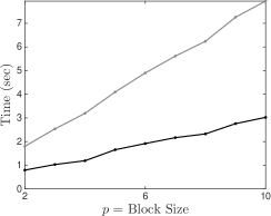
Fig. 1: Comparison of the time taken to perform $p\times 10^{5}$ matrix-vector products for the sparse sherman5 matrix for the single matrix-vector product (grey) and the block size $p$ matrix-vector product (black). Different block sizes were tested. The initial target vector was generated using Matlab’s rand() function, and the matrix simply acted upon this vector repeatedly.

In this scenario, we see that the block matrix-vector product is able to outperform the single matrix-vector product in this case, in Matlab. However, we are more interested in an iteration for iteration performance comparison of a block Krylov subspace method versus a single-vector Krylov subspace method. We pose the question, do the benefits of convergence in fewer iterations outweigh the increased number of floating-point operations of the block matrix-vector product? In Figure 2, we compare the the time taken to perform matrix-single-vector products with the time take to compute matrix-block-vector products.

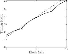
Fig. 2: In the figure on the left, we compare the time taken to perform $10^{5}$ single matrix-vector products (grey) with how much time is taken to perform the same number of block matrix-vector products for different block sizes $p$ (black). The figure on the right shows the ratio of time taken for the block matrix- vector products over the time taken for single matrix-vector products (black solid line). As predicted, the block matrix-vector product is not $p$ times as expensive. The dashed line shows the ratio if a block $p$ matrix-vector product was $\frac{2}{3}p$ times as expensive as a single matrix-vector product.

We see that, though block matrix-vector products (block size $p>1$) are more expensive to compute than the single-vector variety, they are not $p$ times as expensive.

In Figure 3, we test the code’s convergence properties as we increase the number of right-hand sides. As is predicted by the underlying theory, the increased number of right-hand sides generates a richer space from which to select our approximation updates and from which to recycle, though the marginal benefit decreases for each additional right-hand side.

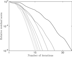
Fig. 3: Performance of block recycled GMRES GMRES with $m=100$ and $k=50$ on the sherman5 matrix from Matrix Market [16] preconditioned with ILU(0)as we increase the number of right-hand sides. The first right-hand side is packaged with the matrix. The other right-hand sides are generated using Matlab’s rand() function. Convergence is measured by computing the residual norm associated to the first right-hand side. Lightness of the convergence curves increases as we add more right-hand sides. The darkest curve is for the case $p=1$ and the lightest curve is for the case $p=10$.

We extracted matrices from seven consecutive iterations of a Tramonto Newton iteration from the POLY1_CMS_1D test problem [3]. For each iteration, we precondition using ILU(0). We compare the performance of GMRES, block GMRES with 3 right-hand sides, Recycled GMRES  and our block Recycled GMRES algorithm on all 7 systems. In the case of the block methods, one right-hand side generated by the Tramonto package, and the other two right-hand sides were random, generated using Matlab’s rand(). In the case of these Newton iterations for these relatively small systems (dimension $\approx~{}14000$), convergence for the preconditioned system is quick enough that we are able to recycle the entire Krylov subspace when running Recycled GMRES and block Recycled GMRES for the first few systems in the sequence for properly chosen recycled subspace dimension.

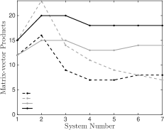
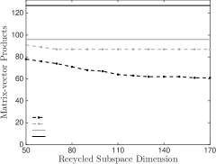
Fig. 4: In the left-hand figure, we see the matrix-vector product count for block recycled GMRES solving linear systems involving the Jacobian for 7 sequential Newton Steps of fluid DFT problem from Tramonto software package. ILU(0) preconditioning was used. The figure on the right shows the total matrix-vector product count for various recycle space dimensions Effectively, as we move to the right in this figure, we reach a point at which no recycled subspace information is ever discarded in the experiment.

In Figure 4, we plot the number of matrix-vector products needed to solve each system. Observe that for both algorithms, recycling greatly reduces the number of matrix-vector products needed to solve later systems. Furthermore, we get a per-system reduction when moving from Recycled GMRES to block Recycled GMRES  particularly for systems appearing early in the sequence. In Figure 4, the benefit of the block method is most pronounced for the first system. This suggests that for some problems, we may gain the most benefit by applying block Recycled GMRES only for the first system. This will yield a high-quality recycled subspace, and we apply single-vector Recycled GMRES for the rest of the systems. We also see that, for large enough recycled subspace, we achieve a 30% reduction in overall matrix-vector products when moving from single right-hand side Recycled GMRES to block Recycled GMRES with two random right-hand sides.

Table 1: Fifteen different matrices downloaded from the University of Florida Sparse Matrix Library [16] with various sparsity patterns. The matrix qcdRealPart is the real part of the matrix conf5-0-4x4-10 from [16]

Name	Dimension	# Non-zeros	Sparsity
Freescale1	$3428755$	$17052626$	$0.0001\%$
CoupCons3D	$416800$	$17277420$	$0.0099\%$
rajat31	$4690002$	$20316253$	$0.0001\%$
FullChip	$2987012$	$26621983$	$0.0003\%$
cage14	$1505785$	$27130349$	$0.0012\%$
RM07R	$381689$	$37464962$	$0.0257\%$
epb3	$84617$	$463625$	$0.0065\%$
qcdRealPart	$49152$	$1916928$	$0.0793\%$
crashbasis	$160000$	$1750416$	$0.0068\%$
Hamrle3	$1447360$	$5514242$	$0.0003\%$
HV15R	$2017169$	$283073458$	$0.0070\%$
lung2	$160000$	$1750416$	$0.0068\%$
ML_Geer	$1504002$	$110686677$	$0.0049\%$
pre2	$659033$	$5834044$	$0.0013\%$
twotone	$120750$	$1206265$	$0.0083\%$

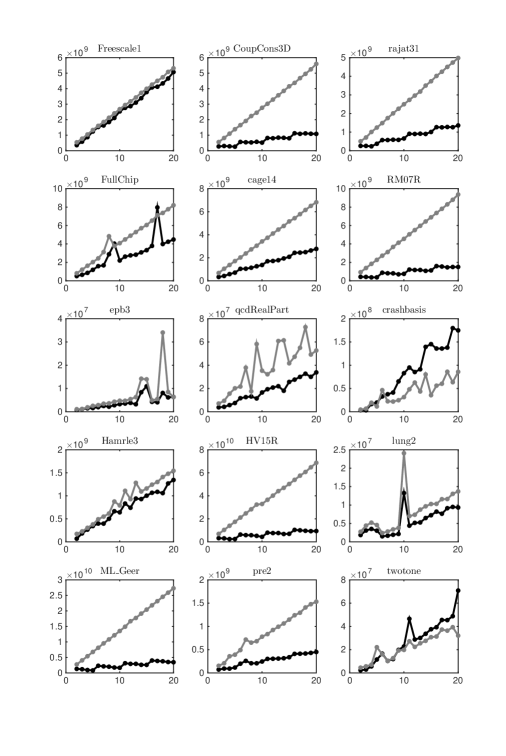
\begin{picture}(0.0,0.0)\end{picture}

Fig. 5: For the fifteen different matrices from Table 1, a comparison of cache misses for the matrix applied to different sizes of vector blocks both all-at-once (black lines) and one-at-a-time (gray lines). The horizontal axes show block size and the vertical axes show number of cache misses per 100 executions of the experiment.

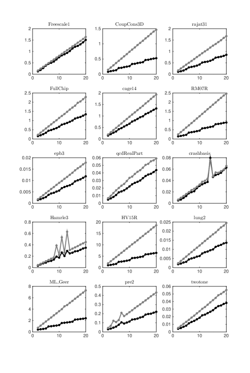
\begin{picture}(0.0,0.0)\end{picture}

Fig. 6: For the fifteen different matrices from Table 1, a comparison average timings (in seconds) for the projected matrix applied to different sizes of vector blocks both all-at-once (black lines) and one-at-a-time (gray lines). The horizontal axes show block size and the vertical axes show the average time in seconds required for each experiment.

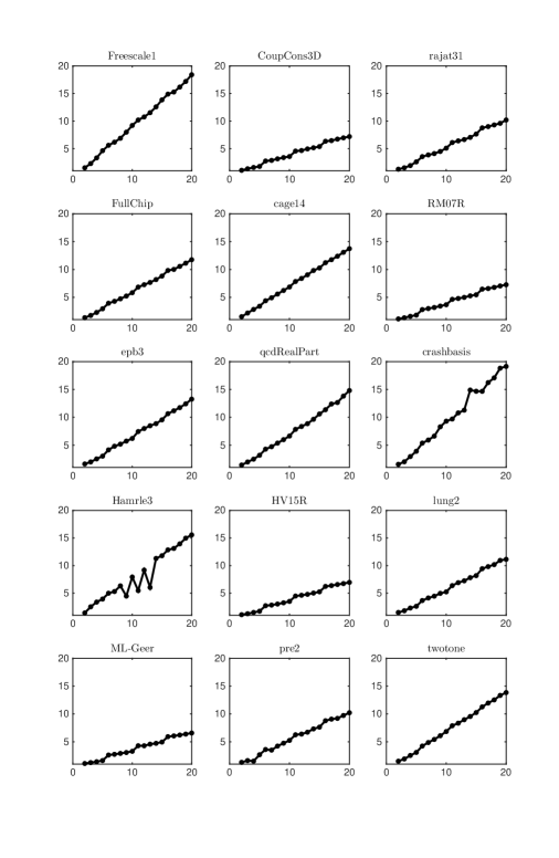
\begin{picture}(0.0,0.0)\end{picture}

Fig. 7: For the fifteen different matrices from [16], the ratio of the average time taken to apply the matrix to different sizes of vector blocks versus to a single vector. The horizontal axes show block size and the vertical axes show the ratio for each block.

6.2 Data movement experiments

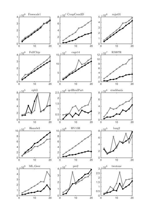
\begin{picture}(0.0,0.0)\end{picture}

Fig. 8: For the fifteen different matrices from Table 1, a comparison of cache misses for the projected matrix $(\mathbf{I}-\mathbf{C}\mathbf{C}^{\ast})\mathbf{A}$ applied to different sizes of vector blocks both all-at-once (black lines) and one-at-a-time (gray lines). The projector was applied using a modified Gram-Schmidt algorithm, and $\mathbf{C}\in\mathbb{R}^{n\times 100}$. The horizontal axes show block size and the vertical axes show number of cache misses per 100 executions of the experiment.

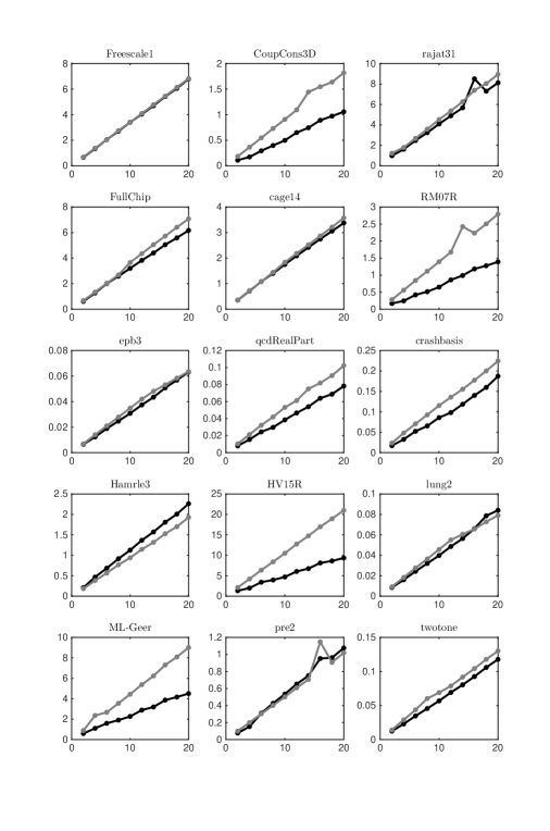
\begin{picture}(0.0,0.0)\end{picture}

Fig. 9: For the fifteen different matrices from [16], a comparison average timings (in seconds) for the projected matrix $(\mathbf{I}-\mathbf{C}\mathbf{C}^{\ast})\mathbf{A}$ applied to different sizes of vector blocks both all-at-once (black lines) and one-at-a-time (gray lines). The projector was applied using a modified Gram-Schmidt algorithm, and $\mathbf{C}\in\mathbb{R}^{n\times 100}$. The horizontal axes show block size and the vertical axes show the average time in seconds required for each experiment.

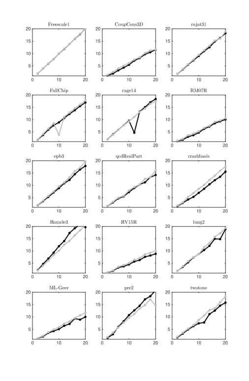
\begin{picture}(0.0,0.0)\end{picture}

Fig. 10: For the fifteen different matrices from [16], the ratio of the average time taken to apply the matrix to different sizes of vector blocks versus to a single vector for the projected operator $\left(\mathbf{I}-\mathbf{C}\mathbf{C}^{\ast}\right)\mathbf{A}$. The projector is applied using either a modified Gram-Schmidt algorithm (black line) or multiple passes of classical Gram-Schmidt (gray line), and $\mathbf{C}\in\mathbb{R}^{n\times 100}$. The horizontal axes show block size and the vertical axes show the ratio for each block size.

In this section, we run a variety of performance tests on matrices of various sparsity patterns and levels coming both from real applications [16] and from test sets we artificially constructed. The tests were performed on a shared memory machine with 8 Intel Xeon E7-4870 2.4Ghz processors, each with 10 cores (i.e., a total of 80 CPU cores) and a total of 1 terabyte main memory. Each processor has 30 megabytes of L3 cache (3 megabytes per core). Experiments were run in serial. Using compiled Trilinos codes [2], we compare performance of large sparse operators being applied to blocks of vectors of varying block sizes. For each matrix $\mathbf{A}$, we compare multiplying the matrix times the entire block versus multiplying the matrix times each vector individually. For each matrix, the experiment is repeated for the projected operator $\left(\mathbf{I}-\mathbf{C}\mathbf{C}^{\ast}\right)\mathbf{A}$ for subspaces ${\mathcal{U}}$ of different dimensions. Before each test was performed, a block matrix-vector product was executed so that any prefetching of data into the cache would occur before the start of the test and thus not interfering with our measurements.

Performance is measured in multiple ways. First, each experiment is performed $100$ times and the average time in seconds for those experiments is taken. Second, we compiled the Intel Performance Counter Monitor (PCM) libraries [1] and inserted appropriate function calls into our test code, and these were used to take measurements directly from the processor for each experiment. Namely, the PCM allows one to measure bytes read by the processor, the percentage of cache hits, and the number of cache misses occurring during the experiment. A cache hit refers to the instance that a wanted piece of data is already stored in cache on the processor, increasing the speed of access. A cache miss is when a wanted piece of data is not on the cache and thus must be accessed from main memory, causing a delay due to data movement needs. In our experiments, we demonstrate that often, the sparse matrix times a dense block of vectors has superior performance when measured in these cache- and data- related metrics over the sparse matrix-vector product.

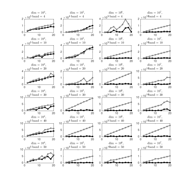
\begin{picture}(0.0,0.0)\end{picture}

Fig. 11: For banded matrices of different dimensions, a comparison cache misses for the matrix applied to different sizes of vector blocks both all-at-once (black lines) and one-at-a-time (gray lines). The horizontal axes show block size and the vertical axes show number of cache misses per 100 executions of the experiment.

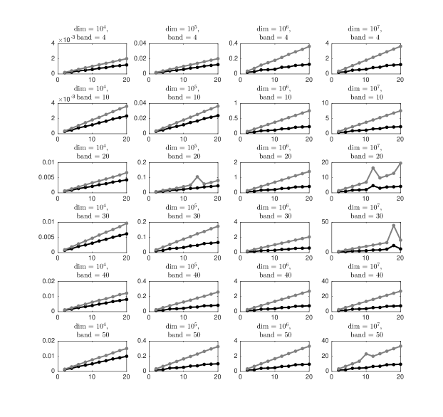
\begin{picture}(0.0,0.0)\end{picture}

Fig. 12: For banded matrices of different dimensions, a comparison average timings (in seconds) for the projected matrix applied to different sizes of vector blocks both all-at-once (black lines) and one-at-a-time (gray lines). The horizontal axes show block size and the vertical axes show the average time in seconds required for each experiment.

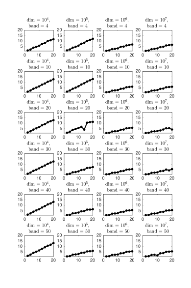
\begin{picture}(0.0,0.0)\end{picture}

Fig. 13: For banded matrices of different dimensions, the ratio of the average time taken to apply the matrix to different sizes of vector blocks versus to a single vector. The horizontal axes show block size and the vertical axes show the ratio for each block.

In our first set of experiments, we take measurements for fifteen sample matrices arising in a variety of applications, downloaded from [16]. We begin by taking measurements for just the application of the matrix to various sizes of block vectors. In Table 1, names and relevant characteristics of the matrices are shown. In Figure 5, comparisons of cache misses for single- and block-matvecs are shown for block sizes between $2$ and $20$. In Figure 6, average timings are shown for the same experiments. In Figure 7, we compare the ratio of the time take to multiply the matrix times a block of vectors to the time taken to multiply times just one vector. This demonstrates that it is often the case that multiplying times $L$ vectors is not $L$-times as expensive as multiplying times a single vector. In these experiments, we see the greatest computational benefit for larger matrices, which is when a matvec becomes an I/O-bound operation, i.e., the rate at which data is used is faster than the rate at which it is retrieved. If one compares the matrix sizes from Table 1 against the data in Figures 5–7, one sees that the greatest performance difference in the two experiments is for the matrices with the largest number of nonzeros (ML_Geer, CoupCons3D, etc.). For small matrices (e.g., epb3) one observes hardly any difference. This confirms that using block operations would likely only provides benefit for large matrices. We note that we can transfer these results to the parallel setting, where we instead consider the situation that the part of the matrix stored on a specific node is large with respect to the L3 cache size. Note that Figure 11 illustrates this relationship; the figures further down and to the right show increasingly larger differences in cache misses between the two experiments.

We then took the same measurements but for the projected operator $\left(\mathbf{I}-\mathbf{P}\right)\mathbf{A}$. We show below experiments for the case that $\dim{\mathcal{C}}=10$. We also performed the same experiments for $\dim{\mathcal{C}}=50$ and $\dim{\mathcal{C}}=100$, but the results were not substantially different from those shown. We see in all three experiments that the cache efficiencies observed for applying the matrix to blocks of vectors is diminished when a projector is composed with the operator. In Figures 8 and 9, we see that for many matrices, there is similar performance, in terms of timings and numbers of cache misses, whether the matrix is applied to the full block or to each vector in the block individually. In some cases, one-at-a-time application is actually superior. We also again show the ratio between time taken to multiply the projected matrix times a block of vectors versus multiplying times just one vector. In this experiment, we investigated whether there was much difference whether one uses modified Gram-Schmidt or multiple passes of classical Gram-Schmidt (DGKS) [14].

This experience is important when considering the performance of a block recycled GMRES method as compared to standard block GMRES. The cache-efficiency benefits of block methods does not always extend to the orthogonalization routines tested in this paper. Thus it may be more appropriate to compare the performance of block GMRES and recycled block GMRES for total search space dimension being approximately the same, so that the number of orthogonalization is equivalent for both methods.

In our second set of experiments, we repeat the same tests but for some large, sparse, banded matrices. These were constructed in Matlab using rand() and spdiags() . We constructed matrices with dimensions of $10^{4}$, $10^{5}$, $10^{6}$, and $10^{7}$. The matrices with banded sizes of $4$, $10$, $20$, $30$, $40$, and $50$ were constructed. Block sizes tested were the even integers in the interval $\left[2,20\right]$. As the previous experiments demonstrated that there is a great loss of cache efficiency when applying the projected operator, we restrict these experiments to the case of the unprojected operator. In Figure 11, we compare the number of cache misses encountered when applying the matrices to a block of vector at once versus to the same block one column at-a-time. In Figure 12 we compare average timings for the same two cases. In Figure 13, we calculate the ratio between the average time taking to apply each operator to a block of vectors versus applying it to a single vector. This to a large extent indicates how much more expensive an iteration (dominated by the cost of the matrix-vector product) will be for a block method versus the single-vector version of that method. We see again for these artificially constructed sparse matrices that we benefit from data movement efficiency for block methods. Furthermore, because the structures of these matrices is precisely known, it is easier to compare results for different matrices in this group.

7 Discussion and conclusions

We chose to restrict the experiments in Section 6.2 to the matrix-vector product. We focus on the performance of the application of $\mathbf{A}$ and of $(\mathbf{I}-\mathbf{P})$ as they are two of the most dominant costs in Algorithm 4.1. Many of the other operations are dense matrix-matrix operations with already confirmed cache efficiency characteristics. In particular, we use the Householder transformation block storage and application strategy of Gutknecht and Schmelzer [27] which means application of the previous Householder transformations is also a matrix-matrix operation. Thus the experiments presented in Section 6.2 are analogous to per iteration costs of our method, and for the unprojected operator any block method; see, e.g., [9].

A C++ implementation of Algorithm 4.1 is available as a part of the Belos package of Trilinos [47], and a Matlab implementation is available at [48]. Furthermore, as we have only shown a small subset of the data coming from our performance results, we also provide tables containing the full, raw performance results as a supplement to this paper.

References

-
[1]
Intel performance counter monitor.
Accessed on 28 February, 2016 at http:
www.intel.com/software/pcm. -
[2]
The Trilinos Project website., Accessed December 10, 2014.
http://trilinos.org/. -
[3]
Description of the poly1-cms-1d problems, Accessed February 24, 2012.
https://software.sandia.gov/tramonto/src_docs/POLY1__CMS__1D_2README.html. - [4] Abdou M. Abdel-Rehim, Ronald B. Morgan, Dywayne A. Nicely, and Walter Wilcox, Deflated and restarted symmetric Lanczos methods for eigenvalues and linear equations with multiple right-hand sides, SIAM Journal on Scientific Computing, 32 (2010), pp. 129–149.
- [5] E. Agullo, L. Giraud, and Y.-F. Jing, Block GMRES method with inexact breakdowns and deflated restarting, SIAM Journal on Matrix Analysis and Applications, 35 (2014), pp. 1625–1651.
- [6] Kapil Ahuja, Michael L. Parks, Eric T. Phipps, Andy G. Salinger, and Eric de Sturler, Krylov recycling for climate modeling and uncertainty quantification, Tech. Report SAND2010-8783P, Sandia National Laboratories Computer Science Research Institute, 2010.
- [7] James Baglama and Lothar Reichel, Augmented GMRES-type methods, Numerical Linear Algebra with Applications, 14 (2007), pp. 337–350.
- [8] , Decomposition methods for large linear discrete ill-posed problems, Journal of Computational and Applied Mathematics, 198 (2007), pp. 332–343.
- [9] Allison H. Baker, John M. Dennis, and Elisabeth R. Jessup, On improving linear solver performance: a block variant of GMRES, SIAM Journal on Scientific Computing, 27 (2006), pp. 1608–1626.
- [10] Allison H. Baker, Elizabeth R. Jessup, and Thomas Manteuffel, A technique for accelerating the convergence of restarted GMRES, SIAM Journal on Matrix Analysis and Applications, 26 (2005), pp. 962–984.
- [11] Stephen L. Campbell, Ilse C. F. Ipsen, C. Tim Kelley, and Carl D. Meyer, GMRES and the minimal polynomial, BIT, 36 (1996), pp. 664–675.
- [12] K. Carlberg, V. Forstall, and R. Tuminaro, Krylov-subspace recycling via the POD-augmented conjugate-gradient method, ArXiv e-prints, (2015).
- [13] Anthony T. Chronopoulos and Andrey B. Kucherov, Block--step Krylov iterative methods, Numerical Linear Algebra with Applications, 17 (2010), pp. 3–15.
- [14] J. W. Daniel, W. B. Gragg, L. Kaufman, and G. W. Stewart, Reorthogonalization and stable algorithms for updating the Gram-Schmidt factorization, Math. Comp., 30 (1976), pp. 772–795.
- [15] Dean Darnell, Ronald B. Morgan, and Walter Wilcox, Deflated GMRES for systems with multiple shifts and multiple right-hand sides, Linear Algebra and its Applications, 429 (2008), pp. 2415–2434.
- [16] Timothy A. Davis and Yifan Hu, The University of Florida sparse matrix collection, ACM Transactions in Mathematical Software, 38 (2011), pp. 1:1–1:25.
- [17] Eric de Sturler, Nested Krylov methods based on GCR, Journal of Computational and Applied Mathematics, 67 (1996), pp. 15–41.
- [18] , Truncation strategies for optimal Krylov subspace methods, SIAM Journal on Numerical Analysis, 36 (1999), pp. 864–889.
- [19] Yiqiu Dong, Henrik Garde, and Per Christian Hansen, R3GMRES: including prior information in GMRES-type methods for discrete inverse problems, Electron. Trans. Numer. Anal., 42 (2014), pp. 136–146.
- [20] Michael Eiermann, Oliver G. Ernst, and Olaf Schneider, Analysis of acceleration strategies for restarted minimal residual methods, Journal of Computational and Applied Mathematics, 123 (2000), pp. 261–292.
- [21] Roland W. Freund, Quasi-kernel polynomials and their use in non-Hermitian matrix iterations, Journal of Computational and Applied Mathematics, 43 (1992), pp. 135–158.
- [22] Kyle A. Gallivan, Michael T. Heath, Esmond Ng, James M. Ortega, Barry W. Peyton, Robert J. Plemmons, Charles H. Romine, Ahmed H. Sameh, and Robert G. Voigt, Parallel Algorithms for Matrix Computations, Society for Industrial and Applied Mathematics, 1990.
- [23] André Gaul, Recycling Krylov subspace methods for sequences of linear systems: Analysis and applications, PhD thesis, Technischen Universität Berlin, 2014.
- [24] André Gaul, Martin H. Gutknecht, Jörg Liesen, and Reinhard Nabben, A framework for deflated and augmented Krylov subspace methods, SIAM Journal on Matrix Analysis and Applications, 34 (2013), pp. 495–518.
- [25] André Gaul and Nico Schlömer, Preconditioned recycling Krylov subspace methods for self-adjoint problems, Electronic Transactions on Numerical Analysis, 44 (2015), pp. 522–547.
- [26] Martin H. Gutknecht, Block Krylov space methods for linear systems with multiple right-hand sides: an introduction, in Modern Mathematical Models, Methods and Algorithms for Real World Systems, Abul Hasan Siddiqi, Iain S. Duff, and Ole Christensen, eds., New Delhi, 2007, Anamaya Publishers, pp. 420–447.
- [27] Martin H. Gutknecht and Thomas Schmelzer, Updating the QR decomposition of block tridiagonal and block Hessenberg matrices, Applied Numerical Mathematics, 58 (2008), pp. 871–883.
- [28] Michael A. Heroux, Andrew G. Salinger, and Laura J. D. Frink, Parallel segregated Schur complement methods for fluid density functional theories, SIAM Journal on Scientific Computing, 29 (2007), pp. 2059–2077.
- [29] Mark Hoemmen, Communication-avoiding Krylov subspace methods, PhD thesis, University of California Berkeley, 2010.
- [30] Chao Jin and Xiao-Chuan Cai, A preconditioned recycling gmres solver for stochastic helmholtz problems, Communications in Computational Physics, 6 (2009), p. 342.
- [31] Chao Jin, Xiao-Chuan Cai, and Congming Li, Parallel domain decomposition methods for stochastic elliptic equations, SIAM Journal on Scientific Computing, 29 (2007), pp. 2096–2114.
- [32] Yan-Fei Jing, Luc Giraud, Bruno Carpentieri, and Ting-Zhu Huang, Recycling block flexible GMRES method with inexact breakdowns for sequences of multiple right-hand side linear systems, In Preparation, (2016).
- [33] Misha E. Kilmer and Eric de Sturler, Recycling subspace information for diffuse optical tomography, SIAM Journal on Scientific Computing, 27 (2006), pp. 2140–2166.
- [34] Richard B. Lehoucq and Danny C. Sorensen, Deflation techniques for an implicitly restarted Arnoldi iteration, SIAM Journal on Matrix Analysis and Applications, 17 (1996), pp. 789–821.
- [35] Jing Meng, Pei-Yong Zhu, and Hou-Biao Li, A block GCROT(m,k) method for linear systems with multiple right-hand sides, Journal of Computational and Applied Mathematics, 255 (2014), pp. 544–554.
- [36] Marghoob Mohiyuddin, Mark Hoemmen, James Demmel, and Katherine Yelick, Minimizing communication in sparse matrix solvers, in Proceedings of the Conference on High Performance Computing Networking, Storage and Analysis, SC ’09, New York, NY, USA, 2009, ACM, pp. 36:1–36:12.
- [37] Ronald B. Morgan, Computing interior eigenvalues of large matrices, Linear Algebra and its Applications, 154/156 (1991), pp. 289–309.
- [38] , A restarted GMRES method augmented with eigenvectors, SIAM Journal on Matrix Analysis and Applications, 16 (1995), pp. 1154–1171.
- [39] , Implicitly restarted GMRES and Arnoldi methods for nonsymmetric systems of equations, SIAM Journal on Matrix Analysis and Applications, 21 (2000), pp. 1112–1135.
- [40] , GMRES with deflated restarting, SIAM Journal on Scientific Computing, 24 (2002), pp. 20–37.
- [41] Ronald B. Morgan and Min Zeng, Harmonic projection methods for large non-symmetric eigenvalue problems, Numerical Linear Algebra with Applications, 5 (1998), pp. 33–55.
- [42] Keiichi Morikuni, Lothar Reichel, and Ken Hayami, FGMRES for linear discrete ill-posed problems, Applied Numerical Mathematics, 75 (2014), pp. 175–187.
- [43] Dianne P. O’Leary, The block conjugate gradient algorithm and related methods, Linear Algebra and its Applications, 29 (1980), pp. 293–322.
- [44] , Parallel implementation of the block conjugate gradient algorithm, Parallel Computing. Theory and Applications, 5 (1987), pp. 127–139.
-
[45]
Michael Parks, Sandia National Laboratories professional
website: Software page, 2011.
Available at
http://www.sandia.gov/~mlparks/software.html. - [46] Michael L. Parks, Eric de Sturler, Greg Mackey, Duane D. Johnson, and Spandan Maiti, Recycling Krylov subspaces for sequences of linear systems, SIAM Journal on Scientific Computing, 28 (2006), pp. 1651–1674.
- [47] Michael L. Parks and Kirk M. Soodhalter, Block GCRO-DR. in Belos package of the Trilinos C++ Library, 2011.
-
[48]
Michael L. Parks, Kirk M. Soodhalter, and Daniel B. Szyld, Block
GCRO-DR: A version of the recycled GMRES method using block Krylov subspaces
and harmonic Ritz vectors, Apr. 2016.
Available at
http://dx.doi.org/10.5281/zenodo.48836. - [49] Axel Ruhe, Implementation aspects of band Lanczos algorithms for computation of eigenvalues of large sparse symmetric matrices, Mathematics of Computation, 33 (1979), pp. 680–687.
- [50] Yousef Saad, A flexible inner-outer preconditioned GMRES algorithm, SIAM Journal on Scientific Computing, 14 (1993), pp. 461–469.
- [51] , Analysis of augmented Krylov subspace methods, SIAM Journal on Matrix Analysis and Applications, 18 (1997), pp. 435–449.
- [52] , Iterative Methods for Sparse Linear Systems, SIAM, Philadelphia, Second ed., 2003.
- [53] Yousef Saad and Martin H. Schultz, GMRES: A generalized minimal residual algorithm for solving nonsymmetric linear systems, SIAM Journal on Scientific and Statistical Computing, 7 (1986), pp. 856–869.
- [54] Valeria Simoncini and Efstratios Gallopoulos, Convergence properties of block GMRES and matrix polynomials, Linear Algebra and its Applications, 247 (1996), pp. 97–119.
- [55] Valeria Simoncini and Daniel B. Szyld, The effect of non-optimal bases on the convergence of Krylov subspace methods, Numerische Mathematik, 100 (2005), pp. 711–733.
- [56] , On the occurrence of superlinear convergence of exact and inexact Krylov subspace methods, SIAM Review, 47 (2005), pp. 247–272.
- [57] , Recent computational developments in Krylov subspace methods for linear systems, Numerical Linear Algebra with Applications, 14 (2007), pp. 1–59.
- [58] Kirk M. Soodhalter, A block MINRES algorithm based on the banded Lanczos method, Numerical Algorithms, 69 (2015), pp. 473–494.
- [59] Henk A. van der Vorst and Kees Vuik, The superlinear convergence behaviour of GMRES, Journal of Computational and Applied Mathematics, 48 (1993), pp. 327–341.
- [60] Brigitte Vital, Etude de quelques méthodes de résolution de problèmes linéaires de grande taille sur multiprocesseur, PhD thesis, Université de Rennes, 1990.
- [61] Shun Wang, Eric de Sturler, and Glaucio H. Paulino, Large-scale topology optimization using preconditioned Krylov subspace methods with recycling, International Journal for Numerical Methods in Engineering, 69 (2007), pp. 2441–2468.