The adaptive-loop-gain adaptive-scale CLEAN deconvolution of radio interferometric images

Abstract

CLEAN algorithms are a class of deconvolution solvers which are widely used to remove the effect of the telescope Point Spread Function (PSF). Loop gain is one important parameter in CLEAN algorithms. Currently the parameter is fixed during deconvolution, which restricts the performance of CLEAN algorithms. In this paper, we propose a new deconvolution algorithm with an adaptive loop gain scheme, which is referred to as the adaptive-loop-gain adaptive-scale CLEAN (Algas-Clean) algorithm. The test results show that the new algorithm can give a more accurate model with faster convergence.

Keywords methods: data analysis; techniques: image processing

1 Introduction

Aperture synthesis technique breaks through the limitation of resolution of a single antenna physical aperture. Such telescopes however do not measure all the spatial frequencies, leading to a Point Spread Function (PSF) with wide-spread sidelobes. The PSF limits the imaging dynamic range to only a few 100:1.

There are many methods to remove the effects of the PSF, e.g. CLEAN algorithms (Högbom, 1974; Clark, 1980; Schwab & Cotton, 1983; Bhatnagar & Cornwell, 2004; Cornwell, 2008; Rau & Cornwell, 2011), Maximum Entropy Methods (MEM) (Cornwell & Evans, 1985; Narayan & Nityananda, 1986) and compressive sensing reconstruction algorithms (Wiaux et al., 2009; Wenger et al., 2010; Li et al., 2011; Carrillo et al., 2012). The CLEAN algorithm (Högbom, 1974) and its variants model the sky brightness distribution as a set of delta functions. This however is non-optimal to model extended emission. To improve the imaging performance for extended emission, several scale-sensitive algorithms have been proposed (Bhatnagar & Cornwell, 2004; Cornwell, 2008; Rau & Cornwell, 2011). The multi-scale CLEAN algorithms (Cornwell, 2008; Rau & Cornwell, 2011) use tapered paraboloids to decompose sky sources by a matched-filtering technique. Better representation for extended sources makes the multi-scale CLEAN algorithms be able to use a larger loop gain, e.g. $0.5$ or even larger (Cornwell, 2008). However it uses a fixed set of components, the size of which cannot be varied. The adaptive scale pixel decomposition deconvolution (Asp-Clean) algorithm (Bhatnagar & Cornwell, 2004) uses an optimization technique to overcome this problem by keeping the size and location of the components variable. All these algorithms use the loop gain parameter which controls the feed-back of the model in computing the residuals at each iteration. The value of the loop gain therefore strongly impacts both the imaging performance and rate of convergence. The value of loop gain is fixed, which limits the performance of these algorithms. In this paper therefore, we propose an adaptive loop gain scheme to improve the fidelity of model and convergence speed of the Asp-Clean algorithm.

In section 2, we recap CLEAN algorithms. In section 3, we describe the motivation of developing an adaptive loop gain scheme. In section 4, we describe the details of the Algas-Clean algorithm. In section 5, some examples are provided to show the performance of the Algas-Clean algorithm. In section 6, we summary this work.

2 CLEAN algorithms

Interferometric measurement is in spatial frequency domain,

$$\bm{V}^{measured}=\bm{S}\left(\bm{F}\bm{I}^{true}+\bm{n}_{0}\right),$$ (1)

where $\bm{V}^{measured}$ is the measured visibility data, $\bm{S}$ is the sampling function which encodes the missing spatial frequency information, $\bm{F}$ is the Fourier transformation, $\bm{I}^{true}$ is the true sky image and $\bm{n}_{0}$ is the random noise in the visibility domain (Thompson et al., 2001). In the image plane, the above equation is

$$\bm{I}^{dirty}=\bm{B}\ast\bm{I}^{true}+\bm{n},$$ (2)

where $\bm{I}^{dirty}$ is the dirty image which is the inverse Fourier transformation of $\bm{V}^{measured}$, $\bm{B}$ is the dirty beam which is the inverse Fourier transformation of $\bm{S}$, the symbol $\ast$ denotes the convolution, and $\bm{n}$ is the measurement noise.

Various deconvolution algorithms exist to remove the effects of $\bm{B}$ from $\bm{I}^{dirty}$. Deconvolution algorithms are fundamentally iterative and all modern CLEAN deconvolution algorithms have the general structure of two iterative cycles called “major cycle” and “minor cycle” (Clark, 1980; Rau et al., 2009). The major cycle involves computation of the residual image at each iteration while the minor cycle involves deconvolution of $\bm{B}$ (or it’s approximation) from the residual image at each iteration. Scale-insensitive CLEAN algorithms parameterize the sky image as a set of delta functions. The components are estimated by finding the brightest peak from the current residual image and scaling the peak with a fixed loop gain, $g$. Empirically, $g$ is typically in the range of $0.01\sim 0.25$ (Taylor et al., 1999). Scale-sensitive algorithms like Asp-Clean and MS-Clean parameterize the sky image with scale basis functions. The main difference is that the Asp-Clean algorithm parameterizes the sky brightness function with a continuous set of scales while the MS-Clean algorithm uses several discrete scales. These scale basis functions represent the extended structures much better than delta functions. However, since the components cannot always accurately model the complex extended emission, loop gain is still needed in these algorithms. Existing implementations use a fixed loop gain.

3 The motivation for an adaptive scheme for loop gains

In scale-sensitive CLEAN algorithms, a component is calculated as a scale basis function from the region with the highest total power in the current residual image. A fixed loop gain, which scales the component before subtraction, may be proper for some components but not for others. What’s more, a fixed loop gain gives each pixel of the extended component equal loop gains in the Asp-Clean and MS-Clean algorithms. This means that strong brightness and weak brightness in an extended component which are estimated from the current residual image are deemed to have same significance/reliability. This will be a problem when a tailed function like Gaussian is used, like in the Asp-Clean algorithm, to approximate a finite-support extended structure. Variable loop gain for strong brightness and weak brightness can be a better strategy. In this paper, we propose an scheme for adaptive loop gains. The basic idea is that stronger brightness owns larger loop gains than weaker brightness in an extended component. Obviously, the adaptive loop gains are shape-dependent. This can solve the problem just mentioned. From lots of tests, we found that the largest remaining errors in an image model are in the strongest brightness region. The over-estimation of the strong brightness leads to this problem. This problem can be solved by suppressing the strong part of each component. To sum up, we want to relatively suppress the strongest and weakest parts of an initial component (before subtraction) to solve the two problems mentioned above.

4 The adaptive-loop-gain adaptive-scale CLEAN algorithm

As mentioned above, the Algas-Clean algorithm is a variant of the Asp-Clean algorithm with the proposed adaptive loop gain scheme used in the minor cycle.

The Asp-Clean algorithm represents images as a set of truncated Gaussian functions,

$$\bm{I}^{model}=\sum_{i=1}^{N}g\bm{I}_{i}^{comp}\left(scale\right),$$ (3)

where $\bm{I}^{model}$ is the model composed of $N$ components, $g$ is the fixed loop gain which is used for all components, and $I_{i}^{comp}\left(scale\right)$ is the $i$th component which is a truncated Gaussian function. The Gaussian components are found by an optimization method like Levenberg-Marquardt method (Marquardt, 1963) which minimizes the objective function $\chi^{2}$,

$$\chi^{2}=\|\bm{I}_{i}^{residual}-\bm{B}\ast\bm{I}_{i}^{comp}\|_{2}^{2},$$ (4)

where $\bm{I}_{i}^{residual}$ is the residual image in $i$th iteration, and $\|\,\,\|_{2}$ is the $l2$ norm. The optimization method makes components much better match to source structures and so the Asp-Clean algorithm gives better imaging performance compared to other algorithms. But local and specific structures are almost always non-Gaussians, and in fact not fitted exactly by any function in general. The fixed loop gain is not optimal for an extended component, especially for the two problems mentioned in section 3 and can lead to an improper approximation of components. The resulting error is difficult to be corrected completely. With the proposed adaptive loop gain scheme, the approximated model is expressed as follows,

$$\bm{I}^{model}=\sum_{i=1}^{N}\bm{g}_{i}\bm{I}_{i}^{comp},$$ (5)

where $\bm{g}_{i}$ is a matrix whose elements are proportional to each pixel amplitude of the $i$th component.

A fixed loop gain equally treats strong brightness and weak brightness. This often leads to an over-estimation for weak brightness in finite-support case. In the Algas-Clean algorithm, each Gaussian component will be scaled with adaptive loop gains. It can effectively control the over-estimation of weak brightness in finite-support structures. To reduce the computational complexity, previous components will be not re-optimized in later iterations in the Algas-Clean algorithm as well as in the Asp-Clean algorithm implemented in this paper. Deconvolution is terminated when the standard deviation of residual image is less than that of noise included in the dirty image.

In this paper, we use the following method to calculate the adaptive loop gains,

$$g\left(x\right)=\sqrt{\left|a\left(1-f\left(x\right)\right)+bf\left(x\right)\right|},$$ (6)

where

$$f\left(x\right)=\frac{x-C_{min}}{C_{max}-C_{min}},$$ (7)

where the $g\left(x\right)$ is the adaptive loop gain function, $x$ is an image pixel, $a$ and $b$ are the minimum and maximum values respectively after the linear transformation, $C_{min}$ and $C_{max}$ are the minimum and maximum values of the component respectively, $\sqrt{\,\,}$ is a root square operation and $|\,\,|$ is an absolute value sign. The parameters $a$ and $b$ need to be assigned by users and $a\geq 0.0$ and $b\leq 1.0$. As mentioned earlier, the largest remaining errors in an image model are in the strongest brightness region. The square root operation in the formula (6) can relatively suppress both the weakest and strongest parts of an extended component. Suppression of the strongest parts helps in reducing the residual error while suppression of the weakest parts helps in limiting the error due to the tail of the Gaussian components.

5 Numerical experiment

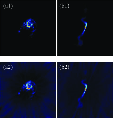
Fig. 1 : The testing data are shown here. The first and second rows are the original images and the dirty images respectively. The M31 image is shown in the first column, and the 3C31 image is shown in the second column. The brightness ranges of the two original images are from $0$ Jy/pixel to $0.1$ Jy/pixel. The brightness ranges of the dirty M31 image and the dirty 3C31 image are from $-0.040$ Jy/pixel to $0.790$ Jy/pixel and from $-0.036$ Jy/pixel to $0.839$ Jy/pixel respectively.

To show the performance of the Algas-Clean algorithm, two simulated VLA B configuration were made with the CASA software. The two test images M31 and 3C31 are used as sky models and are displayed in Fig 1. The original images are available from the NRAO’s websites . Background features in the images were removed with a threshold, the images are scaled to the brightness range from 0 Jy to 0.1 Jy and padded with zeros to make the size $512\times 512$ pixels. The total fluxes of the M31 and 3C31 images are 148.584 Jy and 88.453 Jy respectively. Gaussian noise was added to the simulated visibilities and robust weighting scheme (Briggs, 1995) (with the CASA parameters “weighting”=“briggs” and “robust”=0) used during the imaging process.

The Root of Mean Squares (RMS) of the model error image, which is the difference between the true image and the model image, is used to compare the imaging performance of reconstructions. The $RMS_{Merr}$ of a model error image is defined as

$$RMS_{Merr}=\frac{\|\bm{I}^{Merr}\|_{2}}{\sqrt{M}},$$ (8)

where $\bm{I}^{Merr}=\bm{I}^{true}-\bm{I}^{model}$ is the model error image and $M$ is the number of pixels in the model error image. Fewer and weaker structures in a model error image means that the model is closer to the underlying true image, and therefore a better reconstruction.

In the Asp-Clean algorithm, after a component is calculated by an optimization method, the component will be scaled by a loop gain for all pixels of the component. In the Algas-Clean algorithm, loop gains are adaptive for each pixel of each component. For Gaussian components, the adaptive loop gain scheme will give large loop gains to the pixels near the center of the Gaussian and small loop gains for the wing region far from the center. The wing regions of a Gaussian function make components have a very large support and therefore non-optimal to represent structures with finite support. In the Algas-Clean algorithm, the adaptive loop gain scheme will scale these values of components in the wings of the Gaussian with small loop gains. The adaptive loop gains can be truncated when they are less than a threshold. For example, a loop gain that is less than a factor of 0.001 of the maximum loop gain will be set as zero. This effectively makes Asp-Clean components tapered with better support size with the added advantage that the tapering adapts to the signal strength.

In the test, we include results from the Clark-Clean algorithm for completeness and to also motivate the fact that for modelling the extended emission, scale-sensitive algorithms like Asp-Clean give much better performance and hence we chose to optimize the Asp-Clean algorithm. A fixed loop gain of $0.1$ is used for the Clark-Clean algorithm and $0.7$ for the Asp-Clean algorithm. The adaptive loop gains of the Algas-Clean algorithm vary in the range from $0$ to $0.7$.

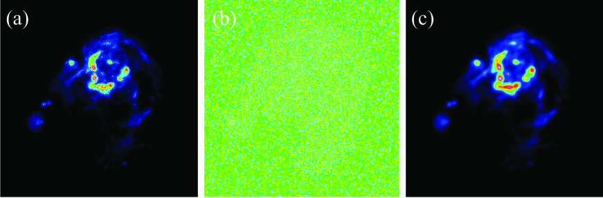
Fig. 2 : The figure shows simulated results of source M31, from the Algas-Clean algorithm. (a) The model image is displayed with the brightness range from $-0.001$ Jy/pixel to $0.103$ Jy/pixel. (b) The residual image is displayed with the brightness range from $-0.0005$ Jy/pixel to $0.0005$ Jy/pixel. The restored image is displayed with the brightness range from $-0.001$ Jy/pixel to $0.858$ Jy/pixel.

To show that as with the Asp-Clean algorithm, the Algas-Clean algorithm also models the extended emission well and fundamentally separates signal from noise leaving noise-like residuals, we show the deconvolution of the M31 images in Fig 2. The total flux of the model image in Fig 2(a) is $148.594$ Jy. The residuals are uncorrelated and noise-like implying good imaging performance of the Algas-Clean algorithm.

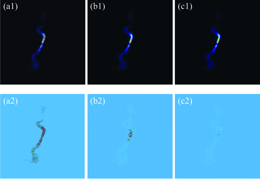
Fig. 3 : The figure shows simulated results of source M31. The first, second and third columns are from the Clark-Clean, the Asp-Clean algorithm and the Algas-Clean algorithm respectively. The model images are displayed in the first row with the brightness range from $-0.001$ Jy/pixel to $0.1$ Jy/pixel. The model error images are displayed in the second row with the brightness range from $-0.01$ Jy/pixel to $0.02$ Jy/pixel.

The test results of the 3C31 image are displayed in Fig 3. We compare the results from the widely used scale-insensitive Clark-Clean algorithm, scale-sensitive Asp-Clean algorithm and the Algas-Clean algorithm. Table 1 shows the total reconstructed fluxes of $88.253$ Jy, $88.472$ Jy and $88.481$ Jy for the Clark-Clean, the Asp-Clean algorithm and the Algas-Clean algorithm respectively. They are very close to the total flux of the true image. Comparing the results of the Clark-Clean algorithm and the Asp-Clean algorithm, we found that the scale-sensitive CLEAN algorithm has significantly improved the fidelity of model for extended sources. However, you can see that there are still lots of the remaining errors in the Asp-Clean model. The two problems mentioned earlier are the main reasons for the remaining errors in the Asp-Clean model. With the help of the proposed loop gain scheme, the Algas-Clean algorithm fundamentally solves the two problems. From Table 1, you can see that the RMS level of the remaining errors is reduced by a order of magnitude. This can also be verified by comparing Fig 3(b2) and Fig 3(c2).

Table 1 : The numerical comparison when the 3C31 residuals are in the noise level

	Gaussian	Delta	$RMS_{Merr}$	Total model flux
	components	components	(Jy/pixel)	(Jy)
Clark		$104000$	$1.584\times 10^{-3}$	$88.253$
Asp	$1400$	$48800$	$7.795\times 10^{-4}$	$88.472$
Algas	$1500$	$17200$	$7.623\times 10^{-5}$	$88.481$

From Table 1, we also see that the Algas-Clean model is composed of Gaussian components and delta functions. These compact (delta) components are from small residuals whose widths are smaller than the width of the main lobe of the dirty beam. We also can see that fewer compact components are included in the model image of the Algas-Clean algorithm indicating that Algas-Clean models the extended emission better than Asp-Clean algorithm. This means that the decomposition is more effective, and fewer number of iterations are needed in the Algas-Clean algorithm. Since the Asp-Clean algorithm is compute-intensive, fewer iterations will significantly speed it up. From our tests, we have found that the runtime of the Algas-Clean algorithm is about half the runtime of the Asp-Clean algorithm – i.e., Algas-Clean is $\sim 50$% faster than Asp-Clean with a better imaging performance. In a future paper, we will report on optimizing the fitting procedure used in Asp-Clean to further improves its run-time performance.

Because the scale-sensitive CLEAN algorithms parameterize the true image in a scale-sensitive basis, it is obvious that the proposed adaptive loop gain scheme will have the similar performance as the Algas-Clean algorithm for other scale-sensitive CLEAN algorithms.

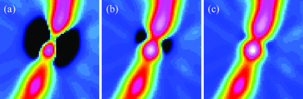
Fig. 4 : The figure shows the results of removing the first component. (a) The residual image without loop gain from the Asp-Clean algorithm. (b) The residual image with the fixed loop gain $0.7$ from the Asp-Clean algorithm. (c) The residual image with the adaptive loop gain $0\sim 0.7$ from the Algas-Clean algorithm. These images are displayed in the range from $-0.03$ Jy/pixel to $0.703$ Jy/pixel and scaling power cycles is $-2.0$.

To better illustrate the motivation of our algorithm, we use the 3C31 residual images in Fig 4 which are the residuals after removing the first component to show the effects of loop gain of 1.0, a fixed loop gain and the adaptive loop gain respectively. To display clearly, the residual images only show the region where the first component is removed. From Fig 4(a), we can see that if the component optimized by the Levenberg-Marquardt method is removed from the dirty image without a loop gain (that is, 1.0), strong negative structures appear in the residual image (as expected), due to over-subtraction. This is caused by the fact that a spatial scale function tries to represent the true sky image as much as possible by optimizing an objective function on the whole dirty image. With a fixed loop gain residual structures in Fig 4(b) are much reduced compared to the residuals in in Fig 4(a). This demonstrates that the fixed loop gain can partly suppress over-subtraction. However, the over-estimation in some parts particularly in the wings of the Gaussian component used – still exists. This reason is that when Gaussian functions are used to represent a component, a common strategy is that after getting the component, the tails are truncated at a certain ratio to the peak of the component (Bhatnagar & Cornwell, 2004; Cornwell, 2008). The method is unlikely to be optimal for all components. For example, when a Gaussian function is used to represent a flat and finite-support extended structure, the component derived by fitting a Gaussian to the structure will have extended wings beyond the extent of the true emission. Truncation alone is not good in this case and can lead to an improper truncated Gaussian, which can lead to an over-subtraction in some parts of the image. This is evident in Fig 4(b). Using the adaptive loop gain scheme smaller loop gains get used to scale-down the wings of the Gaussian component, followed by a truncation . This is more effective than the current method. It is not difficult to appreciate the effectiveness after comparing Fig 4(b) with Fig 4(c). As mentioned earlier, the other major advantage of the adaptive loop gain approach is that it not only changes across a given component, it also varies from one component to the other.

6 Summary

Since the first CLEAN algorithm was proposed in 1970s, many variants have been developed. However the fixed loop gain parameter is still used to optimize components. If we view the reconstruction problem as an approximation problem, loop gains are actually step lengths of approximation along gradient directions in an iterative algorithm. They can affect the imaging performance as well as rate of convergence significantly. In this paper, we have devised a new algorithm for a shape-dependent adaptive loop gain scheme based on amplitudes of an extended component. The adaptive loop gains are designed to solve the problems of the representation of finite-support structures and the resulting errors in the model image. Tests show that the Algas-Clean algorithm can give a more accurate model with fewer components. Fewer components also means that the approximation of the true sky image with the proposed adaptive loop gain scheme is more effective than that with fixed loop gain and also speed up deconvolution process. The work is implemented with Python and the CASA package. The script will be available soon later and the C++ implementation in the CASA package is underway.

Acknowledgements We would like to thank S. Bhatnagar and U. Rau for numerous help in this work. We thank the anonymous referee for helpful comments. This work is supported by the National Basic Research Program of China (973 program: 2012CB821804 and 2015CB857100), the National Science Foundation of China (Grant No. 11103055) and the West Light Foundation of the Chinese Academy of Sciences (Grant No. RCPY201105).

References

- Bhatnagar & Cornwell (2004) Bhatnagar, S., & Cornwell, T. J. 2004, Astron. Astrophys., 426, 747
- Briggs (1995) Briggs, D. S. 1995, Bull. Am. Astron. Soc., 27, 1444
- Carrillo et al. (2012) Carrillo, R. E., McEwen, J. D. & Wiaux 2012, Mon. Not. R. Astron. Soc., 426, 1223
- Clark (1980) Clark, B. G. 1980, Astron. Astrophys., 89, 377
- Cornwell (2008) Cornwell, T. J. 2008, EEE Journal of Selected Topics in Signal Processing, 2, 793
- Cornwell & Evans (1985) Cornwell, T. J., & Evans, K. F. 1985, Astron. Astrophys., 143, 77
- Högbom (1974) Högbom, J.A. 1974, Astron. Astrophys. Suppl. Ser., 15, 417
- Li et al. (2011) Li, F., Cornwell, T. J. & Hoog, F. de 2011, Astron. Astrophys., 31, 528
- Marquardt (1963) Marquardt, D. W. 1963, Journal of the society for industrial and Applied Mathematics, 11, 431
- Narayan & Nityananda (1986) Narayan, R. & Nityananda, R. 1986, ARA&A, 24, 127
- Rau et al. (2009) Rau, U.,Bhanagar, S., Vronkov, M.A., & Cornwell, T.J., 2009, Proc. of IEEE,97,1472
- Rau & Cornwell (2011) Rau, U., & Cornwell, T. J. 2011, Astron. Astrophys., 532, A71
- Schwab & Cotton (1983) Schwab, F. R., & Cotton, W. D. 1983, Astron. J., 88, 688
- Taylor et al. (1999) Taylor, G.B., Carilli, C.L., & Perley, R.A., 1999, synthesis imaging in radio astronomy II
- Thompson et al. (2001) Thompson, A. R.,Moran,J. M., & Swenaon, G. W. 2001,Interferometry and synthesis in radio astronomy, 2nd Edition
- Wenger et al. (2010) Wenger, S., Magnor, M., Pihlstrom, Y., Bhatnagar, S., & Rau, U. 2010, Publ. Astron. Soc. Pac., 122, 1367
- Wiaux et al. (2009) Wiaux, Y., Jacques, L., Puy, G., Scaife, A. M. M., & Vandergheynst, P. 2009, Mon. Not. R. Astron. Soc., 395, 1733