Non-Minimality
of the Width-$w$ Non-adjacent Form
in Conjunction with
Trace One $\tau$-adic Digit Expansions and
Koblitz Curves in Characteristic Two

Abstract.

This article deals with redundant digit expansions with an imaginary quadratic algebraic integer with trace $\pm 1$ as base and a minimal norm representatives digit set. For $w\geq 2$ it is shown that the width-$w$ non-adjacent form is not an optimal expansion, meaning that it does not minimize the (Hamming-)weight among all possible expansions with the same digit set. One main part of the proof uses tools from Diophantine analysis, namely the theory of linear forms in logarithms and the Baker–Davenport reduction method.

Part I The Beginning

1. Introduction

Let $\tau$ be an (imaginary quadratic) algebraic integer and $\mathcal{D}$ a finite subset of $\mathbbm{Z}[\tau]$ including zero. Choosing the digit set $\mathcal{D}$ properly, we can represent $z\in\mathbbm{Z}[\tau]$ by a finite sum

$$\sum_{\ell=0}^{L-1}\sigma_{\ell}\tau^{\ell},$$

where the digits $\sigma_{\ell}$ lie in $\mathcal{D}$. We call this representation a digit expansion of $z$. Using a redundant digit set $\mathcal{D}$, i.e., taking more digits than needed to represent all elements of $\mathbbm{Z}[\tau]$, each element can be written in different ways. Of particular interest are expansions which have the lowest number of nonzero digits. We call those expansions optimal or minimal expansions.

The motivation looking at such expansions comes from elliptic curve cryptography. There the scalar multiplication of a point on the curve is a crucial operation and has to be performed as efficiently as possible. The standard double-and-add algorithm can be extended by windowing methods, see for example [6, 8, 18, 25, 26]. Translating this into the language of digit expansions means the usage of redundant digit expansions with base $2$. However, using special elliptic curves, for example Koblitz curves, see [14, 15, 25, 26], the “expensive” doublings can be replaced by the “cheap” application of the Frobenius endomorphism over finite fields. In the world of digit expansions this means taking an imaginary quadratic algebraic integer as base. This leaves us with the additions of points of the elliptic curve as an “expensive” operation. The number of such additions is basically the number of nonzero digits in an expansion. Therefore minimizing this number is an important goal.

We are now going back to expansions with a low number of nonzero digits. Let the parameter $w\geq 2$ be an integer. Then one special expansion is the width-$w$ non-adjacent form, where in each block of width $w$ at most one digit is not equal to zero, see Reitwiesner [22] who introduced this notion for $w=2$ and others including Muir and Stinson [19] and Solinas [25, 26]. It will be abbreviated by $w$-NAF. This expansion contains, by construction, only few nonzero digits. When we use a digit set consisting of zero and of representatives with minimal norm of the residue classes modulo $\tau^{w}$ excluding those which are divisible by $\tau$, then the $w$-NAF-expansion is optimal (minimal) in a lot of cases. For example, using an integer (absolute value at least $2$) as base $\tau$, the $w$-NAF is a minimal/optimal expansion, see Reitwiesner [22], Jedwab and Mitchell [13], Gordon [8], Avanzi [1], Muir and Stinson [19], and Phillips and Burgess [21]. As a digit set it contains in these cases zero and all integers with absolute value smaller than $\frac{1}{2}\left\lvert{\tau}\right\rvert^{w}$ and not divisible by $\tau$.

A general criterion for optimality of the $w$-NAF-expanions can be found in Heuberger and Krenn [12]: The $w$-NAF of each element is optimal, if expansions of weight $2$ are optimal. This is especially useful if the digit set has some underlying geometric properties as it is the case for a minimal norm representatives digit set. In Heuberger and Krenn [11] an optimality result for a general algebraic integer base is given. A refinement of this general criterion in the imaginary quadratic case is stated in [12]. For $\tau$ being imaginary quadratic and a zero of $\tau^{2}-p\tau+q$, the main result is that optimality follows if $\left\lvert{p}\right\rvert\geq 3$ and $w\geq 4$. Further, there are conditions given for $w=2$ and $w=3$. In the cases $p=\pm 2$ and $q=2$ the $w$-NAF-expansion is optimal for odd $w$ and non-optimal for even $w$. Moreover, non-optimality was also shown when $p=0$ and $w$ is odd.

In this article we are interested in the case when $p\in\left\{{-1,1}\right\}$. Note that the case $q=2$ is related to Koblitz curves in characteristic $2$, see Koblitz [14], Meier and Staffelbach [17], and Solinas [25, 26]. A few results are already known: If $w=2$ or $w=3$ optimality was shown in Avanzi, Heuberger and Prodinger [2, 3] (see also Gordon [8] for $w=2$). In contrast, for $w\in\left\{{4,5,6}\right\}$, the $w$-NAF-expansion is not optimal anymore. This was shown in Heuberger [9]. These results rely on transducer automata rewriting arbitrary expansions (with given base and digit set) to a $w$-NAF-expansion and on a search of cycles of negative “weight”.

Experimental results checking the above criterion by symbolic calculations indicate that the $w$-NAF is non-optimal for $w\geq 4$ and, moreover, non-optimal for all $w\geq 2$ when $q\geq 3$, see Heuberger and Krenn [12]. The main result presented in this work—see the next section for a precise statement—proves this conjecture for $q\leq 500$.

2. Expansions, the Results and an Overview

We use this section to present our main theorem and to give an overview of the different methods used during its proof. We start by explaining what we mean by optimal (or minimal) expansions.

Definition 2.1.

Let $\tau$ be an algebraic integer, and suppose we have a set $\mathcal{D}$ (called digit set) with $\mathcal{D}\subseteq\mathbbm{Z}[\tau]$ such that $0\in\mathcal{D}$. Let $w$ be an integer with $w\geq 2$ (called window size).

1. The finite sum

   $$z=\sum_{\ell=0}^{L-1}\sigma_{\ell}\tau^{\ell}$$

   with a positive integer $L$ and $\sigma_{\ell}\in\mathcal{D}$ for all $\ell$ is called a digit expansion of $z$ with base $\tau$.

2. We call the expansion defined above a width-$w$ non-adjacent form (abbreviated by $w$-NAF) if for $\ell\in\left\{{0,1,\dots,L-w}\right\}$ each of the words

   $$\sigma_{\ell}\sigma_{\ell+1}\dots\sigma_{\ell+w-1}$$

   contains at most one nonzero digit.

3. The number of nonzero digits is called the (Hamming-)weight of the expansion.

4. Suppose we have an expansion of $z$ with weight $W$. We call this expansion optimal or minimal if each expansion of $z$ (with digits out of $\mathcal{D}$) has a weight which is at least $W$.

5. The $w$-NAF expansion is said to be optimal or minimal (with respect to $\tau$ and to $\mathcal{D}$) if the $w$-NAF of each element of $\mathbbm{Z}[\tau]$ is minimal.

We will skip “with respect to $\tau$ and to $\mathcal{D}$” in the previous definitions if this is clear from the context (and in our cases it will always be the base $\tau$ and the minimal norm digit set $\mathcal{D}$).

Before we are able to state our main theorems, we have to specify the digit set $\mathcal{D}$. For a parameter $w$ (the window size) we assume that $0$ is a digit and that we take a representative of minimal norm out of each residue class modulo $\tau^{w}$ which is not divisible by the base $\tau$. We call such a digit set a minimal norm representative digit set modulo $\tau^{w}$, see Section 12, in particular Definition 12.1, for details.

Remark 2.2.

If $\tau$ is an imaginary quadratic algebraic integer (as we use it here in this article) and $\mathcal{D}$ a minimal norm representative digit set modulo $\tau^{w}$, then each element of $\mathbbm{Z}[\tau]$ admits a unique $w$-NAF expansion, see Heuberger and Krenn [10].

Now it is time to state our main results.

Theorem 2.3.

Let $q$ be an integer with $q\geq 2$ and let $p\in\left\{{-1,1}\right\}$. Let $\tau$ be a root of $X^{2}-pX+q$ and $\mathcal{D}$ a minimal norm representative digit set modulo $\tau^{w}$. Then there exists an effectively computable bound $w_{q}$ such that for all $w\geq w_{q}$ the width-$w$ non-adjacent form expansion is not optimal with respect to $\tau$ and to $\mathcal{D}$. In particular, we may choose

$$w_{q} =8.68\cdot 10^{15}\log q\log\log q q\geq 13$$ if

and

$$w_{q} =1.973\cdot 10^{16} \text{if $q\in\left\{{2,3,\dots,12}\right\}$}.$$

It turns out that the bounds are rather huge (Section 7). However, for small $q$ we can reduce this bound dramatically (for example from $w_{2}=8.596\cdot 10^{15}$ to $\widetilde{w}_{2}=140$) and get the following much stronger result.

Theorem 2.4.

Let $q$ and $w$ be integers with

• either $2\leq q\leq 500$ and $w\geq 2$

• or $q\geq 2$ and $w\in\left\{{2,3}\right\}$,

and let $p\in\left\{{-1,1}\right\}$. Let $\tau$ be a root of $X^{2}-pX+q$ and $\mathcal{D}$ a minimal norm representative digit set modulo $\tau^{w}$. Then the width-$w$ non-adjacent form expansion with respect to $\tau$ and to $\mathcal{D}$ is optimal if and only if $q=2$ and $w\in\left\{{2,3}\right\}$.

Formulated differently, this means that the $w$-NAF is not minimal/optimal for all the given parameter configurations except for the four cases with $w\in\left\{{2,3}\right\}$, $p\in\left\{{-1,1}\right\}$ and $q=2$.

The main part of the proof of Theorem 2.4 deals with an algorithm which takes $q$ (and $p$) as input and outputs a list of values for $w$ for which no counterexample to the minimality of the $w$-NAF was found. Let us also formulate this as a proposition.

Proposition 2.5.

Let $q$ be an integer with $q\geq 2$ and $p\in\left\{{-1,1}\right\}$. Let $\tau$ be a root of $X^{2}-pX+q$ and $\mathcal{D}$ a minimal norm representative digit set modulo $\tau^{w}$. Then there is an algorithm which tests non-optimality of the width-$w$ non-adjacent form expansion for all $w\geq 2$.

This algorithm grows out of an intuition on how a counterexample to minimality of the $w$-NAF are constructed. To do so, we have to find certain lattice point configurations located near the boundary of the digit set. This is described in general in the overview (Section 11) of Part III and with more details and very specific for our situation in Section 16. This leaves us to find a lattice point located in some rectangle which additionally avoids some smaller lattice.

The whole Part II deals with this problem of finding a suitable lattice point inside the given rectangle, which is precisely formulated as Proposition 5.1. Using the theory of the geometry of numbers allows us to construct such a lattice point, but unfortunately not “for free”; we have to ensure that there is no lattice point in some smaller rectangle. This problem can be reformulated as an inequality (namely Inequality (5.1)) and we have to show that it does not have any integer solutions.

Dealing with the solutions of Inequality (5.1) is a task of Diophantine analysis. In particular and because of the structure of (5.1a) we use the theory of linear forms in logarithms. This provides, for given $q$, a rather huge bound on $w$ (due to Matveev [16]), see Section 7 for details. From this Theorem 2.3 can be proven. However, using the convergents of continued fractions we are able to reduce this bound significantly. Therefore, we are able to check all the remaining $w$ directly. In particular, we use a variant of the Baker–Davenport method [5], which is described in Section 8.

Let us close this overview of the second part with the following: In Section 6 we give some remarks on how to test Inequality (5.1) directly. The actual algorithm is stated in Section 10.

In Part III digits come into play and the counterexamples to minimality of the $w$-NAF are constructed. Section 13 explains this directly for some values of $w$ (but arbitrary $q$), whereas the remaining sections deal with the construction using the result of Part II. In particular, this gives us a minimal non-$w$-NAF expansion, whose most significant digit is perturbated a little bit (Section 14). This is compensated by a large change in the least significant digit, see Section 15. In the Sections 16 and 17 all results are glued together and the actual counterexamples are constructed (thereby proving Theorem 2.4). The actual algorithm is implemented in SageMath [24].

We are now finished with the introductory overview and will start with two preparatory sections.

3. The Set-Up

This section is to state a couple of definitions used throughout this work and to fix some notations.

• Let $q$ be an integer with $q\geq 2$. We call $q$ the norm of our base (for what we mean by “base”, have a look below).

• Let $p\in\left\{{-1,1}\right\}$. We call $p$ the trace of our base.

• Let $\tau$ be a zero of $X^{2}-pX+q$, more precisely, we take

  $$\tau=\frac{p}{2}+i\sqrt{q-\frac{1}{4}}.$$

  We call $\tau$ the base of our expansions.

  Note that the case $\tau=\tfrac{1}{2}p-i\sqrt{q-\tfrac{1}{4}}$ (i.e., taking the negative square root) is, by conjugation, “equivalent” to our set-up. This shall mean by constructing a counterexample to minimality of the $w$-NAF in one case (sign of the square root) and by conjugating everything, we obtain a counterexample for the other sign of the square root.

• Our expansions live in the lattice

  $$\mathbbm{Z}[\tau]=\left\{{*}\right\}{a+b\tau}{\text{$a\in\mathbbm{Z}$, $b\in\mathbbm{Z}$}}.$$

  See also Section 4 for the other lattices used.

• We set

  $$V=\left\{{*}\right\}{z\in\mathbbm{C}}{\forall y\in\mathbbm{Z}[\tau]\colon\left\lvert{z}\right\rvert\leq\left\lvert{z-y}\right\rvert}$$

  and call it the Voronoi cell of $0$ corresponding to the set $\mathbbm{Z}[\tau]$. An example of this Voronoi cell in a lattice $\mathbbm{Z}[\tau]$ is shown in Figure 3.1.

  

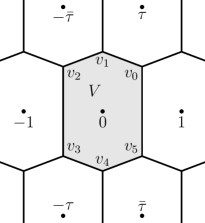
  Figure 3.1. Voronoi cell $V$ of $0$ corresponding to the set $\mathbbm{Z}[\tau]$ with $\tau=\frac{1}{2}+\frac{i}{2}\sqrt{7}$ (i.e., $p=1$, $q=2$).

• The vertices of $V$ are

  $$v_{0} =\frac{p}{2}+\frac{i}{2\mathop{{\operatorname{Im}}\thinspace\negthinspace}\mathchoice{\negthinspace}{\negthinspace}{}{}\left({\tau}\right)}\left(\mathop{{\operatorname{Im}}\thinspace\negthinspace}\mathchoice{\negthinspace}{\negthinspace}{}{}\left({\tau}\right)^{2}-\frac{1}{4}\right)=\frac{p}{2}+\frac{i}{\sqrt{4q-1}}\left(q-\frac{1}{2}\right)\!,$$

  $$v_{1} =\frac{i}{2\mathop{{\operatorname{Im}}\thinspace\negthinspace}\mathchoice{\negthinspace}{\negthinspace}{}{}\left({\tau}\right)}\left(\mathop{{\operatorname{Im}}\thinspace\negthinspace}\mathchoice{\negthinspace}{\negthinspace}{}{}\left({\tau}\right)^{2}+\frac{1}{4}\right)=\frac{i}{\sqrt{4q-1}}q,$$

  $$v_{2} =-\frac{p}{2}+\frac{i}{2\mathop{{\operatorname{Im}}\thinspace\negthinspace}\mathchoice{\negthinspace}{\negthinspace}{}{}\left({\tau}\right)}\left(\mathop{{\operatorname{Im}}\thinspace\negthinspace}\mathchoice{\negthinspace}{\negthinspace}{}{}\left({\tau}\right)^{2}-\frac{1}{4}\right)=-\frac{p}{2}+\frac{i}{\sqrt{4q-1}}\left(q-\frac{1}{2}\right)\!,$$

  and $v_{3}=-v_{0}$, $v_{4}=-v_{1}$ and $v_{5}=-v_{2}$, see Heuberger and Krenn [10].

• Let $w$ be an integer with $w\geq 2$. We call $w$ the window size of our expansions, see also Definition 2.1.

• Let

  $$d=\frac{v_{1}-v_{0}}{\left\lvert{v_{1}-v_{0}}\right\rvert}$$

  be the direction from $v_{0}$ to $v_{1}$, and note that we have

  $$d=pi\frac{\tau}{\sqrt{q}}.$$

  Set $d_{w}=d(\tau/\sqrt{q})^{w}$. See also Figure 3.2.

• Let

  $$s=\sqrt{\frac{q-1/4}{q+2}}$$

  be the height of the rectangle defined below. See also Figure 3.2.

• Define the open rectangle $R_{w}$ with vertices

  • $\tau^{w}v_{0}+d_{w}\sqrt{q}$,

  • $\tau^{w}v_{1}-d_{w}\sqrt{q}$,

  • $\tau^{w}v_{1}-d_{w}\sqrt{q}-pid_{w}s$, and

  • $\tau^{w}v_{0}+d_{w}\sqrt{q}-pid_{w}s$.

  An example of this rectangle is shown in Figure 3.2.

  

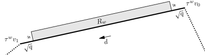
  Figure 3.2. Rectangle $R_{5}$ for $q=5$ and $p=1$.

  Note that one side length of the rectangle $R_{w}$ is

  $$\left\lvert{\tau^{w}v_{1}-\tau^{w}v_{0}}\right\rvert-2\sqrt{q}=\sqrt{q}^{w}\frac{1}{2}\sqrt{1+\frac{1}{4q-1}}-2\sqrt{q}=\sqrt{\frac{q^{w+1}}{4q-1}}-2\sqrt{q}$$ (3.1)

  and the other is $s$.

We finish this section with a couple of remarks.

Remark 3.1.

The location of the rectangle $R_{w}$ (in relation to the scaled Voronoi cell $\tau^{w}V$) is in such a way that $\tau^{-1}R_{w}$ has empty intersection with $\tau^{w}V$. When constructing the actual counterexample in Part III, this will guarantee us that an element of $R_{w}$ does not become a digit (during division by $\tau$).

Remark 3.2.

Note that the rectangle $R_{w}$ is well defined (has positive area) if and only if $w>\log(16q-4)/\log q$, which follows from positivity of (3.1). Therefore, for $q=2$ we have $w\geq 5$, for $q=3$ we have $w\geq 4$, for $4\leq q\leq 15$ we have $w\geq 3$ and for $q\geq 16$ we have $w\geq 2$.

4. Lattices

As mentioned above, our digit expansions live in the lattice

$$\mathbbm{Z}[\tau]=\left\{{*}\right\}{a+b\tau}{\text{$a\in\mathbbm{Z}$, $b\in\mathbbm{Z}$}}=\langle 1,\tau\rangle.$$

It will become handy to define a few other (related) lattices. Our first one is

$$\Lambda_{\tau}=\langle\tau,q-p\tau\rangle=\langle\tau,\tau^{2}\rangle,$$

where we interpret the complex plane embedded into $\mathbbm{R}^{2}$ in the usual way. This lattice is used during the construction of our counterexamples, since we need points divisible by $\tau$ there. Further, we also work with the smaller lattice

$$\Lambda_{\tau^{2}}=\langle\tau^{2},\tau^{3}\rangle=\langle q\tau,\tau^{2}\rangle\subseteq\Lambda_{\tau},$$

since in view of Proposition 5.1 we want to avoid this lattice.

Moreover, let us note that the middle point of the lower long side of the rectangle $R_{w}$ is

$$\frac{v_{0}+v_{1}}{2}\tau^{w}=\frac{\tau^{w+1}}{2}.$$

In general this is not a point of the lattice $\Lambda_{\tau}$ but of the lattice

$$\Lambda_{\tau/2}=\frac{1}{2}\Lambda_{\tau}=\langle\frac{\tau}{2},\frac{\tau^{2}}{2}\rangle\supseteq\Lambda_{\tau}.$$

This is the reason why we will work mainly in the larger lattice $\Lambda_{\tau/2}$.

We need some basic properties of the lattices above. Let us start with $\Lambda_{\tau}$ and some divisibility conditions for its elements.

Lemma 4.1.

The elements of $\mathbbm{Z}[\tau]$ divisible by $\tau$ once (i.e., divisible by $\tau$ but not by $\tau^{2}$) are exactly the elements

$$a\tau+b(q-p\tau)$$

with $a\in\mathbbm{Z}$ but $q\mathbin{\nmid}a$ and with $b\in\mathbbm{Z}$.

Moreover, if $z\in\mathbbm{Z}[\tau]$ is a lattice point divisible by $\tau$, then $z-1$, $z+1$, $z+\tau-p$ and $z-\tau+p$ are not divisible by $\tau$.

The structures described above can be found in Figure 4.1.

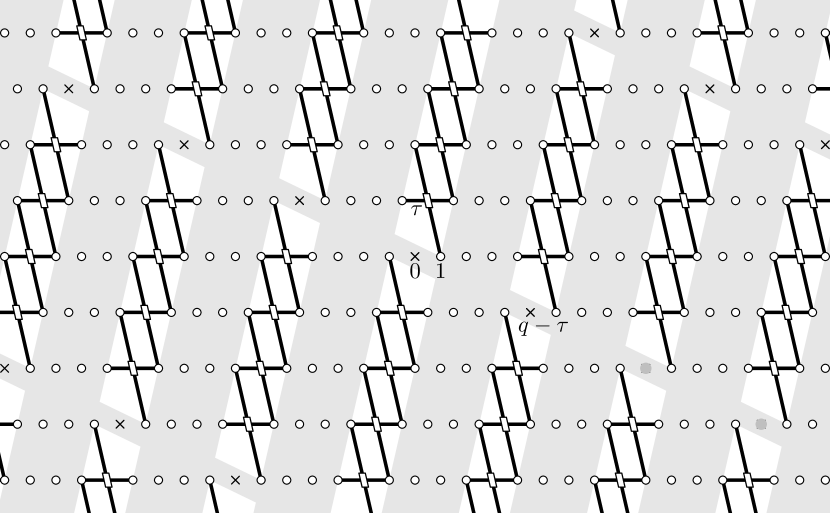
Figure 4.1. Lattice $\mathbbm{Z}[\tau]$. Points marked with a circle are not divisible by $\tau$, points marked with a rectangle are divisible exactly once by $\tau$, points marked with a cross are divisible by $\tau^{2}$. There are lines from each rectangle (divisible exactly once by $\tau$) to its neighboring circles (not divisible by $\tau$)

.

Proof of Lemma 4.1.

An element $c+d\tau\in\mathbbm{Z}[\tau]$ is divisible by $\tau$ if and only if $q\mathbin{\mid}c$. Therefore, if $z\in\mathbbm{Z}[\tau]$ is divisible by $\tau$, then $z-1$, $z+1$, $z+\tau-p$ and $z-\tau+p$ are not divisible by $\tau$, which proves the second part of the lemma. As $\tau\mathbin{\nmid}a-b\tau$ if and only if $q\mathbin{\nmid}a$, multiplying by $\tau$ yields the first part of the lemma. ∎

For analyzing the lattice $\Lambda_{\tau/2}$ and the scaled Voronoi cell $\tau^{w}V$, it is important to know some arithmetic properties of $\tau$. We show the following lemma to get some insights.

Lemma 4.2.

The algebraic integer $\tau$ satisfies the following properties.

1. Every prime $\ell\in\mathbbm{Z}$ with $\ell\mathbin{\mid}q$ splits in $\mathbbm{Z}[\tau]$.

2. If $a$ and $b$ are integers with $a+b\tau=\tau^{w}$ or $a+b\tau=\bar{\tau}^{w}$, then $\gcd(a,b)=1$.

Note that $\mathbbm{Z}[\tau]$ is the maximal order of $\mathbbm{Q}(\tau)$.

Proof of Lemma 4.2.

The first statement is a direct consequence from algebraic number theory, in particular the splitting of a prime $\ell$ in $\mathbbm{Z}[\tau]$ is described by the factorization of the minimal polynomial of $\tau$ mod $\ell$ (for example, see Theorem 2 in Chapter 11 of Ribenboim [23]). Indeed we have

$$X^{2}-pX+q\equiv X^{2}\pm X\equiv X(X\pm 1)\mod\ell,$$

hence all primes $\ell\mathbin{\mid}q$ split completely in $\mathbbm{Z}[\tau]$.

The second statement is trivial for $w\in\left\{{0,1}\right\}$ (note that we use $w\geq 2$ throughout this paper anyway). Suppose $a$ and $b$ have a common prime factor $\ell$, then $\ell$ also has to divide $\mathop{{\mathcal{N}}\thinspace\negthinspace}\mathchoice{\negthinspace}{\negthinspace}{}{}\left({\bar{\tau}}\right)^{w}=\mathop{{\mathcal{N}}\thinspace\negthinspace}\mathchoice{\negthinspace}{\negthinspace}{}{}\left({\tau}\right)^{w}=q^{w}$ (where $\mathop{{\mathcal{N}}\thinspace\negthinspace}\mathchoice{\negthinspace}{\negthinspace}{}{}\left({\tau}\right)$ denotes the norm of $\tau$). Thus $\ell\mathbin{\mid}q$. By using part (1) of this lemma we have $(\ell)=\mathfrak{p}\bar{\mathfrak{p}}$ as ideals over $\mathbbm{Z}[\tau]$.

Let us assume for a moment that both $\mathfrak{p}$ and $\bar{\mathfrak{p}}$ divide $(\tau)$, then also both $\mathfrak{p}$ and $\bar{\mathfrak{p}}$ divide $(\bar{\tau})$, i.e., $\tau,\bar{\tau}\in\mathfrak{p}\bar{\mathfrak{p}}=(\ell)$. But this yields $\ell\mathbin{\mid}\tau+\bar{\tau}=p$, a contradiction. Therefore let us assume now that $\mathfrak{p}\mathbin{\mid}(\tau)$ and $\bar{\mathfrak{p}}\mathbin{\nmid}(\tau)$. Since by assumption $a$ and $b$ have the common factor $\ell$, they also have the common factor $\bar{\mathfrak{p}}$ form the ideal point of view, hence $\bar{\mathfrak{p}}\mathbin{\mid}(\tau)^{w}$ if $a+b\tau=\tau^{w}$, a contradiction to the previous discussion. Similarly, we get the contradiction $\mathfrak{p}\mathbin{\mid}(\bar{\tau})^{w}$ for the case $a+b\tau=\bar{\tau}^{w}$. ∎

It is also important to know that no lattice points are on the “lower” edge of $R_{w}$. This result is also used to show the uniqueness of the digit set, see Proposition 12.2.

Lemma 4.3.

The following two statements hold.

1. The only lattice point in $\Lambda_{\tau/2}$ lying on the line segment joining the points $v_{0}\tau^{w}$ and $v_{1}\tau^{w}$ is $\frac{1}{2}\tau^{w+1}$.

2. The boundary of $\tau^{w}V$ has empty intersection with the lattice $\mathbbm{Z}[\tau]$.

Proof.

We start by showing that there are no lattice points of $\Lambda_{1/2}=\langle\frac{1}{2},\frac{\tau}{2}\rangle$ except $\frac{1}{2}\tau^{w}$ on the line going through $v_{5}\tau^{w}$ and $v_{0}\tau^{w}$. Every point on this line can be written as $\frac{1}{2}\tau^{w}+ti\tau^{w}$ with some real parameter $t$. Let us assume we have a point $\lambda=\frac{1}{2}\tau^{w}+a\frac{1}{2}+b\frac{\tau}{2}$ with $a$, $b\in\mathbbm{Z}$ on this line. Furthermore, we may assume that $\gcd(a,b)=1$ (as a minimality condition). We deduce $2ti\tau^{w}=a+b\tau$.

If $i\in\mathbbm{Q}(\tau)$, then $4q-1$ is a perfect square which is absurd since $4q-1\equiv-1\mod 4$. Let us write $\tau^{w}=a_{w}+b_{w}\tau$, then Lemma 4.2 yields $\gcd(a_{w},b_{w})=1$. Thus, and since $i\not\in\mathbbm{Q}(\tau)$, the only possible values for $t$ are $\pm\frac{1}{2}$. Indeed $2ti\tau^{w}$ is an algebraic integer and therefore we have $2t\in\mathbbm{Z}[\tau]\cap\mathbbm{R}=\mathbbm{Z}$ with $t\neq 0$ and $|t|<1$. Now, we obtain a contradiction, since $\lambda=\frac{1}{2}(1\pm i)\tau^{w}$ is not in $\Lambda_{1/2}$.

The results are now obtained as follows. Multiplying everything by $\tau$ yields the first statement of the lemma. Starting with $\frac{1}{2}\tau^{w+1}+ti\tau^{w+1}$ yields that there are no points from $\Lambda_{1/2}$ except $\frac{1}{2}\tau^{w+1}$ on the line joining $v_{0}\tau^{w}$ and $v_{1}\tau^{w}$. Note that this differs from the first statement of the lemma by the different lattice. The result for the third line (from $v_{1}\tau^{w}$ to $v_{2}\tau^{w}$) follows by taking conjugation and Lemma 4.2 with $\bar{\tau}^{w}=a_{w}+b_{w}\tau$. The remaining three sides of $\tau^{w}V$ follow by mirroring. ∎

We are also interested in the shortest vector in the lattice $\Lambda_{\tau/2}$.

Lemma 4.4.

The shortest nonzero vectors in the lattice $\Lambda_{\tau/2}$ are $\pm\tau/2$.

Proof.

First, let us note that $\big{\lvert}{\frac{\tau}{2}}\big{\rvert}=\frac{\sqrt{q}}{2}$. To find the shortest nonzero vector $a\frac{\tau}{2}+b\frac{\tau^{2}}{2}\in\Lambda_{\tau/2}$ we have to find all integers $a$ and $b$ such that $\big{\lvert}{a\frac{\tau}{2}+b\frac{\tau^{2}}{2}}\big{\rvert}\leq\frac{\sqrt{q}}{2}$. In particular we have to solve the inequality

$$\left\lvert{a+b\tau}\right\rvert^{2}=\Bigl{(}a+b\frac{p}{2}\Bigr{)}^{2}+b^{2}\Bigl{(}q-\frac{1}{4}\Bigr{)}\leq 1.$$

Obviously, if $b\neq 0$, then this inequality cannot be satisfied. Thus we may assume that $b=0$. We obtain $a^{2}\leq 1$, and the result follows. ∎

Part II The Diophantine Part

5. Overview

In this part of the article we show that the following proposition holds.

Proposition 5.1.

We use the set-up described in Section 3 with the following restrictions. Suppose we are in one of the cases

• $q\in\left\{{2,4}\right\}$ and $w\geq 7$,

• $q\in\left\{{3}\right\}$ and $w\geq 5$ or

• $5\leq q\leq 500$ and $w\geq 4$.

Then there exists a lattice point

$$a\tau+b(q-p\tau)$$

with $a\in\mathbbm{Z}$, $q\mathbin{\nmid}a$ and with $b\in\mathbbm{Z}$ in the (open) rectangle $R_{w}$.

Since the proof of this proposition is long and technical, we start with an overview. In a nutshell, for fixed $q$, we can reduce the problem to checking only finitely many configurations $w$. Therefore the testing is possible algorithmically.

Let us look at an outline of the ideas used during the proof a bit. The resulting algorithm takes as input parameters $q$ and $p$ and returns a list of values for $w$ which have to be investigated by other methods (i.e., yet no lattice point was found for these $w$). The details can be found in the last section of this part, Section 10. In order to make this algorithm work, we have to check Proposition 5.1 for all but finitely many cases.

One major step to tackle this lemma is to reduce the lattice point problem into a Diophantine approximation problem. We show this in Section 9. The existence result of the lattice points there is based on the theory of the geometry of numbers. More precisely, this gives us two lattice points (see Lemma 9.3) out of which we can construct a lattice point avoiding a smaller lattice (as it is required by Proposition 5.1), see Lemma 9.5. But, to make this work, we have to use linear independence of the two points, which is the challenging part during the proof.

We can reformulate this linear independence problem geometrically, which leaves us to show that there are no lattice points inside a certain smaller rectangle. To solve it, we bring this Diophantine approximation problem into a favorable form, which leaves us to show that the inequalities

$$\left\lvert{\log\left(\frac{a+b\tau}{\left\lvert{a+b\tau}\right\rvert}\right)-w\log\left(\frac{\tau}{\left\lvert{\tau}\right\rvert}\right)+k\frac{i\pi}{2}}\right\rvert<\chi q^{2-w/2}$$ (5.1a)

with $$\chi=9$$ and

$$\left\lvert{a+b\tau}\right\rvert<\psi q^{2}$$ (5.1b)

with $\psi=4$ have no integer solutions.

With the previous inequality linear forms in logarithms come into play. The theory to solve this problem, unfortunately, provides only solutions for huge $w$ (and fixed $q$), see Section 7. The words “unfortunately” and “huge” here mean that it is not possible to test the remaining finitely many configurations in reasonable time. In order to reduce the bounds from which on (5.1) does not have any integer solutions (and thus reducing the calculation time), we use a method due to Baker and Davenport [5] in Section 8.

We are left with a bunch of small cases. Some remarks on how to check the lemma for these values directly can be found in Section 6.

Note that the steps above were presented in reverse ordering (from the perspective, that we only use results, which were proven earlier in the article), since this is more the way one has to think when solving such a problem.

6. Testing Directly

In this section, we collect some remarks on how to directly test whether Proposition 5.1 holds for fixed parameters. So let us fix $q$, $p$ and $w$. We use the following criterion to find a lattice point $\lambda\in\Lambda_{\tau}\setminus\Lambda_{\tau^{2}}$ inside the rectangle $R_{w}$.

We first establish necessary and sufficient conditions for a complex number $z=x+iy$ to be contained in $R_{w}$.

Proposition 6.1.

Set

$$B_{1} =\frac{q^{w+1}}{4},$$

$$B_{2} =\frac{q^{w+1}}{4}+\frac{q^{(w+1)/2}}{2}\sqrt{\frac{q-1/4}{q+2}}$$

and

$$B_{3} =\frac{q^{w+1}}{2(4q-1)}-\frac{q^{w/2+1}}{\sqrt{4q-1}},$$

and let us write $\frac{1}{2}\tau^{w+1}=u_{w}+v_{w}\tau$. Then $\lambda=a\tau+b\tau^{2}\in R_{w}$ if and only if

$$B_{1}<a\left(\frac{u_{w}p}{2}+v_{w}q\right)+b\left(\frac{u_{w}}{2}-u_{w}q+\frac{v_{w}pq}{2}\right)<B_{2}$$ (6.1a)

and

$$\left\lvert{au_{w}+b(u_{w}p+v_{w}q)}\right\rvert<B_{3}.$$ (6.1b)

We can solve this system of inequalities and obtain finitely many pairs of integers $(a,b)$. If we find a pair with $q\mathbin{\nmid}a$, then Proposition 5.1 is true for this instance. Thus, Proposition 6.1 leads to a “searching algorithm” to solve Proposition 5.1 for a particular parameter set.

Proof.

Let $\frac{1}{2}\tau^{w+1}=x_{w}+iy_{w}$. By elementary geometry we know that a point $(x,y)$ that lies between the upper and lower length sides of $R_{w}$ satisfies

$$\left(\frac{\left\lvert{\tau}\right\rvert^{w+1}}{2}\right)^{2}<xx_{w}+yy_{w}<\frac{\left\lvert{\tau}\right\rvert^{w+1}}{2}\left(\frac{\left\lvert{\tau}\right\rvert^{w+1}}{2}+s\right)\!.$$

Since

$$x_{w}+iy_{w}=u_{w}+\frac{v_{w}p}{2}+iv_{w}\sqrt{q-1/4}$$

and since we want to have constraints for integers $a$ and $b$ in $(x,y)$ with

$$x+iy=\lambda=a\tau+b\tau^{2}=\frac{ap}{2}+\frac{b}{2}-bq+i(a+bp)\sqrt{q-1/4},$$

we obtain

$$xx_{w}+yy_{w}=a\left(\frac{u_{w}p}{2}+\frac{v_{w}}{4}\right)+b\left(\frac{1}{2}-q\right)\left(u_{w}+\frac{v_{w}p}{2}\right)+(a+bp)v_{w}\left(q-\frac{1}{4}\right)\!,$$

from which (6.1a) follows.

The inequality for $(x,y)$ being in between the sides of $R_{w}$ parallel to $\tau^{w}$ is given by

$$\left\lvert{xy_{w}-yx_{w}}\right\rvert<\frac{\left\lvert{\tau}\right\rvert^{w+1}}{2}\left(\frac{\left\lvert{v_{0}-v_{1}}\right\rvert\left\lvert{\tau}\right\rvert^{w}}{2}-\sqrt{q}\right)=B_{3}\sqrt{q-1/4}$$

and, likewise as above, we have

$$xy_{w}-yx_{w}=\left(a\frac{v_{w}p}{2}+bv_{w}\left(\frac{1}{2}-q\right)-(a+bp)\left(u_{w}+\frac{v_{w}p}{2}\right)\right)\sqrt{q-1/4}.$$

The inequality (6.1b) follows.

Therefore the lattice point $\lambda\in\Lambda_{\tau}\cap R_{w}$ satisfies both inequalities stated in the lemma and, the other way round, all such points are inside $R_{w}$. ∎

7. Huge Bounds for $w$

This section deals with showing that the Inequalities (5.1) have no integer solutions. We do this by providing a method to find for a fixed $q$ all $w$ such that (5.1) is satisfied. More precisely, we will give a (rather huge) bound on $w$ such that solutions (if any) are only possible for smaller values.

However, for a single fixed $q$ we still have (too) many possiblities to test all $w$, see Lemma 7.2 below and the text afterwards. Therefore we will reduce the upper bound of $w$ by using a variant of the Baker–Davenport method [5] in Section 8.

We can restrict ourselves to the following setting. We may assume $b>0$ since otherwise $-a$, $-b$ and $w$ would satisfy (5.1). Moreover, we may assume that $\gcd(a,b)=1$. If $a$ and $b$ would have a common divisor $d$ then with $a$, $b$ and $w$ also $a/d$, $b/d$ and $w$ would satisfy (5.1).

As a first step we want to find a bound for $w$ for a fixed integer $q\geq 2$.

Proposition 7.1.

For every $q$ there exists an explicitly computable bound $w_{q}$ such that the Inequalities (5.1) do not have any integer solutions with $w\geq w_{q}$.

The following lemma states the precise conditions when solutions of (5.1) are possible. Proposition 7.1 is a direct consequence of this result.

Lemma 7.2.

Solutions to (5.1) exist only if

$$7.72\cdot 10^{13}\log q\log(\sqrt{\psi}q)\log\left(4.87w\frac{\max\{3\pi,2\log q\}}{\log(\sqrt{\psi}q)}\right)\\ >-\log\chi+\frac{w-4}{2}\log q$$ (7.1)

with $\chi=9$ and $\psi=4$ holds.

In particular, for

$$w \geq 8.68\cdot 10^{15}\log q\log\log q q\geq 13$$ if

and

$$w \geq 1.973\cdot 10^{16} q\in\left\{{2,3,\dots,12}\right\}$$ if

the Inequalities (5.1) do not have any integer solutions.

It is easy to see that for fixed $q$ the Inequality (7.1) cannot hold if $w$ is large. For instance $q=2$ yields $w\leq w_{2}=8.596\cdot 10^{15}$ or for $q=42$ we obtain $w\leq w_{42}=2.747\cdot 10^{16}$. This is one of the key results used in the proof of our main result, Theorem 2.3.

In the following, we denote by $\mathop{{h}\thinspace\negthinspace}\mathchoice{\negthinspace}{\negthinspace}{}{}\left({\alpha}\right)$ the absolute logarithmic height, which is defined as follows. Let $\alpha$ be an algebraic number of degree $d$ and with minimal polynomial

$$a_{0}\prod_{i=1}^{d}\left(X-\alpha_{i}\right),$$

then

$$\mathop{{h}\thinspace\negthinspace}\mathchoice{\negthinspace}{\negthinspace}{}{}\left({\alpha}\right)=\frac{1}{d}\Big{(}\log\left\lvert{a_{0}}\right\rvert+\sum_{i=1}^{d}\max\{0,\log\left\lvert{\alpha_{i}}\right\rvert\}\Big{)}.$$

For the proof of Lemma 7.2 and in view of (5.1) we apply the following result due to Matveev [16].

Theorem 7.3 (Theorem 2.2 with $r=1$ in [16]).

Denote by $\alpha_{1}$, …, $\alpha_{n}$ algebraic numbers, not $0$ nor $1$, by $\log\alpha_{1}$, …, $\log\alpha_{n}$ determinations of their logarithms, by $D$ the degree over $\mathbbm{Q}$ of the number field $K=\mathbbm{Q}(\alpha_{1},\ldots,\alpha_{n})$, and by $b_{1}$, …, $b_{n}$ rational integers. Furthermore let $\kappa=1$ if $K$ is real and $\kappa=2$ otherwise. For all integers $j$ with $1\leq j\leq n$ choose

$$A_{j}\geq\max\left\{{D\mathop{{h}\thinspace\negthinspace}\mathchoice{\negthinspace}{\negthinspace}{}{}\left({\alpha_{j}}\right),\left\lvert{\log\alpha_{j}}\right\rvert,0.16}\right\},$$

and set

$$B=\max\left\{{1}\right\}\cup\left\{{*}\right\}{\left\lvert{b_{j}}\right\rvert A_{j}/A_{n}}{1\leq j\leq n}.$$

Assume that

$$b_{1}\log\alpha_{1}+\cdots+b_{n}\log\alpha_{n}\not=0.$$

Then

$$\log\left\lvert{b_{1}\log\alpha_{1}+\cdots+b_{n}\log\alpha_{n}}\right\rvert\geq-C(n,\kappa)\max\left\{{1,n/6}\right\}C_{0}W_{0}D^{2}\Omega$$

with

$$\Omega=A_{1}\cdots A_{n},$$

$$C(n,\kappa)=\frac{16}{n!\,\kappa}e^{n}(2n+1+2\kappa)(n+2)(4(n+1))^{n+1}\left(\frac{1}{2}en\right)^{\kappa},$$

$$C_{0}=\log\left(e^{4.4n+7}n^{5.5}D^{2}\log(eD)\right),\quad W_{0}=\log(1.5eBD\log(eD)).$$

Proof of Lemma 7.2.

We observe that in Matveev’s theorem we have $n=3$, $D=4$ and $\kappa=2$ since we use

$$\alpha_{3}=\frac{a+b\tau}{\left\lvert{a+b\tau}\right\rvert},\qquad\alpha_{2}=\frac{\tau}{\left\lvert{\tau}\right\rvert}\qquad\text{and}\qquad\alpha_{3}=i.$$

Moreover, we set $b_{3}=1$, $b_{2}=-w$ and $b_{1}=k$.

Next, let us compute the heights of $\frac{a+b\tau}{\left\lvert{a+b\tau}\right\rvert}$ and $\frac{\tau}{\left\lvert{\tau}\right\rvert}$. Let us note that for an imaginary quadratic integer $\alpha$ the algebraic number $\alpha/|\alpha|$ is a zero of

$$\left\lvert{\alpha}\right\rvert^{4}(X-\alpha/\left\lvert{\alpha}\right\rvert)(X-\bar{\alpha}/\left\lvert{\alpha}\right\rvert)(X+\alpha/\left\lvert{\alpha}\right\rvert)(X+\bar{\alpha}/\left\lvert{\alpha}\right\rvert)$$

and therefore

$$\mathop{{h}\thinspace\negthinspace}\mathchoice{\negthinspace}{\negthinspace}{}{}\left({\frac{\alpha}{\left\lvert{\alpha}\right\rvert}}\right)=\frac{1}{4}\left(\log\left\lvert{a_{0}}\right\rvert+4\log\left\lvert{\alpha/\left\lvert{\alpha}\right\rvert}\right\rvert\right)\leq\log\left\lvert{\alpha}\right\rvert$$ (7.2)

since $\left\lvert{a_{0}}\right\rvert\leq\left\lvert{\alpha}\right\rvert^{4}$. We choose

$$A_{3} =8\log(\sqrt{\psi}q)=4\log(\psi q^{2})\geq 4\log\left\lvert{a+b\tau}\right\rvert,$$

$$A_{2} =2\log q=4\log\left\lvert{\tau}\right\rvert,$$

$$A_{1} =2\pi=4\left\lvert{\log i}\right\rvert.$$

Next we find an upper bound for $k$. Let us note that $\left\lvert{\log\frac{a+b\tau}{\left\lvert{a+b\tau}\right\rvert}}\right\rvert<2\pi$ and from the consideration above we have

$$\left\lvert{\log\frac{\tau}{\left\lvert{\tau}\right\rvert}}\right\rvert\leq\pi-\arctan(\sqrt{4q-1})\leq\frac{2\pi}{3}.$$

Therefore, a very crude estimate of inequality (5.1a) yields

$$\left\lvert{2\pi+w\frac{2\pi}{3}-k\frac{\pi}{2}}\right\rvert<\frac{\pi}{2},$$

and, thus, $k\leq\frac{3w}{2}$. We choose

$$B=w\frac{\max\{3\pi,2\log q\}}{A_{3}}.$$

Before we may apply Theorem 7.3 we have to check that our linear form in logarithms (i.e., the left hand side of (5.1a)) is nonzero. Let us assume for the moment the contrary. But assuming that the linear form in logarithms is zero expressed in geometric terms is that $\frac{1}{2}\tau^{w+1}+\frac{1}{2}(a\tau+b\tau^{2})$ lies on the line segment joining the points $v_{0}\tau^{w}$ and $v_{1}\tau^{w}$, thus equals $\frac{1}{2}\tau^{w+1}$, which contradicts Lemma 4.3. In view of inequality (5.1a) and Theorem 7.3 we obtain (7.1).

We are left to compute the explicit bounds for $w$. Let us assume for the moment that $\max\{3\pi,2\log q\}=2\log q$, i.e., that $q\geq 112>e^{3\pi/2}$. Let us note that under this assumption we have $\log(\sqrt{\psi}q)<1.15\log q$. By a crude estimate we deduce that Inequality (7.1) is not satisfied if

$$1.954\cdot 10^{14}\log q\log w<w$$ (7.3)

holds, unless $w<10^{10}$. Due to a result of Pethő and de Weger [20], namely their Lemma 2.2, an inequality of the form $A\log x\geq x$ with $A>e^{2}$ implies the inequality $x<2A\log A$. Therefore we find an explicit bound for $w$, namely

$$w\geq 8.68\cdot 10^{15}\log q\log\log q>3.908\cdot 10^{14}\log q\log\bigl{(}1.954\cdot 10^{14}\log q\bigr{)},$$

which implies (7.3) and consequently the non-existence of solutions.

By solving inequality (7.1) for each integer $2\leq q<112$ one can easily show that the explicit bounds stated in the Lemma also hold for $q<112$. ∎

Proof of Proposition 7.1.

The result follows out of Lemma 7.2 since for fixed $q$ Inequality (7.1) does not hold if $w$ is sufficiently large. ∎

8. Reducing the Bounds for $w$

The bounds from the previous section (Proposition 7.1) are too huge in order to test all remaining configurations in reasonable time. Now our aim is to reduce these bounds which is done below and works very well: For instance, the bound $w_{2}=8.596\cdot 10^{15}$ is reduced to $\widetilde{w}_{2}=140$. We modify a method due to Baker and Davenport [5] to succeed, see Lemma 8.1 for details.

The remaining section deals with special cases and the occurrence of some linear dependence in the linear form in logarithms. Lemma 8.2 allows us to test for this linear dependence and in Lemma 8.3 we describe how to deal with this situation. At the end, we deal with two special cases (Lemma 8.4).

Let us denote the distance to the nearest integer by $\left\lVert{\,\cdot\,}\right\rVert$.

Lemma 8.1.

Suppose we have a bound $w_{q}$ for $w$ (i.e., Inequalities (5.1) do not have any integer solutions for $w\geq w_{q}$). Fix $a$ and $b$. Let $P/Q$ be a convergent to

$$\epsilon=\frac{2}{i\pi}\log\frac{\tau}{\left\lvert{\tau}\right\rvert}$$

with the properties that $\left\lVert{Q\epsilon}\right\rVert=\kappa/w_{q}$ for some $\kappa<1/4$, but $\left\lVert{Q\delta}\right\rVert>2\kappa$, where

$$\delta=\frac{2}{i\pi}\log\frac{a+b\tau}{\left\lvert{a+b\tau}\right\rvert}.$$

Then the Inequalities (5.1) do not have any integer solutions with our fixed $a$ and $b$, and with

$$w\geq\widetilde{w}_{a,b}=\frac{2}{\log q}\log\left(\frac{2\chi Q}{\kappa\pi}\right)+4,$$

where $\chi=9$.

Note that $\kappa<1/4$ is formally not needed as an assumption in the lemma, but $\left\lVert{Q\delta}\right\rVert>2\kappa$ implies this condition.

Proof of Lemma 8.1.

Assume that $w_{q}>w\geq\widetilde{w}_{a,b}$ is satisfied and that we have a solution of (5.1). We multiply Inequality (5.1a) by $2Q/\pi$ and use the notations of the lemma to obtain

$$\left\lvert{Q\delta-wQ\epsilon+k}\right\rvert<\frac{2\chi Q}{\pi}q^{2-w/2}\leq\kappa.$$

But on the other hand, we have

$$\left\lvert{Q\delta-wQ\epsilon+k}\right\rvert\geq\left\lVert{Q\delta}\right\rVert-w\left\lVert{Q\epsilon}\right\rVert>2\kappa-w\frac{\kappa}{w_{q}}>\kappa.$$

Combining these two inequalities yields a contradiction. ∎

We want to emphasize that Lemma 8.1 yields bounds only in case of $\epsilon$ and $\delta$ are linearly independent over $\mathbbm{Q}$. If this is not the case, then the considerations in the remaining section can be used. In particular, this is the case if $b=0$ or $2a+bp=0$ holds.

The following lemma allows us to test the linear dependence of $\log\bigl{(}\frac{\tau}{\left\lvert{\tau}\right\rvert}\bigr{)}$ and $\log\bigl{(}\frac{a+b\tau}{\left\lvert{a+b\tau}\right\rvert}\bigr{)}$ over $\mathbbm{Q}$.

Lemma 8.2.

Suppose we have integers $a$ and $b$ such that $m=|a+b\tau|^{2}<\psi^{2}q^{4}$ with $\psi=4$. Let us write $q=d_{1}d_{2}^{2}$ and $m=m_{1}m_{2}^{2}$, such that $d_{2}$ and $m_{2}$ are maximal with respect to $\gcd(d_{1},d_{2})=\gcd(m_{1},m_{2})=1$. Set $m^{\prime}=m_{1}/\gcd(m_{1},d_{1})$. With $\nu_{\ell}$ being the $\ell$-adic valuation, set $\alpha_{\ell}=\nu_{\ell}(q)$ for all primes $\ell\mathbin{\mid}q$. For odd primes $\ell\mathbin{\mid}q$ let $\alpha^{\prime}_{\ell}=\alpha_{\ell}$ if $\ell\mathbin{\mid}d_{1}m^{\prime}$ and put $\alpha^{\prime}_{\ell}=\alpha_{\ell}/2$ otherwise. If $2\mathbin{\mid}q$ we put

$$\alpha^{\prime}_{2}=\begin{cases}\alpha_{2}/2&\quad{\@displayfalse\text{if $d_{1}\equiv m^{\prime}\equiv 1\!\!\mod 4$,}}\\ \alpha_{2}&\quad{\@displayfalse\text{if $2\mathbin{\mid}d_{1}m^{\prime}$ and if $d_{1}\equiv 1\!\!\mod 4$ or $m^{\prime}\equiv 1\!\!\mod 4$,}}\\ \alpha_{2}&\quad{\@displayfalse\text{if $2\mathbin{\nmid}d_{1}m^{\prime}$ and if $d_{1}\equiv 3\!\!\mod 4$ or $m^{\prime}\equiv 3\!\!\mod 4$,}}\\ 2\alpha_{2}&\quad{\@displayfalse\text{if $2\mathbin{\mid}d_{1}m^{\prime}$ and if $d_{1}\equiv 3\!\!\mod 4$ or $m^{\prime}\equiv 3\!\!\mod 4$.}}\end{cases}$$

Let $N$ be the greatest common divisor of all $\alpha^{\prime}_{\ell}$ with primes $\ell\mathbin{\mid}q$.

Then $\log\bigl{(}\frac{\tau}{\left\lvert{\tau}\right\rvert}\bigr{)}$ and $\log\bigl{(}\frac{a+b\tau}{\left\lvert{a+b\tau}\right\rvert}\bigr{)}$ are linearly dependent over $\mathbbm{Q}$ if and only if

$$\left(\frac{\tau}{\left\lvert{\tau}\right\rvert}\right)^{\eta}=\left(\frac{a+b\tau}{\left\lvert{a+b\tau}\right\rvert}\right)^{\vartheta}$$ (8.1)

for some positive integer $\vartheta\mathbin{\mid}24N$ and some integer $\eta$ with $\left\lvert{\eta}\right\rvert<\vartheta\bigl{(}4+\frac{2\log\psi}{\log q}\bigr{)}$.

Proof.

It is immediate that $\log\bigl{(}\frac{\tau}{\left\lvert{\tau}\right\rvert}\bigr{)}$ and $\log\bigl{(}\frac{a+b\tau}{\left\lvert{a+b\tau}\right\rvert}\bigr{)}$ are linearly dependent over $\mathbbm{Q}$ if and only if (8.1) holds. First, let us consider (8.1) as an equation in the ideal group of the field $K=\mathbbm{Q}(\tau,\sqrt{d_{1}},\sqrt{m^{\prime}})$.

We aim to compute the prime ideal factorization of $(\ell)$ for every prime $\ell\mathbin{\mid}q$. We already know by Lemma 4.2 that every such ideal $(\ell)$ splits in $\mathbbm{Q}(\tau)$ and is therefore unramified. Furthermore, by definition $d_{1}$ and $m^{\prime}$ are coprime; therefore, $(\ell)$ with an odd prime $\ell\mathbin{\mid}q$ is at most in one of the fields $\mathbbm{Q}(\sqrt{d_{1}})$ and $\mathbbm{Q}(\sqrt{m^{\prime}})$ ramified. Hence, $(\ell)$ is ramified in $K$ if and only if $\ell\mathbin{\mid}d_{1}m^{\prime}$. Moreover, if the ideal $(\ell)$ is ramified, then the ramification index is exactly two. Altogether we get the following by using the fact that $K$ is an Abelian extension of $\mathbbm{Q}$.

• If $\ell\mathbin{\nmid}d_{1}m^{\prime}$, then $(\ell)=\mathcal{J}_{\ell}\bar{\mathcal{J}}_{\ell}$, where $\mathcal{J}_{\ell}\mathbin{\mid}(\tau)$ is the product of distinct prime ideals.

• If $\ell\mathbin{\mid}d_{1}m^{\prime}$, then $(\ell)=\mathcal{J}_{\ell}^{2}\bar{\mathcal{J}}_{\ell}^{2}$, where $\mathcal{J}_{\ell}\mathbin{\mid}(\tau)$ is the product of distinct prime ideals.

Let us turn to the case $\ell=2$. Recall that the ideal $(2)$ ramifies in the quadratic field $\mathbbm{Q}(\sqrt{d})$ if and only if $d\equiv 2\!\!\mod 4$ or $d\equiv 3\!\!\mod 4$. We have to distinguish between several cases.

• First, let us assume that the ideal $(2)$ neither ramifies in $\mathbbm{Q}(\sqrt{d_{1}})$ nor in $\mathbbm{Q}(\sqrt{m^{\prime}})$ (and consequently not in $\mathbbm{Q}(\sqrt{d_{1}m^{\prime}})$ either), i.e., $d_{1}\equiv m^{\prime}\equiv 1\mod 4$. Then $(2)$ is also unramified in $K$ and we have $(2)=\mathcal{J}_{2}\bar{\mathcal{J}}_{2}$, where $\mathcal{J}_{2}$ is the product of distinct prime ideals.

• There is no situation, when the ideal $(2)$ ramifies in exactly one of the fields $\mathbbm{Q}(\sqrt{d_{1}})$, $\mathbbm{Q}(\sqrt{m^{\prime}})$ and $\mathbbm{Q}(\sqrt{d_{1}m^{\prime}})$.

• Next, suppose the ideal $(2)$ is ramified in exactly two of the fields $\mathbbm{Q}(\sqrt{d_{1}})$, $\mathbbm{Q}(\sqrt{m^{\prime}})$ and $\mathbbm{Q}(\sqrt{d_{1}m^{\prime}})$., i.e., one of the two cases

  • $2\mathbin{\mid}d_{1}m^{\prime}$ together with $d_{1}\equiv 1\mod 4$ or $m^{\prime}\equiv 1\mod 4$, or

  • $2\mathbin{\nmid}d_{1}m^{\prime}$ together with $d_{1}\equiv 3\mod 4$ or $m^{\prime}\equiv 3\mod 4$

  occurs. Then $(2)=\mathcal{J}_{2}^{2}\bar{\mathcal{J}}_{2}^{2}$, where $\mathcal{J}_{2}$ is the product of distinct prime ideals.

• If the ideal $(2)$ is ramified in all of the fields $\mathbbm{Q}(\sqrt{d_{1}})$, $\mathbbm{Q}(\sqrt{m^{\prime}})$ and $\mathbbm{Q}(\sqrt{d_{1}m^{\prime}})$, i.e., $2\mathbin{\mid}d_{1}m^{\prime}$ together with $d_{1}\equiv 3\mod 4$ or $m^{\prime}\equiv 3\mod 4$, then $(2)=\mathcal{J}_{2}^{4}\bar{\mathcal{J}}_{2}^{4}$, where $\mathcal{J}_{2}$ is some prime ideal.

Therefore, by considering the definition of $\alpha^{\prime}_{\ell}$, we obtain

$$(\tau)=\prod_{\begin{subarray}{c}\ell\mathbin{\mid}q\\ \text{$\ell$ prime}\end{subarray}}\mathcal{J}_{\ell}^{2\alpha^{\prime}_{\ell}}.$$

Note that $\alpha^{\prime}_{\ell}=\alpha_{\ell}/2$ only happens if $\alpha_{\ell}$ is even. Furthermore we obtain

$$\left(\frac{\tau}{\left\lvert{\tau}\right\rvert}\right)=\prod_{\begin{subarray}{c}\ell\mathbin{\mid}q\\ \text{$\ell$ prime}\end{subarray}}\left(\frac{\mathcal{J}_{\ell}}{\bar{\mathcal{J}}_{\ell}}\right)^{\alpha^{\prime}_{\ell}}\!.$$

Therefore $\bigl{(}\frac{\tau}{\left\lvert{\tau}\right\rvert}\bigr{)}$ is an $N$th power if and only if $N$ divides the greatest common divisor of all $\alpha^{\prime}_{\ell}$ with primes $\ell\mathbin{\mid}q$.

Let us turn now from the ideal group point of view to the element point of view of Equation (8.1). So far we have proved that $\log\bigl{(}\frac{\tau}{\left\lvert{\tau}\right\rvert}\bigr{)}$ and $\log\bigl{(}\frac{a+b\tau}{\left\lvert{a+b\tau}\right\rvert}\bigr{)}$ are linearly independent over $\mathbbm{Q}$ if and only if there exist integers $\vartheta$ and $\eta$ such that

$$\left(\frac{\tau}{\left\lvert{\tau}\right\rvert}\right)^{\eta}\left(\frac{a+b\tau}{\left\lvert{a+b\tau}\right\rvert}\right)^{-\vartheta}=1$$

and $\vartheta\mathbin{\mid}N$. Set $n=\gcd(\eta,\vartheta)$. By taking $n$th roots we obtain

$$\left(\frac{\tau}{\left\lvert{\tau}\right\rvert}\right)^{\eta/n}\left(\frac{a+b\tau}{\left\lvert{a+b\tau}\right\rvert}\right)^{-\vartheta/n}=\zeta_{n},$$ (8.2)

where $\zeta_{n}$ is an $n$th root of unity. The group $\operatorname{Gal}(\mathbbm{Q}(\zeta_{n})/\mathbbm{Q})$ is a subgroup of $\operatorname{Gal}(K/\mathbbm{Q})$, and $\operatorname{Gal}(K/\mathbbm{Q})$ is isomorphic to a subgroup of $(\mathbbm{Z}/2\mathbbm{Z})^{3}$. Since $24$ is maximal with $\varphi(24)=8$ (where $\varphi$ is Euler’s phi function), we deduce that $n\mathbin{\mid}24$. If we take Equation (8.2) to the $24$th power, we obtain the first statement of the lemma.

Because of (7.2) we have heights

$$\mathop{{h}\thinspace\negthinspace}\mathchoice{\negthinspace}{\negthinspace}{}{}\left({\frac{\tau}{\left\lvert{\tau}\right\rvert}}\right)=\frac{1}{2}\log q$$

and

$$\mathop{{h}\thinspace\negthinspace}\mathchoice{\negthinspace}{\negthinspace}{}{}\left({\frac{a+b\tau}{\left\lvert{a+b\tau}\right\rvert}}\right)\leq\log\left\lvert{a+b\tau}\right\rvert=\log\sqrt{m}<\log\psi+2\log q.$$

Comparing these heights on the left and right side of (8.1) we obtain

$$\frac{\eta}{2}\log q=\eta\mathop{{h}\thinspace\negthinspace}\mathchoice{\negthinspace}{\negthinspace}{}{}\left({\frac{\tau}{\left\lvert{\tau}\right\rvert}}\right)=\vartheta\mathop{{h}\thinspace\negthinspace}\mathchoice{\negthinspace}{\negthinspace}{}{}\left({\frac{a+b\tau}{\left\lvert{a+b\tau}\right\rvert}}\right)<\vartheta(\log\psi+2\log q).$$

∎

Lemma 8.3.

Suppose we have a bound $w_{q}$ for $w$ (i.e., Inequalities (5.1) do not have any integer solutions for $w\geq w_{q}$), and suppose that we have for fixed $a$ and $b$ a linear dependence of the form

$$\eta\log\left(\frac{\tau}{\left\lvert{\tau}\right\rvert}\right)=\vartheta\mathop{{\log}\thinspace\negthinspace}\mathchoice{\negthinspace}{\negthinspace}{}{}\left({\frac{a+b\tau}{\left\lvert{a+b\tau}\right\rvert}}\right)\!,$$

such that $\vartheta>0$.

1. Let $P/Q$ be an expanded fraction of a convergent (i.e., $P/Q=P^{\prime}/Q^{\prime}$ for a convergent $P^{\prime}/Q^{\prime}$) to $\epsilon=\frac{2}{\pi}\log\bigl{(}\frac{\tau}{\left\lvert{\tau}\right\rvert}\bigr{)}$ with the following properties. Suppose $W_{Q}=(Q+\eta)/\vartheta$ is largest possible with $W_{Q}<w_{q}$ (i.e., $Q<w_{q}\vartheta-\eta$) and $W_{Q}\in\mathbbm{Z}$ such that

   $$Q\left\lvert{\epsilon-P/Q}\right\rvert<\frac{2\chi\vartheta}{\pi}q^{2-W_{Q}/2}$$ (8.3)

   with $\chi=9$ holds. If no such fraction $P/Q$ exists, then set $W_{Q}=-\infty$.

2. Let $W$ be the smallest positive integer such that the inequality

   $$\frac{2\chi\vartheta}{\pi}q^{2-W/2}\leq\frac{1}{2(W\vartheta-\eta)}$$ (8.4)

   with $\chi=9$ holds.

Then the Inequalities (5.1) do not have any integer solutions with our fixed $a$ and $b$, and with

$$w\geq\widetilde{w}_{a,b}=\max\{W_{Q}+1,W\}.$$

Proof.

The assumption on the linear dependence yields an inequality of the form

$$\left\lvert{(w\vartheta-\eta)\log\left(\frac{\tau}{\left\lvert{\tau}\right\rvert}\right)-\vartheta k\frac{i\pi}{2}}\right\rvert<\chi\vartheta q^{2-w/2}$$ (8.5)

or with the notation of Lemma 8.1,

$$\left\lvert{\epsilon-\frac{\vartheta k}{w\vartheta-\eta}}\right\rvert<\frac{2\chi\vartheta}{(w\vartheta-\eta)\pi}q^{2-w/2}.$$ (8.6)

Note that due to a well-known Theorem of Legendre we have the following: If

$$\frac{2\chi\vartheta}{(w\vartheta-\eta)\pi}q^{2-w/2}\leq\frac{1}{2(w\vartheta-\eta)^{2}},$$

which is true for large enough $w$, then $(\vartheta k)/(w\vartheta-\eta)=P^{\prime}/Q^{\prime}$, where $P^{\prime}/Q^{\prime}$ is a convergent to $\epsilon$. Since $P^{\prime}$ and $Q^{\prime}$ are coprime, we have $Q^{\prime}\mathbin{\mid}w\vartheta-\eta$, so $w\vartheta-\eta=Q$ for some multiple $Q$ of $Q^{\prime}$. ∎

Lemma 8.4.

Suppose we have a bound $w_{q}$ for $w$ (i.e., Inequalities (5.1) do not have any integer solutions for $w\geq w_{q}$) and suppose that $a=1$ and either $b=0$ or $b=-2p$. Let $P/Q$ be an expanded fraction of a convergent (i.e., $P/Q=P^{\prime}/Q^{\prime}$ for a convergent $P^{\prime}/Q^{\prime}$) to $\epsilon=\frac{2}{\pi}\log\bigl{(}\frac{\tau}{\left\lvert{\tau}\right\rvert}\bigr{)}$ with the following properties. Suppose $W_{Q}=Q$ is largest possible with $W_{Q}<w_{q}$ (i.e., $Q<w_{q}$) such that

$$Q\left\lvert{\epsilon-P/Q}\right\rvert<\frac{2\chi}{\pi}q^{2-W_{Q}/2}$$

with $\chi=9$ holds. If no such convergent exists, then set $W_{Q}=-\infty$.

Then the Inequalities (5.1) do not have any integer solutions with our fixed $a$ and $b$ as above, and with

$$w\geq\widetilde{w}_{a,b}=\max\{W_{Q}+1,25\}.$$

Note that the bound $25$ is sharp for $q=2$, but for $q>2$ a better bound could be chosen.

Proof of Lemma 8.4.

In both cases $\log\bigl{(}\frac{a+b\tau}{\left\lvert{a+b\tau}\right\rvert}\bigr{)}$ is an integral multiple of $\frac{i\pi}{2}$. Therefore, we consider the inequality

$$\left\lvert{w\log\left(\frac{\tau}{\left\lvert{\tau}\right\rvert}\right)-k\frac{i\pi}{2}}\right\rvert<\chi q^{2-w/2}$$ (8.7)

which is similar to (8.5). In the same way as before (proof of Lemma 8.3) and with the notation of Lemma 8.1 we obtain

$$\left\lvert{\epsilon-\frac{k}{w}}\right\rvert<\frac{2\chi}{w\pi}q^{2-w/2}$$

and that $\frac{k}{w}$ equals a convergent $P^{\prime}/Q^{\prime}$ to $\epsilon$ if

$$\frac{2\chi}{w\pi}q^{(-w+4)/2}\leq\frac{1}{2w^{2}}$$ (8.8)

which is true for large $w$, in particular for all $w\geq 25$. Therefore a solution $w\geq 25$ to Inequalities (5.1) corresponds to a fraction $P/Q=P^{\prime}/Q^{\prime}$ such that $Q=w$. ∎

In order to get a reduced bound $\widetilde{w}_{q}$, we look at all possible combinations of $a$ and $b$ and calculate a bound $\widetilde{w}_{a,b}$ by the lemmata and considerations above. The bound $\widetilde{w}_{q}$ is the maximum of all these bounds.

9. Geometry of Numbers

The theory of the geometry of numbers is used to show the existence of a lattice point in the rectangle $R_{w}$ with the desired properties (i.e., out of the lattice $\Lambda_{\tau}$ but not in $\Lambda_{\tau^{2}}$). We use two other rectangles inside $R_{w}$, one which is wide but low (called $\widetilde{R}_{\mathrm{WL}}$) and one which is narrow but high (called $\widetilde{R}_{\mathrm{NH}}$). Minkowski’s lattice point theorem (Theorem 9.2) gives us the existence of a lattice point inside each of these two rectangles (see Lemma 9.3), and we are able to construct our desired lattice point out of it (Lemma 9.5), provided that the two found points are linearly independent. This is guaranteed if the intersection of the two mentioned rectangles with $\Lambda_{\tau/2}$ only contains $\tau^{w+1}/2$, which follows from the Inequalities (5.1) by Lemma 9.1. So much for a short overview on this section; let us begin.

We use the lattices $\Lambda_{\tau}$ and $\Lambda_{\tau/2}$, which were defined in Section 4. Throughout this section, we further use the rectangle $\widetilde{R}_{\mathrm{NH}}$ with vertices

$$\frac{\tau^{w+1}}{2}\pm i\frac{\tau^{w+1}}{\left\lvert{\tau}\right\rvert^{w+1}}q^{2}\sqrt{q+2}$$

and

$$\frac{\tau^{w+1}}{2}+\frac{\tau^{w+1}}{\left\lvert{\tau}\right\rvert^{w+1}}\frac{s}{4q}\pm i\frac{\tau^{w+1}}{\left\lvert{\tau}\right\rvert^{w+1}}q^{2}\sqrt{q+2}$$

with $s=\sqrt{\frac{q-1/4}{q+2}}$, and the rectangle $\widetilde{R}_{\mathrm{WL}}$ with vertices

$$\frac{\tau^{w+1}}{2}\pm i\frac{\tau^{w+1}}{\left\lvert{\tau}\right\rvert^{w+1}}\frac{1}{16q}\frac{q^{(w+1)/2}}{\sqrt{q-\tfrac{1}{4}}}$$

and

$$\frac{\tau^{w+1}}{2}+\frac{\tau^{w+1}}{\left\lvert{\tau}\right\rvert^{w+1}}\cdot 4q^{(3-w)/2}\bigl{(}q-\tfrac{1}{4}\bigr{)}\pm i\frac{\tau^{w+1}}{\left\lvert{\tau}\right\rvert^{w+1}}\frac{1}{16q}\frac{q^{(w+1)/2}}{\sqrt{q-\tfrac{1}{4}}}.$$

Note that these two rectangles are both contained in (the closure) of $R_{w}$. See also Figure 9.1.

In the Lemmata 9.1, 9.4 and 9.5 we need that (at least) one of the conditions

(9.1)

on $q$ and $w$ holds. These bounds are sharp in Lemma 9.4.

Lemma 9.1.

Suppose $q$ and $w$ satisfy Conditions (9.1). If Inequalities (5.1) do not have any integer solutions (for given $q$ and $w$), then the only lattice point of $\Lambda_{\tau/2}$ in $\widetilde{R}_{\mathrm{NH}}\cap\widetilde{R}_{\mathrm{WL}}$ is $\tau^{w+1}/2$.

Since by construction $\widetilde{R}_{\mathrm{NH}}\cap\widetilde{R}_{\mathrm{WL}}$ is a rectangle with side lengths

$$2q^{2}\sqrt{q+2}\qquad\text{and}\qquad 4q^{(3-w)/2}\bigl{(}q-\tfrac{1}{4}\bigr{)},$$ (9.2)

therefore has an area which decreases with $w$, it seems very reasonable to assume that the only lattice point contained in $\widetilde{R}_{\mathrm{NH}}\cap\widetilde{R}_{\mathrm{WL}}$ is $\frac{1}{2}\tau^{w+1}$. In order to prove this result, we reformulate this geometric problem into a problem from Diophantine analysis (finding solutions for Inequalities (5.1)).

Proof of Lemma 9.1.

First let us note that the shortest vector of $\Lambda_{\tau/2}$ is $\frac{\tau}{2}$ which has length $\sqrt{q}/2$ (see Lemma 4.4). Therefore the angle between the lower long side of $R_{w}$ and $\lambda\in\widetilde{R}_{\mathrm{NH}}\cap\widetilde{R}_{\mathrm{WL}}$ with $\lambda\neq\frac{\tau^{w+1}}{2}$ is at most

$$\arcsin\frac{4q^{(3-w)/2}\bigl{(}q-\tfrac{1}{4}\bigr{)}}{\tfrac{1}{2}\sqrt{q}}=\mathop{{\arcsin}\thinspace\negthinspace}\mathchoice{\negthinspace}{\negthinspace}{}{}\big{(}{8q^{2-w/2}\bigl{(}1-\tfrac{1}{4q}\bigr{)}}\big{)}$$ (9.3)

in absolute values. Due to the conditions (9.1), the argument of the arcsine is less than $0.11$ and we have $\arcsin(x)<9x/8$; we obtain an upper bound for that angle. On the other hand the angle between the vector $\tau^{w}$ and $a+b\tau$ is

$$\big{\lvert}{\arg{a+b\tau}-\arg{\tau^{w}}}\big{\rvert}=\left\lvert{\log\!\left(\frac{a+b\tau}{|a+b\tau|}\right)-\log\!\left(\frac{\tau^{w}}{|\tau^{w}|}\right)}\right\rvert\\ =\left\lvert{\log\!\left(\frac{a+b\tau}{|a+b\tau|}\right)-w\log\!\left(\frac{\tau}{|\tau|}\right)+k\frac{i\pi}{2}}\right\rvert$$

for some integer $k$. This together with Inequality (9.3) yields Inequality (5.1a).

Now let us write $\lambda=\frac{1}{2}\tau^{w+1}+\frac{1}{2}(a\tau+b\tau^{2})$. Further, by 9.2 we know that

$$\left\lvert{\tfrac{\tau}{2}(a+b\tau)}\right\rvert^{2}\leq q^{5}\bigl{(}1+\tfrac{2}{q}\bigr{)}+16q^{5-w}\bigl{(}1-\tfrac{1}{4q}\bigr{)}^{2}<4q^{5}$$

provided that $w\geq 4$. Thus

$$\left\lvert{a+b\tau}\right\rvert<\psi q^{2}$$

with $\psi=4$ and $a$ and $b$ are bounded in terms of $q$. All together we obtain Inequalities (5.1). ∎

In order to find at least one point inside each of the rectangles $\widetilde{R}_{\mathrm{NH}}$ and $\widetilde{R}_{\mathrm{WL}}$ we use Minkowski’s lattice point theorem (for example, see Theorem II in Chapter III of Cassels [7]).

Theorem 9.2 (Minkowski’s lattice point theorem).

Let $S\subset\mathbbm{R}^{n}$ be a compact point set of volume $V$ which is symmetric about the origin and convex. Let $\Lambda$ be any $n$-dimensional lattice with lattice constant $\mathop{{d}\thinspace\negthinspace}\mathchoice{\negthinspace}{\negthinspace}{}{}\left({\Lambda}\right)$. If $V\geq 2^{n}\mathop{{d}\thinspace\negthinspace}\mathchoice{\negthinspace}{\negthinspace}{}{}\left({\Lambda}\right)$ then there exists a pair of points $\pm\lambda\in\Lambda\cap S$, with $\lambda\neq 0$.

Figure 9.1. The rectangles $\widetilde{R}_{\mathrm{NH}}$ and $\widetilde{R}_{\mathrm{WL}}$, and points $\lambda_{\mathrm{NH}}$ and $\lambda_{\mathrm{WL}}$.

Lemma 9.3.

For $j\in\left\{{\mathrm{NH},\mathrm{WL}}\right\}$ there exists a lattice point $\lambda_{j}\in\Lambda_{\tau/2}$ in the rectangle $\widetilde{R}_{j}$.

The situation of this lemma is show in Figure 9.1.

Proof.

First, note that the lattice $\Lambda_{\tau/2}$ has lattice constant

$$\mathop{{d}\thinspace\negthinspace}\mathchoice{\negthinspace}{\negthinspace}{}{}\left({\Lambda_{\tau/2}}\right)=\tfrac{1}{4}\mathop{{d}\thinspace\negthinspace}\mathchoice{\negthinspace}{\negthinspace}{}{}\left({\Lambda_{\tau}}\right)=\tfrac{1}{4}q\sqrt{q-\tfrac{1}{4}}.$$

Let us mirror the rectangle $\widetilde{R}_{\mathrm{NH}}$ on the line joining the points $v_{0}\tau^{w}$ and $v_{1}\tau^{w}$, and consider the rectangle $\widetilde{R}_{\mathrm{NH}}$ joint with the mirrored rectangle. We obtain a compact, symmetric around $\frac{1}{2}\tau^{w+1}$, convex set (a rectangle) of volume

$$2\frac{s}{4q}\cdot 2q^{2}\sqrt{q+2}=q\sqrt{q-\tfrac{1}{4}}=4\mathop{{d}\thinspace\negthinspace}\mathchoice{\negthinspace}{\negthinspace}{}{}\left({\Lambda_{\tau/2}}\right).$$

Now Minkowski’s lattice point theorem yields a $\lambda_{\mathrm{NH}}\in\widetilde{R}_{\mathrm{NH}}\cap\Lambda_{\tau/2}$.

Let us construct $\lambda_{\mathrm{WL}}$ similarly: Again we mirror the rectangle $\widetilde{R}_{\mathrm{WL}}$ on the line joining the points $v_{0}\tau^{w}$ and $v_{1}\tau^{w}$ and consider the rectangle $\widetilde{R}_{\mathrm{WL}}$ joint with the mirrored rectangle. We obtain a compact, symmetric around $\frac{1}{2}\tau^{w+1}$, convex set again of volume

$$2\cdot 4q^{(3-w)/2}\bigl{(}q-\tfrac{1}{4}\bigr{)}\cdot 2\frac{1}{8q}\frac{q^{(w+1)/2}}{\sqrt{q-\tfrac{1}{4}}}=q\sqrt{q-\tfrac{1}{4}}=4\mathop{{d}\thinspace\negthinspace}\mathchoice{\negthinspace}{\negthinspace}{}{}\left({\Lambda_{\tau/2}}\right).$$

Minkowski’s lattice point theorem yields a $\lambda_{\mathrm{WL}}\in\widetilde{R}_{\mathrm{WL}}\cap\Lambda_{\tau/2}$. ∎

From now on we assume that we have $\lambda_{\mathrm{NH}}$ and $\lambda_{\mathrm{WL}}$ as in Lemma 9.3. The following result is needed in the proof of Lemma 9.5.

Lemma 9.4.

Suppose $q$ and $w$ satisfy Conditions (9.1). Then all lattice points of the form

$$\frac{\tau^{w+1}}{2}+a\left(\lambda_{\mathrm{NH}}-\frac{\tau^{w+1}}{2}\right)+b\left(\lambda_{\mathrm{WL}}-\frac{\tau^{w+1}}{2}\right)$$

with non-negative integers $a$ and $b$ at most $2q$ are contained in the rectangle $R_{w}$.

Proof.

All given points are contained in $R_{w}$ if the two inequalities

$$2q\cdot q^{2}\sqrt{q+2}+2q\cdot\frac{1}{16q}\frac{q^{(w+1)/2}}{\sqrt{q-\tfrac{1}{4}}}<\frac{1}{2}\sqrt{\frac{q^{w+1}}{4q-1}}-\sqrt{q}$$

and

$$2q\cdot\frac{s}{4q}+2q\cdot 4q^{(3-w)/2}\bigl{(}q-\tfrac{1}{4}\bigr{)}<s$$

with $s=\sqrt{\frac{q-1/4}{q+2}}$ are satisfied. This is the case for the given conditions. ∎

With the construction above (and the assumptions of Lemma 9.4) we are in a position to prove the following Lemma.

Lemma 9.5.

Suppose $q$ and $w$ satisfy Conditions (9.1). If

$$\widetilde{R}_{\mathrm{NH}}\cap\widetilde{R}_{\mathrm{WL}}\cap\Lambda_{\tau/2}=\left\{{\tfrac{1}{2}\tau^{w+1}}\right\},$$

then there exists a $\lambda\in R_{w}$ with $\lambda\in\Lambda_{\tau}\setminus\Lambda_{\tau^{2}}$.

Proof.

First we show that the lattice points $\mu_{\mathrm{NH}}=\lambda_{\mathrm{NH}}-\frac{1}{2}\tau^{w+1}$ and $\mu_{\mathrm{WL}}=\lambda_{\mathrm{WL}}-\frac{1}{2}\tau^{w+1}$ are linearly independent. Let us shift the origin to $\frac{1}{2}\tau^{w+1}$ and let us rotate the coordinate system such that the long “lower side” of the rectangle $R_{w}$, which contains the origin, is parallel to the real axis. In this new coordinate system, we write $\hat{\lambda}_{\mathrm{NH}}$ and $\hat{\lambda}_{\mathrm{WL}}$ for $\lambda_{\mathrm{NH}}$ and $\lambda_{\mathrm{WL}}$ respectively. We have $\big{\lvert}{\mathop{{\operatorname{Re}}\thinspace\negthinspace}\mathchoice{\negthinspace}{\negthinspace}{}{}\big{(}{\hat{\lambda}_{\mathrm{NH}}}\big{)}}\big{\rvert}<\big{\lvert}{\mathop{{\operatorname{Re}}\thinspace\negthinspace}\mathchoice{\negthinspace}{\negthinspace}{}{}\big{(}{\hat{\lambda}_{\mathrm{WL}}}\big{)}}\big{\rvert}$ and $0<\mathop{{\operatorname{Im}}\thinspace\negthinspace}\mathchoice{\negthinspace}{\negthinspace}{}{}\big{(}{\hat{\lambda}_{\mathrm{WL}}}\big{)}<\mathop{{\operatorname{Im}}\thinspace\negthinspace}\mathchoice{\negthinspace}{\negthinspace}{}{}\big{(}{\hat{\lambda}_{\mathrm{NH}}}\big{)}$, i.e., $\lambda_{\mathrm{NH}}$ and $\lambda_{\mathrm{WL}}$ are not colinear and therefore $\mu_{\mathrm{NH}}$ and $\mu_{\mathrm{WL}}$ are linearly independent.

Since we know now that $\mu_{\mathrm{NH}}$ and $\mu_{\mathrm{WL}}$ are linearly independent, there exists a basis $\nu_{1}$, $\nu_{2}$ of $\Lambda_{\tau/2}$ such that

$$\mu_{\mathrm{NH}}=\alpha_{11}\nu_{1}\qquad\text{and}\qquad\mu_{\mathrm{WL}}=\alpha_{21}\nu_{1}+\alpha_{22}\nu_{2}$$

with $0<\alpha_{11}$ and $0\leq\alpha_{21}<\alpha_{22}$. In our case this means there exists a basis $\nu_{1},\nu_{2}$ for $\Lambda_{\tau/2}$ such that $\nu_{1}$ and $\nu_{2}$ are contained in the parallelogram with vertices $0$, $\mu_{\mathrm{NH}}$, $\mu_{\mathrm{WL}}$ and $\mu_{\mathrm{NH}}+\mu_{\mathrm{WL}}$. Moreover, by the assumptions of the lemma and Lemma 9.4 all lattice points of the form $\lambda=\frac{\tau^{w+1}}{2}+a\nu_{1}+b\nu_{2}\in\Lambda_{\tau/2}$ with $0\leq a\leq 2q$ and $0\leq b\leq 2q$ are contained in the rectangle $R_{w}$.

Now let us write

$$\nu_{1}=\beta_{11}\tau+\beta_{12}\tau^{2}\qquad\text{and}\qquad\nu_{2}=\beta_{21}\tau+\beta_{22}\tau^{2}.$$

Since $\nu_{1}$ and $\nu_{2}$ as well as $\tau$ and $\tau^{2}$ are bases to the same lattice $\Lambda_{\tau}$ we conclude that $\begin{pmatrix}\beta_{11}&\beta_{12}\\ \beta_{21}&\beta_{22}\end{pmatrix}\in\mathrm{SL}_{2}(\mathbbm{Z})$. Our aim is to show that there exist non-negative integers $a$ and $b$ at most $2q$ such that $\lambda\in\Lambda_{\tau}$ but $\lambda\not\in\Lambda_{\tau^{2}}$. Setting

$$\tfrac{1}{2}\tau^{w+1}=u_{w}\frac{\tau}{2}+v_{w}\frac{\tau^{2}}{2},$$

it suffices to prove that

$$\left(u_{w}+a\beta_{11}+b\beta_{12}\right)\frac{\tau}{2}+\left(v_{w}+a\beta_{21}+b\beta_{22}\right)\frac{\tau^{2}}{2}=\gamma_{1}\frac{\tau}{2}+\gamma_{2}\frac{\tau^{2}}{2}$$

for some $\gamma_{1}\equiv 2\mod 2q$ and $\gamma_{2}\equiv 0\mod 2q$ has a solution. But a solution can be found from a solution to the linear system

$$u_{w}+a\beta_{11}+b\beta_{12} =2$$

$$v_{w}+a\beta_{21}+b\beta_{22} =0$$

modulo $2q$. Such a solution certainly exists since $\begin{pmatrix}\beta_{11}&\beta_{12}\\ \beta_{21}&\beta_{22}\end{pmatrix}\in\mathrm{SL}_{2}(\mathbbm{Z})$. ∎

With the previous results, we are ready to prove the following proposition.

Proposition 9.6.

For every $q$ there exists an explicitly computable bound $w_{q}$ such that for each $w\geq w_{q}$ there exists a lattice point

$$a\tau+b(q-p\tau)$$

with $a\in\mathbbm{Z}$, $q\mathbin{\nmid}a$ and with $b\in\mathbbm{Z}$ in the rectangle $R_{w}$.

Proof.

Proposition 7.1 states a similar result for the non-existence of solutions of Inequalities (5.1). By Lemma 9.1 this translates to having the single intersection point $\frac{1}{2}\tau^{w+1}$ in the rectangles $\widetilde{R}_{\mathrm{NH}}$ and $\widetilde{R}_{\mathrm{WL}}$. This condition is then used in Lemma 9.5 to find a lattice point inside $R_{w}$ as desired. ∎

10. An Algorithm to Test for fixed $q$

In order to prove Proposition 5.1 for given $q$ and $p$, but all $w$—this means showing the existence of a lattice point in each rectangle $R_{w}$ with the stated properties—we apply the following algorithm

Algorithm 10.1.

We fix $q$ and fix a choice of $p\in\left\{{-1,1}\right\}$ as input. This algorithm returns a list of values for $w$ for which no lattice point in $R_{w}$ exists. We proceed as follows.

1. Compute an upper bound $w_{q}$ for possible solutions (with $w<w_{q}$) using Matveev’s Theorem 7.3 and in particular Inequality (7.1).

2. Reduce the bound $w_{q}$ by the Baker–Davenport method (Section 8).

   1. Compute sufficiently many (consecutive) convergents $P/Q$ to $\epsilon=\frac{2}{i\pi}\log\frac{\tau}{\left\lvert{\tau}\right\rvert}$ and save them in a list $\mathcal{L}$. Precalculate and save $\kappa$ with $\left\lVert{Q\epsilon}\right\rVert=\kappa/w_{q}$ as well.

   2. Use Lemma 8.4 to deal with the case $2a+bp=0$ (i.e., $a=1$, $b=-2p$) and compute the new bounds $\widetilde{w}_{a,b}$.

   3. For all integers $a$, $b$ with $\left\lvert{a+b\tau}\right\rvert<\psi q^{2}$, $\psi=4$ and with $b>0$, coprime $a$, $b$ and excluding the situations from step 2b do the following:

      1. Find $\eta$ and $\vartheta$ such that

         $$\left(\frac{\tau}{\left\lvert{\tau}\right\rvert}\right)^{\eta}=\left(\frac{a+b\tau}{\left\lvert{a+b\tau}\right\rvert}\right)^{\vartheta}$$

         using Lemma 8.2.

      2. If such $\eta$ and $\vartheta$ do not exist in step 2(c)i, find the convergents $P/Q$ in $\mathcal{L}$ with smallest $Q$ that satisfies $\kappa<\frac{1}{4}$ and $\left\lVert{Q\delta}\right\rVert>2\kappa$ with $\delta=\frac{2}{i\pi}\log\frac{a+b\tau}{\left\lvert{a+b\tau}\right\rvert}$. Compute the new bound $\widetilde{w}_{a,b}$ due to Lemma 8.1.

      3. If such $\eta$ and $\vartheta$ in step 2(c)i exist, find an expanded fraction $P/Q$ of the convergents in $\mathcal{L}$ with largest $Q$ that satisfies $W_{Q}=(Q+\eta)/\vartheta\leq w_{q}$ and (8.4). Compute the new bound $\widetilde{w}_{a,b}$ due to Lemma 8.3.

   4. Calculate $\widetilde{w}_{q}$ as the maximum of all $\widetilde{w}_{a,b}$.

3. For all $4\leq w<\widetilde{w}_{q}$ (with exceptions obtained by taking into account the assumptions of Proposition 5.1), we verify Proposition 5.1 directly as described in Section 6.

Note that Algorithm 10.1 as it is written is not guaranteed to terminate. The reason is that it might be impossible to find a convergent $P/Q$ with the desired properties in step 2(c)ii. Stopping this search at some point and not using the reduced bound of step 2 will make the algorithm terminate for sure. However, a huge amount of $w$ have to be checked in step 3 then.

Proposition 10.2.

Let $q\geq 2$. If Algorithm 10.1 terminates, then it is correct, i.e., it returns a list of values for $w$ for which no lattice point in $R_{w}$ with the properties stated in Proposition 5.1 exists.

Proof.

Section 9 reduces the problem of finding lattice points in $R_{w}$ to showing that Inequalities (5.1) do not have any integer solutions. Step 1 provides a bound for $w$; it can be computed effectively according to Proposition 7.1. Step 2 reduces this bound. We get a bound for each possible combination of $a$ and $b$ (all the different cases are analyzed in Section 8); correctly determining whether we have a linear dependence is done via Lemma 8.2.

Taking the maximum of all these bounds yields $\widetilde{w}_{q}$, a new bound. In step 3 all remaining $w$ are checked by a direct search according to Proposition 6.1. Since this proposition finds a lattice point if and only if one exists, we are able to classify all the $w$ and return a list of the exceptional values. ∎

Proof of Proposition 5.1.

We apply Algorithm 10.1. ∎

Part III The Part with the Digits

11. Overview

In this part of the article, we construct the actual counterexamples to the minimality of the width-$w$ non-adjacent forms (see Section 2 for the relevant definitions). This means we have to find an expansion of a lattice point with a lower number of nonzero digits than the width-$w$ non-adjacent form ($w$-NAF) of this point.

We reuse the ideas of Heuberger and Krenn [12] for our construction. This work also tells us that (if it exists) a counterexample using a (multi-)expansion of weight two can be found. Therefore, we will try to find

$$A\tau^{w-1}+B=C\tau^{w}+D=E\tau^{2w}+F\tau^{w}+G,$$ (11.1)

where the most left and the most right parts of the equation are valid digit expansions, i.e., $A$, $B$, $E$, $F$ and $G$ are digits. Moreover, we assume that $D$ is a digit (equal to $G$), but, in order to get a counterexample to minimality, $C$ is not allowed to be a digit. However, the point $C$ is important during the construction of this counterexample: we will have $C=E\tau^{w}+F$ and $D=G$, and, more important, there will be a change $\Delta$ with $\tau C=A+\Delta$ and $D=B-\Delta\tau^{w-1}$.

Some explicit constructions are given in Section 13 and Proposition 17.1, but most of the time we will consider a more general situation. There, the existence of a construction like above relies on Proposition 5.1, which was proven in the previous part. This lemma gives us the point $C$. The change $\Delta$ is discussed in Section 14, and Section 15 deals with the digits $B$, $D$ and $G$. Everything is glued together in Sections 16 and 17.

We begin with a section which deals with the digit set we use. Note that this digit set is strongly related to the Voronoi cell defined in Section 3.

12. Digit Sets

In this section, we make a formal definition of the used digit set. This is equivalent to the definition stated in Section 2 but uses the Voronoi cell to model the minimal norm property. Afterwards we show that this choice of digits is unique.

Definition 12.1 (Minimal Norm Digit Set).

Let $w$ be an integer with $w\geq 2$ and $\mathcal{D}\subseteq\mathbbm{Z}[\tau]$ consist of $0$ and exactly one representative of each residue class of $\mathbbm{Z}[\tau]$ modulo $\tau^{w}$ that is not divisible by $\tau$. If all such representatives $\eta\in\mathcal{D}$ satisfy $\eta\in\tau^{w}V$, then $\mathcal{D}$ is called the minimal norm digit set modulo $\tau^{w}$.

The minimal norm digit set above is uniquely determined, see below.

Proposition 12.2.

Let $\mathcal{D}$ be a minimal norm digit set modulo $\tau^{w}$. Then $\mathcal{D}$ is uniquely determined. In particular, there exists a unique element of minimal norm in each residue class modulo $\tau^{w}$ which is not divisible by $\tau$.

This proposition was proved for $q=2$ in Avanzi, Heuberger and Prodinger [4]. The proof there uses a result of Meier and Staffelbach [17], namely their Lemma 2. This lemma and the result for $q=2$ can be generalized in a straight forward way for arbitrary primes $q$. We use a different method in this article, which gives us the result for arbitrary integers $q$ here.

Proof of Proposition 12.2.

Digits strictly inside the scaled Voronoi cell $\tau^{w}V$ are unique, since they are closer to $0$ than to any other point of $\tau^{w}\mathbbm{Z}[\tau]$ by the definition of the Voronoi cell. In Lemma 4.3 we have already shown that there are no lattice points on the boundary of the scaled Voronoi cell $\tau^{w}V$. Therefore no non-uniqueness can occur and thus the proposition is proved. ∎

13. Non-Optimality for some Values of $w$

We start here with a first family of counterexamples to optimality. We show the existence of expansions like in (11.1). The following propositions are devoted to the case when $w=2$, where we give an explicit construction. Afterwards, we consider the case $w=3$.

Proposition 13.1.

Let $q\geq 3$ and $p=1$, and set $a=\left\lceil{q/2}\right\rceil$. Set

$$E =1,$$

$$A =(1-a)\tau+a-q, F =q-a,$$

$$B =1-\tau, G =(a-1)\tau+1.$$

Then

$$A\tau+B=E\tau^{4}+F\tau^{2}+G$$ (13.1)

and both sides of the equation are valid digit expansions, i.e., the $2$-NAF is not a minimal digit expansion.

Proposition 13.2.

Let $q\geq 3$ and $p=-1$, and set $a=\left\lceil{q/2}\right\rceil$. Set

$$E =1,$$

$$A =(1-a)\tau-a+q, F =q-a,$$

$$B =(a-1)\tau-1, G =-\tau-1.$$

Then

$$A\tau+B=E\tau^{4}+F\tau^{2}+G$$ (13.2)

and both sides of the equation are valid digit expansions, i.e., the $2$-NAF is not a minimal digit expansion.

Proof of Propositions 13.1 and 13.2.

This proof is assisted by SageMath [24]. Equality in (13.1) and (13.2) is easy to verify and can be done by a simple symbolic calculation over the ring $\mathbbm{Z}[\tau]$.

We are left with checking that we have valid digit expansions, i.e., that all claimed digits are indeed digits. We do this by showing that these quantities are closer to $0$ than to any neighbouring lattice point of $\tau^{2}\mathbbm{Z}[\tau]$ (see also the construction of the digit set via Voronoi cells, Section 12). These neighboring lattice points are exactly the $\tau^{2}$-multiples of the points $1$, $\tau$, $\tau-p$, $-1$, $-\tau$ and $-\tau+p$. This leads to six inequalities for each digit. Note that we have $\left\lvert{a+b\tau}\right\rvert^{2}=a^{2}+b^{2}q+pab$. We also check that the point $C=\tau^{2}+(q-a)=p\tau-a$ is not a digit for technical reasons, which leads to one additional inequality. Note that we have $\Delta=-pa$ (with the notation of Section 11) here.

However, distinguishing between $p=1$ and $p=-1$ and between $q=2\widetilde{q}$ (even) and $q=2\widetilde{q}-1$ (odd), we get $25$ polynomials (each as difference of the two sides of an inequality) out of $\mathbbm{Z}[\widetilde{q}]$. All these polynomials have degree at most $3$ and a positive leading coefficient, and we can show, by using interval-arithmetic, that all their roots are smaller than $2$. This means all polynomials are positive for $\widetilde{q}\geq 2$ and therefore the inequalities are satisfied.

Since the constant terms of the claimed digits are not divisible by $q$, they themselves are not divisible by $\tau$. Therefore, we get valid digit expansions, which finishes the proof. ∎

Proposition 13.3.

Let $q\geq 3$ and $p=1$, and set $a=\left\lceil{q/2}\right\rceil$ and $b=\left\lceil{q^{2}/(6q-2)}\right\rceil$. For odd $q$ set

$$E =1,$$

$$A =(1-q)\tau+(a-1)q-1, F =(q-a)\tau+q-a,$$

$$B =(q-a)\tau+a-1, G =-a\tau+a-1,$$

and for even $$q$$ set

$$E =1,$$

$$A =(-a-b)\tau+(a-1)q+1, F =(q-a-1)\tau+q-b,$$

$$B =a\tau-aq+1, G =-(a-1)\tau+(a-1)q+1.$$

Then

$$A\tau^{2}+B=E\tau^{6}+F\tau^{3}+G$$

and both sides of the equation are valid digit expansions, i.e., the $3$-NAF is not a minimal digit expansion.

Proposition 13.4.

Let $q\geq 3$ and $p=-1$, and set $a=\left\lceil{q/2}\right\rceil$ and $b=\left\lceil{q^{2}/(6q-2)}\right\rceil$. For odd $q$ set

$$E =1,$$

$$A =(q-1)\tau+(a-1)q-1, F =(q-a)\tau+q-a,$$

$$B =-a\tau+1-a, G =(q-a)\tau+1-a,$$

and for even $$q$$ set

$$E =1,$$

$$A =(a+b)\tau+(a-1)q+1, F =(q-a-1)\tau-q+b,$$

$$B =-a\tau-aq+1, G =(a-)\tau+(a-1)q+1.$$

Then

$$A\tau^{2}+B=E\tau^{6}+F\tau^{3}+G$$

and both sides of the equation are valid digit expansions, i.e., the $3$-NAF is not a minimal digit expansion.

Proof of Propositions 13.3 and 13.4.

We use the same machinery as in the proof of Propositions 13.1 and 13.2.

If $p=1$ and $q$ is odd, then we take $C=(1-a)\tau-a$ for our technical point. We use $\Delta=1-\tau$. Note that $B=a-1+(q-a)\tau$ and $D=G=a-1-a\tau$. To verify that $A$, $B$, $E$, $F$ and $G$ are digits, we, again, calculate the distance to $0$ and its neighbours in $\tau^{3}\mathbbm{Z}[\tau]$. This results in $31$ inequalities, which are of polynomial type. This leaves us to check if elements out of $\mathbbm{Z}[\widetilde{q}]$ with degree at most $4$ and $q=2\widetilde{q}-1$ are positive, see the proof above for details. We can affirm this (it was done algorithmically).

For $p=-1$ and odd $q$ we use $C=(1-a)\tau+a$, $\Delta=-\tau-1$, $B=1-a-a\tau$, $D=G=1-a+(q-a)\tau$ and proceed in the same manner.

In the case that $p=1$ and $q$ is even, we have to be more careful because of the definition of $b$. We start similar and take $C=-a\tau-b$ for our technical point and use $\Delta=q-1$. Moreover, we use $B=1+a\tau^{2}$ and $D=G=1-(a-1)\tau^{2}$. The verification of the digits is done as above, but we take $b$ into account.

Since $b=\left\lceil{q^{2}/(6q-2)}\right\rceil$ is obviously not polynomial, we cannot expect that these distance inequalities are polynomials. To deal with the ceil-rounding, we use for the moment $b_{1}=q^{2}/(6q-2)+1$ and $C_{1}=-a\tau-b_{1}$ (note, this is not a lattice point) instead of $b$ and $C$ in the resulting inequalities; we will correct this later. As this $b_{1}$ is rational, we multiply the inequalities first by $6q-2$ and then check whether the resulting polynomials (difference of the two sides of the inequality) out of $\mathbbm{Z}[\widetilde{q}]$ are positive for all $q=2\widetilde{q}$ as in the proof above. This verification is successful. This particularly means, that the point $-a\tau-b_{1}$ is not in $\tau^{3}V$ (the scaled Voronoi cell containing the digits).

Next, consider $C_{0}=-a\tau-b_{0}$ with $b_{0}=q^{2}/(6q-2)$. We have

$$C_{0}=\frac{\tau^{3}}{2}+ci\tau^{3}$$

with $c=\mathop{{\operatorname{Im}}\thinspace\negthinspace}\mathchoice{\negthinspace}{\negthinspace}{}{}\left({\tau}\right)/(3q-1)$. This means that $C_{0}$ is on the boundary of $\tau^{3}V$ (as $\tau^{3}/2$ is on the boundary). The point $C=-a\tau-b$ is located on the line from $C_{0}$ to $C_{1}$. Due to convexity of $\tau^{3}V$, this lattice point $C$ lies on the outside of $\tau^{3}V$ and, thus, is not a digit.

If we have $p=-1$, still with an even $q$, the proof works similarly, but we use $C=-a\tau+b$. ∎

14. Existence of a Small Change

From now on, in contrast to the previous section, where we have given an explicit construction for a counterexample to minimality of the $w$-NAF, we start with a different approach. It still builds up on the ideas mentioned in the introduction of Part III and will be described fully in Section 16. Before we are ready for this alternative construction, we need a couple of auxiliary results. In this section, we look at the change $\Delta$ a bit more closely, see Lemma 14.2, but let us start with the following lemma.

Lemma 14.1.

Let $P$ be the parallelogram with vertices $1$, $\tau-p$, $-1$, $-\tau+p$. Then a disc with center $0$ and radius $s=\sqrt{\frac{q-1/4}{q+2}}$ fits exactly (i.e., the radius $s$ is largest possible) in the parallelogram $P$.

The situation is shown in Figure 14.1. Note that we have $s\geq\sqrt{7}/4$.

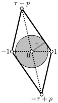
Figure 14.1. Parallelogram $P$ of Lemma 14.1 for $q=5$ and $p=1$.

Proof.

We can assume $p=1$, since the other situation ($p=-1$) is just mirrored. First, we calculate the difference of the areas of the two triangles with vertices $\tau-1$, $-\frac{1}{2}$, $1$ and $\tau-1$, $-\frac{1}{2}$, $0$ and get

$$\tfrac{1}{2}\mathop{{\operatorname{Im}}\thinspace\negthinspace}\mathchoice{\negthinspace}{\negthinspace}{}{}\left({\tau}\right)\left(\tfrac{3}{2}-\tfrac{1}{2}\right)=\tfrac{1}{2}\sqrt{q-\tfrac{1}{4}}.$$

This area is equal to the area of the triangle with vertices $0$, $1$ and $\tau-1$, which is

$$\tfrac{1}{2}s\sqrt{\mathop{{\operatorname{Im}}\thinspace\negthinspace}\mathchoice{\negthinspace}{\negthinspace}{}{}\left({\tau}\right)^{2}+\tfrac{9}{4}}=\tfrac{1}{2}s\sqrt{q+2}.$$

Therefore the desired $s$ follows. ∎

Lemma 14.2.

Let $z$ be in the rectangle $R_{w}$. Then there exists a

$$\Delta\in\left\{{-1,1,\tau-p,-\tau+p}\right\},$$

such that $z-\Delta$ is in the interior of the scaled Voronoi cell $\tau^{w}V$.

Note that we will have $A=z-\Delta$ and $z=\tau C$ in the construction of our expansions. Moreover, the point $z$ is the point inside the rectangle $R_{w}$ whose existence was shown as the main result of Part II, Proposition 5.1.

Proof of Lemma 14.2.

Let $P_{z}$ be the parallelogram with vertices $z+1$, $z+\tau-p$, $z-1$, $z-\tau+p$, i.e., a shifted version of the parallelogram $P$ of Lemma 14.1, see also Figure 14.1. Since $z$ is in the (open) rectangle $R_{w}$, its distance to the line $L$ from $\tau^{w}v_{0}$ to $\tau^{w}v_{1}$ is smaller than $s$ (note that $s$ is the height of the rectangle $R_{w}$, Section 3). Further, since the rectangle $R_{w}$ starts $\sqrt{q}$ away from the points $\tau^{w}v_{0}$ and $\tau^{w}v_{1}$ respectively, the distance from $z$ to one of those two points is larger than $\sqrt{q}$. Therefore, the line $L$ cuts the parallelogram $P_{z}$ into two parts. The two cutting points are on different edges of $P_{z}$. This means, that there exists a vertex of the parallelogram $P_{z}$ on that side of the line $L$, where there is no rectangle $R_{w}$. Such a point lies in the interior of the Voronoi cell $\tau^{w}V$, which can be seen using some properties of $\tau^{w}V$, including that two neighbouring edges of $\tau^{w}V$ have an obtuse angle at their point of intersection and that a disc with center $0$ and radius $\sqrt{q}$ is contained in $\tau^{w}V$. ∎

15. Change in least significant digit

For our construction of the counterexample, we also have to deal with the change in the least significant digit, i.e., with the digits $B$, $D$ and $G$ in the expansions (11.1).

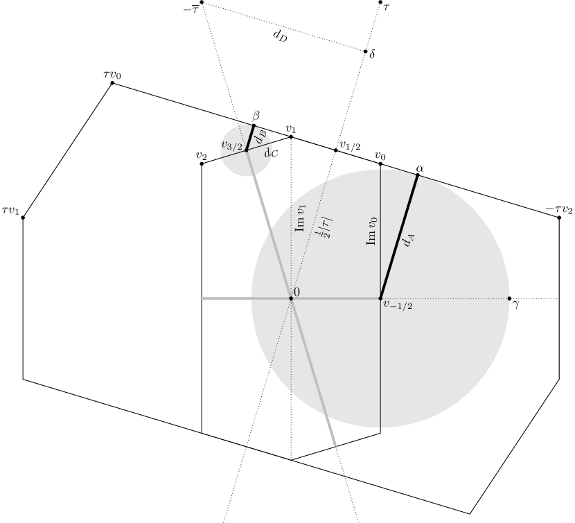
Figure 15.1. Distances and points used in Lemma 15.1 and Proposition 15.3.

Lemma 15.1.

We get

$$d_{A}=\frac{\sqrt{q}}{2}-\frac{1}{4\sqrt{q}}$$

and

$$d_{B}=\frac{1}{4\sqrt{q}}$$

in Figure 15.1.

Proof.

The triangle $v_{-1/2}\alpha v_{0}$ is similar to the triangle $0v_{1/2}v_{1}$. Therefore

$$d_{A}=\mathop{{\operatorname{Im}}\thinspace\negthinspace}\mathchoice{\negthinspace}{\negthinspace}{}{}\left({*}\right){v_{0}}\frac{\frac{1}{2}\left\lvert{\tau}\right\rvert}{\mathop{{\operatorname{Im}}\thinspace\negthinspace}\mathchoice{\negthinspace}{\negthinspace}{}{}\left({*}\right){v_{1}}}=\frac{q-\frac{1}{2}}{2q}\sqrt{q}=\frac{\sqrt{q}}{2}-\frac{1}{4\sqrt{q}}.$$

To calculate $d_{B}$ we start as above. The triangle $v_{3/2}\beta v_{1}$ is similar to the triangle $-\overline{\tau}\delta 0$, so $d_{B}=d_{D}d_{C}/\left\lvert{-\overline{\tau}}\right\rvert$. We have

$$d_{C}=\frac{1}{2}\sqrt{\left(\mathop{{\operatorname{Im}}\thinspace\negthinspace}\mathchoice{\negthinspace}{\negthinspace}{}{}\left({*}\right){v_{1}}-\mathop{{\operatorname{Im}}\thinspace\negthinspace}\mathchoice{\negthinspace}{\negthinspace}{}{}\left({*}\right){v_{2}}\right)^{2}+\left(\frac{1}{2}\right)^{2}}=\frac{1}{2}\sqrt{\frac{1}{4}+\frac{1}{16(q-\frac{1}{4})}}=\frac{1}{4}\sqrt{1+\frac{1}{4q-1}}$$

by the Pythagorean theorem. The distance $d_{D}$ is the projection of $-\overline{\tau}$ on the normalized vector with direction $i\tau$. Therefore

$$d_{D}=\mathop{{\operatorname{Re}}\thinspace\negthinspace}\mathchoice{\negthinspace}{\negthinspace}{}{}\left({\overline{-\overline{\tau}}i\frac{\tau}{\left\lvert{\tau}\right\rvert}}\right)=-\frac{1}{\left\lvert{\tau}\right\rvert}\mathop{{\operatorname{Re}}\thinspace\negthinspace}\mathchoice{\negthinspace}{\negthinspace}{}{}\left({i\tau^{2}}\right)=\frac{1}{\left\lvert{\tau}\right\rvert}\mathop{{\operatorname{Im}}\thinspace\negthinspace}\mathchoice{\negthinspace}{\negthinspace}{}{}\left({\tau^{2}}\right)=\frac{1}{\sqrt{q}}\frac{1}{2}\sqrt{4q-1}=\sqrt{1-\frac{1}{4q}}.$$

Now we can calculate $d_{B}$ as

$$d_{B}=\frac{1}{\sqrt{q}}\sqrt{1-\frac{1}{4q}}\frac{1}{4}\sqrt{1+\frac{1}{4q-1}}=\frac{1}{4\sqrt{q}}.$$

∎

Lemma 15.2.

For each point in $z\in\mathbbm{C}$ there is a lattice point $u\in\mathbbm{Z}[\tau]$ not divisible by $\tau$ with

$$\left\lvert{z-u}\right\rvert<\tfrac{1}{2}\!\left\lvert{\tau}\right\rvert+1=\tfrac{1}{2}\sqrt{q}+1$$

Proof.

First note that if $\eta\in\mathbbm{Z}[\tau]$ is divisible by $\tau$, then $\eta+1$ and $\eta-1$ are not divisible by $\tau$. Consider the lines $z(z+\tau/2)$ and $z(z-\tau/2)$. One of these lines cuts a horizontal line with lattice points $\eta_{k}=j\tau+k$, for some fixed $j\in\mathbbm{Z}$ and all $k\in\mathbbm{Z}$, on it. This means that a lattice point $u$ can be found by first going from $z$ at most a distance of $\left\lvert{\tau}\right\rvert/2$ and then at most $1$ on the horizontal line. Strictly smaller holds since both directions are linearly independent. ∎

Proposition 15.3.

If either $w\geq 4$ and $q\geq 11$ or $w\geq 8$, then there is a possible compensate change.

More precisely, if $w\geq 5$ or $q\geq 5$, then there is a digit $a$ such that $a+\tau^{w-1}$ is a digit as well. If either $w\geq 4$ and $q\geq 11$ or $w\geq 8$, then there is a digit $b$ such that $b+\overline{\tau}\tau^{w-1}$ is a digit as well.

Proof.

The digit set $\mathcal{D}$ is contained in $\tau^{w}V$. Consider the line form $\tau^{w-1}v_{-1/2}=\frac{1}{2}\tau^{w-1}$ to $-\tau^{w-1}v_{-1/2}=-\frac{1}{2}\tau^{w-1}$. From each end point of that line there is a lattice point not divisible by $\tau$ within a radius $\sqrt{q}/2+1$ by Lemma 15.2. With the quantities of Lemma 15.1 one can easily check that the inequality

$$\frac{1}{2}\sqrt{q}+1<\left\lvert{\tau}\right\rvert^{w}\frac{d_{A}}{\left\lvert{\tau}\right\rvert}=\sqrt{q}^{w-1}\left(\frac{\sqrt{q}}{2}-\frac{1}{4\sqrt{q}}\right)$$

holds for either $w\geq 5$ or $q\geq 5$ (fixing $w=2$ makes it easy to check the inequality for $q\geq 5$, then use monotonicity in $w$; use the same argumentation starting with $q=2$ and $w\geq 5$). Thus, the lattice points found above are in the interior of $\tau^{w}V$, and so are our desired digits $a$ and $a+\tau^{w-1}$.

Now we do similarly to get digits $b$ and $b+\overline{\tau}\tau^{w-1}$. We consider the line from $\tau^{w-1}v_{3/2}=-\frac{\overline{\tau}}{2}\tau^{w-1}$ to $-\tau^{w-1}v_{3/2}=-\frac{\overline{\tau}}{2}\tau^{w-1}$ and have to check the inequality

$$\frac{1}{2}\sqrt{q}+1<\left\lvert{\tau}\right\rvert^{w}\frac{d_{B}}{\left\lvert{\tau}\right\rvert}=\sqrt{q}^{w-1}\frac{1}{4\sqrt{q}}.$$

That inequality is satisfied either if $w\geq 4$ and $q\geq 11$ or if $w\geq 8$, which can again be checked easily by monotonicity arguments. For $w=2$ or $w=3$ the inequality is never satisfied. ∎

16. Finding a non-optimal $w$-NAF

In contrast to Section 13, where we have given an explicit construction for a counterexample to minimality of the $w$-NAF, we use a different approach here. It still builds up on the ideas mentioned in the introduction of Part III, i.e., for our construction we consider an element

$$z=A\tau^{w-1}+B\in\mathbbm{Z}[\tau]$$

with nonzero digits $A\in\mathcal{D}$ and $B\in\mathcal{D}$ with the following additional properties. We want to find a change $\Delta$ with

• $\tau\mathbin{\mid}(A+\Delta)$,

• $\tau^{2}\mathbin{\nmid}(A+\Delta)$,

• $\tau^{-1}(A+\Delta)\not\in\mathcal{D}$ and

• $B-\Delta\tau^{w-1}\in\mathcal{D}$.

We will restrict ourselves here to

$$\Delta\in\left\{{-1,1,\tau-p,-\tau+p}\right\},$$

which turns out to be a good choice. (Note that this restriction was already used in Section 14; we only will relax it in Proposition 17.1)

Then the $w$-NAF-expansion of $C=\tau^{-1}(A+\Delta)$ has weight at least $2$, because it (its value) is not a digit. We obtain

$$z=A\tau^{w-1}+B=C\tau^{w}+\left(B-\Delta\tau^{w-1}\right),$$

which shows that $z$ has a (non-$w$-NAF) expansion with weight $2$ and a $w$-NAF-expansion with weight at least $3$. For all of our cases, the right hand side of the previous equation can be rewritten in an expansion

$$z=E\tau^{2w}+F\tau^{w}+G$$

with some digits $E$, $F$ and $G=D=B-\Delta\tau^{w-1}$.

The finding of a point $A+\Delta$ is based on the main result of Part II, $A$ and $\Delta$ are discussed in Section 14, and Section 15 is devoted to get digits $B$ and $G=D$. We just have to glue all the results together, which is done in the proposition below and in the next section. Alternatively, a direct search can be used to find those lattice point configurations; we use this when Part II does not provide a result.

Proposition 16.1.

Suppose either $w\geq 4$ and $q\geq 11$ or $w\geq 8$ (as in Proposition 15.3). Moreover, set

$$C=\tau^{-1}\left(a\tau+b(q-p\tau)\right)$$

and suppose we have

$$\tau C\in R_{w}$$

for some $a\in\mathbbm{Z}$ with $q\mathbin{\nmid}a$ and $b\in\mathbbm{Z}$. Then there exist digits $A$, $B$ and $D$ such that

$$A\tau^{w-1}+B=C\tau^{w}+D.$$

Note that $C$ cannot be a digit because of the following reasons. The point $\tau C$ lies in the rectangle $R_{w}$, and thus $C$ is outside of $\tau^{w}V$, see also Remark 3.1. Since $C$ not divisible by $\tau$ (because $q\mathbin{\nmid}\ell$) either, it has an expansion of weight at least $2$. Using this expansion leads to our desired counterexample.

Proof.

Consider the lattice point $\tau C\in R_{w}$. By Lemma 14.2 there exists a $\Delta\in\left\{{-1,1,\tau-p,-\tau+p}\right\}$ such that

$$A=\tau C-\Delta$$

lies in the interior of the scaled Voronoi cell $\tau^{w}V$. Since $C$ is a lattice point (and $\Delta$ is not divisible by $\tau$), the lattice point $A$ is not divisible by $\tau$. Therefore $A$ is a digit (see Section 12).

Proposition 15.3 gives us the digits $B$ and $D=B-\Delta\tau^{w-1}$. This completes the proof. ∎

17. Collecting all Results

In this final section, we prove the Theorems 2.3 and 2.4 and Proposition 2.5.

Proof of Theorem 2.3.

If we have a lattice point $\tau C\in R_{w}$ not divisible by $\tau^{2}$, then we are able to construct a counterexample by Proposition 16.1. Fortunately Proposition 9.6 provides the explicitly computable bound $w_{q}$ and that for all $w\geq w_{q}$ a $\tau C$ as above exists. ∎

Before proving Theorem 2.4 we need to consider one special case first.

Proposition 17.1.

Let $q=4$ and $p\in\left\{{-1,1}\right\}$ and $w=6$. Set

$$E =1,$$

$$A =7\tau-66p, F =-16p\tau+10,$$

$$B =-65, G =10p\tau-9.$$

Then

$$A\tau^{5}+B=E\tau^{12}+F\tau^{6}+G$$ (17.1)

and both sides of the equation are valid digit expansions, i.e., the $6$-NAF is not a minimal digit expansion.

Proof.

We use a direct search following the same ideas as presented above (especially in Section 16). However, we have to relax our conditions on $\Delta$, in particular, we use $\Delta=-2p$. Moreover, we have $C=17p\tau-10$ as intermediate result in the construction. ∎

Proof of Proposition 2.5 and Theorem 2.4.

We start as in the proof of Theorem 2.3, i.e., we need a lattice point $\tau C\in R_{w}$ not divisible by $\tau^{2}$. The main result of Part II, namely Proposition 5.1, provides the existence of such a lattice point for a fixed $q$ with finitely many (only a few) exceptional values for $w$. For these exceptions, we perform a direct search over all possible lattice points to get $\tau C$ (not lying inside $R_{w}$) and construct the counterexample as described in Section 16. Note that a possible compensate change (Section 15) can be found by a lattice search as well.

This construction of the actual counterexample and lattice search for the exceptions extends Algorithm 10.1; thus completes the proof of Proposition 2.5.

Applying this algorithm, the existence of counterexamples for all $w\geq 4$ is shown; the only exceptions are $q=4$, $p\in\left\{{-1,1}\right\}$ and $w=6$ which are handled separately by Proposition 17.1.

Non-minimality of the cases $w=2$ and $w=3$ (and arbitrary $q\geq 3$) is proven in Section 13. Minimality for $q=2$ and $w\in\left\{{2,3}\right\}$ is shown in [2, 3, 8]. This finishes the proof of Theorem 2.4. ∎

References

- [1] Roberto Avanzi, A note on the signed sliding window integer recoding and a left-to-right analogue, Selected Areas in Cryptography: 11th International Workshop, SAC 2004, Waterloo, Canada, August 9-10, 2004, Revised Selected Papers (H. Handschuh and A. Hasan, eds.), Lecture Notes in Comput. Sci., vol. 3357, Springer-Verlag, Berlin, 2005, pp. 130–143.
- [2] Roberto Avanzi, Clemens Heuberger, and Helmut Prodinger, Minimality of the Hamming weight of the -NAF for Koblitz curves and improved combination with point halving, Selected Areas in Cryptography: 12th International Workshop, SAC 2005, Kingston, ON, Canada, August 11–12, 2005, Revised Selected Papers (B. Preneel and S. Tavares, eds.), Lecture Notes in Comput. Sci., vol. 3897, Springer, Berlin, 2006, pp. 332–344.
- [3] by same author, Scalar multiplication on Koblitz curves. Using the Frobenius endomorphism and its combination with point halving: Extensions and mathematical analysis, Algorithmica 46 (2006), 249–270.
- [4] by same author, Redundant -adic expansions I: Non-adjacent digit sets and their applications to scalar multiplication, Des. Codes Cryptogr. 58 (2011), 173–202.
- [5] Alan Baker and Harold Davenport, The equations and , Quart. J. Math. Oxford 20 (1969), 129–137.
- [6] Ian F. Blake, Gadiel Seroussi, and Nigel P. Smart, Elliptic curves in cryptography, London Mathematical Society Lecture Note Series, vol. 265, Cambridge University Press, 1999.
- [7] John W. S. Cassels, An introduction to the geometry of numbers, Die Grundlehren der mathematischen Wissenschaften in Einzeldarstellungen mit besonderer Berücksichtigung der Anwendungsgebiete, Bd. 99 Springer-Verlag, Berlin-Göttingen-Heidelberg, 1959.
- [8] Daniel M. Gordon, A survey of fast exponentiation methods, J. Algorithms 27 (1998), 129–146.
- [9] Clemens Heuberger, Redundant -adic expansions II: Non-optimality and chaotic behaviour, Math. Comput. Sci. 3 (2010), 141–157.
- [10] Clemens Heuberger and Daniel Krenn, Analysis of width- non-adjacent forms to imaginary quadratic bases, J. Number Theory 133 (2013), no. 5, 1752–1808.
- [11] by same author, Existence and optimality of -non-adjacent forms with an algebraic integer base, Acta Math. Hungar. 140 (2013), no. 1–2, 90–104.
- [12] by same author, Optimality of the width- non-adjacent form: General characterisation and the case of imaginary quadratic bases, J. Théor. Nombres Bordeaux 25 (2013), no. 2, 353–386.
- [13] Jonathan Jedwab and Chris J. Mitchell, Minimum weight modified signed-digit representations and fast exponentiation, Electron. Lett. 25 (1989), 1171–1172.
- [14] Neal Koblitz, CM-curves with good cryptographic properties, Advances in cryptology—CRYPTO ’91 (Santa Barbara, CA, 1991) (J. Feigenbaum, ed.), Lecture Notes in Comput. Sci., vol. 576, Springer, Berlin, 1992, pp. 279–287.
- [15] by same author, An elliptic curve implementation of the finite field digital signature algorithm, Advances in cryptology—CRYPTO ’98 (Santa Barbara, CA, 1998), Lecture Notes in Comput. Sci., vol. 1462, Springer, Berlin, 1998, pp. 327–337.
- [16] Eugene M. Matveev, An explicit lower bound for a homogeneous rational linear form in logarithms of algebraic numbers. II, Izv. Ross. Akad. Nauk Ser. Mat. 64 (2000), no. 6, 125–180.
- [17] Willi Meier and Othmar Staffelbach, Efficient multiplication on certain nonsupersingular elliptic curves, Advances in cryptology—CRYPTO ’92 (Santa Barbara, CA, 1992) (Ernest F. Brickell, ed.), Lecture Notes in Comput. Sci., vol. 740, Springer, Berlin, 1993, pp. 333–344.
- [18] Atsuko Miyaji, Takatoshi Ono, and Henri Cohen, Efficient elliptic curve exponentiation, Information and communications security. 1st international conference, ICICS ’97, Beijing, China, November 11–14, 1997. Proceedings (Yongfei Han, Tatsuaki Okamoto, and Sihan Qing, eds.), Lecture Notes in Comput. Sci., vol. 1334, Springer-Verlag, 1997, pp. 282–290.
- [19] James A. Muir and Douglas R. Stinson, Minimality and other properties of the width- nonadjacent form, Math. Comp. 75 (2006), 369–384.
- [20] Attila Pethö and Benjamin M. M. de Weger, Products of prime powers in binary recurrence sequences. I. The hyperbolic case, with an application to the generalized Ramanujan-Nagell equation, Math. Comp. 47 (1986), no. 176, 713–727.
- [21] Braden Phillips and Neil Burgess, Minimal weight digit set conversions, IEEE Trans. Comput. 53 (2004), 666–677.
- [22] George W. Reitwiesner, Binary arithmetic, Advances in Computers, Vol. 1, Academic Press, New York, 1960, pp. 231–308.
- [23] Paulo Ribenboim, Classical theory of algebraic numbers, Universitext, Springer-Verlag, New York, 2001.
- [24] The SageMath Developers, SageMath Mathematics Software (Version 7.0), 2016, http://www.sagemath.org.
- [25] Jerome A. Solinas, An improved algorithm for arithmetic on a family of elliptic curves, Advances in Cryptology — CRYPTO ’97. 17th annual international cryptology conference. Santa Barbara, CA, USA. August 17–21, 1997. Proceedings (B. S. Kaliski, jun., ed.), Lecture Notes in Comput. Sci., vol. 1294, Springer, Berlin, 1997, pp. 357–371.
- [26] by same author, Efficient arithmetic on Koblitz curves, Des. Codes Cryptogr. 19 (2000), 195–249.