The Barcelona-Catania-Paris-Madrid functional with a realistic effective mass

Abstract

The Barcelona-Catania-Paris-Madrid (BCPM) functional recently proposed to describe nuclear structure properties of finite nuclei is generalized as to include a realistic effective mass. The resulting functional is as good as the previous one in describing binding energies, radii, deformation properties, etc and, in addition, the description of Giant Quadrupole Resonance energies is greatly improved.

I Introduction

In a recent paper BCPM , we developed an energy density functional theory for finite nuclei inspired in the Kohn Sham approach where the bulk part was fitted to the microscopic results of Baldo et al Bal10 . They were obtained with the Brueckner Hartree-Fock (BHF) approach including a three body force taken from Ref Akm98 . The interaction term of the equations of state (EOS) for symmetric nuclear and pure neutron matters were represented by polynomials of even powers in the density supplemented by a quadratic interpolation for asymmetric matter. In this way, a very faithful representation of the microscopic energy per particle $E(\rho_{p},\rho_{n})/A$ as a function of proton (p) and neutron (n) densities was obtained for densities up to about three times saturation density ($\rho_{0}$).

In order to account for finite nuclei, a very simple Hartree type of term was added with a single Gaussian as effective central two body force. Its strength was fixed from the second order term of the polynomial fit and, thus, only one free parameter, the range, was left for adjustment. A second adjustable parameter was given by the strength $W_{\mathrm{LS}}$ of the spin-orbit force which was not extracted from the microscopic calculation though, in principle, this might be possible Sch76 ; Koh12 ; Fuj00 . A third parameter came from the fact that the microscopic equilibrium value of the energy per particle had to be slightly renormalised by about 10^-2 percent because in finite nuclei this value gets coupled with the surface energy. In this case, all coefficients of the polynomials in $\rho_{n},\rho_{p}$ have then been changed by the same factor. With only those three adjustable parameters, namely $r_{0}$, $W_{\mathrm{LS}}$ and $E/A$ of the infinite system, the rms deviation from experimental masses and charge radii were 1.58 MeV and 0.027 fm, respectively BCPM . An analogous procedure for constructing the functional was followed in Ref Fay98 . A variant of this approach was adopted in Ref Cao06 , where a Skyrme force was derived from BHF calculations in nuclear matter, rather than directly the functional. A peculiarity of the BCPM functional is that, like in Ref Fay98 but contrary to most of the Skyrme functionals, its effective mass $m^{*}$ is equal to the bare one $m=m^{*}$. The question of effective mass is a quite subtle one. In principle there are two types of effective masses, the so-called $k$-mass and the $\omega$-mass Jeu76 . The $k$-mass stems from the non locality and, thus, from the momentum ($k$) dependence of the static Hartree-Fock type of mean field which, to fix the ideas, may be derived from a Bruckner $G$-matrix BGM . A typical value of the effective $k$-mass is $m^{*}=0.7m$. On the other hand the so-called $\omega$-mass is obtained in considering dynamic corrections to the single particle self energy which lead to an energy ($\hbar\omega$) dependence. Most of the time a coupling of the single particle motion to higher configurations or to collective modes is considered Jeu76 and this compensates to a large percentage the reduction of the $k$-mass with respect to the bare mass, so that the combined effect is that the total effective mass becomes close to the bare mass again. This effect, however, only holds for the states close to the Fermi energy whereas in the calculation of the ground state energy all configurations enter, so that a precise decision of whether one should take a reduced effective mass or not is difficult to make unless one really undertakes a reliable microscopic calculation for the $\omega$-mass and includes it in the self-consistent mean field cycle. This, however, tremendously complicates the whole approach. Anyway, it seems to be a fact that EDF’s with or without reduced masses are about equally successful and it must be concluded that apparently the ambiguity of the effective mass can be very efficiently mocked up by a renormalisation of finite size properties such as, e.g., the surface energy. On the other hand, for excited states the story can be different. There, not only the $\omega$-mass may be important in considering the propagation of a p-h configuration but collective modes can also be exchanged between the particle and the hole leading to a vertex correction. However, for monopole and isovector giant resonances $\omega$-mass and vertex corrections cancel to a large extent, see the review Ber.83 so that, again, for these modes a bare mass can be taken in ph RPA calculations. The situation is different for higher multipoles where this cancellation does not take place or only to a much smaller extent.

It is our intention in this work to extend our BCPM-EDF to include an effective density dependent mass which we extract again from the same $G$-matrix calculations Bal04 ; Bal10 as it was done for the ground state energy. Also for proton and neutron effective masses we will adjust a polynomial fit in the density. The number of open parameters will stay the same is in the original BCPM-EDF. We shall call the new EDF BCPM^∗.

The paper is organized as follows, in Section II the methodology used to introduce a non-constant effective mass in the BCPM functional is presented along with details on the calculation of finite nuclei. In Section III we present the results of the fit of the new functional to the rms deviation of binding energies. With the new set of parameters we have performed some nuclear structure calculations, like the evaluation of potential energy surfaces relevant to fission and the estimation of the excitation energies of Giant Monopole and Giant Quadrupole resonances.

II Methods

The BCPM energy density functional derived in Ref. BCPM is inspired by the Kohn-Sham density functional theory KS . Although the original KS theory is local, it has been extended to the non-local case, i.e. including effective mass and spin-orbit contributions (see Ref. STV03 and references therein). It uses a simple polynomial of the density $\rho$ and the isospin asymmetry parameter $\beta$ to fit the realistic equation of state of symmetric and neutron matters obtained with a state of the art microscopic calculation with realistic forces. We use the same polynomial for finite nuclei but this time in powers of the density of the finite nucleus

$$\rho(\vec{r})=\sum_{ij}\phi^{*}_{i}(\vec{r})\rho_{ij}\phi_{j}(\vec{r})$$ (1)

Here the $\phi_{i}(\vec{r})$ are some basis wave functions (in our case, harmonic oscillator wave functions) and $\rho_{ij}$ is the density matrix. To incorporate other effects not present or difficult to address in nuclear matter like the spin-orbit interaction or surface energy repulsion, additional terms discussed below are incorporated into the functional. The kinetic energy is treated at the quantum mechanical level by introducing the kinetic energy density

$$\tau(\vec{r})=\sum_{ij}\vec{\nabla}\phi^{*}_{i}(\vec{r})\rho_{ji}\vec{\nabla}\phi_{j}(\vec{r}).$$ (2)

The total energy of a finite nucleus is then given by

$$E=T+E_{int}^{\infty}+E_{int}^{FR}+E_{s.o}+E_{C},$$ (3)

where $T$ is the kinetic energy,

$$E_{int}^{\infty}=\int d\vec{r}\rho(\vec{r})\big{[}P_{s}(\vec{r})(1-\beta^{2}(\vec{r}))+P_{n}(\vec{r})\beta^{2}(\vec{r})\big{]},$$ (4)

is the bulk energy, given in terms of the polynomials $P_{s}(\rho)$ and $P_{n}(\rho)$ for symmetric and neutron matter and the asymmetry density $\beta(\vec{r})=(\rho_{n}(\vec{r})-\rho_{p}(\vec{r}))/\rho(\vec{r})$, $E_{int}^{FR}$ is a finite range surface term, $E_{s.o.}$ is the spin- orbit energy taken from the Skyrme or Gogny forces and $E_{C}$ is the standard Coulomb repulsion including the exchange energy in the Slater approximation. This energy is supplemented by a density-dependent zero range pairing interaction and some beyond mean-field corrections (see again ref. BCPM for details).

The inclusion of an effective mass in BCPM is carried out by means of adding and subtracting an appropriate kinetic energy term to the original kinetic energy density

$$\frac{\hbar^{2}}{2m}\tau\rightarrow\frac{\hbar^{2}}{2m^{*}}\tau+\frac{\hbar^{2}}{2m}\left[1-\left(\frac{m}{m^{*}}\right)\right]\tau^{\infty}.$$ (5)

In this expression $m^{*}$ is the coordinate dependent effective mass, $\tau$ is the quantum kinetic energy density of Eq. (2), and $\tau^{\infty}$ is the semiclassical kinetic energy $\tau^{\infty}=\frac{3}{5}(3\pi^{2})^{2/3}\rho^{5/3}(\vec{r})$. This substitution guarantees that the kinetic energy at nuclear matter level remains the same as before. For simplicity, no explicit mention of isospin is made in the previous formulas, but different effective masses for protons and neutrons are considered. With this redefinition of the kinetic energy the functional now reads

$$E=T^{*}+E_{int}^{\infty\,*}+E_{int}^{FR}+E_{s.o}+E_{C},$$ (6)

where

$$T^{*}=\sum_{\tau}\int d\vec{r}\frac{\hbar^{2}}{2m^{*}_{\tau}}\tau_{\tau}(\vec{r}),$$ (7)

and $E_{int}^{\infty\,*}$ is obtained by adding

$$\frac{\hbar^{2}}{2m}\sum_{\tau}\int d\vec{r}\left[1-\left(\frac{m}{m^{*}_{\tau}}\right)\right]\tau^{\infty}_{\tau}$$ (8)

to $E_{int}^{\infty}$. The rationale behind this procedure is to preserve the nuclear matter EoS of BCPM and, therefore, all the nuclear matter parameters of this functional – see BCPM for a discussion.

Pairing correlations, required to describe open shell nuclei, are introduced by means of a density-dependent zero-range force of the type suggested by Bertsch and Esbenssen ber91 . This force is widely used in nuclear structure calculations gar99 ; baldo08 ; baldo10 . The pairing strength parameters are taken again from gar99 . However in this work we choose the set of values corresponding to an efective mass different from the bare mass. The two-body kinetic energy correction, which accounts for the lack of traslational invariance, is taken as in BCPM . The final ingredient of the energy is the rotational energy correction $\epsilon_{\mathrm{rot}}=\frac{\langle\vec{J}^{2}\rangle}{2\mathcal{J}_{Y}}$ which is subtracted from the functional’s energy. The rotational correction is defined in terms of the Yoccoz moment of inertia Ring.80 and computed using the HFB like intrinsic wave function corresponding to the minimum of the HFB energy. This procedure corresponds to the projection after variation (PAV) method applied to rotational symmetry restoration – see Ring.80 ; RRG00 ; egido04 for a thorough explanation. Note that the rotational energy correction plays an important role in deformed nuclei and its inclusion is relevant to describe masses along the whole periodic table. In strongly deformed mid-shell heavy nuclei the rotational energy correction can reach values as large as 6 or 7 MeV. This correction, however, is almost negligible in magic or semi-magic nuclei, which are basically spherical. Due to the fact that the spherical-deformed transition is sharp, the rotational correction goes from zero to some MeV at the transition point leading to sharp variations in the binding energy plot – see below.

The finite nuclei calculations have been carried out preserving axial symmetry and using an adaptation of the computer code HFBaxial HFBaxial ; rob11 . The quasiparticle operators are expanded in a harmonic oscillator basis with varying number of oscillator shells depending on mass number as to guarantee a weak dependence of binding energies with the basis size – see BCPM for details. In BCPM we have used a simple formula to extrapolate binding energies to the value corresponding to an infinite size HO basis. As this procedure has proven to lead to some difficulties, we have preferred to increase the maximum basis size by adding two major shells, avoiding in this way the infinite basis extrapolation.

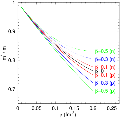
Figure 1: Proton (p, full line) and neutron (n, dotted line) effective masses corresponding to the linear fit of Eq. (10) are plotted as a function of the density for different values of the isospin asymmetry parameter $\beta$.

The effective masses $m^{*}_{n}$ and $m^{*}_{p}$ for neutrons and protons are obtained in the uniform system in terms of the neutron and proton single particle potentials $U_{n}$ and $U_{p}$, calculated within the Brueckner Hartree Fock (BHF) procedure. At the Fermi momenta $k_{Fq}$ one has

$$\frac{m_{q}}{m^{*}_{q}}\,=\,1\,+\,\frac{m_{q}}{\hbar^{2}k_{Fq}}\,\bigg{(}\frac{dU(k)}{dk}\,\bigg{)}_{k=k_{Fq}}$$ (9)

where $q=n,\,p$ and $m_{q}$ is the bare nucleon mass. The effective mass is a function both of the total density $\rho$ and of the asymmetry $\beta\,=\,(\rho_{n}-\rho_{p})/\rho$.

We used Eq. (9) in a systematic calculation of the neutron and proton effective masses for a set of total densities, ranging from $0$ to $0.2$ fm^-3, and asymmetries $\beta$ from $0$ to $1$. We found that the neutron and proton effective masses can be fitted by a simple polynomial expression

$$\frac{m^{*}_{n}}{m_{n}}\,=\,a_{0}(\rho)\,-\,a_{1}(\rho)\beta\ \ \ \ \ ;\ \ \ \ \frac{m^{*}_{p}}{m_{p}}\,=\,a_{0}(\rho)\,+\,a_{1}(\rho)\beta,$$ (10)

where

$$a_{0} =\,1-1.744025\rho+2.792075\rho^{2}$$

$$a_{1} =\,0.090795\rho+2.981724\rho^{2}.$$ (11)

This expression can be extended to negative values of $\beta$, provided we simply interchange neutrons and protons, as it must be. Since the neutron and proton effective masses have a symmetric splitting, see Eq. (10) and Fig 1, they have a continuous derivative at $\beta=0$. The fit with the linear dependence of $\beta$ looks not enough for the whole range up to $\beta=1$ (pure neutron matter). However a good fit can be obtained up to values of $\beta\approx 0.5$, which are within the range of values appearing in stable nuclei, with the exception of very light nuclei, for which the BCPM functional is not expected to be applicable. Therefore, we keep the fit of Eq. (10,11) neglecting the deviations, which can appear at very large asymmetries. These deviations could be taken into account by introducing higher powers in $\beta$. However this would not be relevant for finite nuclei, and we prefer to keep the simplicity of the linear dependence. We are aware, however, that in situations of large asymmetry like in Wigner-Seitz cells in neutron stars our simple linear dependence would not be enough. The present approach is in line with phenomenological optical model analyses. In ref. Bao1 the neutron to proton mass splitting is expressed as $(m^{*}_{n}-m^{*}_{p})/m=(0.27\pm 0.25)\beta$, while more recently Bao2 a similar analysis gives $(0.41\pm 0.15)\beta$. From Eq. (11) at saturation one finds $0.2\beta$, i.e. a splitting that agrees in the sign but it appears to be on the small side. In any case one should appreciate the rough agreement between phenomenology and theory what is not obvious nor trivial. In finite nuclei the polynomial fit in Eq. (10) is maintained but using the finite nucleus density instead of the nuclear matter one.

III Results

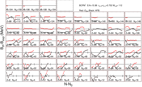
Figure 2: The binding energy difference $\Delta B=B_{\mathrm{th}}-B_{\mathrm{exp}}$ (MeV) is plotted as a function of the shifted (by N₀(Z)) neutron number N-N₀(Z) for all the isotopic chains considered. The values of Z and the neutron number shift N₀(Z) for each chain are given in the corresponding panel. The ordinate $\Delta B$ axis ranges from -5.5 MeV to 5.5 MeV with long ticks every 2 MeV. The N-N₀(Z) axis spans a range of 40 units with long ticks every 10 units and short ones every 1 unit. In every panel, a horizontal line corresponding to $\Delta B=0$ has been plotted to guide the eye. Additional perpendicular lines signaling the position of magic neutron numbers have also been included.

In this section we discuss first the fitting of the free parameters of the BCPM^∗ functional to minimize the root mean square (rms) binding energy difference with the experimental data. The functional so obtained is then used to carry out calculations to asset the merits of the functional regarding quadrupole deformation properties and excitation energies of Giant Resonances.

III.1 Binding energies and radii

As a consequence of the introduction of the effective mass in finite nuclei, a readjustment of the parameters of BCPM is required. The most affected is the spin-orbit interaction strength, which is inversely proportional to the effective mass and, therefore, is going to have a value in BCPM^∗ closer to the value of other functionals like Gogny D1S or D1M with effective masses not equal to the bare one. The reason for such dependence is the link between the spin-orbit strength and the magic numbers: $W_{\mathrm{LS}}$ has to be large enough as to bring intruder orbital down to the lower major shell. Decreasing the effective mass increases the gap between major shells and, therefore, a larger $W_{\mathrm{LS}}$ value is required. The spin-orbit strength along with the other two range parameters $r_{0L}$ and $r_{0U}$ (see BCPM for more information) are readjusted as to fit the binding energies of even-even nuclei in a similar manner as in BCPM . The minimum value of the rms for the binding energy difference using the AME 2012 experimental compilation including 620 even-even nuclei AW.12 is $\sigma_{\mathrm{E}}=1.68\mathrm{MeV}$ which is slightly higher than the original BCPM value of 1.58 MeV obtained with only 579 even-even nuclei (1.61 MeV when the AME 2012 compilation is considered). The values of the fitted parameters are $r_{0U}=r_{0L}=0.752$ fm and $W_{\mathrm{LS}}=112$ MeV. We observe that as in the BCPM case, the minimization of the binding energy favors equal values of the $r_{0U}$ and $r_{0L}$ ranges. In Fig 2 the binding energy difference is plotted as a function of neutron number for the different values of Z (see figure caption for an explanation of the plot). In this plot we observe a nice reproduction of experimental data for heavy nuclei away from magic or semi-magic numbers. Close to magic numbers we observe in many cases a non-smooth behavior which is due, as explained in BCPM , to a deficiency on the way the rotational energy correction used in the binding energy is computed: As mentioned in the previous section, the rotational energy correction is obtained using the projection after variation method where the correction is computed using the intrinsic wave function minimizing the HFB energy and, therefore, it is zero for spherical intrinsic states. The correction suddenly jumps by a couple of MeV when the spherical to deformed transition takes place and the jump obviously reflects in the binding energy. This deficiency could be cured by computing the rotational energy correction in the variation after projection (VAP) scheme but this procedure, even in an approximate way, is much more costly to implement than the used PAV method. Work to find a convenient way to implement the VAP is under way. For light nuclei the agreement with the experimental binding energies deteriorates and the dependence with proton and neutron number is not well reproduced.

Concerning charge radii we have also computed the root mean deviation $\sigma_{R}$ with respect to the 315 experimental points in the recent compilation of Angeli et al angeli04 . The theoretical radius is computed using the standard formula $r_{\mathrm{ch}}=\sqrt{\langle r^{2}\rangle_{\mathrm{HFB}}+0.875^{2}}$. The value obtained for $\sigma_{R}$ using the BCPM^∗ functional is $\sigma_{R}=0.024\mathrm{fm}$, which is around 15% better than the 0.027 fm value obtained with BCPM. In Fig 3 we plot the difference between the theoretical and experimental value of the charge radii as a function of the mass number A for the 315 even-even nuclei with experimentally known charge radii angeli04 . Overall, we see a very good agreement with experimental data, except in some super-heavy and light nuclei. These deficiencies were also observed in the BCPM results of Ref BCPM .

Figure 3: The experiment-theory deviation $r_{\mathrm{ch}}-r_{\mathrm{exp}}$ for the 315 even-even nuclei with known experimental data angeli04 is plotted as a function of mass number A.

As the nuclear matter EoS of BCPM has been preserved in BCPM^∗, all its nuclear matter parameters $K$, $J$, etc remain exactly the same as with BCPM and we refer the reader to Ref BCPM for an extensive discussion of their values. In addition, the BCPM^∗ values of the range parameters of the surface term have not changed substantially, with respect to the ones of BCPM and, therefore, it is to be expected that the variance analysis of $\sigma_{E}$ with respect to the parameters $r_{0L}$, $r_{0U}$ and $W_{\mathrm{LS}}$ carried out in BCPM is going to yield similar conclusions for BCPM^∗.

III.2 Fission barrier heights

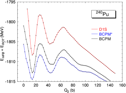
Figure 4: Potential energy surface for fission, including the rotational energy correction, computed as a function of the quadrupole moment (in b) for the Gogny D1S, BCPM and BCPM^∗ functionals.

A fundamental aspect of any nuclear effective interaction is its ability to produce reasonable deformation properties. The fission phenomenon, which is described as the collective evolution of the nucleus from its ground state to scission using the quadrupole deformation parameter as driving coordinate, is perhaps the best testing ground in this respect. From the perspective of comparing with experimental data, there are well established values of the fission barrier heights in a bunch of actinides and super-heavies that could be used. Those values are extracted in a model dependent way from the behavior of the induced fission cross section as a function of the energy and are routinely used as benchmarks of theoretical fission models. In previous studies Giu.13 ; Giu14 we have shown that the BCPM interaction produces quite reasonable results for fission observables. Therefore, we have repeated some of the calculations to evaluate the impact of the effective mass on those observables. In order to obtain barrier heights, the computation of the energy landscape as a function of the quadrupole moment is required. An example of such kind of calculations is shown in Fig 4 using the paradigmatic case of ²⁴⁰Pu. For comparison, the results obtained with BCPM and with the Gogny D1S functional D1S are also plotted. The potential energy is given by the HFB one including the standard rotational energy correction $\langle\Delta\vec{J}^{2}\rangle/(2\mathcal{J}_{\mathrm{Y}})$ Ring.80 . The results for the three functionals show a very similar behavior, with the position of maxima and minima being almost the same in the three cases. It is remarkable to notice the shoulder obtained with both BCPM and BCPM^∗ at $Q_{20}=90\mathrm{b}$ which is reminiscent of a second isomeric well. The connection of this shoulder with the second isomeric well observed in some U and Th isotopes deserves further investigation. The values obtained for the two barrier heights are given in Table 1 along with the corresponding numbers for ²³⁴U and ²⁴⁶Cm and compared with experimental data.

	EA	EB	EI	EA	EB	EI	EA	EB	EI
	BCPM∗			BCPM			Exp
234U	5	5.8	1.8	5.6	5.6	2.	4.8	5.5	–
240Pu	6.2	5.5	1.7	7.3	5.8	2.1	6	5.15	2.8
246Cm	6.5	4.7	1.1	8	5.5	2.1	6	4.8	–

Table 1: First (E_A) and second (E_B) fission barrier heights and the excitation energy of the fission isomer (E_I) are given in MeV for three typical actinide nuclei. Results obtained with BCPM^∗ and BCPM are given along with the experimental data from Ber15 .

We observe that both the results obtained with BCPM^∗ as well as the ones with BCPM are in a quite good agreement with experimental data Ber15 , the ones obtained with BCPM^∗ being slightly better. The results can not be taken as conclusive because triaxiality is not allowed to develop in the first barrier. However, the agreement of the calculations with experimental data for the second barrier is very encouraging as, in this case, triaxiality has proven to play a marginal role. Other observable quantity relevant in fission studies is the excitation energy of the fission isomer E_I which is also given in the Table along with the only existing experimental datum for ²⁴⁰Pu. The theoretical predictions are lower than the experimental value by around 25 % to 40 %, with the BCPM^∗ result lower than the BCPM one and, therefore, slightly worse in terms of the comparison with the experiment.

In the three cases studied, reflection symmetry is broken for quadrupole moments beyond the second fission barrier. The behavior and values of the octupole moment for those configurations are very similar to the ones obtained with BCPM and Gogny D1S, indicating that the good octupole properties of those functionals are preserved in the present proposal. Work to analyze in more detail deformation properties of BCPM^∗ is in progress and will be reported elsewhere.

III.3 Monopole and quadrupole giant resonance energies

Figure 5: Excitation energies of the monopole and quadrupole giant resonances as a function of mass number A obtained with the scaling approximation. The estimation $58A^{-1/3}$ for the quadrupole and $86A^{-1/3}$ for the monopole Ring.80 are drawn to guide the eye. The dotted curve $67A^{-1/3}$ corresponds to the quadrupole’s best fit.

In our previous work we have discussed with some detail the excitation properties of the BCPM energy density functional. In particular, we analyzed the excitation energies of the scalar giant monopole and quadrupole resonances (GMR and GQR, respectively) using sum rule techniques. We found that the BCPM predictions for the excitation energies of the GMR were in agreement with the results provided by other mean field models, non-relativistic and relativistic, with a similar value of the incompressibility modulus $K$. However, it was found that the experimental excitation energies of the GQR were systematically underestimated by about 1 MeV. The underlying reason for that was that in BCPM the effective mass equals the bare one and it is known that the GQR excitation energies are sensitive to the value of the effective mass.

We have repeated these calculations in the present work using the BCPM^∗ energy density functional. In Table 2 we report the theoretical estimates of the excitation energy of the GMR and GQR, computed with our new functional, of a selected set of nuclei, for which the GMR excitation energy is experimentally known.

Comparing with Table VII of BCPM , one can see that the influence of the effective mass on the excitation energy of the GMR is basically negligible, while it is noticeable in the case of the GQR. This behavior can be understood in the scaling approach as follows. The scaled $m_{3}$ sum rules for the GMR and the GQR (see Eqs. (A12) and (A17) of BCPM ) contain a kinetic energy contribution coming from the second derivative of the scaled energy density respect to the scaling parameter $\lambda$. According to the transformation of Eq. 5, used in BCPM^∗ to account for the kinetic energy, it is easy to see that both contributions $\tau$ and $\tau^{\infty}$ scale as $\lambda^{2}$ in the monopole case while in the quadrupole one only $\tau$, given by Eq. 2, contributes as a consequence of volume conservation in the quadrupole oscillation. As far as in BCPM^∗ the effective mass $m^{*}$ is smaller than the bare mass $m$, the $m_{3}$ value and the excitation energy of the GQR $E_{3}(Q)$ will be larger than the predictions of the BCPM functional where $m^{*}=m$. Therefore, the agreement with the experimental values of the excitation energy of the GQR is better when computed with the BCPM^∗ functional, as it can be seen in Table II.

In Figure 5 we display the excitation energies of the monopole and quadrupole oscillations along the whole periodic table. Both follow a $C\,A^{-1/3}$ law with coefficients $C_{M}=86$ and $C_{Q}=67$ MeV, respectively. These values are roughly in agreement with the empirical values given in Ring.80 of 86 and 58 MeV for the monopole and quadrupole resonances.

Table 2: Theoretical $E_{3}$ and $E_{1}$ estimates (in MeV) of the average excitation energy of the GMR including pairing correlations. The $E_{3}$ estimate of the GQR, also including pairing, is also displayed. The experimental energy of the centroid and the corresponding error for the GMR and GQR are also given.

Nucleus	$E_{3}(M)$	$E_{1}(M)$	$E_{3}(Q)$	Exp(M)	Exp(Q)
90Zr	19.10	18.31	14.65	17.81 $\pm$ 0.32	14.30 $\pm$ 0.40
144Sm	16.45	15.66	12.59	15.40 $\pm$ 0.30	12.78 $\pm$ 0.30
208Pb	14.53	13.89	11.18	13.96 $\pm$ 0.20	10.89 $\pm$ 0.30
112Sn	17.73	16.96	13.64	16.1 $\pm$ 0.1	13.4 $\pm$ 0.1
114Sn	17.62	16.85	13.56	15.9 $\pm$ 0.1	13.2 $\pm$ 0.1
116Sn	17.50	16.81	13.48	15.8 $\pm$ 0.1	13.1 $\pm$ 0.1
118Sn	17.39	16.70	13.41	15.6 $\pm$ 0.1	13.1 $\pm$ 0.1
120Sn	17.28	16.59	13.34	15.4 $\pm$ 0.2	12.9 $\pm$ 0.1
122Sn	17.18	16.39	13.28	15.0 $\pm$ 0.2	12.8 $\pm$ 0.1
124Sn	17.08	16.28	13.22	14.8 $\pm$ 0.2	12.6 $\pm$ 0.1
106Cd	18.01	17.16	13.87	16.50 $\pm$ 0.19
110Cd	17.74	16.89	13.68	16.09 $\pm$ 0.15	13.13 $\pm$ 0.66
112Cd	17.61	16.85	13.59	15.72 $\pm$ 0.10
114Cd	17.48	16.65	13.50	15.59 $\pm$ 0.20
116Cd	17.36	16.53	13.42	15.40 $\pm$ 0.12	12.50 $\pm$ 0.66

IV Conclusions

In this work we propose a variant of the BCPM energy density functional published in BCPM , where the bare mass is replaced by a density dependent effective mass $m^{*}$. Though it may not be absolutely clear whether bare or effective mass is preferable as we argued in the Introduction, it is certainly true that for, e.g., giant resonances other than monopole and dipole ones an effective mass $m^{*}<m$ is favored. Again we used our strategy and deduced the effective mass from our microscopic G-matrix results and adjusted separately proton and neutron effective masses to our results of the Bruckner G-matrix using polynomials in the density. A linear interpolation between proton and neutron masses was fitted to the asymmetries prevailing in finite nuclei. It turns out that the difference of both masses is quite a bit on the lower side of what one generally finds in the literature. In finite nuclei the densities are then replaced by the local ones as obtained from the HFB calculation. Some parameters had to be readjusted, in first place this concerns the strength of the spin-orbit term, which now has values much closer to the usual values of Skyrme or Gogny functionals. Concerning the results, not surprisingly, the ones for the giant quadrupole resonance are now in significantly better agreement with experimental data. Fission barriers from BCPM^∗ are slightly better than those with BCPM. On the other hand the excitation energy of the fission isomer is slightly worse for the only data point of ²⁴⁰Pu with BCPM^∗ than BCPM. The rms value for the masses is 1.68 MeV with BCPM^∗ and 1.58 MeV with BCPM, the rms value for the radii is 0.024 fm instead of 0.027 fm. All in all it can be said that BCPM^∗ practically performs as well as BCPM for all quantities besides for the GQR where it yields sensitively better results.

- (1) M. Baldo, L.M. Robledo, P. Schuck and X. Viñas, Phys. Rev. C 87, 064305 (2013).
- (2) M. Baldo, L. Robledo, P. Schuck, X. Viñas, J. Phys. G Nucl. and Part. Physics 37, 064015 (2010) and references there in.
- (3) A. Akmal, V. R. Pandharipande, D. G. Ravenhall, Phys. Rev. C 58, 1804 (1998).
- (4) R. R. Scheerbaum, Nucl. Phys. A 257, 77 (1976).
- (5) M. Kohno, Phys. Rev. C 86, 061301 (2012).
- (6) Y. Fujiwara, M. Kohno, T. Fujita, C. Nakamoto and Y. Suzuki, Nucl. Phys. A 674, 493 (2000).
- (7) S.A. Fayans, JETP Lett. 68, 169 (1998).
- (8) L.G. Cao, U. Lombardo, C.W. Shen and N. V. Giai, Phys. Rev. C 73, 014313 (2006).
- (9) J. P. Jeukenne, A. Lejeune, C. Mahaux, Phys. Rep. 25, 83 (1976).
- (10) M. Baldo, G.F. Burgio, H.-J. Schulze and G. Taranto, Phys. Rev. C89, 048801 (2014).
- (11) G. F. Bertsch, P. F. Bortignon, and R. A. Broglia Rev. Mod. Phys. 55, 287 (1983).
- (12) M.Baldo, C.Maieron, P.Schuck and X.Viñas, Nucl. Phys. A 736, 241 (2004).
- (13) W. Kohn and L.J. Sham, Phys. Rev. 140, A1133 (1965).
- (14) V.B. Soubbotin, V.I. Tselyaev and X. Viñas Phys. Rev. C 67, 014324 (2003).
- (15) G. F. Bertsch and H. Esbensen Ann. Phys. 209 327 (1991).
- (16) E. Garrido, P. Sarriguren, E. Moya de Guerra and P. Schuck Phys. Rev. C 60 064312 (1999).
- (17) Baldo M, Schuck P and Viñas X Phys. Lett. B 663, 390 (2008).
- (18) Baldo M, Robledo L, Schuck P and Viñas X 2010 J. Phys G: Nucl. Part. Phys. 37 064015 (2010).
- (19) P. Ring and P. Schuck, The Nuclear Many Body Problem (Springer–Verlag Edt. Berlin, 1980).
- (20) R. R. Rodríguez-Guzmán, J.L. Egido, and L.M. Robledo Phys. Rev. C 62, 054319 (2000).
- (21) J.L. Egido and L.M. Robledo Lec. Notes in Phys. 641, 269 (2004).
- (22) L.M. Robledo, HFBaxial computer code (2002).
- (23) L.M. Robledo and G.F. Bertsch, Phys. Rev. C 84, 014312 (2011).
- (24) Bao-An Li and Xiao Han, Phys. Lett. B 727, 276 (2013).
- (25) Xiao-Hua Li et al., Phys. Lett. B 743, 4018 (2015).
- (26) M. Wang et al, Chinese Phys. C 36, 1603 (2012).
- (27) Angeli I At. Data Nuc. Data Tables 87 185 (2004).
- (28) J. F. Berger, M. Girod, and D. Gogny, Nucl. Phys. A 428, 23c (1984).
- (29) S.A. Giuliani and L.M Robledo, Phys. Rev. C 88, 054325 (2013).
- (30) S.A. Giuliani, L.M. Robledo and R. Rodríguez-Guzmán Phys Rev C 90, 054311 (2014)
- (31) G.F. Bertsch, W. Loveland, W. Nazarewicz, and P. Talou P J. of Phys. G 42 077001 (2015)