A biobjective approach to robustness based on location planning

Abstract

Finding robust solutions of an optimization problem is an important issue in practice, and various concepts on how to define the robustness of a solution have been suggested. The idea of recoverable robustness requires that a solution can be recovered to a feasible one as soon as the realized scenario becomes known. The usual approach in the literature is to minimize the objective function value of the recovered solution in the nominal or in the worst case.

As the recovery itself is also costly, there is a trade-off between the recovery costs and the solution value obtained; we study both, the recovery costs and the solution value in the worst case in a biobjective setting.

To this end, we assume that the recovery costs can be described by a metric. We demonstrate that this leads to a location planning problem, bringing together two fields of research which have been considered separate so far.

We show how weakly Pareto efficient solutions to this biobjective problem can be computed by minimizing the recovery costs for a fixed worst-case objective function value and present approaches for the case of linear and quasiconvex problems for finite uncertainty sets. We furthermore derive cases in which the size of the uncertainty set can be reduced without changing the set of Pareto efficient solutions.

Keywords

robust optimization; location planning; biobjective optimization

1 Introduction

Robust optimization is a popular paradigm to handle optimization problems contaminated with uncertain data, see, e.g., [BTGN09, ABV09] and references therein.

Starting from conservative robustness models requiring that the robust solution is feasible for any of the possible scenarios, new concepts have been developed, see [GS16] for a recent survey. These concepts allow to relax this conservatism and to control the price of robustness, i.e., the loss of objective function value one has to pay in order to obtain a robust solution, see [BS04]. In many real-world problems these new robustness concepts have been successfully applied.

Motivated by two-stage stochastic programs, one class of such new models includes the so called recoverable robustness introduced in [LLMS09, CDS⁺07] and independently also used in [EMS09]. Recoverable robustness is a two-stage approach that does not require the robust solution to be feasible for all scenarios. Instead, a recoverable-robust solution comes together with a recovery strategy which is able to adapt the solution to make it feasible for every scenario. Such a recovery strategy can be obtained by modifying the values of the solution or by allowing another resource or spending additional budget, as soon as it becomes known which scenario occurs. Unfortunately, a recoverable-robust solution can only be determined efficiently for simple problems with special assumptions on the uncertainties and on the recovery algorithms (see [Sti08]), and the recoverable-robust counterpart is known to be NP-hard even in simple cases [CDS⁺09b].

Our contributions. In this paper we analyze the two main goals in recoverable robustness: Obtaining a good objective function value in the worst case while minimizing the recovery costs. We consider the $\varepsilon$-constrained version as a geometric problem, which allows to interpret robustness as a location planning problem, and derive results on Pareto efficient solutions and how to compute them.

Overview. The remainder of the paper is structured as follows.

In the next section we sketch classic and more recent robustness concepts before we introduce the biobjective version of recoverable robustness in Section 3. We then analyze how to solve the scalarization of the recoverable-robust counterpart in Section 4, and consider reduction approaches in Section 5. After discussing numerical experiments in Section 6, we conclude with a summary of results and an outlook to further research in Section 7.

2 Robustness concepts

2.1 Uncertain optimization problems

We consider optimization problems that can be written in the form

(P) $${\rm minimize}\ f(x)$$

$$\mbox{s.t. }F(x)\leq 0$$

$$x\in\mathcal{X},$$

where $\mathcal{X}\subseteq{\rm IR}^{n}$ is a closed set, $F:{\rm IR}^{n}\to{\rm IR}^{m}$ describes the $m$ constraints and $f:{\rm IR}^{n}\to{\rm IR}$ is the objective function to be minimized. We assume $f$ and $F$ to be continuous. In practice, the constraints and the objective may both depend on parameters which are in many cases not exactly known. In order to accommodate such uncertainties, the following class of problems is considered instead of $\rm(P)$.

Notation 1.

An uncertain optimization problem is given as a parameterized family of optimization problems

P($$\xi {\rm minimize}\ f(x,\xi)$$)

$$\mbox{s.t. }F(x,\xi)\leq 0$$

$$x\in\mathcal{X},$$

where $F(\cdot,\xi):{\rm IR}^{n}\to{\rm IR}^{m}$ and $f(\cdot,\xi):{\rm IR}^{n}\to{\rm IR}$ are continuous functions for any fixed $\xi\in\mathcal{U}$, $\mathcal{U}\subseteq{\rm IR}^{M}$ being the uncertainty set which contains all possible scenarios $\xi\in{\rm IR}^{M}$ which may occur (see also [BTGN09]).

A scenario $\xi\in\mathcal{U}$ fixes the parameters of $f$ and $F$. It is often known that all scenarios that may occur lie within a given uncertainty set $\mathcal{U}$, however, it is not known beforehand which of the scenarios $\xi\in\mathcal{U}$ will be realized. We assume that $\mathcal{U}$ is a closed set in ${\rm IR}^{M}$ containing at least two elements (otherwise, no uncertainty would affect the problem). Contrary to the setting of stochastic optimization problems, we do not assume a probability distribution over the uncertainty set to be known.

The set $\mathcal{X}$ contains constraints which do not depend on the uncertain parameter $\xi$. These may be technological or physical constraints on the variables (e.g., some variables represent non-negative magnitudes, or there are precedence constraints between two events), or may refer to modeling constraints (e.g., some variables are Boolean, and thus they can only take the values 0 and 1).

In short, the uncertain optimization problem corresponding to P($\xi$) is denoted as

$$(\mbox{P($\xi$)},\xi\in\mathcal{U}).$$ (1)

We denote

$$\mathcal{F}(\xi)=\{x\in\mathcal{X}:F(x,\xi)\leq 0\}$$

as the feasible set of scenario $\xi\in\mathcal{U}$ and

$$f^{*}(\xi)=\min\{f(x,\xi):F(x,\xi)\leq 0,x\in\mathcal{X}\}$$

as the optimal objective function value for scenario $\xi$ (which might be $\infty$ if it does not exist). Note that $\mathcal{F}(\xi)$ is closed in ${\rm IR}^{n}$, as we assumed $\mathcal{X}$ to be closed, and $F(\cdot,\xi)$ to be continuous. In the following we demonstrate the usage of $\xi\in{\rm IR}^{M}$ for the case of linear optimization. In the simplest case, $\xi$ coincides with the uncertain parameters of the given optimization problem.

Example 1.

Consider a linear program ${\rm minimize}\{c^{t}x:Ax\leq b,x\in{\rm IR}^{n}\}$ with a coefficient matrix $A\in{\rm IR}^{m,n}$, a right-hand side vector $b\in{\rm IR}^{m}$ and a cost vector $c\in{\rm IR}^{n}$. If $A,b$, and $c$ are treated as uncertain parameters, we write

P($$A,b,c {\rm minimize}\ f(x,(A,b,c))=c^{t}x$$)

$$\mbox{s.t. }F(x,(A,b,c))=Ax-b\leq 0$$

$$x\in\mathcal{X}={\rm IR}^{n},$$

i.e., $\xi=(A,b,c)\in{\rm IR}^{M}$ with $M=n\cdot m+n+m$

However, in (1) we allow a more general setting, namely that the unknown parameters $A,b,c$ may depend on (other) uncertain parameters $\xi\in{\rm IR}^{M}$. For example, there might be $M=1$ parameter $\xi\in{\rm IR}$ which determines all values of $A,b,c$. As an example imagine that the temperature determines the properties of different materials. In such a case we would have

$$f(x,\xi):{\rm IR}^{n}\times{\rm IR}\to{\rm IR},\mbox{ and }$$

$$F(x,\xi):{\rm IR}^{n}\times{\rm IR}\to{\rm IR}^{m},$$

where $f(x,\xi)=c(\xi)^{t}x$ and $F(x,\xi)=A(\xi)x-b(\xi)$.

We now summarize several concepts to handle uncertain optimization problems.

2.2 Strict robustness and less conservative concepts

The first formally introduced robustness concept is called strict robustness here. It has been first mentioned by Soyster [Soy73] and then formalized and analyzed by Ben-Tal, El Ghaoui, and Nemirovski in numerous publications, see [BTGN09] for an extensive collection of results. A solution $x\in\mathcal{X}$ to the uncertain problem (1) is called strictly robust if it is feasible for all scenarios in $\mathcal{U}$, i.e., if $F(x,\xi)\leq 0$ for all $\xi\in\mathcal{U}$. The set of strictly robust solutions with respect to the uncertainty set $\mathcal{U}$ is denoted by ${\rm SR}(\mathcal{U})=\bigcap_{\xi\in\mathcal{U}}\mathcal{F}(\xi)$. The strictly robust counterpart of (1) is given as

$$\mbox{RC}(\mathcal{U})\hskip 28.45274pt {\rm minimize}\ \sup_{\xi\in\mathcal{U}}f(x,\xi)$$

$$\mbox{s.t. }x\in{\rm SR}(\mathcal{U})$$

The objective follows the pessimistic view of minimizing the worst case over all scenarios.

Often the set of strictly robust solutions is empty, or all of the strictly robust solutions lead to undesirable solutions (i.e., with considerably worse objective values than a nominal solution would achieve). Recent concepts of robustness hence try to overcome the “over-conservative” nature of the previous approach. In this paper we deal with recoverable robustness which is described in the next section. Other less conservative approaches include the approach of Bertsimas and Sim [BS04], reliability [BTN00], light robustness [FM09, Sch14], adjustable robustness [BTGGN04] (which will be used in Section 3.3), and comprehensive robustness [BTBN06]. For a more detailed recent overview on different robustness concepts we refer to [GS16].

3 A biobjective approach to recoverable robustness

Our paper extends the recently published concepts of recoverable robustness. As before, we consider a parameterized problem

P($$\xi {\rm minimize}\ f(x,\xi)$$)

$$\mbox{s.t. }F(x,\xi)\leq 0$$

$$x\in\mathcal{X}$$

The idea of recoverable robustness (see [LLMS09]) is to allow that a solution can be recovered to a feasible one for every possible scenario. There, a solution $x\in\mathcal{X}$ is called recoverable-robust if there is a function $y:\mathcal{U}\to\mathcal{X}$ such that for any possible scenario $\xi\in\mathcal{U}$, the solution $y(\xi)\in\mathcal{F}(\xi)$ is not too different from the original solution $x$. This includes on the one hand the costs for changing the solution $x$ to the solution $y(\xi)$, and on the other hand the objective function value of $y(\xi)$ compared to the objective function value of $x$. The solution $y(\xi)$ is called the recovery solution for scenario $\xi$.

Examples include recoverable-robust models for linear programming [Sti08], shunting [CDS⁺07], timetabling [CDS⁺09a], platforming [CGST14], the empty repositioning problem [EMS09], railway rolling stock planning [CCG⁺12] and the knapsack problem [BKK11]. An extensive investigation can be found in [Sti08]. Note that the model has the drawback that even for simple optimization problems an optimal recoverable-robust solution is usually hard to determine.

3.1 Model formulation

Various goals may be followed when computing a recoverable-robust solution: On the one hand, the new solution should be recoverable to a good solution $y(\xi)\in\mathcal{F}(\xi)$ for every scenario $\xi\in\mathcal{U}$. On the other hand, also the costs of the recovery are important: A new solution has to be implemented, and if $x$ differs too much from $y(\xi)$ this might be too costly. We assume that the recovery costs can be measured by a metric $d:{\rm IR}^{n}\times{\rm IR}^{n}\to{\rm IR}$. An example for metric recovery costs can be found, e.g., for shunting in [CCG⁺12]; recovery costs defined by norms are also used frequently, e.g., in timetabling [LLMS09], in recoverable-robust linear programming [Sti08], or in vehicle scheduling problems [GDT15].

Our biobjective model for recoverable robustness can be formulated as follows:

(Rec) $${\rm minimize}\ \left({\bf f}(y),{\bf r}(x,y)\right)=\left(\sup_{\xi\in\mathcal{U}}f(y(\xi),\xi),\sup_{\xi\in\mathcal{U}}d(x,y(\xi))\right)$$

$$\mbox{s.t. }F(y(\xi),\xi)\leq 0\ \ \mbox{ for all }\xi\in\mathcal{U}$$

$$x\in\mathcal{X},y:\mathcal{U}\to\mathcal{X}$$

We look for a recoverable robust solution $x$ together with a recovery solution $y(\xi)\in\mathcal{F}(\xi)$ for every scenario $\xi\in\mathcal{U}$. Note that if $\mathcal{U}$ is infinite, (Rec) is not a finite-dimensional problem. In the objective function we consider

• the quality $f(y(\xi),\xi)$ of the recovery solutions, which will finally be implemented, in the worst case, and

• the costs of the recovery $d(x,y(\xi))$, i.e., changing $x$ to $y(\xi)$, again in the worst case.

As usual in multi-criteria optimization we are interested in finding Pareto efficient solutions to this problem. Recall that a solution $(x\in\mathcal{X},y:\mathcal{U}\to\mathcal{X})$ is weakly Pareto efficient if there does not exist another solution $x^{\prime}\in\mathcal{X},y^{\prime}:\mathcal{U}\to\mathcal{X}$ such that

$$\sup_{\xi\in\mathcal{U}}f(y^{\prime}(\xi),\xi) < \sup_{\xi\in\mathcal{U}}f(y(\xi),\xi)\mbox{ and }$$

$$\sup_{\xi\in\mathcal{U}}d(x^{\prime},y^{\prime}(\xi)) < \sup_{\xi\in\mathcal{U}}d(x,y(\xi)).$$

If there does not even exist a solution $x^{\prime}\in X,y^{\prime}:\mathcal{U}\to\mathcal{X}$ for which one of the two inequalities holds with equality, then $(x,y)$ is called Pareto efficient.

Notation 2.

We call $x$ recoverable-robust for (Rec) if there exists $y:\mathcal{U}\to\mathcal{X}$ such that $(x,y)$ is Pareto efficient for (Rec). $y(\xi)$ is called the recovery solution for scenario $\xi$.

We are interested in finding recoverable-robust solutions $x$. Note that (Rec) depends on the uncertainty set $\mathcal{U}$. This dependence is studied in Section 5.

In (Rec), the worst-case objective ${\bf f}$ does not depend on $x$. This is because we assume that $x$ is always modified to the appropriate solution $y(\xi)$ when the scenario is revealed.

We remark, that even if $x$ or $y$ is fixed, the resulting problem (Rec) is still challenging. If $x$ is given, we still have to solve a biobjective problem and choose $y(\xi)$ either with a good objective function value in scenario $\xi$ or with small recovery costs close to $x$. If $y$ is given, (Rec) reduces to a single-objective problem in which a point is searched which minimizes the maximum distance to all points $y(\xi),\xi\in\mathcal{U}$.

Our first result is negative: Pareto efficient solutions need not exist even for a finite uncertainty set and bounded recovery costs as the following example demonstrates.

Example 2.

Consider the uncertain program

$$\mbox{P($\xi$)}\hskip 28.45274pt\min\ f(x,\xi)$$

$$\mbox{s.t. }1 \leq\xi x_{1}x_{2}$$

$$\xi x_{1} \geq 0$$

$$x_{2} \geq 0,$$

where $\mathcal{U}=\{-1,1\}$ is the uncertainty set and $\mathcal{X}={\rm IR}^{2}$. The feasible sets of scenario $\xi_{1}=-1$ and scenario $\xi_{2}=1$ are given by:

$$\mathcal{F}(-1) =\{(x_{1},x_{2})\in{\rm IR}^{2}:x_{1}x_{2}\leq-1,~{}x_{1}\leq 0,~{}x_{2}\geq 0\},$$

$$\mathcal{F}(1) =\{(x_{1},x_{2})\in{\rm IR}^{2}:x_{1}x_{2}\geq 1,~{}x_{1},x_{2}\geq 0\}.$$

Both feasible sets are depicted in Figure 1. For the objective function $f(x,\xi)=|x_{1}|$, the problem does not have any Pareto efficient solution.

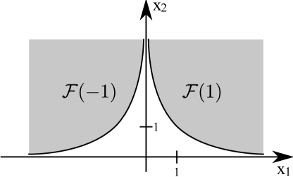
Figure 1: An instance of (Rec) not having any Pareto efficient solution for an uncertainty set $\mathcal{U}$ with only two scenarios.

It is known that all weakly Pareto efficient solutions are optimal solutions of one of the two $\varepsilon$-constraint scalarizations which are given by bounding one of the objective functions while minimizing the other one.

The first scalarization bounds the recovery costs and minimizes the objective function value in the first place, i.e.,

(Rec^class($$\delta {\rm minimize}\ \sup_{\xi\in\mathcal{U}}f(y(\xi),\xi)$$))

s.t. $$d(x,y(\xi))\leq\delta\ \ \mbox{ for all }\xi\in\mathcal{U}$$

$$F(y(\xi),\xi)\leq 0\ \ \mbox{ for all }\xi\in\mathcal{U}$$

$$x\in\mathcal{X},y:\mathcal{U}\to\mathcal{X}.$$

This problem has been introduced as recoverable robustness (see [LLMS09]) and solved in several special cases, e.g., in [KZ15, GDT15, BKK11]. It is hence denoted as the classic scalarization approach.

In our paper we look at the other scalarization in which we minimize the recovery costs while requiring a minimal quality of the recovery solutions:

(Rec($$\varepsilon {\rm minimize}\ \sup_{\xi\in\mathcal{U}}d(x,y(\xi))$$))

s.t. $$f(y(\xi),\xi)\leq\varepsilon\ \ \mbox{ for all }\xi\in\mathcal{U}$$ (2)

$$F(y(\xi),\xi)\leq 0\ \ \mbox{ for all }\xi\in\mathcal{U}$$

$$x\in\mathcal{X},y:\mathcal{U}\to\mathcal{X}$$

Note that Constraints (2) and (3.1) of this second scalarization do not depend on $x$. To determine feasibility of (Rec($\varepsilon$)), we hence check if for every $\xi\in\mathcal{U}$ there exists $y(\xi)$ such that

$$f(y(\xi),\xi)\leq\varepsilon\mbox{ and }F(y(\xi),\xi)\leq 0,$$

i.e., if the sets

$$\mathcal{G}_{\varepsilon}(\xi) := \{y\in\mathcal{X}:F(y,\xi)\leq 0\mbox{ and }f(y,\xi)\leq\varepsilon\}$$

$$= \mathcal{F}(\xi)\cap\{y\in\mathcal{X}:f(y,\xi)\leq\varepsilon\}$$

are not empty for all $\xi\in\mathcal{U}$. To extend some given $x$ to a feasible solution, we choose some $y(\xi)\in\mathcal{G}_{\varepsilon}(\xi)$ which is closest to $x$ w.r.t the metric $d$. This is possible since $\mathcal{G}_{\varepsilon}(\xi)$ is closed: we define

$$d(x,\mathcal{G}_{\varepsilon}(\xi))=\min_{y\in\mathcal{G}_{\varepsilon}(\xi)}d(x,y),$$

where the minimum exists whenever $\mathcal{G}_{\varepsilon}(\xi)\not=\emptyset$.

With $d(x,\emptyset):=\infty$, we can now rewrite (Rec($\varepsilon$)) to an equivalent problem in the (finitely many) $x$-variables only:

(Rec’($$\varepsilon {\rm minimize}\ \sup_{\xi\in\mathcal{U}}d(x,\mathcal{G}_{\varepsilon}(\xi))$$))

$$\mbox{s.t. }x\in\mathcal{X},$$

i.e., $x$ is an optimal solution to (Rec’($\varepsilon$)) if and only if $(x,y)$ with $y(\xi)\in{\rm argmin}_{\mathcal{G}_{\varepsilon}(\xi)}d(x,y)$ is optimal for (Rec($\varepsilon$)).

3.2 Location-based interpretation of (Rec($\varepsilon$))

In a classic location problem (known as the Weber problem or as the Fermat-Torricelli problem, see e.g., [DKSW02]) we have given a set of points, called existing facilities, and we look for a new point minimizing a measure of distance to these given points. If the distance to the farthest point is considered as the objective function, the problem is called center location problem. We have already seen that for given $y:\mathcal{U}\to\mathcal{X}$, our biobjective problem (Rec) reduces to the problem of finding a location $x$ which minimizes the maximum distance to the set $\{y(\xi):\xi\in\mathcal{U}\}$, i.e., a classic center location problem.

We now show that also the $\varepsilon$-constrained version (Rec($\varepsilon$)) of recoverable robustness

$$\min_{x\in\mathcal{X}}\max_{\xi\in\mathcal{U}}d(x,\mathcal{G}_{\varepsilon}(\xi))$$

can be interpreted as the following location problem: The existing facilities are not points but the sets $\mathcal{G}_{\varepsilon}(\xi),\xi\in\mathcal{U}$. (Rec($\varepsilon$)) looks for a new location in the metric space $\mathcal{X}$, namely a point $x\in\mathcal{X}$ which minimizes the maximum distance to the given sets. For a finite uncertainty set $\mathcal{U}$, such location problems have been studied in [BW00, BW02a] for the center objective function and in [BW02b, NPRC03] for median or ordered median objective functions. We adapt the notation of location theory and call such a point (which then is an optimal solution to (Rec($\varepsilon$)) a center with respect to $\{\mathcal{G}_{\varepsilon}(\xi):\xi\in\mathcal{U}\}$ and the distance function $d$. In our further analysis we consider (Rec($\varepsilon$)) from a location’s point of view. To this end, let us denote the objective function of (Rec($\varepsilon$)) by

$$r_{\varepsilon}(x,\mathcal{U})=\sup_{\xi\in\mathcal{U}}d(x,\mathcal{G}_{\varepsilon}(\xi))$$

and let us call $r_{\varepsilon}(x,\mathcal{U})$ the (recovery) radius of $x$ with respect to $\varepsilon$ and $\mathcal{U}$. Let $r_{\varepsilon}^{*}(\mathcal{U})$ denote the best possible recovery radius over $\mathcal{X}$ (if it exists). For a center location $x^{*}$ we then have $r_{\varepsilon}(x^{*},\mathcal{U})=r_{\varepsilon}^{*}(\mathcal{U})$.

The algorithmic advantage drawn from the connection between (Rec($\varepsilon$)) and (point) location problems becomes clear for specific shapes of the sets $\mathcal{G}_{\varepsilon}(\xi).$ For instance, let $P(\xi)$ be given as

$$\min\{\|\xi-x\|:x\in{\rm IR}^{n}\}$$

for some norm $\|\cdot\|$ and $\xi\in\mathcal{U}\subseteq{\rm IR}^{n}$. Then the sets $\mathcal{G}_{\varepsilon}(\xi)$ are scaled and translated unit balls of the norm $\|\cdot\|$, i.e.,

$$\mathcal{G}_{\varepsilon}(\xi)=\{x\in{\rm IR}^{n}:\|x-\xi\|\leq\varepsilon\}.$$

In this case we obtain that

$$d(x,\mathcal{G}_{\varepsilon}(\xi))=\left\{\begin{array}[]{ll}d(x,\xi)-r&\mbox{ if }d(x,\xi)>\varepsilon\\ 0&\mbox{ if }d(x,\xi)\leq\varepsilon\end{array}\right.$$

and it turns out that the center of the location problem with existing (point) facilities $\{\xi:\xi\in\mathcal{U}\}$ is an optimal solution to (Rec($\varepsilon$)) and hence weakly Pareto efficient for (Rec).

3.3 Relation of the biobjective model to other robustness concepts

We first point out the relation between (Rec) and the concept of strict robustness of [BTGN09]. To this end recall from Section 2.2 that ${\rm SR}(\mathcal{U})=\{x\in\mathcal{X}:F(x,\xi)\leq 0\mbox{ for all }\xi\in\mathcal{U}\}$ is the set of strictly robust solutions and RC($\mathcal{U})$ is the strictly robust counterpart of $(P(\xi),\xi\in\mathcal{U})$.

Lemma 1.

Let an uncertain problem $\rm(P(\xi),\xi\in\mathcal{U})$ be given. Then we have:

1. If $\bar{x}$ is an optimal solution to RC($\mathcal{U}$) then $(\bar{x},\bar{y})$ with $\bar{y}(\xi):=\bar{x}\mbox{ for all }\xi\in\mathcal{U}$ is a lexicographically minimal solution to (Rec) w.r.t $({\bf r}(x,y),{\bf f}(y))$.

2. Let $(\bar{x},\bar{y})$ be a lexicographically minimal solution to (Rec) w.r.t $({\bf r}(x,y),{\bf f}(y))$. Then ${\rm SR}(\mathcal{U})\not=\emptyset$ if and only if ${\bf r}(\bar{x},\bar{y})=0$ and in this case $(\bar{x},\bar{y})$ is optimal to RC($\mathcal{U}$).

Proof.

1. Let $\bar{x}$ be an optimal solution to RC($\mathcal{U}$). Define $\bar{y}(\xi):=\bar{x}$ for all $\xi\in\mathcal{U}$. Then ${\bf r}(\bar{x},\bar{y})=0$. Now assume $(\bar{x},\bar{y})$ is not lexicographically minimal. Then there exists $(x^{\prime},y^{\prime})$ with ${\bf r}(x^{\prime},y^{\prime})=0$ and ${\bf f}(y^{\prime})<{\bf f}(\bar{y})$. The first condition yields that $d(x^{\prime},y^{\prime}(\xi))=0$ for all $\xi\in\mathcal{U}$, hence $x^{\prime}=y^{\prime}(\xi)$ for all $\xi\in\mathcal{U}$, and $x^{\prime}\in{\rm SR}(\mathcal{U})$. Using $x^{\prime}=y^{\prime}(\xi)$, the second condition implies $\sup_{\xi\in\mathcal{U}}f(x^{\prime},\xi)<\sup_{\xi\in\mathcal{U}}f(\bar{x},\xi)$, a contradiction to the optimality of $\bar{x}$ for RC($\mathcal{U}$).

2. Now let $(\bar{x},\bar{y})$ be lexicographically minimal to (Rec).

   • Let ${\bf r}(\bar{x},\bar{y})=0$. Then $0={\bf r}(\bar{x},\bar{y})=\sup_{\xi\in\mathcal{U}}d(\bar{x},\bar{y}(\xi))$, i.e., $\bar{x}=\bar{y}(\xi)$ for all $\xi\in\mathcal{U}$. Hence $\bar{x}\in\mathcal{F}(\xi)$ for all $\xi\in\mathcal{U}$, i.e., $\bar{x}\in{\rm SR}(\mathcal{U})$.

   • On the other hand, if ${\rm SR}(\mathcal{U})\not=\emptyset$ there exists $x\in\mathcal{F}(\xi)$ for all $\xi\in\mathcal{U}$. We define $y(\xi):=x$ for all $\xi\in\mathcal{U}$ and obtain ${\bf r}(x,y)=0$. Since $(\bar{x},\bar{y})$ is lexicographically minimal this implies ${\bf r}(\bar{x},\bar{y})=0$.

   Finally, if ${\bf r}(\bar{x},\bar{y})=0$ we already know that $\bar{x}=\bar{y}(\xi)$ for all $\xi\in\mathcal{U}$ and $\bar{x}\in{\rm SR}(\mathcal{U})$, i.e., feasible for RC($\mathcal{U}$). The lexicographic optimality then guarantees that $\bar{x}$ is an optimal solution to RC($\mathcal{U}$).

∎

Sorting the criteria in the objective function in the other order, i.e., minimizing first ${\bf f}(y)$ and then ${\bf r}(x,y)$ is not directly related to any known robustness concept. This lexicographically minimal solution $(x,y)$ realizes an optimal solution $y(\xi)$ in every scenario, and among these optimal solutions minimizes the recovery costs.

Lemma 2.

Let $(x,y)$ be a solution to (Rec) which is lexicographically minimal w.r.t $({\bf f}(y),{\bf r}(x,y))$. Then $f(y(\xi),\xi)=f^{*}(\xi)$ for all $\xi\in\mathcal{U}$.

We now turn our attention to (Rec($\varepsilon$)) and show that this scalarization can be interpreted as adjustable robustness as in [BTGGN04]. Motivated by stochastic programming, the variables in this concept are decomposed into two sets: The values for the here-and-now variables have to be found in the robust optimization algorithm while the decision about the wait-and-see variables can wait until the actual scenario $\xi\in\mathcal{U}$ becomes known. For an uncertain problem $\rm(P(\xi),\xi\in\mathcal{U})$, recall that (Rec($\varepsilon$)) is given as

$$\min_{x\in\mathcal{X}}\sup_{\xi\in\mathcal{U}}d(x,\mathcal{G}_{\varepsilon}(\xi)).$$

We can rewrite this problem in the following way:

$$\min_{z,x}\left\{z:\forall\xi\in\mathcal{U}\ \exists y\in\mathcal{G}_{\varepsilon}(\xi):d(x,y)\leq z\right\}$$

which has the same structure as an adjustable robust problem. As an example, for a problem with linear objective function $f(x,\xi)=c(\xi)^{t}x$, linear constraints $F(x,\xi)=A(\xi)x-b(\xi)\leq 0$, and $\|\cdot\|_{1}$ as recovery norm, we may write

$$\min_{z^{\prime},x}\left\{\sum_{i=1}^{n}z^{\prime}_{i}:\forall\xi\in\mathcal{U}\ \exists y:c(\xi)^{t}y\leq\varepsilon,\ A(\xi)y\leq b(\xi),\ -z^{\prime}\leq x-y\leq z^{\prime}\right\}.$$ (5)

Note that this is a problem without fixed recourse, such that most of the results in [BTGGN04] are not applicable. However, we are still able to apply their results on using heuristic, affinely adjustable counterparts, and Theorem 2.1 from [BTGGN04]:

Theorem 1.

Let $\rm(P(\xi),\xi\in\mathcal{U})$ be an uncertain linear optimization problem, and let the uncertainty be constraint-wise. Furthermore, let there be a compact set $C$ such that $\mathcal{F}(\xi)\subseteq C$ for all $\xi\in\mathcal{U}$. Then, (Rec($\varepsilon$)) is equivalent to the following problem

$$\min_{z,x}\left\{\sum_{i=1}^{n}z^{\prime}_{i}:\exists y\ \forall\xi\in\mathcal{U}:c(\xi)^{t}y\leq\varepsilon,\ A(\xi)y\leq b(\xi),\ -z^{\prime}\leq x-y\leq z^{\prime}\right\}.$$ (6)

Note that problem (6) is a strictly robust problem, which is considerably easier to solve than problem (5). Furthermore, [BTGGN04] show that there is a semidefinite program for ellipsoidal uncertainty sets which is equivalent to problem (5).

Problem (Rec($\varepsilon$)) can also be interpreted as a strictly robust problem in $x$ (see (3.1)). However, the function $\xi\mapsto d(x,\mathcal{G}_{\varepsilon})$ has in general not much properties such that most of the known results cannot be directly applied. Nevertheless, our geometric interpretation gives rise to the results of the next section, in particular within the biobjective setting.

4 Solving (Rec($\varepsilon$))

In this section we investigate the new scalarization (Rec($\varepsilon$)). After a more general analysis of this optimization problem in Section 4.1, we turn our attention to the case of a finite uncertainty set in Section 4.2 where we consider problems with convex and with linear constraints.

4.1 Analysis of (Rec($\varepsilon$))

Let us now describe some general properties of problem (Rec($\varepsilon$)). Since $d$ is a metric we know that

$$0\leq r_{\varepsilon}(x,\mathcal{U})\leq+\infty\ \mbox{ for all }x\in{\rm IR}^{n},$$ (7)

hence the optimal value of (Rec($\varepsilon$)) is bounded by zero from below, although it is $+\infty$ if all points $x$ have infinite radius $r_{\varepsilon}(x,\mathcal{U}).$ This event may happen even when all sets $\mathcal{G}_{\varepsilon}(\xi)$ are non-empty. Indeed, consider, for instance, $\mathcal{X}={\rm IR},$ $\mathcal{G}_{\varepsilon}(\xi)=\{\xi\}$ for all $\xi\in\mathcal{U}={\rm IR}.$ One has, however, that finiteness of $r_{\varepsilon}(x,\mathcal{U})$ at one point $x_{0}$ and one $\varepsilon$ implies finiteness of $r_{\varepsilon^{\prime}}(x,\mathcal{U})$ for all $x\in\mathcal{X}$ and for all $\varepsilon^{\prime}\geq\varepsilon$. In that case we obtain Lipschitz-continuity of the radius, as shown in the following result.

Lemma 3.

Let an uncertain optimization problem $\rm(P(\xi),\xi\in\mathcal{U})$ be given. Suppose there exists $x_{0}\in{\rm IR}^{n}$ such that $r_{\varepsilon}(x_{0},\mathcal{U})<+\infty.$ Then, $r_{\varepsilon}(x,\mathcal{U})<+\infty$ for all $x\in{\rm IR}^{n}$ and for all $\varepsilon^{\prime}\geq\varepsilon$. In such a case, the function ${\rm IR}^{n}\ni x\,\longmapsto r_{\varepsilon^{\prime}}(x,\mathcal{U})$ is Lipschitz-continuous with Lipschitz constant $L=1$ for every $\varepsilon^{\prime}\geq\varepsilon$.

Proof.

Take $x\in{\rm IR}^{n}$ and $\xi\in\mathcal{U}.$ Let $y\in\mathcal{G}_{\varepsilon}(\xi)$ such that $d(x_{0},\mathcal{G}_{\varepsilon}(\xi))=d(x_{0},y).$ We have that

$$d(x,\mathcal{G}_{\varepsilon}(\xi))\leq d(x,y)\leq d(x,x_{0})+d(x_{0},y)=d(x,x_{0})+d(x_{0},\mathcal{G}_{\varepsilon}(\xi))$$

Hence,

$$\max_{\xi\in\mathcal{U}}d(x,\mathcal{G}_{\varepsilon}(\xi))\leq d(x,x_{0})+\max_{\xi\in\mathcal{U}}d(x_{0},\mathcal{G}_{\varepsilon}(\xi))<+\infty,$$

and therefore, $r_{\varepsilon}(x,\mathcal{U})$ is finite everywhere. Since $r_{\varepsilon^{\prime}}(x,\mathcal{U})\leq r_{\varepsilon}(c,\mathcal{U})$ for all $\varepsilon^{\prime}\geq\varepsilon$ we also have finiteness if we increase $\varepsilon$.

We now show that $r_{\varepsilon}(\cdot,\mathcal{U})$ is also Lipschitz-continuous. Let $\delta>0$, and let $x,x^{\prime}\in{\rm IR}^{n}.$ Take $\xi^{*}$ such that

$$\delta+d(x,\mathcal{G}_{\varepsilon}(\xi^{*}))\geq r_{\varepsilon}(x,\mathcal{U}).$$

Since $\mathcal{G}_{\varepsilon}(\xi^{*})$ is closed, take also $y^{\prime}\in\mathcal{G}_{\varepsilon}(\xi^{*})$ such that $d(x^{\prime},\mathcal{G}_{\varepsilon}(\xi^{*}))=d(x^{\prime},y^{\prime}).$

Then,

$$r_{\varepsilon}(x,\mathcal{U})-r_{\varepsilon}(x^{\prime},\mathcal{U}) \leq \delta+d(x,\mathcal{G}_{\varepsilon}(\xi^{*}))-d(x^{\prime},\mathcal{G}_{\varepsilon}(\xi^{*}))$$

$$\leq \delta+d(x,y^{\prime})-d(x^{\prime},y^{\prime})$$

$$\leq \delta+d(x,x^{\prime}).$$

Since this inequality holds for any $\delta>0,$ we obtain $r_{\varepsilon}(x,\mathcal{U})-r_{\varepsilon}(x^{\prime},\mathcal{U})\leq d(x,x^{\prime})$, hence the function $r(\cdot,\mathcal{U})$ is Lipschitz-continuous with Lipschitz constant 1. ∎

In what follows we assume finiteness of the optimal value of (Rec($\varepsilon$)), and thus Lipschitz-continuity of $r_{\varepsilon}(\cdot,\mathcal{U}).$ Hence, (Rec($\varepsilon$)) may be solved by using standard Lipschitz optimization methods [SK10].

For a given $x\in{\rm IR}^{n}$ let us call $\xi\in\mathcal{U}$ a worst-case scenario with respect to $x$ (and $\mathcal{U}$) if

$$d(x,\mathcal{G}_{\varepsilon}(\xi))=r_{\varepsilon}(x,\mathcal{U})$$

and let $WC_{\varepsilon}(x,\mathcal{U})$ be the set of all worst-case scenarios, i.e., scenarios $\xi\in\mathcal{U}$ yielding the maximal recovery distance for the solution $x$. Under certain assumptions, any optimal solution $x^{*}$ to (Rec($\varepsilon$)) has a set $WC_{\varepsilon}(x^{*},\mathcal{U})$ with at least two elements, as shown in the following result.

Lemma 4.

Let an uncertain optimization problem $\rm(P(\xi),\xi\in\mathcal{U})$ be given. Suppose that $\mathcal{U}$ is finite (with at least two elements) and $\mathcal{X}={\rm IR}^{n}$. Fix some $\varepsilon$ and assume that (Rec($\varepsilon$)) attains its optimum at some $x^{*}\in{\rm IR}^{n}.$ Then, $|WC_{\varepsilon}(x^{*},\mathcal{U})|\geq 2$.

Proof.

Finiteness of $\mathcal{U}$ implies that the maximum of $d(x^{*},\mathcal{G}_{\varepsilon}(\xi))$ must be attained at some $\xi.$ Hence, $|WC_{\varepsilon}(x^{*},\mathcal{U})|\geq 1$.

In the case that $r_{\varepsilon}(x^{*},\mathcal{U})=0$, we have that $WC_{\varepsilon}(x^{*},\mathcal{U})=\mathcal{U}$. Thus, let $r_{\varepsilon}(x^{*},\mathcal{U})>0$.

In the case that $WC_{\varepsilon}(x^{*},\mathcal{U})=\{\xi^{*}\}$ for only one scenario $\xi^{*}\in\mathcal{U},$ we can construct a contradiction by finding a different $x$ with a better radius: Take $y^{*}\in\mathcal{G}_{\varepsilon}(\xi^{*})$ such that $d(x^{*},y^{*})=d(x^{*},\mathcal{G}_{\varepsilon}(\xi^{*})),$ and, for $\lambda\in[0,1],$ define $x_{\lambda}$ as

$$x_{\lambda}=(1-\lambda)x^{*}+\lambda y^{*}.$$

Since, by assumption, $WC_{\varepsilon}(x^{*},\mathcal{U})=\{\xi^{*}\}$ and $\mathcal{U}$ is finite, there exists $\delta>0$ such that

$$d(x^{*},\mathcal{G}_{\varepsilon}(\xi))<d(x^{*},\mathcal{G}_{\varepsilon}(\xi^{*}))-\delta\qquad\forall\xi\in\mathcal{U},\,\xi\neq\xi^{*}.$$

Let us show that, for $\lambda$ close to zero, $x_{\lambda}$ has a strictly better objective value than $x^{*},$ which would be a contradiction. First we have

$$d(x_{\lambda},\mathcal{G}_{\varepsilon}(\xi^{*})) \leq d(x_{\lambda},y^{*})$$

$$= (1-\lambda)\|x^{*}-y^{*}\|=(1-\lambda)d(x^{*},\mathcal{G}_{\varepsilon}(\xi^{*}))$$

$$< d(x^{*},\mathcal{G}_{\varepsilon}(\xi^{*}))\text{ for }\lambda>0.$$

For the remaining scenarios $\xi\neq\xi^{*},$

$$d(x_{\lambda},\mathcal{G}_{\varepsilon}(\xi)) \leq \inf_{y\in\mathcal{G}_{\varepsilon}(\xi)}\big{\{}\|x_{\lambda}-x^{*}\|+\|x^{*}-y\|\big{\}}$$

$$= \inf_{y\in\mathcal{G}_{\varepsilon}(\xi)}\big{\{}\lambda\|x^{*}-y^{*}\|+\|x^{*}-y\|\big{\}}$$

$$= \lambda\|x^{*}-y^{*}\|+d(x^{*},\mathcal{G}_{\varepsilon}(\xi))$$

$$< \lambda\|x^{*}-y^{*}\|+d(x^{*},\mathcal{G}_{\varepsilon}(\xi^{*}))-\delta$$

$$< d(x^{*},\mathcal{G}_{\varepsilon}(\xi^{*}))\text{ for }\lambda<\frac{\delta}{\|x^{*}-y^{*}\|}.$$

Hence, for $0<\lambda<\frac{\delta}{\|x^{*}-y^{*}\|}$, we would have that

$$\max_{\xi\in\mathcal{U}}d(x_{\lambda},\mathcal{G}_{\varepsilon}(\xi))<d(x^{*},\mathcal{G}_{\varepsilon}(\xi^{*}))=\max_{\xi\in\mathcal{U}}d(x^{*},\mathcal{G}_{\varepsilon}(\xi)),$$

contradicting the optimality of $x^{*}.$ ∎

If the finiteness assumption of Lemma 4 is dropped, not much can be said about the cardinality of $WC_{\varepsilon}(x,\mathcal{U}),$ since this set can be empty or a singleton:

Example 3.

Let $\mathcal{U}=\{-1,1\}\times[1,\infty),$ and let $F(x,(\xi_{1},\xi_{2}))=(x-\xi_{1})(\xi_{2}x-\xi_{1}\xi_{2}+\xi_{1})$. Let $f(x)=const$ and choose $\varepsilon>const$. It is easily seen that

$$\begin{array}[]{rcl}\mathcal{G}_{\varepsilon}(-1,\xi_{2})=\mathcal{F}(-1,\xi_{2})&=&[-1,-1+\frac{1}{\xi_{2}}]\\ \mathcal{G}_{\varepsilon}(1,\xi_{2})=\mathcal{F}(1,\xi_{2})&=&[1-\frac{1}{\xi_{2}},1]\end{array}$$ (8)

For $x=0,$ $r_{\varepsilon}(x,\mathcal{U})=1,$ but there is no $\xi\in\mathcal{U}$ with $d(x,\mathcal{G}_{\varepsilon}(\xi))=1$. In other words, $WC_{\varepsilon}(0,\mathcal{U})=\emptyset.$

4.2 Solving (Rec($\varepsilon$)) for a finite uncertainty set $\mathcal{U}$

In this section we assume that $\mathcal{U}$ is finite, $\mathcal{U}=\{\xi^{1},\ldots,\xi^{N}\}.$ This simplifies the analysis, since we can explicitly search for a solution $y^{k}=y(\xi^{k})$ for every scenario $\xi^{k}\in\mathcal{U}$. Using the $y^{k}$ as variables we may formulate (Rec($\varepsilon$)) as

$$\begin{array}[]{llll}\min&r\\ \mbox{s.t. }&F(y^{k},\xi^{k})&\leq&0\mbox{ for all }k=1,\ldots,N\\ &f(y^{k},\xi^{k})&\leq&\varepsilon\mbox{ for all }k=1,\ldots,N\\ &d(x,y^{k})&\leq&r\mbox{ for all }k=1,\ldots,N\\ &x\in\mathcal{X},r\in{\rm IR}\\ &y^{k}\in\mathcal{X}&&\phantom{r}\mbox{ for all }k=1,\ldots,N.\end{array}$$ (9)

We can write (Rec($\varepsilon$)) equivalently as

$$\min_{x\in\mathcal{X}}\max_{1\leq k\leq N}d(x,\mathcal{G}_{\varepsilon}(\xi^{k})).$$

Assuming that the distance used is the Euclidean $d_{2}(\cdot,\cdot)$, the function $x\,\longmapsto\max_{k}d_{2}(x,\mathcal{G}_{\varepsilon}(\xi^{k}))$ is known to be d.c. for closed sets $\mathcal{G}_{\varepsilon}$ [HT99], i.e., it can be written as a difference of two convex functions, and then the powerful tools of d.c. programming may be used to find a globally optimal solution if (Rec($\varepsilon$)) is low-dimensional [BCH09], or to design heuristics for more general cases [AT05].

4.2.1 Convex programming problems

We start with optimization problems $\rm P(\xi)$ that have convex sets $\mathcal{G}_{\varepsilon}(\xi)$ for all $\xi\in\mathcal{U}$. This is the case if the functions $F$ and $f$ of $\rm P(\xi)$ are quasiconvex for all fixed scenarios $\xi$, and $\mathcal{X}$ is convex. We furthermore assume that $d$ is convex, which is the case, e.g., when $d$ has been derived from a norm, i.e. $d(x,y)=\|y-x\|$ for some norm $\|\cdot\|$.

Let us fix $\xi$. Then the function ${\rm IR}^{n}\ni x\longmapsto d(x,\mathcal{F}(\xi))$ describes the distance between a point and a convex set and is hence convex. We conclude that also $r_{\varepsilon}(x,\mathcal{U})$ is convex, being the maximum of a finite set of convex functions.

Lemma 5.

Consider an uncertain optimization problem $\rm(P(\xi),\xi\in\mathcal{U})$ with quasiconvex objective function $f(\cdot,\xi)$ and quasiconvex constraints $F(\cdot,\xi)$ for any fixed $\xi$. Let $\mathcal{X}\subseteq{\rm IR}^{n}$ be convex, $\mathcal{U}$ be a finite set and $d$ be convex. Then problem (Rec($\varepsilon$)) is a convex optimization problem.

In order to solve (Rec($\varepsilon$)) one can hence apply algorithms suitable for convex programming, e.g., subgradient or bundle methods [SY06, HUL93]. In particular, if (Rec($\varepsilon$)) is unconstrained in $x$, a necessary and sufficient condition for a point $x^{*}$ to be an optimal solution is

$$0\in\partial(r_{\varepsilon}(x^{*},\mathcal{U})),$$

i.e., if $0$ is contained in the subdifferential of $r_{\varepsilon}(\cdot,\mathcal{U})$ at the point $x^{*}$. By construction of $r_{\varepsilon}(\cdot,\mathcal{U}),$ we obtain

$$0\in{\rm conv}\left\{\partial d(x^{*},\mathcal{G}_{\varepsilon}(\xi)):\xi\in WC_{\varepsilon}(x^{*},\mathcal{U})\right\}$$

where $WC_{\varepsilon}(x^{*},\mathcal{U})$ is the set of worst-case scenarios (see [HUL93]), and $\partial d(x^{*},\mathcal{G}_{\varepsilon}(\xi))$ is the subdifferential of $d(\cdot,\mathcal{G}_{\varepsilon}(\xi))$ at $x^{*}$.

Now, $\partial d(x^{*},\mathcal{G}_{\varepsilon}(\xi))$ can be written in terms of the subdifferential of the distance used, see [CF02], where also easy representations for polyhedral norms or the Euclidean norm are presented. Although we do not know much a priori about the number of worst-case scenarios, we do not need to investigate all possible subsets but may restrict our search to sets which do not have more than $n+1$ elements as is shown in our next result. This may be helpful in problems with a large number of scenarios but low dimension $n$ for the decisions.

Theorem 2.

Let $\mathcal{U}$ be finite with cardinality of at least $n+1$. Let $\mathcal{X}={\rm IR}^{n}$. Suppose (Rec($\varepsilon$)) attains its optimum at some $x^{*}$, and that for each $\xi$ the functions $F(\cdot,\xi)$ and $f(\cdot,\xi)$ are quasiconvex. Let $d$ be convex. Then there exists a subset $\overline{\mathcal{U}}\subseteq\mathcal{U}$ of scenarios with $2\leq|\overline{\mathcal{U}}|\leq n+1$ such that

$$r_{\varepsilon}^{*}(\mathcal{U})=r_{\varepsilon}(x^{*},\mathcal{U})=r_{\varepsilon}(x^{*},\overline{\mathcal{U}})=r_{\varepsilon}^{*}(\overline{\mathcal{U}}).$$

Proof.

Let $x^{*}$ be optimal for (Rec($\varepsilon$)). The result is trivial if $r_{\varepsilon}(x^{*},\mathcal{U})=0$: take any collection of $n+1$ scenarios. Hence, we may assume $r_{\varepsilon}(x^{*},\mathcal{U})>0,$ which implies that $x^{*}$ does not belong to all sets $\mathcal{G}_{\varepsilon}(\xi).$

By Lemma 4, $|WC_{\varepsilon}(x^{*},\mathcal{U})|\geq 2$. If $|WC_{\varepsilon}(x^{*},\mathcal{U})|\leq n+1,$ then we are done. Otherwise, $|WC_{\varepsilon}(x^{*},\mathcal{U})|>n+1,$ we have by the optimality of $x^{*}$ and convexity of the functions $d(\cdot,\mathcal{G}_{\varepsilon}(\xi)),$ that

$$0\in{\rm conv}\left\{\partial d(x^{*},\mathcal{G}_{\varepsilon}(\xi)):\xi\in WC_{\varepsilon}(x^{*},\mathcal{U})\right\}$$

By Carathéodory’s theorem, $WC_{\varepsilon}(x^{*},\mathcal{U})$ contains a subset $\overline{\mathcal{U}},$ $1\leq|\overline{\mathcal{U}}|\leq n+1$ such that $0\in{\rm conv}\left\{\partial d(x^{*},\mathcal{G}_{\varepsilon}(\xi)):\xi\in\overline{\mathcal{U}}\right\}.$ Such $\overline{\mathcal{U}}$ clearly satisfies the conditions stated. ∎

4.2.2 Problems with linear constraints and polyhedral norms as recovery costs

As in the section before, we assume a finite uncertainty set $\mathcal{U}=\{\xi^{1},\ldots,\xi^{N}\}$. Let us now consider the case that all sets $\mathcal{G}_{\varepsilon}(\xi^{k})$, $k=1,\ldots,N$ are polyhedral sets. More precisely, we consider problems of type

$$\mbox{P($\xi$)}\hskip 28.45274pt\min\ f(x,\xi):=c(\xi)^{t}x$$

s.t. $$F(x,\xi):=A(\xi)x-b(\xi)\leq 0$$

$$x\in\mathcal{X}$$

with a finite uncertainty set $\mathcal{U}=\{\xi^{1},\ldots,\xi^{N}\}$, linear constraints $A(\xi)x\leq b(\xi)$ for every $\xi\in\mathcal{U}$, a linear objective function $c(\xi)^{t}x$ and a polyhedron $\mathcal{X}.$

Furthermore, let us assume that the distance $d$ is induced by a block norm $\|\cdot\|$, i.e., a norm whose unit ball is a polytope, see [WWR85, Wit64]. The most prominent examples for block norms are the Manhattan ($d_{1}$) and the maximum ($d_{\infty}$) norm, which both may be suitable to represent recovery costs: In the case that the recovery costs are obtained by adding single costs of each component, the Manhattan norm is the right choice. The maximum norm may represent the recovery time in the case that a facility has to be moved along each coordinate (or a schedule has to be updated by a separate worker in every component) and the longest time determines the time for the complete update.

We also remark that it is possible to approximate any given norm arbitrarily close by block norms, since the class of block norms is a dense subset of all norms, see [WWR85]. Thus, the restriction to the class of block norms may not be a real restriction in a practical setting.

The goal of this section is to show that under the assumptions above, (Rec($\varepsilon$)) is a linear program.

We start with some notation. Given a norm $\|\cdot\|$, let

$$B=\{x\in{\rm IR}^{n}:\|x\|\leq 1\}$$

denote its unit ball. Recall that the unit ball of a block norm $\|\cdot\|$ is a full-dimensional convex polytope which is symmetric with respect to the origin. Since such a polytope has a finite number $S$ of extreme points, we may denote in the following the extreme points of $B$ as

$$\mathrm{Ext}(B)=\{e_{i}:1\leq i\leq S\}.$$

Since $B$ is symmetric with respect to the origin, $S\in{\rm IN}$ is always an even number and for any $e_{i}\in\mathrm{Ext}(B)$ there exists another $e_{j}\in\mathrm{Ext}(B)$ such that $e_{i}=-e_{j}$. Its dual (or polar) norm defined as $\|x\|_{0}:=\max\{x^{t}y:\|y\|\leq 1\}$ has the unit ball

$$B^{0}=\{x\in{\rm IR}^{n}:x^{t}y\leq 1\mbox{ for all }y\in B\}.$$

It is known that $B^{0}$ is again a polyhedral norm with extreme points

$$\mathrm{Ext}(B^{0})=\{e^{0}_{i}:1\leq i\leq S^{0}\},$$

where $S^{0}$ is the number of facets of $B$ (see, e.g., [Roc70]).

The following property is crucial for the linear programming formulation of (Rec($\varepsilon$)). It shows that it is sufficient to consider only the extreme points $\mathrm{Ext}(B)$ of either the unit ball $B$ of the block norm, or of the unit ball $B^{0}$ of its polar norm in order to compute $\|x\|$ for any point $x\in{\rm IR}^{n}$.

Lemma 6 ([WWR85]).

Let $\mathrm{Ext}(B)=\{e_{i}:1\leq i\leq S\}$ be the extreme points of a block norm $\|\cdot\|$ with unit ball $B$ and let $\mathrm{Ext}(B^{0})=\{e^{0}_{i}:1\leq i\leq S^{0}\}$ be the extreme points of its polar norm with unit ball $B^{0}$. Then $\|\cdot\|$ has the following two characterizations:

$$\|x\|=\min\left\{\sum_{i=1}^{S}\beta_{i}:x=\sum_{i=1}^{S}\beta_{i}e_{i},~{}\beta_{i}\geq 0\>\forall\>i=1,\ldots,S\right\}$$

and

$$\|x\|=\max_{i=1,\ldots,S^{0}}x^{t}e_{i}^{0}.$$

Lemma 6 implies that we can compute $\|x-y\|$ for any pair $x,y\in{\rm IR}^{n}$ by linear programming. Thus, our assumptions on the sets $\mathcal{G}_{\varepsilon}(\xi^{k})$ and Lemma 6 give rise to the following linear formulations of (Rec($\varepsilon$)), if $\mathcal{X}$ is a polyhedron:

$$\min\quad r$$

s.t. $$A(\xi^{k})y^{k} \quad\leq\quad b(\xi^{k}) \mbox{ for all }k=1,\ldots,N$$ (10)

$$c(\xi^{k})^{t}y^{k} \quad\leq\quad \varepsilon \mbox{ for all }k=1,\ldots,N$$ (11)

$$y^{k}-x \quad=\quad \sum_{i=1}^{S}\beta^{k}_{i}e_{i} \mbox{ for all }k=1,\ldots,N$$ (12)

$$\sum_{i=1}^{S}\beta^{k}_{i} \quad\leq\quad r \mbox{ for all }k=1,\ldots,N$$ (13)

$$x,y^{k} \quad\in\quad \mathcal{X} \mbox{ for all }k=1,\ldots,N$$ (14)

$$r,\beta^{k}_{i} \quad\geq\quad 0 \mbox{ for all }k=1,\ldots,N,\ i=1,\ldots,S$$ (15)

Note that constraints (10) and (11) are just the definition of the sets $\mathcal{G}_{\varepsilon}(\xi^{k})$. Furthermore, (12) and (13) together ensure that $\|x-y^{k}\|\leq r$ for all $k=1,\ldots,N$. Hence, the linear program is equivalent to the formulation (9) for a finite set of scenarios each of them having a polyhedron as feasible set and if a block norm is used as distance measure. In this case we have hence shown that (Rec($\varepsilon$)) can be formulated as a linear program. In order to use the second characterization of block norms in Lemma 6 we replace (12) and (13) by

$$\left(e_{i}^{0}\right)^{t}(y^{k}-x)\leq r\quad\mbox{ for all }k=1,\ldots,N,\ i=1,\ldots,S^{0}$$ (16)

to ensure that the value of $\|x-y^{k}\|$ is correctly computed. We summarize our findings in the following result.

Theorem 3.

Consider an uncertain linear optimization problem $\rm(P(\xi),\xi\in\mathcal{U})$ Let $\mathcal{U}=\{\xi^{k}:k=1,\ldots,N\}$ be a finite set and let $d$ be induced by a block norm. Let $\mathcal{X}\subseteq{\rm IR}^{n}$ be a polyhedron. Then (Rec($\varepsilon$)) can be solved by linear programming.

If the number of constraints defining $\mathcal{X}$, and either the number of extreme points of $B$ or the number of facets of $B$ depend at most polynomially on the dimension $n$, then (Rec($\varepsilon$)) can be solved in polynomial time.

We note that block norms may be generalized to the broader class of polyhedral gauges where the symmetry assumption on the unit ball is dropped (see e.g., [NP09]). Nevertheless it is readily shown that Lemma 6 applies to polyhedral gauges as well. Hence, it follows that Theorem 3 also holds for distance functions derived from polyhedral gauges.

4.2.3 Problems with hyperplanes as feasible sets

We consider a special case in which (Rec($\varepsilon$)) can be rewritten as a linear program, even though the distance measure does not need to be derived from a block norm, namely if the sets $\mathcal{G}_{\varepsilon}(\xi)$ are all hyperplanes or halfspaces. Before we show the resulting linear program for this case, we consider some situations in which this happens:

Example 4.

Let $d$ be a distance derived from a norm, and let $\mathcal{X}={\rm IR}^{n}$.

1. For feasibility problems of type

   $$\mbox{P$(a,b)$}\hskip 28.45274pt\min\ const$$

   s.t. $$F(x,(a,b)):=a^{t}x-b=0$$

   with $\mathcal{U}=\{(a^{1},b^{1}),\ldots,(a^{N},b^{N})\}$, $a^{1},\ldots,a^{N}\neq 0$ we obtain $\mathcal{G}_{\varepsilon}(a^{k},b^{k})=\{x:{a^{k}}^{t}x-b^{k}=0\}$ for all $\varepsilon>const$.

2. The same holds for problems

   $$P(\xi)\ \ \min\{f(x,\xi):x\in\mathcal{F}(\xi)\}\mbox{ for }\xi\in\mathcal{U}$$

   if $\mathcal{F}(\xi)$ is a hyperplane for each $\xi\in\mathcal{U}$ and $\varepsilon>f(x,\xi)$ for all $x\in\mathcal{F}(\xi)$.

3. For unconstrained uncertain linear optimization of the form

   $$P(\xi)\ \ \min\{c(\xi)^{t}x:x\in{\rm IR}^{n}\}$$

   the resulting sets $\mathcal{G}_{\varepsilon}(\xi^{k})=\{x:c(\xi)^{t}x\leq\varepsilon\}$ are halfspaces.

Let us first consider the case of hyperplanes: For $\xi^{k}=(a^{k},b^{k})$, let $\mathcal{G}_{\varepsilon}(\xi)=H_{a^{k},b^{k}}=\{x\in{\rm IR}^{n}:{a^{k}}^{t}x=b^{k}\}$ be a hyperplane. Then (Rec($\varepsilon$)) is given by

$$\min\ r$$

s.t. $$d(x,H_{a^{k},b^{k}})\leq r\mbox{ for all }k=1,\ldots,N$$

$$x\in{\rm IR}^{n},r\in{\rm IR},$$

Recall the point-to-hyperplane distance [PC01]

$$d(x,H_{a,b})=\frac{|a^{t}x-b|}{\|a\|^{\circ}},$$

where $\|\cdot\|^{\circ}$ denotes the dual norm to $\|\cdot\|$. As the values of $\|a^{k}\|^{\circ}$ can be precomputed and the absolute value linearized, we gain a linear program

$$\min\ r$$

s.t. $$-r\leq\frac{{a^{k}}^{t}x-b}{\|a^{k}\|^{\circ}}\leq r\mbox{ for all }k=1,\ldots,N$$ (17)

$$x\in{\rm IR}^{n},r\in{\rm IR}.$$

For halfspaces $\mathcal{G}_{\varepsilon}(\xi^{k})=H^{+}_{a^{k},b^{k}}=\{x\in{\rm IR}^{n}:{a^{k}}^{t}x\leq b^{k}\}$ instead of hyperplanes, the distance is given by

$$d(x,H^{+}_{a,b})=\frac{|a^{t}x-b|^{+}}{\|a\|^{\circ}},$$

where $|a^{t}x-b|^{+}=\max\{a^{t}x-b,0\}$, resulting in the linear program

$$\min\ r$$

s.t. $$\frac{{a^{k}}^{t}x-b}{\|a^{k}\|^{\circ}}\leq r\mbox{ for all }k=1,\ldots,N$$ (18)

$$r\geq 0$$

$$x\in{\rm IR}^{n},r\in{\rm IR}.$$

Theorem 4.

Consider an uncertain optimization problem with finite uncertainty set and sets $\mathcal{G}_{\varepsilon}(\xi)$ that are hyperplanes or halfspaces. Let $\mathcal{X}={\rm IR}^{n}$ and let $d$ be derived from a norm $\|\cdot\|$. Then (Rec($\varepsilon$)) can be formulated as linear program (see (17) and (18)) and be solved in polynomial time, provided that the dual norm of $\|\cdot\|$ can be evaluated in polynomial time.

5 Reduction approaches

In this section we analyze recoverable-robust solutions for different uncertainty sets $\mathcal{U}$, and hence write Rec($\mathcal{U}$), ${\bf f_{\mathcal{U}}}$ and ${\bf r_{\mathcal{U}}}$ to emphasize the uncertainty set that is considered:

Rec($$\mathcal{U} {\rm minimize}\ \left({\bf f_{\mathcal{U}}}(y),{\bf r_{\mathcal{U}}}(x,y)\right)=\left(\sup_{\xi\in\mathcal{U}}f(y(\xi),\xi),\sup_{\xi\in\mathcal{U}}d(x,y(\xi))\right)$$)

$$\mbox{s.t. }F(y(\xi),\xi)\leq 0\ \ \mbox{ for all }\xi\in\mathcal{U}$$

$$x\in\mathcal{X},y:\mathcal{U}\to\mathcal{X}$$

Recall that a solution $x$ is recoverable-robust with respect to $\mathcal{U}$ if there exists $y:\mathcal{U}\to\mathcal{X}$ such that $(x,y)$ is Pareto-efficient for Rec($\mathcal{U}$).

The main goal of this section is to reduce the set $\mathcal{U}$ to a smaller (maybe even finite) set $\mathcal{U}^{\prime}\subseteq\mathcal{U}$, such that the set of recovery-robust solutions does not change. This is the case if we can extend any feasible solution $(x,y^{\prime})$ for Rec($\mathcal{U}^{\prime}$) to a feasible solution $(x,y)$ for Rec($\mathcal{U}$) without changing the objective function values.

Lemma 7.

Let $\mathcal{U}^{\prime}\subseteq\mathcal{U}$. If for all feasible solutions $(x,y^{\prime})$ of Rec($\mathcal{U}^{\prime}$) there exists $y:\mathcal{U}\to\mathcal{X}$ such that

• $(x,y)$ is feasible for Rec($\mathcal{U}$), i.e., $F(y(\xi),\xi)\leq 0$ for all $\xi\in\mathcal{U}$, and

• ${\bf f_{\mathcal{U}}}(y)={\bf f_{\mathcal{U}^{\prime}}}(y^{\prime})$ and ${\bf r_{\mathcal{U}}}(x,y)={\bf r_{\mathcal{U}^{\prime}}}(x,y^{\prime})$

then Rec($\mathcal{U}$) and Rec($\mathcal{U}^{\prime}$) have the same recoverable-robust solutions.

Proof.

Let $(x,y)$ be feasible for Rec($\mathcal{U}$). Define

$$y_{|\mathcal{U}^{\prime}}:\mathcal{U}^{\prime}\to\mathcal{X}\ \mbox{ through }y_{|\mathcal{U}^{\prime}}(\xi):=y(\xi)\ \mbox{ for all }\xi\in\mathcal{U}^{\prime}$$

Then $(x,y^{\prime})$ is feasible for Rec($\mathcal{U}^{\prime}$) and ${\bf f_{\mathcal{U}^{\prime}}}(y^{\prime})\leq{\bf f_{\mathcal{U}}}(y)$, ${\bf r_{\mathcal{U}^{\prime}}}(x,y^{\prime})\leq{\bf r_{\mathcal{U}}}(x,y)$. Together with the assumption of this lemma Pareto optimality follows since a solution can be improved by switching between Rec($\mathcal{U}$) and Rec($\mathcal{U}^{\prime}$):

• Let $x$ be recoverable-robust w.r.t $\mathcal{U}$. Then there exists $y:\mathcal{U}\to\mathcal{X}$ such that $(x,y)$ is Pareto efficient for Rec($\mathcal{U}$). Define $y^{\prime}:=y_{|\mathcal{U}^{\prime}}$. Then $(x,y^{\prime})$ is Pareto-efficient for Rec($\mathcal{U}^{\prime}$): Assume that $(\tilde{x},\tilde{y}^{\prime})$ dominates $(x,y^{\prime})$. Due to the assumption of this lemma there exists $(\tilde{x},\tilde{y})$ which is feasible for Rec($\mathcal{U}$) and ${\bf f_{\mathcal{U}}}(\tilde{y})={\bf f_{\mathcal{U}^{\prime}}}(\tilde{y}^{\prime})$ and ${\bf r_{\mathcal{U}}}(\tilde{x},\tilde{y})={\bf r_{\mathcal{U}^{\prime}}}(\tilde{x},\tilde{y}^{\prime})$, i.e., $(\tilde{x},\tilde{y})$ then dominates $(x,y)$, a contradiction.

• Let $x$ be recoverable-robust w.r.t $\mathcal{U}^{\prime}$. Then there exists $y^{\prime}:\mathcal{U}^{\prime}\to\mathcal{X}$ such that $(x,y^{\prime})$ is Pareto-efficient for Rec($\mathcal{U}^{\prime}$). Choose $y$ according to the assumption of this lemma. Then $(x,y)$ is Pareto-efficient for Rec($\mathcal{U}$): Assume that $(\tilde{x},\tilde{y})$ dominates $(x,y)$. Then $(\tilde{x},\tilde{y}_{|\mathcal{U}^{\prime}})$ is feasible for Rec($\mathcal{U}^{\prime}$) and ${\bf f_{\mathcal{U}^{\prime}}}(\tilde{y}_{|\mathcal{U}^{\prime}})\leq{\bf f_{\mathcal{U}}}(\tilde{y})$ and ${\bf r_{\mathcal{U}^{\prime}}}(\tilde{x},\tilde{y}_{|\mathcal{U}^{\prime}})\leq{\bf r_{\mathcal{U}}}(\tilde{x},\tilde{y})$, i.e., $(\tilde{x},\tilde{y}_{|\mathcal{U}^{\prime}})$ then dominates $(x,y^{\prime})$, a contradiction.

∎

We now use Lemma 7 to reduce the set of scenarios $\mathcal{U}$. Our first result is similar to the reduction rules for set covering problems [TSRB71].

Lemma 8.

If P($\xi^{2}$) is a relaxation of P($\xi^{1}$) for two scenarios $\xi^{1},\xi^{2}\in\mathcal{U}$, then Rec($\mathcal{U}$) and Rec($\mathcal{U}\setminus\{\xi^{2}\}$) have the same recoverable robust solutions, i.e., scenario $\xi^{2}$ may be ignored.

Proof.

We check the condition of Lemma 7: Let $(x,y^{\prime})$ be feasible for Rec($\mathcal{U}\setminus\{\xi^{2}\}$). Define

$$y:\mathcal{U}\to\mathcal{X}\ \mbox{ through }y(\xi):=\left\{\begin{array}[]{ll}y^{\prime}(\xi)\mbox{ if }\xi\in\mathcal{U}\setminus\{\xi^{2}\}\\ y^{\prime}(\xi^{1})\mbox{ if }\xi=\xi^{2}\end{array}\right.$$

Then $(x,y)$ is feasible since $F(y(\xi),\xi)\leq 0$ for all $\xi\in\mathcal{U}\setminus\{\xi^{2}\}$ and $F(y(\xi^{2}),\xi^{2})=F(y(\xi^{1}),\xi^{2})\leq 0$ since $F(y(\xi^{1}),\xi^{1})\leq 0$ and P($\xi^{2}$) is a relaxation of P($\xi^{1}$). Furthermore, $f(y(\xi^{2}),\xi^{2})=f(y(\xi^{1}),\xi^{2})\leq f(y(\xi^{1}),\xi^{1})$ implies

$${\bf f_{\mathcal{U}}}(y)=\sup_{\xi\in\mathcal{U}}f(y(\xi),\xi)=\sup_{\xi\in\mathcal{U}\setminus\{\xi^{2}\}}f(y(\xi),\xi)=\sup_{\xi\in\mathcal{U}\setminus\{\xi^{2}\}}f(y^{\prime}(\xi),\xi)={\bf f_{\mathcal{U}\setminus\{\xi^{2}\}}}(y^{\prime}).$$

Finally, $y(\xi^{1})=y(\xi^{2})$, hence

$${\bf r_{\mathcal{U}}}(x,y)=\sup_{\xi\in\mathcal{U}}d(x,y(\xi))=\sup_{\xi\in\mathcal{U}\setminus\{\xi^{2}\}}d(x,y(\xi))=\sup_{\xi\in\mathcal{U}\setminus\{\xi^{2}\}}d(x,y^{\prime}(\xi))={\bf r}_{\mathcal{U}\setminus\{\xi^{2}\}}(x,y^{\prime}).$$

∎

Note that depending on the definition of the optimization problem and the uncertainty set $\mathcal{U}$, often large classes of scenarios may be dropped. This is in particular the case if the sets $\mathcal{F}(\xi)$ are nested.

In the following we are interested in identifying a kind of core set $\mathcal{U}^{\prime}\subseteq\mathcal{U}$ containing a finite number of scenarios which are sufficient to consider in order to solve the recoverable-robust counterpart. More precisely, we look for a finite set $\mathcal{U}^{\prime}$ such that Rec($\mathcal{U})$ and Rec($\mathcal{U}^{\prime})$ have the same recoverable-robust solutions.

In the following we consider a polytope $\mathcal{U}$ with a finite number of extreme points $\xi^{1},\ldots,\xi^{N}$, i.e., let

$$\mathcal{U}=conv(\mathcal{U}^{\prime})\ \mbox{ where }\ \mathcal{U}^{\prime}=\{\xi^{1},\ldots,\xi^{N}\}.$$

Then many robustness concepts have (under mild conditions) the following property: Instead of investigating all $\xi\in\mathcal{U}$, it is enough to investigate the extreme points $\xi^{1},\ldots,\xi^{N}$ of $\mathcal{U}$. For example, for the strictly robust counterpart RC$(\mathcal{U})$ of an uncertain optimization problem ($P(\xi),\xi\in\mathcal{U}=conv\{\xi^{1},\ldots,\xi^{N}\}$), RC$(\mathcal{U})$ is equivalent to RC$(\{\xi^{1},\ldots,\xi^{N}\})$, if $F(x,\cdot)$ is convex for all $x\in\mathcal{X}$.

Unfortunately, a similar result for the recoverable-robust counterpart does not hold. This means that the set of Pareto efficient solutions of Rec($\mathcal{U}^{\prime}$) does in general not coincide with the set of Pareto efficient solutions of Rec($\mathcal{U}$) with respect to the larger set $\mathcal{U}=conv(\mathcal{U}^{\prime})$ as demonstrated in the following example.

Example 5.

Consider the following uncertain optimization problem:

$$\mbox{P($a_{1},a_{2},b$)}\hskip 28.45274pt\min\ f(x_{1},x_{2})=const$$

s.t. $$a_{1}x_{1}+a_{2}x_{2}-b=0$$

$$x_{1},x_{2}\in{\rm IR},$$

where

$$\mathcal{U}=conv(\mathcal{U}^{\prime})\text{ with }\mathcal{U}^{\prime}=\{(1,0,0),(0,1,0),(1,1,2)\}.$$

Let the recovery distance be the Euclidean distance. Then $x^{*}=(2-\sqrt{2},2-\sqrt{2})$, the midpoint of the incircle of the triangle that is given by the intersections of the respective feasible solutions, is a Pareto efficient solution of Rec($\mathcal{U}^{\prime})$, as it is the unique minimizer of the recovery distance (see Figure 2(a)).

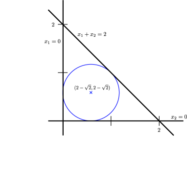
(a) Optimal solution w.r.t. $\mathcal{U}^{\prime}$.

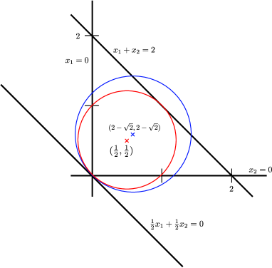
(b) Optimal solution w.r.t. $\mathcal{U}$.

Figure 2: Rec($\mathcal{U}^{\prime})$ and Rec($\mathcal{U})$ may have different optimal solutions.

On the other hand, this solution is not Pareto efficient when the convex hull of $\mathcal{U}^{\prime}$ is taken into consideration. Indeed, by elementary geometry, one finds that

$$r(x^{*},\mathcal{U}) =\sqrt{2}\cdot(2-\sqrt{2})\approx 0.828,$$

$$r(\bar{x},\mathcal{U}) =\frac{1}{\sqrt{2}}\approx 0.707,$$

where $\bar{x}=(\frac{1}{2},\frac{1}{2})$ (see Figure 2(b)). Therefore, solving Rec($\mathcal{U}^{\prime})$ does not give the set of Pareto efficient solutions for Rec($\mathcal{U})$ .

However, assuming more problem structure, we can give the following result.

Theorem 5.

Consider an uncertain optimization problem with uncertainty set $\mathcal{U}=conv(\mathcal{U}^{\prime})$ with $\mathcal{U}^{\prime}:=\{\xi^{1},\ldots,\xi^{N}\}$. Let $F$ consist of $m$ constraints with $F_{i}:{\rm IR}^{n}\times\mathcal{U}\to{\rm IR}$, $i=1,\ldots,m$ and $f:{\rm IR}^{n}\times\mathcal{U}\to{\rm IR}$ be jointly quasiconvex in the arguments $(y,\xi)$. Let $d(x,\cdot)$ be quasiconvex. Let $\mathcal{X}$ be convex.

Then Rec($\mathcal{U}$) and Rec($\mathcal{U}^{\prime}$) have the same set of recoverable-robust solutions.

Proof.

Let $(x,y^{\prime})$ be feasible for Rec($\mathcal{U}^{\prime}$). We first define $y:\mathcal{U}\to\mathcal{X}$.

Let $\xi\in\mathcal{U}$. Then there exist $\lambda_{i},i=1,\ldots,N$ such that $\xi=\sum_{i=1}^{N}\lambda_{i}\xi^{i}$ with $\sum_{i=1}^{N}\lambda_{i}=1$ and $\lambda_{i}\geq 0$. We set $y(\xi):=\sum_{i=1}^{N}\lambda_{i}y^{\prime}(\xi^{i})$. Note that this implies $y(\xi^{i})=y^{\prime}(\xi^{i})$ for all $i=1,\ldots,N$. We now check the conditions of Lemma 7.

For every constraint $k=1,\ldots,m$ the joint quasiconvexity implies that

$$F_{k}(y(\xi),\xi)=F_{k}\left(\sum_{i=1}^{N}\lambda_{i}y(\xi^{i}),\sum_{i=1}^{N}\lambda_{i}\xi^{i}\right)\leq\max_{i=1,\ldots,N}F_{k}(y(\xi^{i}),\xi^{i})\leq 0\ \forall k=1,\ldots,m,$$

where the last inequality holds since $y(\xi^{i})=y^{\prime}(\xi^{i})$ and $(x,y^{\prime})$ is feasible for Rec($\mathcal{U}^{\prime}$). We hence have that $(x,y)$ is feasible for Rec($\mathcal{U}$).

Analogously, joint quasiconvexity of $f$ implies $f(y(\xi),\xi)\leq\max_{i=1,\ldots,N}f(y(\xi^{i}),\xi^{i})$ for all $\xi\in\mathcal{U}$, hence

$${\bf f_{\mathcal{U}}}(y)=\sup_{\xi\in\mathcal{U}}f(y(\xi),\xi)=\max_{\xi\in\mathcal{U}^{\prime}}f(y(\xi),\xi)=\max_{\xi\in\mathcal{U}^{\prime}}f(y^{\prime}(\xi),\xi)={\bf f_{\mathcal{U}^{\prime}}}(y^{\prime}).$$

Finally, for the recovery distance $d$ we assumed quasiconvexity in its second argument which implies $d(x,y(\xi))\leq\max_{i=1,\ldots,N}d(x,y(\xi^{i}))$, hence

$${\bf r_{\mathcal{U}}}(x,y)=\sup_{\xi\in\mathcal{U}}d(x,y(\xi))=\max_{\xi\in\mathcal{U}^{\prime}}d(x,y(\xi))=\max_{\xi\in\mathcal{U}^{\prime}}d(x,y^{\prime}(\xi))={\bf r_{\mathcal{U}^{\prime}}}(x,y^{\prime}).$$

∎

An important particular case of Theorem 5 is the case in which

$$F(x,\xi)=G(x)-b(\xi)$$

for a convex $G$ and concave $b$ (i.e., the uncertainty is in the right-hand side), since $F$ is then jointly quasiconvex in $(x,\xi)$.

Corollary 1.

Let $\rm(P(\xi),\xi\in\mathcal{U})$ be an uncertain optimization problem with uncertainty set $\mathcal{U}=conv(\mathcal{U}^{\prime})$ with $\mathcal{U}^{\prime}:=\{\xi^{1},\ldots,\xi^{N}\}$. Let $F(x,\xi)=G(x)-b(\xi)$ with a convex function $G:{\rm IR}^{n}\to{\rm IR}^{m}$ and a concave function $b(\xi):{\rm IR}^{M}\to{\rm IR}^{m}$. Let $f(x,\xi)$ be jointly quasiconvex, $\mathcal{X}$ be convex, and let $d(x,\cdot)$ be quasiconvex. Then Rec($\mathcal{U})$ and Rec($\mathcal{U}^{\prime})$ have the same recoverable-robust solutions.

We remark that $G$ must not depend on the scenario $\xi$. Example 5 shows that Corollary 1 is not even true for a linear function $F(x,\xi)=A(\xi)x-b(\xi)$: If the matrix $A$ is dependent on $\xi$, we cannot conclude that Rec($\mathcal{U})$ and Rec($\mathcal{U}^{\prime})$ have the same recoverable-robust solutions.

Note that Corollary 1 applies in particular for the special case where $b(\xi)=\xi$, i.e., for uncertain convex optimization problems of the type

$${\rm P}(b)\ \min_{x\in{\rm IR}^{n}}\{f(x):G(x)\leq b\}.$$ (19)

In particular we know for P($b$) that the center with respect to some finite set $\mathcal{U}^{\prime}$ solves the uncertain problem with respect to $\mathcal{U}=conv(\mathcal{U}^{\prime})$.

This means we can use the finite set $\mathcal{U}^{\prime}$ instead of $\mathcal{U}$ when solving (Rec) if the conditions of the previous theorem apply. This is summarized next.

Corollary 2.

Let $\rm(P(\xi),\xi\in\mathcal{U})$ be an uncertain optimization problem with uncertainty set $\mathcal{U}=conv(\mathcal{U}^{\prime})$ with $\mathcal{U}^{\prime}:=\{\xi^{1},\ldots,\xi^{N}\}$ and with constraints $F(x,\xi)=G(x)-b(\xi)$ with a convex function $G:{\rm IR}^{n}\to{\rm IR}^{m}$ and a concave function $b(\xi):{\rm IR}^{M}\to{\rm IR}^{m}$. Let $\mathcal{X}\subseteq{\rm IR}^{n}$ be convex, let $f$ be jointly convex, and let $d(x,\cdot)$ be convex. Then (Rec) can be formulated as the following convex biobjective program:

$$\begin{array}[]{lllll}\min&(r,z)\\ \mbox{s.t. }&G(y^{k})&\leq&b(\xi^{k})&\mbox{ for all }k=1,\ldots,N\\ &d(x,y^{k})&\leq&r&\mbox{ for all }k=1,\ldots,N\\ &f(y^{k},\xi^{k})&\leq&z&\mbox{ for all }k=1,\ldots,N\\ &x,y^{k}&\in&\mathcal{X}&\mbox{ for all }k=1,\ldots,N\\ &r,z&\in&{\rm IR}\\ \end{array}$$ (20)

Combining this corollary with Theorem 3 from Section 4.2.2, we obtain the following result: The recoverable-robust counterpart of an optimization problem with convex uncertainty which is only in its right-hand side and with polyhedral uncertainty set can be formulated as a linear program if a block norm is used to measure the recovery costs. In particular, the recoverable-robust counterpart of such a linear program under polyhedral uncertainty sets and block norms as distance functions remains a linear program.

Theorem 6.

Let $\rm(P(\xi),\xi\in\mathcal{U})$ be an uncertain linear program with concave uncertainty only in the right-hand side, and $\mathcal{U}=conv(\mathcal{U}^{\prime})$ with $\mathcal{U}^{\prime}:=\{\xi^{1},\ldots,\xi^{N}\}$. Let $d$ be derived from a block norm. Then, (Rec) can be formulated as a linear biobjective program.

If the terms defining $\mathcal{X}$ and either the number of extreme points or the number of facets of the unit ball of the block norm depend at most polynomially on the dimension $n$, then the problem (Rec($\varepsilon$)) be solved in polynomial time.

Proof.

According to Theorem 1 we can replace $\mathcal{U}$ by the finite set $\mathcal{U}^{\prime}$ in the recoverable-robust counterpart, i.e., we consider Rec($\mathcal{U}^{\prime}$) instead of Rec($\mathcal{U}$). We are hence left with a problem for which the assumptions of Theorem 3 are satisfied yielding a formulation as linear program. ∎

Note that many practical applications satisfy the conditions of Theorem 6. Among these are scheduling and timetabling problems where the uncertainty is the length of the single tasks to be completed and hence in the common linear formulations in the right-hand side. We refer to [GS10] for applications in timetabling, to [HL05] for project scheduling, to [EMS09] for container repositioning, and to [BvdAH11] for knapsack problems.

6 Numerical experiments

In the following, we analyze the difference between our scalarization (Rec($\varepsilon$)) and the ”classic” scalarization (Rec^class($\delta$)) to calculate the Pareto front of an uncertain portfolio optimization problem using computational experiments.

6.1 Problem setting

We consider a portfolio problem of the form

$$\max\ \sum_{i=1}^{n}p_{i}x_{i}$$

s.t. $$\sum_{i=1}^{n}x_{i}=1$$

$$x\geq 0$$

where variable $x_{i}$ denotes the amount of investment in opportunity $i\in\{1,\ldots,n\}$ with profit $p_{i}$. We assume that profits are uncertain and stem from a finite uncertainty set $\mathcal{U}=\{p^{1},\ldots,p^{N}\}\subseteq{\rm IR}^{n}_{+}$. The biobjective recoverable-robust model we would like to solve is the following:

$$(\max\ z,\ \min\ d)$$

s.t. $$z\leq\sum_{i=1}^{n}p^{k}_{i}x^{k}_{i} \forall k=1,\ldots,N$$

$$\sum_{i=1}^{n}x_{i}=1$$

$$\sum_{i=1}^{n}x^{k}_{i}=1 k=1,\ldots,N$$

$$\sum_{i=1}^{n}(x_{i}-x^{k}_{i})^{2}\leq d \forall k=1,\ldots,N$$

$$x,x^{k}\geq 0$$

In this setting, we would like to fix some choice of investment $x$ now, but can modify it, once the scenario becomes known. Our aim is to maximize the resulting worst-case profit, and also to minimize the modifications to our investment, which we measure by using the Euclidean distance.

We compare the two $\varepsilon$-constraint approaches, where either a fixed budget on $d$ is given (Rec^class($\delta$)), or a budget on $z$ is given (Rec($\varepsilon$)).

Moreover, we consider the following iterative projection method as another solution approach to (Rec($\varepsilon$)) It is based on the method of alternating projections. Say we have some candidate solution $x$ available. For every scenario $k$, we want to find a solution $x^{k}$ that is as close to $x$ as possible, and also respects a desired profit bound $P$. The resulting problems are independent for every $k$. For a fixed $k$, it can be formulated as the following quadratic program:

$$\min\ \sum_{i=1}^{n}(x^{k}_{i}-x_{i})^{2}$$

s.t. $$\sum_{i=1}^{n}x^{k}_{i}=1$$

$$\sum_{i=1}^{n}p^{k}_{i}x^{k}_{i}\geq P$$

$$x^{k}\geq 0$$

Having calculated all points $x^{k}$, we then proceed to find a new solution $x^{\prime}$ that is as close to all points $x^{k}$ as possible:

$$\min\ d$$

s.t. $$\sum_{i=1}^{n}x^{\prime}_{i}=1$$

$$\sum_{i=1}^{n}(x^{\prime}_{i}-x^{k}_{i})^{2}\leq d \forall k=1,\ldots,N$$

$$x^{\prime}\geq 0$$

We then repeat the calculation of closest points, until the change in objective value is sufficiently small. In this setting, the projection method is known to converge to an optimal solution (see, e.g., [Dat10, Goe12])

6.2 Instances and computational setting

We consider instances with $n=5,10,15,20,25,30$ and $N=5,10,15,20,25,30$, where we generate 100 instances for each setting of $n$ and $N$ (i.e., a total of $6\cdot 6\cdot 100=3600$ instances were generated). An instance is generated by sampling uniformly randomly values for $p^{k}_{i}$ in the range $\{1,\ldots,100\}$.

For each instance, we first calculate the two lexicographic solutions with respect to recovery distance and profit. Then the following problems were solved:

• We solve the classic scalarization, (Rec^class($\delta$)), i.e., (Rec) with bounds on the recovery distance, where the bounds are calculated by choosing 50 equidistant points within the relevant region given by the lexicographic solutions. This approach is denoted as Rec-P.

• For solving the new scalarization, i.e., (Rec($\varepsilon$)), we used three different approaches:

  • Using also 50 equidistant bounds on the profit, we solve recoverable-robust problems (Rec($\varepsilon$)) directly. This approach is denoted as Rec-D.

  • In the same setting as for Rec-D, we use the iterative projection algorithm instead of solving the recovery problem directly with Cplex. This is denoted as Rec-It.

  • Finally, as preliminary experiments showed that Rec-It is especially fast if the bound on the profit $P$ is large, we used a mixed approach that uses Rec-D for the 2/3 smallest bounds on $P$, and Rec-It for the 1/3 largest bounds on $P$. This is denoted as Rec-M.

We used Cplex v.12.6 to solve the resulting quadratic programs. The experiments were conducted on a computer with a 16-core Intel Xeon E5-2670 processor, running at 2.60 GHz with 20MB cache, and Ubuntu 12.04. Processes were pinned to one core.

6.3 Results

We show the average computation times for the biobjective portfolio problem in Table 1.

$n$	$N$	Rec-P	Rec-D	Rec-It	Rec-M
5	5	0.29	0.32	1.70	0.48
	10	0.48	0.56	2.56	0.77
	15	0.74	0.91	3.43	1.16
	20	0.99	1.15	3.78	1.40
	25	1.26	1.49	4.14	1.75
	30	1.55	1.86	5.30	2.18
10	5	0.57	0.62	3.31	0.74
	10	1.45	1.53	6.22	1.67
	15	2.70	2.59	8.60	2.79
	20	4.42	4.11	13.15	4.33
	25	3.70	4.12	17.95	4.99
	30	4.47	5.04	21.36	6.38
15	5	0.85	0.96	5.08	1.04
	10	2.85	2.97	8.62	2.84
	15	5.46	5.13	14.82	4.94
	20	10.85	9.16	25.65	8.80
	25	18.08	14.56	32.12	13.31
	30	10.37	20.83	46.30	19.07
20	5	1.19	1.25	6.74	1.33
	10	4.86	5.08	13.60	4.50
	15	11.23	10.03	25.10	8.91
	20	20.48	13.22	34.78	12.27
	25	30.02	22.81	49.34	19.98
	30	44.38	36.88	65.80	31.45
25	5	1.57	1.51	8.08	1.59
	10	5.06	4.22	19.55	4.23
	15	10.58	8.62	29.81	8.35
	20	19.04	15.10	46.93	14.19
	25	35.82	28.18	75.60	26.09
	30	53.97	42.80	102.47	38.49
30	5	2.02	1.83	9.77	1.84
	10	6.27	4.98	25.59	5.16
	15	13.44	10.29	45.68	10.32
	20	24.04	18.31	71.05	18.44
	25	39.49	29.53	101.90	28.90
	30	68.43	51.67	145.12	47.77

Table 1: Average computation times in $s$ to calculate Pareto solutions.

The best average computation time per row is printed in bold. Note that Rec-It requires higher computation times than any other approach; however, in combination with Rec-D (i.e., Rec-M), it is highly competitive. While Rec-P performs well for smaller instances, Rec-D and Rec-M perform best for larger instances.

There are some surprises in Table 1, which are not due to outliers. For Rec-P and $n=10$, one can see that solving $N=20$ takes longer than solving $N=25$. The same holds for $n=15$, $N=25$ and $N=30$. Also, for $N=15$, we find that Rec-P is faster for $n=25$ than for $n=20$ (the same holds for Rec-D). This behavior disappears for large $n$ and $N$.

Summarizing, our experimental results show that switching perspective from the classic recoverable-robust approach (Rec^class($\delta$)) that maximizes the profit subject to some fixed recovery distance to the (Rec($\varepsilon$)) approach we suggest, in which the distance is minimized subject to some bound on the profit, results in improved computation times. These computation times are further improved by applying methods from location theory, that can allow the (Rec($\varepsilon$)) version to be solved more efficiently.

7 Summary and conclusion

In this paper, we introduced a location-analysis based point of view to the problem of finding recoverable-robust solutions to uncertain optimization problems. Table 2 summarizes the results we obtained.

uncertainty	constraints	uncertainty	rec. costs	deterministic	results
set $\mathcal{U}$	$F(\cdot,\xi)$	$F(x,\cdot)$	$d$	constraints $\mathcal{X}$
finite	quasiconvex	arbitrary	convex	convex and closed	- (Rec($\varepsilon$)) convex problem (Lemma 5)
				$\mathcal{X}={\rm IR}^{n}$	- Reduction to (Rec($\bar{\mathcal{U}}$) for smaller sets $\bar{\mathcal{U}}$ (Theorem 2)
finite	linear	arbitrary	block norm	polyhedron	- (Rec($\varepsilon$)) linear problem (Theorem 3)
polyhedron	jointly quasiconvex		convex	closed	- Pareto solution w.r.t. extreme points of $\mathcal{U}$ is Pareto (Theorem 5)
polyhedron	convex	quasiconvex, right-hand	convex	closed	- solution w.r.t extreme points of $\mathcal{U}$ is Pareto (Corollary 1)
		side		convex and closed	- (Rec($\varepsilon$)) convex problem (Corollary 2)
polyhedron	linear	quasiconvex, right-hand side	block norm	polyhedron	- (Rec($\varepsilon$)) linear problem (Theorem 6)

Table 2: Summary of properties of (Rec) and (Rec($\varepsilon$)) depending on the optimization problem $\rm P(\xi)$, the uncertainty set $\mathcal{U}$, the type of uncertainty, and the recovery costs.

The following variation of (Rec) should be mentioned: In many cases it might not be appropriate to just look at the worst-case objective function of the recovered solutions, because there might be one very bad scenario which is the only relevant one. Pareto efficient solutions would hence neglect the objective function values of all other scenarios.

This might lead to another goal, namely to be as close as possible to an optimal solution in all scenarios instead of only looking at a few scenarios which will be very bad anyway. This leads to the following problem in which we bound the difference between the objective value of the recovered solution and the best possible objective function value in the worst case:

$$(\widehat{{\rm Rec}})\hskip 14.22636pt {\rm minimize}\ \left({\bf\hat{f}}(y),{\bf r}(x,y)\right)=\left(\sup_{\xi\in\mathcal{U}}f(y(\xi),\xi)-f^{*}(\xi),\sup_{\xi\in\mathcal{U}}d(x,y(\xi))\right)$$

$$\mbox{s.t. }F(y(\xi),\xi)\leq 0\ \ \mbox{ for all }\xi\in\mathcal{U}$$

$$x\in\mathcal{X},y:\mathcal{U}\to\mathcal{X}$$

The new objective function ${\bf\hat{f}}$ in ($\widehat{{\rm Rec}}$) can be interpreted as a minmax-regret approach as described in [KY97]. Again, we can look at the scalarizations of this problem. Instead of (Rec($\varepsilon$))we receive

$$(\widehat{{\rm Rec}}(\varepsilon))\hskip 28.45274pt {\rm minimize}\ \sup_{\xi\in\mathcal{U}}d(x,y(\xi))$$

s.t. $$f(y(\xi),\xi)-f^{*}(\xi)\leq\varepsilon\ \ \mbox{ for all }\xi\in\mathcal{U}$$

$$F(y(\xi),\xi)\leq 0\ \ \mbox{ for all }\xi\in\mathcal{U}$$

$$x\in\mathcal{X},y:\mathcal{U}\to\mathcal{X}$$

In case that $f^{*}(\xi)$ is known for all $\xi\in\mathcal{U}$, ($\widehat{{\rm Rec}}(\varepsilon)$) admits similar properties as (Rec($\varepsilon$)).

Note that the lexicographic solution of ($\widehat{{\rm Rec}}(\varepsilon)$) with respect to (${\bf\hat{f}},{\bf r}$) requires to find optimal solutions for each scenario $\xi\in\mathcal{U}$ which can be reached with minimal recovery costs. It can be found by solving $(\widehat{{\rm Rec}}(0))$. This is exactly the robustness approach recovery-to-optimality which has been described in [GS14], see [GS10, GS11] for scenario-based approaches for its solution. On the other hand, the lexicographic solution of ($\widehat{{\rm Rec}}(\varepsilon)$) with respect to (${\bf r},{\bf\hat{f}}$) is related to minmax regret robustness.

Ongoing research includes the analysis of other special cases of (Rec) as well as its application to other types of problems e.g. from traffic planning or evacuation. We also work on generalizations to multi-objective uncertain optimization problems as already done for several minmax robustness concepts [EIS14].

References

- [ABV09] H. Aissi, C. Bazgan, and D. Vanderpooten. Min–max and min–max regret versions of combinatorial optimization problems: A survey. European Journal of Operational Research, 197(2):427 – 438, 2009.
- [AT05] L. T. H. An and P. D. Tao. The dc (difference of convex functions) programming and dca revisited with dc models of real world nonconvex optimization problems. Annals of Operations Research, 133:23–46, 2005.
- [BCH09] R. Blanquero, E. Carrizosa, and P. Hansen. Locating objects in the plane using global optimization techniques. Mathematics of Operations Research, 34:837–858, 2009.
- [BKK11] C. Büsing, A.M.C.A. Koster, and M. Kutschka. Recoverable robust knapsacks: the discrete scenario case. Optimization Letters, 5(3):379–392, 2011.
- [BS04] D. Bertsimas and M. Sim. The price of robustness. Operations Research, 52(1):35–53, 2004.
- [BTBN06] A. Ben-Tal, S. Boyd, and A. Nemirovski. Extending scope of robust optimization: Comprehensive robust counterparts of uncertain problems. Mathematical Programming, 107(1-2):63–89, 2006.
- [BTGGN04] A. Ben-Tal, A. Goryashko, E. Guslitzer, and A. Nemirovski. Adjustable robust solutions of uncertain linear programs. Math. Programming A, 99:351–376, 2004.
- [BTGN09] A. Ben-Tal, L. El Ghaoui, and A. Nemirovski. Robust Optimization. Princeton University Press, Princeton and Oxford, 2009.
- [BTN00] A. Ben-Tal and A. Nemirovski. Robust solutions of linear programming problems contaminated with uncertain data. Math. Programming A, 88:411–424, 2000.
- [BvdAH11] P.C. Bouman, J.M. van den Akker, and J.A. Hoogeveen. Recoverable robustness by column generation. In C. Demetrescu and M. M. Halldórsson, editors, Algorithms – ESA 2011, volume 6942 of Lecture Notes in Computer Science, pages 215–226. Springer Berlin Heidelberg, 2011.
- [BW00] J. Brimberg and G. O. Wesolowsky. Note: facility location with closest rectangular distances. Naval Research Logistics (NRL), 47(1):77–84, 2000.
- [BW02a] J. Brimberg and G. O. Wesolowsky. Locating facilities by minimax relative to closest points of demand areas. Computers & Operations Research, 29(6):625–636, 2002.
- [BW02b] J. Brimberg and G. O. Wesolowsky. Minisum location with closest euclidean distances. Annals of Operations Research, 111(1-4):151–165, 2002.
- [CCG+12] V. Cacchiani, A. Caprara, L. Galli, L. Kroon, G. Maroti, and P. Toth. Railway rolling stock planning: Robustness against large disruptions. Transportation Science, 46(2):217–232, 2012.
- [CDS+07] S. Cicerone, G. D’Angelo, G. Di Stefano, D. Frigioni, and A. Navarra. Robust Algorithms and Price of Robustness in Shunting Problems. In Proc. of the 7th Workshop on Algorithmic Approaches for Transportation Modeling, Optimization, and Systems (ATMOS07), pages 175–190, 2007.
- [CDS+09a] S. Cicerone, G. D’Angelo, G. Di Stefano, D. Frigioni, A. Navarra, M. Schachtebeck, and A. Schöbel. Recoverable robustness in shunting and timetabling. In Robust and Online Large-Scale Optimization, number 5868 in Lecture Notes in Computer Science, pages 28–60. Springer, 2009.
- [CDS+09b] S. Cicerone, G. D’Angelo, G. Stefano, D. Frigioni, and A. Navarra. Recoverable robust timetabling for single delay: Complexity and polynomial algorithms for special cases. Journal of Combinatorial Optimization, 18:229–257, 2009.
- [CF02] E. Carrizosa and J. Fliege. Generalized goal programming: polynomial methods and applications. Mathematical Programming, 93(2):281–303, 2002.
- [CGST14] A. Caprara, L. Galli, S. Stiller, and P. Toth. Delay-robust event scheduling. Operations Research, 62(2):274–283, 2014.
- [Dat10] J. Dattorro. Convex optimization & Euclidean distance geometry. Meboo Publishing USA, 2010.
- [DKSW02] Z. Drezner, K. Klamroth, A. Schöbel, and G.O. Wesolowsky. The Weber problem. In Z. Drezner and H.W. Hamacher, editors, Facility Location: Applications and Theory, pages 1–36. Springer, 2002.
- [EIS14] M. Ehrgott, J. Ide, and A. Schöbel. Minmax robustness for multi-objective optimization problems. European Journal of Operational Research, 239:17–31, 2014.
- [EMS09] A.L. Erera, J.C. Morales, and M. Savelsbergh. Robust optimization for empty repositioning problems. Operations Research, 57(2):468–483, 2009.
- [FM09] M. Fischetti and M. Monaci. Light robustness. In R. K. Ahuja, R.H. Möhring, and C.D. Zaroliagis, editors, Robust and online large-scale optimization, volume 5868 of Lecture Note on Computer Science, pages 61–84. Springer, 2009.
- [GDT15] M. Goerigk, K. Deghdak, and V. T’Kindt. A two-stage robustness approach to evacuation planning with buses. Transportation Research Part B: Methodological, 78:66 – 82, 2015.
- [Goe12] M. Goerigk. Algorithms and Concepts for Robust Optimization. PhD thesis, University of Göttingen, 2012.
- [GS10] M. Goerigk and A. Schöbel. An empirical analysis of robustness concepts for timetabling. In Thomas Erlebach and Marco Lübbecke, editors, Proceedings of ATMOS10, volume 14 of OpenAccess Series in Informatics (OASIcs), pages 100–113, Dagstuhl, Germany, 2010.
- [GS11] M. Goerigk and A. Schöbel. A scenario-based approach for robust linear optimization. In Proceedings of the First international ICST conference on Theory and practice of algorithms in (computer) systems, TAPAS’11, pages 139–150, Berlin, Heidelberg, 2011. Springer-Verlag.
- [GS14] M. Goerigk and A. Schöbel. Recovery-to-optimality: A new two-stage approach to robustness with an application to aperiodic timetabling. Computers & Operations Research, 52, Part A:1 – 15, 2014.
- [GS16] M. Goerigk and A. Schöbel. Algorithm engineering in robust optimization. In L. Kliemann and P. Sanders, editors, Algorithm Engineering: Selected Results and Surveys, volume 9220 of LNCS State of the Art. Springer, 2016. Final Volume for DFG Priority Program 1307.
- [HL05] W. Herroelen and R. Leus. Project scheduling under uncertainty: Survey and research potentials. European Journal of Operational Research, 165:289–306, 2005.
- [HT99] R. Horst and N.V. Thoai. Dc programming: Overview. Journal of Optimization Theory and Applications, 103(1):1–43, 1999.
- [HUL93] J.B. Hiriart-Urruty and C. Lemaréchal. Convex analysis and minimization algorithms. Springer Verlag, Berlin, 1993.
- [KY97] P. Kouvelis and G. Yu. Robust Discrete Optimization and Its Applications. Kluwer Academic Publishers, 1997.
- [KZ15] A. Kasperski and P. Zielinski. Robust recoverable and two-stage selection problems. CoRR, abs/1505.06893, 2015.
- [LLMS09] C. Liebchen, M. Lübbecke, R. H. Möhring, and S. Stiller. The concept of recoverable robustness, linear programming recovery, and railway applications. In R. K. Ahuja, R.H. Möhring, and C.D. Zaroliagis, editors, Robust and online large-scale optimization, volume 5868 of Lecture Note on Computer Science, pages 1–27. Springer, 2009.
- [NP09] S. Nickel and J. Puerto. Location Theory - A Unified Approach. Springer, 2009.
- [NPRC03] S. Nickel, J. Puerto, and A. M. Rodriguez-Chia. An approach to location models involving sets as existing facilities. Mathematics of Operations Research, 28(4):693–715, 2003.
- [PC01] F. Plastria and E. Carrizosa. Gauge distances and median hyperplanes. Journal of Optimization Theory and Applications, 110(1):173–182, 2001.
- [Roc70] R.T. Rockafellar. Convex Analysis. Princeton Landmarks, Princeton, 1970.
- [Sch14] A. Schöbel. Generalized light robustness and the trade-off between robustness and nominal quality. Mathematical Methods of Operations Research, 80(2):161–191, 2014.
- [SK10] Y. D. Sergeyev and D. E. Kvasov. Lipschitz Global Optimization. John Wiley & Sons, Inc., 2010.
- [Soy73] A.L. Soyster. Convex programming with set-inclusive constraints and applications to inexact linear programming. Operations Research, 21:1154–1157, 1973.
- [Sti08] S. Stiller. Extending concepts of reliability. Network creation games, real-time scheduling, and robust optimization. PhD thesis, TU Berlin, 2008.
- [SY06] W. Sun and Y. Yuan. Optimization theory and methods: nonlinear programming. Springer, 2006.
- [TSRB71] C. Toregas, R. Swain, C. ReVelle, and L. Bergman. The location of emergency facilities. Operations Research, 19:1363–1373, 1971.
- [Wit64] C. Witzgall. Optimal location of a central facility: mathematical models and concepts. Technical Report 8388, National Bureau of Standards, 1964.
- [WWR85] J.E. Ward, R.E. Wendell, and E. Richard. Using block norms for location modeling. Oper. Res., 33:1074–1090, 1985.