GPU-accelerated stochastic predictive control of drinking water networks

Abstract

Despite the proven advantages of scenario-based stochastic model predictive control for the operational control of water networks, its applicability is limited by its considerable computational footprint. In this paper we fully exploit the structure of these problems and solve them using a proximal gradient algorithm parallelizing the involved operations. The proposed methodology is applied and validated on a case study: the water network of the city of Barcelona.

I Introduction

I-A Motivation

Water utilities involve energy-intensive processes, complex in nature (dynamics) and form (topology of the network), of rather large scale and with interconnected components, subject to uncertain water demands from the consumers and are required to supply water uninterruptedly. These challenges call for operational management technologies able to provide reliable closed-loop behavior in presence of uncertainty. In 2014, the IEEE Control Systems Society identified many aspects of the management of complex water networks as emerging future research directions [1].

Stochastic model predictive control is an advanced control scheme which can address effectively the above challenges and has already been used for the management of water networks [2, 3]. However, unless restrictive assumptions are adopted regarding the form of the disturbances, such problems are known to be computationally intractable [3, 4]. In this paper we combine an accelerated dual proximal gradient algorithm with general-purpose graphics processing units (GPGPUs) to deliver a computationally feasible solution for the control of water networks.

I-B Background

The pump scheduling problem (PSP) is an optimal control problem for determining an open-loop control policy for the operation of a water network. Such open-loop approaches are known since the 80’s [5, 6]. More elaborate schemes have been proposed such as [7] where a nonlinear model is used along with a demand forecasting model to produce an optimal open-loop 24-hour-ahead policy. Recently, the problem was formulated as a mixed-integer nonlinear program to account for the on/off operation of the pumps [8]. Heuristic approaches using evolutionary algorithms, genetic algorithms, and simulated annealing have also appeared in the literature [9]. However, a common characteristic and shortcoming of these studies is that they assume to know the future water demand and they do not account for the various sources of uncertainty which may alter the expected smooth operation of the network.

The effect of uncertainty can be attenuated by feedback from the network combined with the optimization of a performance index taking into account the system dynamics and constraints as in PSP. This, naturally, gives rise to model predictive control (MPC) which has been successfully used for the control of drinking water networks [10, 11]. Recently, Bakker et al. demonstrated experimentally on five full-scale water supply systems that MPC will lead to a more efficient water supply and better water quality than a conventional level controller [12]. Distributed and decentralized MPC formulations have been proposed for the control of large-scale water networks [13, 14] while MPC has also been shown to be able to address complex system dynamics such as the Hazen-Williams pressure-drop model [15].

Most MPC formulations either assume exact knowledge of the system dynamics and future water demands [11, 14] or endeavor to accommodate the worst-case scenario [10, 16, 17, 18]. The former approach is likely to lead to adverse behavior in presence of disturbances which inevitably act on the system while the latter turns out to be too conservative as we will later demonstrate in this paper.

When probabilistic information about the disturbances is available it can be used to refine the MPC problem formulation. The uncertainty is reflected onto the cost function of the MPC problem deeming it a random variable; in stochastic MPC (SMPC) the index to minimize is typically the expectation of such a random cost function under the (uncertain) system dynamics and state/input constraints [19, 20].

SMPC leads to the formulation of optimization problems over spaces of random variables which are, typically, infinite-dimensional. Assuming that disturbances follow a normal probability distribution facilitates their solution [21, 22, 4]; however, such an assumption often fails to be realistic. The normality assumption has also been used for the stochastic control of drinking water networks aiming at delivering high quality of services – in terms of demand satisfaction – while minimizing the pumping cost under uncertainty [2].

An alternative approach, known as scenario-based stochastic MPC, treats the uncertain disturbances as discrete random variables without any restriction on the shape of their distribution [23, 24, 25]. The associated optimization problem in these cases becomes a discrete multi-stage stochastic optimal control problem [26]. Scenario-based problems can be solved algorithmically, however, their size can be prohibitively large making them impractical for control applications of water networks as pointed out by Goryashko and Nemirovski [17]. This is demonstrated by Grosso et al. who provide a comparison of the two approaches [3]. Although compression methodologies have been proposed – such as the scenario tree generation methodology of Heitsch and Römisch [27] – multi-stage stochastic optimal control problems may still involve up to millions of decision variables.

Graphics processing units (GPUs) have been used for the acceleration of the algorithmic solution of various problems in signal processing [28], computer vision and pattern recognition [29] and machine learning [30, 31] leading to a manifold increase in computational performance. To the best of the authors’ knowledge, this paper is the first work in which GPU technology is used for the solution of a stochastic optimal control problem.

I-C Contributions

In this paper we address this challenge by devising an optimization algorithm which makes use of the problem structure and sparsity. We exploit the structure of the problem, which is dictated by the structure of the scenario tree, to parallelize the involved operations. Then, the algorithm runs on a GPU hardware leading to a significant speed-up.

We first formulate a stochastic MPC problem using a linear hydraulic model of the water network while taking into account the uncertainty which accompanies future water demands. We propose an accelerated dual proximal gradient algorithm for the solution of the optimal control problem and report results in comparison with a CPU-based solver.

Finally, we study the performance of the closed-loop system in terms of quality of service and process economics using the Barcelona drinking water network as a case study. We show that the number of scenarios allows us to refine our representation of uncertainty and trade the economic operation of the network for reliability and quality of service.

I-D Mathematical preliminaries

Let $\bar{\mathbb{R}}=\mathbb{R}\cup\{+\infty\}$ denote the set of extended-real numbers. The set of of nonnegative integers $\{k_{1},k_{1}+1,\ldots,k_{2}\},k_{2}\geq k_{1}$ is denoted by $\mathbb{N}_{[k_{1},k_{2}]}$. For $x\in\mathbb{R}^{n}$ we define $[x]_{+}$ to be the vector in $\mathbb{R}^{n}$ whose $i$-th element is $\max\{0,x_{i}\}$. For a matrix $A\in\mathbb{R}^{n\times m}$ we denote its transpose by $A^{\prime}$.

The indicator function of a set $C\subseteq\mathbb{R}^{n}$ is the extended-real valued function $\delta(\cdot|C):\mathbb{R}^{n}\to\bar{\mathbb{R}}$ and it is $\delta(x|C)=0$ for $x\in C$ and $\delta(x|C)=+\infty$ otherwise. A function $f:\mathbb{R}^{n}\to\bar{\mathbb{R}}$ is called proper if there is a $x\in\mathbb{R}^{n}$ so that $f(x)<\infty$ and $f(x)>-\infty$ for all $x\in\mathbb{R}^{n}$. A proper convex function $f:\mathbb{R}^{n}\to\bar{\mathbb{R}}$ is called lower semi-continuous or closed if for every $x\in\mathbb{R}^{n}$, $f(x)=\liminf_{z\to x}f(z)$. For a proper closed convex function $f:\mathbb{R}^{n}\to\bar{\mathbb{R}}$, we define its conjugate as $f^{*}(y)=\sup_{x}\{y^{\prime}x-f(x)\}$. We say that $f$ is $\sigma$-strongly convex if $f(x)-\frac{\sigma}{2}\|x\|_{2}^{2}$ is a convex function. Unless otherwise stated, $\|\cdot\|$ stands for the Euclidean norm.

II Modeling of Drinking Water Networks

II-A Flow-based control-oriented model

Dynamical models of drinking water networks have been studied in depth in the last two decades [11, 32, 14]. Flow-based models are derived from simple mass balance equations of the network which lead to the following pair of equations

$$x_{k+1} =Ax_{k}+Bu_{k}+G_{d}d_{k},$$ (1a)

$$0 =Eu_{k}+E_{d}d_{k},$$ (1b)

where $x\in\mathbb{R}^{n_{x}}$ is the state vector corresponding to the volumes of water in the storage tanks, $u\in\mathbb{R}^{n_{u}}$ is the vector of manipulated inputs and $d\in\mathbb{R}^{n_{d}}$ is the vector of water demands. Equation (1a) forms a linear time-invariant system with additive uncertainty and (1b) is an algebraic input-disturbance coupling equation with $E\in\mathbb{R}^{n_{e}\times n_{u}}$ and $E_{d}\in\mathbb{R}^{n_{e}\times n_{d}}$ where $n_{e}$ is the number of junctions in the network.

The maximum capacity of the tanks and the maximum pumping capacity of each pumping station is described by the following bounds:

$$u_{\min}\leq u_{k}\leq u_{\max},$$ (2a)

$$x_{\min}\leq x_{k}\leq x_{\max}.$$ (2b)

The above formulation has been widely used in the formulation of model predictive control problems for DWNs [10, 2, 14].

II-B Demand prediction model

The water demand is the main source of uncertainty that affects the dynamics of the network. Various time series models have been proposed for the forecasting of future water demands such as seasonal Holt-Winters, seasonal ARIMA, BATS and SVM [10, 33]. Such models can be used to predict nominal forecasts of the upcoming water demand along a horizon of $N$ steps ahead using measurements available up to time $k$, denoted by $\hat{d}_{k+j\mid k}$. Then, the actual future demands $d_{k+j}$ — which are unknown to the controller at time $k$ — can be expressed as

$$d_{k+j}(\epsilon_{j})=\hat{d}_{k+j\mid k}+\epsilon_{j},$$ (3)

where $\epsilon_{j}$ is the demand prediction error which is a random variable on a probability space $(\Omega_{j},\mathfrak{F}_{j},\mathrm{P}_{j})$ and for convenience we define the tuple $\boldsymbol{\epsilon}_{j}=(\epsilon_{0},\epsilon_{1},\ldots,\epsilon_{j})$ which is a random variable in the product probability space. We also define $\hat{\mathbf{d}}_{k}=(\hat{d}_{k\mid k},\ldots\hat{d}_{k+N-1\mid k})$.

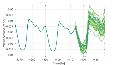
Figure 1: Collection of possible upcoming demands at a given time instant. These results were produced using the SVM model and the data in [10].

III Stochastic MPC for DWNs

In this section we define the control objectives for the controlled operation of a DWN and we formulate the stochastic MPC problem.

III-A Control objectives

We define the following three cost functions which reflect our control objectives. The economic cost quantifies the production and transportation cost

$$\ell^{w}(u_{k},k)=W_{\alpha}(\alpha_{1}+\alpha_{2,k})^{\prime}u_{k},$$ (4)

where the term $\alpha_{1}^{\prime}u_{k}$ is the water production cost, $\alpha_{2,k}^{\prime}u_{k}$ is the pumping (electricity) cost and $W_{\alpha}$ is a positive scaling factor.

The smooth operation cost is defined as

$$\ell^{\Delta}(\Delta u_{k})=\Delta u_{k}^{\prime}W_{u}\Delta u_{k},$$ (5)

where $\Delta u_{k}=u_{k}-u_{k-1}$ and $W_{u}\in\mathbb{R}^{n_{u}\times n_{u}}$ is a symmetric positive definite weight matrix. It is introduced to penalize abrupt switching of the actuators (pumps and valves).

The safety operation cost penalizes the drop of water level in the tanks below a given safety level. An elevation above this safety level ensures that there will be enough water in unforeseen cases of unexpectedly high demand and also maintains a minimum pressure for the flow of water in the network. This is given by

$$\ell^{S}(x_{k})=W_{x}\operatorname{dist}(x_{k}\mid\mathcal{C}_{s}),$$ (6)

where $\operatorname{dist}(x\mid\mathcal{C})=\inf_{y\in\mathcal{C}}\|x-y\|_{2}$ is the distance-to-set function, $\mathcal{C}_{s}=\{x\mid x\geq x_{s}\}$, and $x_{s}\in\mathbb{R}^{n_{x}}$ is the safety level and $W_{x}$ is a positive scaling factor.

These cost functions have been used in many MPC formulations in the literature [10, 2, 34]. A comprehensive discussion on the choice of these cost functions can be found in [14].

The total stage cost at a time instant $k$ is the summation of the above costs and is given by

$$\ell(x_{k},u_{k},u_{k-1},k)=\ell^{w}(u_{k},k)+\ell^{\Delta}(\Delta u_{k})+\ell^{S}(x_{k}).$$ (7)

III-B SMPC formulation

We formulate the following stochastic MPC problem with decision variables $\pi=\{u_{k+j\mid k},x_{k+j+1\mid k}\}_{j\in\mathbb{N}_{[0,N-1]}}$

$$V^{\star}(p,q,\hat{\mathbf{d}}_{k},k)=\min_{\pi}{\mathbb{E}}V(\pi,p,q,k),$$ (8a)

where $${\mathbb{E}}$$ is expectation operator and

$$V(\pi,p,q,k)=\sum_{j=0}^{N-1}\ell(x_{k+j\mid k},u_{k+j\mid k},u_{k+j-1\mid k},k{+}j),$$ (8b)

subject to the constraints

$$x_{k\mid k}=p,\ u_{k-1\mid k}=q,$$ (8c)

$$x_{k+j+1\mid k}=Ax_{k+j\mid k}+Bu_{k+j\mid k}+G_{d}d_{k+j\mid k}(\epsilon_{j}),$$

$$\qquad j\in\mathbb{N}_{[0,N-1]},\epsilon_{j}\in\Omega_{j},$$ (8d)

$$Eu_{k+j\mid k}+E_{d}d_{k+j\mid k}(\epsilon_{j})=0,j\in\mathbb{N}_{[0,N-1]},\epsilon_{j}\in\Omega_{j},$$ (8e)

$$x_{\min}\leq x_{k+j\mid k}\leq x_{\max},j\in\mathbb{N}_{[1,N]},$$ (8f)

$$u_{\min}\leq u_{k+j\mid k}\leq u_{\max},j\in\mathbb{N}_{[0,N-1]},$$ (8g)

where we stress out that the decision variables $$\{u_{k+j\mid k}\}_{j=0}^{j=N-1}$$ are required to be causal control laws of the form

$$u_{k+j\mid k}=\varphi_{k+j\mid k}(p,q,x_{k+j\mid k},u_{k+j-1\mid k},\boldsymbol{\epsilon}_{j}).$$ (8h)

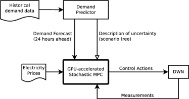
Figure 2: The closed-loop system with the proposed stochastic MPC controller running on a GPU device.

Solving the above problem would involve the evaluation of multi-dimensional integrals over an infinite-dimensional space which is computationally intractable. Hereafter, however, we shall assume that all $\Omega_{j}$, for $j\in\mathbb{N}_{[0,N-1]}$, are finite sets. This assumption will allow us to restate (8) as a finite-dimensional optimization problem.

III-C Scenario trees

A scenario tree is the structure which naturally follows from the finiteness assumption of $\Omega_{j}$ and is illustrated in Fig. 3. A scenario tree describes a set of possible future evolutions of the state of the system known as scenarios. Scenario trees can be constructed algorithmically from raw data as in [27].

Figure 3: Scenario tree describing the possible evolution of the system state along the prediction horizon: Future control actions are decided in a non-anticipative (causal) fashion; for example $u_{1}^{2}$ is decided as a function of $\epsilon_{1}^{2}$ but not of any of $\epsilon_{2}^{i}$, $i\in\mathbb{N}_{[1,\mu(3)]}$.

The nodes of a scenario tree are partitioned in stages. The (unique) node at stage $k=0$ is called root and the nodes at the last stage are the leaf nodes of the tree. We denote the number of leaf nodes by $n_{s}$. The number of nodes at stage $k$ is denoted by $\mu(k)$ and the total number of nodes of the tree is denoted by $\mu$. A path connecting the root node with a leaf node is called a scenario. Non-leaf nodes define a set of children; at a stage $j\in\mathbb{N}_{[0,N-1]}$ for $i\in\mu(j)$ the set of children of the $i$-th node is denoted by $\operatorname{child}(j,i)\subseteq\mathbb{N}_{[1,\mu(j+1)]}$. At stage $j\in\mathbb{N}_{[1,N]}$ the $i$-th node $i\in\mathbb{N}_{[1,\mu(j)]}$ is reachable from a single node at stage $k-1$ known as its ancestor which is denoted by $\operatorname{anc}(j,i)\in\mathbb{N}_{[1,\mu(j-1)]}$.

The probability of visiting a node $i$ at stage $j$ starting from the root is denoted by $p_{j}^{i}$. For all for $j\in\mathbb{N}_{N}$ we have that $\sum_{i=1}^{\mu(j)}p_{j}^{i}=1$ and for all $i\in\mathbb{N}_{[1,\mu(k)]}$ it is $\sum_{l\in\operatorname{child}(j,i)}p_{j+1}^{l}=p_{j}^{i}$.

We define the maximum branching factor at stage $j$, $b_{j}$, to be the maximum number of children of the nodes at this stage. The maximum branching factor serves as a measure of the complexity of the tree at a given stage.

III-D Reformulation as a finite-dimensional problem

We shall now exploit the above tree structure to reformulate the optimal control problem (8) as a finite-dimensional problem. The water demand, given by (3), is now modeled as

$$d_{k+j\mid k}^{i}=\hat{d}_{k+j\mid k}+\epsilon_{j}^{i},$$ (9)

for all $j\in\mathbb{N}_{[0,N-1]}$ and $i\in\mathbb{N}_{[1,\mu(j+1)]}$. The input-disturbance coupling (8e) is then readily rewritten as

$$Eu_{k+j\mid k}^{i}+E_{d}d_{k+j\mid k}^{i}=0,$$ (10)

for $j\in\mathbb{N}_{[0,N-1]}$ and $i\in\mathbb{N}_{[1,\mu(j+1)]}$.

The system dynamics is defined across the nodes of the tree by

$$x_{k+j+1\mid k}^{l} =Ax_{k+j\mid k}^{i}+Bu_{k+j\mid k}^{l}+G_{d}d_{k+j\mid k}^{l},$$ (11)

for $j\in\mathbb{N}_{[0,N-1]}$, $i\in\mathbb{N}_{[1,\mu(j)]}$ and $l\in\operatorname{child}(j,i)$, or, alternatively,

$$x_{k+j+1\mid k}^{i} =Ax_{k+j\mid k}^{\operatorname{anc}(j+1,i)}+Bu_{k+j\mid k}^{i}+G_{d}d_{k+j\mid k}^{i},$$ (12)

for $j\in\mathbb{N}_{[0,N-1]}$ and $i\in\mathbb{N}_{[1,\mu(j+1)]}$.

Now the expectation of the objective function (8b) can be derived as a summation across the tree nodes

$${\mathbb{E}}V(\pi,p,q,k)=$$

$$\quad\sum_{j=0}^{N-1}\sum_{i=1}^{\mu(j)}p_{j}^{i}\ell(x_{k+j\mid k}^{i},u_{k+j\mid k}^{i},u_{k+j-1\mid k}^{\operatorname{anc}(j,i)},k+j),$$ (13)

where $x_{k\mid k}^{1}=p$ and $u_{k-1\mid k}=q$.

In order to guarantee the recursive feasibility of the control problem, the state constraints (8f) are converted into soft constraints, that is, they are replaced by a penalty of the form

$$\ell^{d}(x)=\gamma_{d}\operatorname{dist}(x,\mathcal{C}_{1}),$$ (14)

where $\gamma_{d}$ is a positive penalty factor and $\mathcal{C}_{1}=\{x\mid x_{\min}\leq x\leq x_{\max}\}$. Using this penalty, we construct the soft state constraint penalty

$$V_{s}(\pi,p)=\sum_{j=0}^{N}\sum_{i=1}^{\mu(j)}\ell^{d}(x_{k+j\mid k}^{i}).$$ (15)

The modified, soft-constrained, SMPC problem can be now written as

$$\tilde{V}^{\star}(p,q,\hat{\mathbf{d}},k)= \min_{\pi}{\mathbb{E}}V(\pi,p,q,k)+V_{s}(\pi,p),$$ (16a)

subject to

$$x_{k\mid k}^{1}=p,\ u_{k-1\mid k}=q,$$ (16b)

$$u_{\min}\leq u_{k+j\mid k}^{i}\leq u_{\max},j\in\mathbb{N}_{[0,N-1]},i\in\mathbb{N}_{[1,\mu(j)]},$$ (16c)

and system equations (10) and (12).

IV Solution of the stochastic optimal control problem

In this section we extend the GPU-based proximal gradient method proposed in [35] to solve the SMPC problem (16). For ease of notation we will focus on the solution of the SMPC problem at $k=0$ and denote $x_{j\mid 0}=x_{j}$, $u_{j\mid 0}=u_{j}$, $\hat{d}_{j\mid 0}=\hat{d}_{j}$.

IV-A Proximal gradient algorithm

For a closed, proper extended-real valued function $g:\mathbb{R}^{n}\rightarrow\bar{\mathbb{R}}$, we define its proximal operator with parameter $\gamma>0$, $\operatorname{prox}_{\gamma g}:\mathbb{R}^{n}\rightarrow\mathbb{R}^{n}$ as [36]

$$\operatorname{prox}_{\gamma g}(v)=\operatorname*{argmin}_{x\in\mathbb{R}^{n}}\bigg{\{}g(x)+\frac{1}{2\gamma}\|x-v\|_{2}^{2}\bigg{\}}.$$ (17)

The proximal operator of many functions is available in closed form [37, 36]. When $g$ is given in a separable sum form, that is

$$g(x)=\sum_{i=1}^{\kappa}g_{i}(x_{i}),$$ (18a)

then,

$$(\operatorname{prox}_{\gamma g}(v))_{i}=\operatorname{prox}_{\gamma g_{i}}(v_{i}).$$ (18b)

This is known as the separable sum property of the proximal operator.

Let $z\in\mathbb{R}^{n_{z}}$ be a vector encompassing all states $x_{j}^{i}$ for $j\in\mathbb{N}_{[0,N]}$ and $i\in\mathbb{N}_{[1,\mu(j)]}$ and inputs $u_{j}^{i}$ for $j\in\mathbb{N}_{[0,N-1]}$, $i\in\mathbb{N}_{[1,\mu(j+1)]}$; this is the decision variable of problem (16).

Let $f:\mathbb{R}^{n_{z}}\to\bar{\mathbb{R}}$ be defined as

$$f(z) =\sum_{j=0}^{N-1}\sum_{i=1}^{\mu(j)}p_{j}^{i}(\ell^{w}(u_{j}^{i})+\ell^{\Delta}(\Delta u_{j}^{i}))$$

$$+\delta(u_{j}^{i}|\Phi_{1}(d_{j}^{i}))$$

$$+\delta(x_{j+1}^{i},u_{j}^{i},x_{j}^{\operatorname{anc}(j+1,i)}|\Phi_{2}(d_{j}^{i})),$$ (19)

where $\Delta u_{j}^{i}=u_{j}^{i}-u_{j-1}^{\operatorname{anc}(j,i)}$ and $\Phi_{1}(d)$ is the affine subspace of $\mathbb{R}^{n_{u}}$ induced by (10), that is

$$\Phi_{1}(d)=\{u:Eu+E_{d}d=0\},$$ (20)

and $\Phi_{2}(d)$ is the affine subspace of $\mathbb{R}^{2n_{x}+n_{u}}$ defined by the system dynamics (12)

$$\Phi_{2}(d)=\{(x_{k+1},x_{k},u):x_{k+1}=Ax_{k}+Bu+G_{d}d\}.$$ (21)

We define the auxiliary variables $\varsigma$ and $\zeta$ which stand for copies of the state variables $x_{j}^{i}$ — that is $\varsigma_{j}^{i}=\zeta_{j}^{i}=x_{j}^{i}$ — and the auxiliary variable $\psi$ which is a copy of input variables $\psi_{j}^{i}=u_{j}^{i}$. The reason for the introduction of these variables will be clarified in Section IV-C.

We introduce the variable $t=(\varsigma,\zeta,\psi)\in\mathbb{R}^{n_{t}}$ and define an extended real valued function $g:\mathbb{R}^{n_{t}}\to\bar{\mathbb{R}}$ as

$$g(t) =\sum_{j=0}^{N-1}\sum_{i=1}^{\mu(j)}\ell^{S}(\varsigma_{j+1}^{i})+\ell^{d}(\zeta_{j+1}^{i})+\delta(\psi_{j}^{i}|\mathcal{U}),$$ (22)

where $\mathcal{U}=\{\psi\in\mathbb{R}^{n_{u}}:u_{\min}\leq\psi\leq u_{\max}\}$.

Now the finite-dimensional optimization problem (16) can be written as:

$$\tilde{V}^{\star} =\min_{z,t}f(z)+g(t),$$ (23a)

s.t. $$Hz=t,$$ (23b)

where

$$H=\left[\begin{array}[]{cc}I_{n_{x}}&0\\ I_{n_{x}}&0\\ 0&I_{n_{u}}\end{array}\right].$$ (24)

The Fenchel dual of (23) is written as [38, Corol. 31.2.1]:

$$\tilde{D}^{\star}=\min_{y}f^{*}(-H^{\prime}y)+g^{*}(y),$$ (25)

where $y$ is the dual variable. The dual variable $y$ can be partitioned as $y=(\tilde{\varsigma}_{j}^{i},\tilde{\zeta}_{j}^{i},\tilde{\psi}_{j}^{i})$, where $\tilde{\varsigma}_{j}^{i}$, $\tilde{\zeta}_{j}^{i}$ and $\tilde{\psi}_{j}^{i}$ are the dual variables corresponding to $\varsigma_{j}^{i}$, $\zeta_{j}^{i}$ and $\psi_{j}^{i}$ respectively. We also define the auxiliary variable of state copies $\tilde{\xi}_{j}^{i}\mathrel{\mathop{:}}=(\tilde{\varsigma}_{j}^{i},\tilde{\zeta}_{j}^{i})$.

According to [39, Thm. 11.42], since function $f(z)+g(Hz)$ is proper, convex and piecewise linear-quadratic, then the primal problem (23) is feasible whenever the dual problem (25) is feasible and, furthermore, strong duality holds, i.e., $\tilde{V}^{\star}=\tilde{D}^{\star}$. Moreover, the optimal solution of (23) is given by $z^{\star}=\nabla f^{\ast}(-H^{\prime}y^{\star})$ where $y^{\star}$ is any solution of (25). Applying [39, Prop. 12.60] to $f^{*}$ and since $f$ is lower semi-continuous, proper and $\sigma$-strongly convex — as shown at the end of Appendix A — its conjugate $f^{\ast}$ has Lipschitz-continuous gradient with a constant $1/\sigma$.

An accelerated version of proximal-gradient method which was first proposed by Nesterov in [40] is applied to the dual problem. This leads to the following algorithm

$$w^{\nu} =y^{\nu}+\theta_{\nu}(\theta_{\nu-1}^{-1}-1)(y^{\nu}-y^{\nu-1}),$$ (26a)

$$z^{\nu} =\operatorname*{argmin}_{z}\{\langle z,H^{\prime}w^{\nu}\rangle+f(z)\},$$ (26b)

$$t^{\nu} =\operatorname{prox}_{\lambda^{-1}g}(\lambda^{-1}w^{\nu}+Hz^{\nu}),$$ (26c)

$$y^{\nu+1} =w^{\nu}+\lambda(Hz^{v}-t^{v}),$$ (26d)

$$\theta_{\nu+1} =\frac{1}{2}\bigg{(}\sqrt{\theta_{\nu}^{4}+4\theta_{\nu}^{2}}-\theta_{\nu}^{2}\bigg{)},$$ (26e)

starting from a dual-feasible vector $y^{0}=y^{-1}=0$ and $\theta_{0}=\theta_{-1}=1$.

In the first step (26a) we compute an extrapolation of the dual vector. In the second step (26b) we calculate the dual gradient, that is $z^{\nu}=\nabla f^{\ast}(-H^{\prime}w^{\nu})$, at the extrapolated dual vector using the conjugate subgradient theorem [38, Thm. 23.5]. The third step comprises of (26c), (26d) where we update the dual vector $y$ and in the final step of the algorithm we compute the scalar $\theta_{\nu}$ which is used in the extrapolation step.

This algorithm has a convergence rate of $\mathcal{O}(1/\nu^{2})$ for the dual iterates as well as for the ergodic primal iterate defined through the recursion $\bar{z}^{\nu}=(1-\theta_{\nu})\bar{z}^{(\nu-1)}+\theta_{\nu}z^{\nu}$, i.e., a weighted average of the primal iterates [41].

IV-B Computation of primal iterate

The most critical step in the algorithm is the computation of $z^{\nu}$ which accounts for most of the computation time required by each iteration. This step boils down to the solution of an unconstrained optimization problem by means of dynamic programming where certain matrices (which are independent of $w^{\nu}$) can be computed once before we run the algorithm to facilitate the online computations. These are (i) the vectors $\beta_{j}^{i},\hat{u}_{j}^{i},e_{j}^{i}$ which are associated with the update of the time-varying cost (see Appendix A) and (ii) the matrices $\Lambda,\Phi,\Psi,\bar{B}$ (see Appendix B). The latter are referred to as the factor step of the algorithm and matrices $\Lambda,\Phi,\Psi$ and $\bar{B}$ are independent of the complexity of the scenario tree.

The computation of $z^{\nu}$ at each iteration of the algorithm requires the computation of the aforementioned matrices and is computed using Algorithm 1 to which we refer as the solve step. Computations involved in the solve step are merely matrix-vector multiplications. As the algorithm traverses the nodes of the scenario tree stage-wise backwards (from stage $N-1$ to stage $0$), computations across the nodes at a given stage can be performed in parallel. Hardware such as GPUs which enable us to parallelizable such operations lead to a great speed-up as we demonstrate in Section V.

Algorithm 1 Solve step

0:  Output of the factor step (See Appendices A and B), i.e., $\Lambda,\Phi,\Psi,\bar{B},\hat{u}_{j}^{i},\beta_{j}^{i},e_{j}^{i}$, $p$, $q$ and $w^{\nu}=(\tilde{\varsigma}_{j}^{i},\tilde{\zeta}_{j}^{i},\tilde{\psi}_{j}^{i})$.

  $q_{N}^{i}\leftarrow 0$, and $r_{N}^{i}\leftarrow 0,\forall i\in\mathbb{N}_{[1,n_{s}]}$,

  for $j=N-1,\ldots,0$ do

     for $i=1,\ldots,\mu(k)$ do {in parallel}

        $\sigma_{j}^{l}\leftarrow r_{j+1}^{l}+\beta_{j}^{l},\forall l\in\operatorname{child}(j,i)$

        $v_{j}^{l}\leftarrow\frac{1}{2p_{j}^{l}}\left(\Phi_{j}^{l}(\tilde{\xi}_{j}^{l}+q_{j+1}^{l})+\Psi_{j}^{l}\tilde{\psi}_{j}^{l}+\Lambda_{j}^{l}\sigma_{j}^{l}\right),$  $\forall l\in\operatorname{child}(j,i)$

        $r_{j}^{i}\leftarrow\sum_{l\in\operatorname{child}(j,i)}\sigma_{j}^{l}+\bar{B}^{\prime}(\tilde{\xi}_{j}^{l}+q_{j+1}^{l})+L\tilde{\psi}_{j}^{l}$

        $q_{j}^{i}\leftarrow A^{\prime}\sum_{l\in\operatorname{child}(j,i)}\tilde{\xi}_{j}^{l}+q_{j+1}^{l}$

     end for

  end for

  $x_{0}^{1}\leftarrow p$, $u_{-1}\leftarrow q$,

  for $j=0,\ldots,N-1$ do

     for $i=1,\ldots,\mu(k)$ do {in parallel}

        $v_{j}^{i}\leftarrow v_{j-1}^{\operatorname{anc}(j,i)}+v_{j}^{i}$

        $u_{j}^{i}\leftarrow Lv_{j}^{i}+\hat{u}_{j}^{i}$

        $x_{j+1}^{i}\leftarrow Ax_{j}^{\operatorname{anc}(j,i)}+\bar{B}v_{j}^{i}+e_{j}^{i}$

     end for

  end for

  return  $\{x_{j}^{i}\}_{j=1}^{N}$, $\{u_{j}^{i}\}_{j=0}^{N-1}$

IV-C Computation of dual iterate

Function $g$ given in (22) is given in the form of a separable sum

$$g(t)=g(\varsigma,\zeta,\psi)=g_{1}(\varsigma)+g_{2}(\zeta)+g_{3}(\psi),$$ (27)

where

$$g_{1}(\varsigma) =\sum_{j=0}^{N-1}\sum_{i=1}^{\mu(j)}\ell^{S}(\varsigma_{j+1}^{i}),$$ (28a)

$$g_{2}(\zeta) =\sum_{j=0}^{N-1}\sum_{i=1}^{\mu(j)}\ell^{d}(\zeta_{j+1}^{i}),$$ (28b)

$$g_{3}(\psi) =\sum_{j=0}^{N-1}\sum_{i=1}^{\mu(j)}\delta(\psi_{j}^{i}\mid\mathcal{U}).$$ (28c)

Functions $g_{1}(\cdot)$ and $g_{2}(\cdot)$ are in turn separable sums of distance functions from a set and $g_{3}(\cdot)$ is an indicator function. Their proximal mappings can be easily computed as in Appendix C and essentially are element-wise operations on the vector $t$ that can be fully parallelized.

IV-D Preconditioning and choice of $\lambda$

First-order methods are known to be sensitive to scaling and preconditioning can remarkably improve their convergence rate. Various preconditioning method such as [42, 43] have been proposed in the literature. Here, we employ a simple diagonal preconditioning which consists in computing a diagonal matrix $\tilde{H}_{D}$ with positive diagonal entries which approximates the dual Hessian $H_{D}$ and use $\tilde{H}^{-1/2}_{D}$ to scale the dual vector [44, 2.3.1]. Since the uncertainty does not affect the dual Hessian, we take this preconditioning matrix for a single branch of the scenario tree and use it to scale all dual variables.

In a similar way, we compute the parameter $\lambda$. We choose $\lambda=1/L_{H_{D}}$ where $L_{H_{D}}$ is the Lipschitz constant of the dual gradient which is computed as $\|H\|^{2}/\sigma$ as in [44]. It again suffices to perform the computation for a single branch of the scenario tree.

IV-E Termination

The termination conditions for the above algorithm are based on the ones provided in [41]. However, rather than checking these conditions at every iteration, we perform always a fixed number of iterations which is dictated by the sampling time. We may then check the quality of the solution a posteriori in terms of the duality gap and the term $\|Hz^{\nu}-t^{\nu}\|_{\infty}$.

V Case study: The Barcelona DWN

We now apply the proposed control methodology to the drinking water network of the city of Barcelona using the data found in [2, 10]. The topology of the network is presented in Figure 4. The system model consists of $63$ states corresponding to the level of water in each tank, $114$ control inputs which are pumping actions and valve positions, $88$ demand nodes and $17$ junctions. The prediction horizon is $N=24$ with sampling time of $1$ hour. The future demands are predicted using the SVM time series model developed in [10].

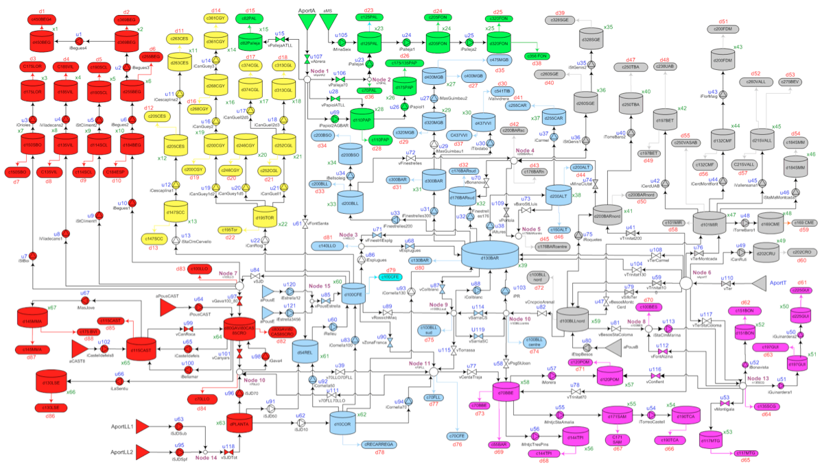
Figure 4: Structure of the DWN of Barcelona.

V-A Performance of GPU-accelerated algorithm

Accelerated proximal gradient (APG) was implemented in CUDA-C v6.0 and the matrix-vector computations were performed using cuBLAS. We compared the GPU-based implementation with the interior-point solver of Gurobi. Active-set algorithms exhibited very poor performance and we did not include the respective results.

All computations on CPU were performed on a $4\times 2.60\mathrm{GHz}$ Intel i5 machine with $8\mathrm{GB}$ of RAM running 64-bit Ubuntu v14.04 and GPU-based computations were carried out on a NVIDIA Tesla C2075.

The dependence of the computational time on the size of the scenario tree is reported in the Figure 5 where it can be noticed that there is speed-up of $10\times$ to $25\times$ in the computational times with CUDA-APG compared to Gurobi. Furthermore, the speed-up increases with the number of scenarios.

The optimization problems we are solving here are of noticeably large size. Indicatively, the scenario tree with $493$ scenarios counts approximately $2.52$ million dual decision variables ($1.86$ million primal variables) and while Gurobi requires $1329s$ to solve it, our CUDA implementation solves it in $58.8s$; this corresponds to a speed-up of $22.6\times$.

In all of our simulations we obtained a sequence of control actions across the tree nodes $U^{\star}_{apg}=\{u_{j}^{i}\}$ which was, element-wise, within $\pm 0.029m^{3}/s$ ($1.9\%$) from the solution produced by Gurobi. The maximum primal residual was $\|Hx-z\|_{\infty}=1.7446$. Moreover, we should note that the control action $u_{0}^{\star}$ computed by APG with $500$ iterations was consistently within $\pm 0.0025m^{3}/s$ ($0.08\%$) from the Gurobi solution. Given that only $u_{0}^{\star}$ is applied to the system while all other control actions $u_{j}^{i}$ for $j\in\mathbb{N}_{[1,N-1]}$ and $i\in\mathbb{N}_{[1,\mu(j)]}$ are discarded, $500$ iterations are well sufficient for convergence.

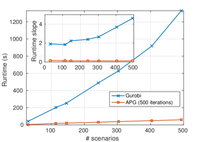
Figure 5: Runtime of the CUDA implementation against the number of scenarios considered in the optimization problem. Comparison with the runtimes of Gurobi.

V-B Closed-loop performance

In this section we analyse the performance of SMPC with different scenario-trees. This analysis is carried for a period of 7 days ($H_{s}=168$) from 1${}^{\text{st}}$ to 8${}^{\text{th}}$ July 2007. Here, we compare the operational cost and the quality of service of various scenario-tree structures.

The weighting matrices in the operational cost are chosen as $W_{\alpha}=2\cdot 10^{4}$, $W_{u}=10^{5}\cdot I$ and $W_{x}=10^{7}$, respectively and $\gamma_{d}=5\cdot 10^{7}$. The demand is predicted using SVM model presented in [10]. The steps involved in SMPC using GPU based APG in closed-loop is summarized in Algorithm 2.

Algorithm 2 Closed-loop of DWN with SMPC with proximal-operator

0:  Scenario-tree, current state measurement $x_{0}$ and previous control $u_{-1}$.

  Compute $\Lambda$, $\Phi$, $\Psi$ and $\bar{B}$ as in Appendix B

  Precondition the original optimization problem and compute $\lambda$ as in Section IV-D.

  loop

     Step 1. Predict the future water demands $\hat{\mathbf{d}}_{k}$ using current and past demand data.

     Step 2. Compute $\hat{u}_{j}^{i}$, $\beta_{j}^{i},e_{j}^{i}$ as in Appendix A.

     Step 3. Solve the optimization problem using APG on GPU using iteration (26) and Algorithm 1.

     Step 4. Apply $u_{0}^{1}$ to the system, update the previous $u_{-1}=u_{0}^{1}$

  end loop

For the performance assessment of the proposed control methodology we used various controllers summarized in Table I. The corresponding computational times are presented in Figure 5.

Controller	$b_{k}$	scenarios	primal variables	dual variables
CE-MPC	$1$	$1$	$4248$	$5760$
SMPC1	$[3,2]$	$6$	$24072$	$32540$
SMPC2	$[6,5]$	$30$	$118059$	$160080$
SMPC3	$[6,5,5]$	$114$	$430287$	$583440$
SMPC4	$[8,5,5]$	$146$	$551355$	$747600$
SMPC5	$[10,8,5]$	$242$	$915621$	$1241520$
SMPC6	$[12,8,5]$	$303$	$1145544$	$1553280$
SMPC7	$[12,8,8]$	$404$	$1520961$	$2062320$
SMPC8	$[12,10,8]$	$493$	$1856022$	$2516640$

TABLE I: Various controllers used to assess the closed-loop performance of the proposed methodology. The numbers in the bracket denote the first maximum branching factors, $b_{j}$, of the scenario tree while all subsequent branching factors are assumed to be equal to $1$.

To assess the performance of closed-loop operation of the SMPC-controlled network we used the key performance indicators (KPIs) reported in [45, 3]. For a simulation time length $H_{s}$ the performance indicators are computed by

$$\mathrm{KPI}_{E}=\frac{1}{H_{s}}\sum_{k=1}^{H_{s}}(\alpha_{1}+\alpha_{2,k})^{\prime}|u_{k}|,$$ (29a)

$$\mathrm{KPI}_{\Delta U}=\frac{1}{H_{s}}\sum_{k=1}^{H_{s}}\|\Delta u_{k}\|^{2},$$ (29b)

$$\mathrm{KPI}_{S}=\sum_{k=1}^{H_{s}}\|[x_{s}-x_{k}]_{+}\|_{1},$$ (29c)

$$\mathrm{KPI}_{R}=\frac{\|x_{s}\|_{1}}{\frac{1}{H_{s}}\sum_{k=1}^{H_{s}}\|x_{k}\|_{1}}\times 100\%.$$ (29d)

$\mathrm{KPI}_{E}$ is the average economic cost, $\mathrm{KPI}_{\Delta U}$ measures the average smoothness of the control actions, $\mathrm{KPI}_{S}$ corresponds to the total amount of water used from storage and $\mathrm{KPI}_{R}$ is the percentage of the safety volume $x_{s}$ contained into the average volume of water.

Controller	$\mathrm{KPI}_{E}$	$\mathrm{KPI}_{\Delta U}$	$\mathrm{KPI}_{S}$	$\mathrm{KPI}_{R}$
CE-MPC	$\mathbf{1801.4}$	$\mathbf{0.2737}$	$\mathbf{6507.7}$	$64.89\%$
SMPC1	$1633.5$	$0.3896$	$1753.7$	$\mathbf{67.96\%}$
SMPC2	$\mathbf{1549.7}$	$0.4652$	$2264.0$	$61.81\%$
SMPC3	$1574.0$	$0.4135$	$1360.0$	$49.65\%$
SMPC4	$1583.2$	$0.4088$	$885.7$	$48.13\%$
SMPC5	$1597.3$	$0.4470$	$508.5$	$46.05\%$
SMPC6	$1606.3$	$\mathbf{0.4878}$	$\mathbf{302.3}$	$\mathbf{44.93\%}$

TABLE II: KPIs for performance analysis of the DWN with different controllers. The lowest and the highest in each of the indicator is highlighted. The economical benefit and risk is presented with terms of number of scenarios

V-B1 Risk vs Economic utility

Figure 6 illustrates the trade-off between economic and safe operation: The more scenarios we use to describe the distribution of demand prediction error, the safer the closed-loop operation becomes as it is reflected by the decrease of KPI_S. Stochastic MPC leads to a significant decrease of economic cost compared to the certainty-equivalence approach, however, the safer we require the operation to be, the higher the operating cost we should expect.

V-B2 Quality of service

A measure of the reliability and quality-of-service of the network is $\mathrm{KPI}_{S}$ which reflects the tendency of water levels to drop under the safety storage levels. As expected, the CE-MPC controller leads to the most unsafe operation, whereas SMPC₆ leads to the lowest value.

V-B3 Network utility

Network utility is defined as the ability to utilize the water in the tanks to meet the demands rather than pumping additional water and is quantified by $\mathrm{KPI}_{R}$. In Table II, we see the dependence of $\mathrm{KPI}_{R}$ on the number of scenarios of the tree. $\mathrm{KPI}_{R}$ remains always within reasonable limits; on average we operate away from the safety storage limit. The decrease in $\mathrm{KPI}_{R}$ on may observe is because as more scenarios are employed, the more accurate the representation of uncertainty becomes and the system does not need to operate, on average, too far away from $x_{s}$.

V-B4 Smooth operation

We may notice that the introduction of more scenarios results in an increase in $\mathrm{KPI}_{\Delta U}$. Then, the controller becomes more responsive to accommodate the need for a less risky operation, although the value of $\mathrm{KPI}_{\Delta U}$ is not greatly affected by number of scenarios.

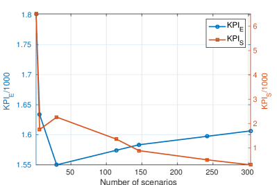
Figure 6: The figure shows the trade-off between risk and economic utility in terms of scenarios. The KPI_E represent the economical utility and KPI_S shows the risk of violation.

Figure 7: A pumping action using SMPC₄ (expressed in $\%$ of $u_{\max}$) and the corresponding weighted time-varying cost $W_{\alpha}\alpha_{2,k}$ in economic units.

V-C Implementation details

At every time instant $k$ we need to load onto the GPU the state measurement and a sequence of demand predictions (see Figure 2), that is ${\hat{\mathbf{d}}}_{k}$. This amounts to $8.4kB$ and is rapidly uploaded on the GPU (less than $0.034ms$). In case we need to update the scenario-tree values, that is $\boldsymbol{\epsilon}_{k}$, and for the case of $\mathrm{SMPC}_{8}$ we need to upload $3.52MB$ which is done in $3.74ms$. Therefore, the time needed to load these data on the GPU is not a limiting factor.

VI Conclusions

In this paper we have presented a framework for the formulation of a stochastic model predictive control problem for the operational management of drinking water networks and we have proposed a novel approach for the efficient numerical solution of the associated optimization problem on a GPU.

We demonstrated the computational feasibility of the algorithm and the benefits for the operational management of the system in terms of performance (which we quantified using certain KPIs from the literature).

Appendix A Elimination of input-disturbance coupling

In this section we discuss how the input-disturbance equality constraints can be eliminated by a proper change of input variables and we compute the parameters $\beta_{j}^{i},\hat{u}_{j}^{i},e_{j}^{i}$ $\forall i\in\mu(j),j\in\mathbb{N}_{N}$ which are then provided as input to Algorithm 1. These depend on the nominal demand forecasts $\hat{d}_{k+j\mid k}$ and on the time-varying economic cost parameters $\alpha_{2,k+j}$ for $j\in\mathbb{N}_{[0,N-1]}$, therefore, they need to be updated at every time instant $k$.

The affine space $\Phi_{1}(d)$ introduced in (20) can be written as

$$\Phi_{1}(d)=\{v\in\mathbb{R}^{n_{v}}:u=Lv+\hat{u}(d)\},$$ (30)

where $L\in\mathbb{R}^{n_{u}\times n_{v}}$ is a full rank matrix whose range spans the nullspace of $E$, i.e., for every $v\in\mathbb{R}^{n_{v}}$, we have $Lv$ is in the kernel of $E$ and $\hat{u}(d)$ satisfies $E\hat{u}(d)+E_{d}d=0$.

Substituting $u_{j}^{i}=Lv_{j}^{i}+\hat{u}_{j}^{i},\forall i\in\mu(j),j\in\mathbb{N}_{N}$ in the dynamics $\Phi_{2}(d)$ in (21) gives

$$\Phi_{2}(d)= \{(x_{j+1},x_{j},v):x_{j+1}=Ax_{j}+\bar{B}v+e,$$

$$\bar{B}=BL,e=B\hat{u}+G_{d}d\},$$ (31)

and we define

$$e_{j}^{i}=B\hat{u}_{j}^{i}+G_{d}d_{j}^{i}.$$ (32)

Now the cost in (19) is transformed as:

$$\sum_{j=0}^{N-1}\sum_{i=1}^{\mu(j)}p_{j}^{i}(\ell^{w}(u_{j}^{i})+\ell^{\Delta}(\Delta u_{j}^{i})) =$$

$$\sum_{j=0}^{N-1}\sum_{i=1}^{\mu(j)}p_{j}^{i}(\ell^{w}(v_{j}^{i})+\ell^{\Delta}(\Delta v_{j}^{i},\hat{u}_{j}^{i})),$$ (33)

where

$$\hat{R} =W_{u}L,$$ (34a)

$$\bar{R} =L^{\prime}\hat{R},$$ (34b)

$$\bar{\alpha}_{j} =W_{\alpha}(\alpha_{1}+\alpha_{2,j+k})L,$$ (34c)

$$\ell^{w}(v_{j}^{i}) =\bar{\alpha}_{j}^{\prime}v_{j}^{i},$$ (34d)

$$\Delta v_{j}^{i} =v_{j}^{i}-v_{j-1}^{\operatorname{anc}(j,i)},$$ (34e)

$$\Delta\hat{u}_{j}^{i} =\hat{u}_{j}^{i}-\hat{u}_{j-1}^{\operatorname{anc}(j,i)},$$ (34f)

$$\ell^{\Delta}(\Delta v_{j}^{i},\Delta\hat{u}_{j}^{i}) =\Delta v_{j}^{i}\bar{R}\Delta v_{j}^{i}+2\Delta\hat{u}_{j}^{i\prime}\hat{R}\Delta v_{j}^{i}.$$ (34g)

By substituting and expanding $\Delta v_{j}^{i}$ and $\Delta\hat{u}_{j}^{i}$ in $\ell^{\Delta}(\Delta v_{j}^{i},\Delta\hat{u}_{j}^{i})$ the cost in (34g) becomes

$$\sum_{j=0}^{N-1}\sum_{i=1}^{\mu(j)}p_{j}^{i}(\ell^{w}(u_{j}^{i})+\ell^{\Delta}(\Delta u_{j}^{i}))=$$

$$\sum_{j=0}^{N-1}\sum_{i=1}^{\mu(j)}\bar{p}_{j}^{i}v_{j}^{i\prime}\bar{R}v_{j}^{i}-2p_{j}^{i}v_{j-1}^{\operatorname{anc}(j,i)\prime}\bar{R}v_{j}^{i}+\beta_{j}^{i\prime}v_{j}^{i},$$ (35)

where

$$\bar{p}_{j}^{i} =p_{j}^{i}+\sum_{l\in\operatorname{child}(j,i)}p_{j+1}^{l},$$ (36a)

$$\beta_{j}^{i} =p_{j}^{i}\bar{\alpha}_{j}+2p_{j}^{i}\hat{R}\Big{(}\bar{p}_{j}^{i}\hat{u}_{j}^{i}-\hat{u}_{j-1}^{\operatorname{anc}(j,i)}-$$

$$\quad\sum_{l\in\operatorname{child}(j,i)}p_{j+1}^{l}\hat{u}_{j+1}^{l}\Big{)}.$$ (36b)

Now $\hat{u}_{j}^{i}$, $e_{j}^{i}$, $\beta_{j}^{i}$ are calculated from (30), (32) and (36b) respectively. Using our assumption that $L$ is full-rank, we can see that $\bar{R}$ is a positive definite and symmetric matrix, therefore, $f$ is strongly convex.

Appendix B Factor step

Algorithm 1 solves the unconstrained minimization problem (26b), that is

$$z^{\star}=\operatorname*{argmin}_{z}\{\langle z,H^{\prime}y\rangle+f(z)\},$$ (37)

where $z=\{x_{j}^{i},u_{j}^{i}\}$, $y=\{\tilde{\varsigma}_{j}^{i},\tilde{\zeta}_{j}^{i},\tilde{\psi}_{j}^{i}\}$ for $i\in\mathbb{N}_{[1,\mu(j)]}$ and $j\in\mathbb{N}_{[0,N]}$, $f(z)$ is given by (19) and $H$ is given by (24). Substituting $H$ the optimization problem becomes

$$z^{\star} =\operatorname*{argmin}_{z}\sum_{j=0}^{N-1}\sum_{i=1}^{\mu(j)}p_{j}^{i}(\ell^{w}(u_{j}^{i})+\ell^{\Delta}(\Delta u_{j}^{i}))$$

$$\qquad+\tilde{\xi}_{j}^{i\prime}x_{j}^{i}+\tilde{\psi}_{j}^{i\prime}u_{j}^{i}+\delta(u_{j}^{i}|\Phi_{1}(d_{j}^{i}))$$

$$\qquad+\delta(x_{j+1}^{i},u_{j}^{i},x_{j}^{\operatorname{anc}(j+1,i)}|\Phi_{2}(d_{j}^{i})),$$ (38)

where $\tilde{\xi}_{j}^{i}\mathrel{\mathop{:}}=(\tilde{\varsigma}_{j}^{i},\tilde{\zeta}_{j}^{i})$.

The input-disturbance coupling constraints imposed by $\delta(u_{j}^{i}|\Phi_{1}(d_{j}^{i}))$ in the above problem are eliminated as discussed in Appendix A. This changes the input variable from $u_{j}^{i}$ to $v_{j}^{i}$ given by (30) and the cost function as in (A). We, therefore, replace the decision variable $z$ with $\bar{z}\mathrel{\mathop{:}}=\{x_{j}^{i},v_{j}^{i}\}$ and the optimization problem (B) reduces to

$$\bar{z}^{\star} =\operatorname*{argmin}_{\bar{z}}\sum_{j=0}^{N-1}\sum_{i=1}^{\mu(j)}\bar{p}_{j}^{i}v_{j}^{i\prime}\bar{R}v_{j}^{i}-2p_{j}^{i}v_{j-1}^{\operatorname{anc}(j,i)\prime}\bar{R}v_{j}^{i}$$

$$\qquad+\beta_{j}^{i\prime}v_{j}^{i}+\tilde{\xi}_{j}^{i\prime}x_{j+1}^{j}+\tilde{\psi}_{j}^{i\prime}Lv_{j}^{i}$$

$$\qquad+\delta(x_{j+1}^{i},v_{j}^{i},x_{j}^{\operatorname{anc}(k,i)}|\Phi_{2}(d_{j}^{i})),$$ (39)

where $u_{j}^{i}=Lv_{j}^{i}+\hat{u}_{j}^{i}$.

The above problem is an unconstrained optimization problem with quadratic stage cost which is solved using dynamic programming [46]. This method transforms the complex problem into a sequence of sub-problems solved at each stage.

Using dynamic programming we find that the transformed control actions $v_{j}^{i\star}$ have to satisfy

$$v_{j}^{i\star} =v_{j-1}^{\operatorname{anc}(j,i)}+\frac{1}{2p_{j}^{i}}\big{(}\Phi(\tilde{\xi}_{j}^{i}+q_{j+1}^{i})+\Psi\tilde{\psi}_{j}^{i}$$

$$+\Lambda(\beta_{j}^{i}+r_{j+1}^{i})\big{)},$$ (40)

where

$$\Lambda =-\bar{R}^{-1},$$ (41a)

$$\Phi =\Lambda\bar{B}^{\prime},$$ (41b)

$$\Psi =\Lambda L.$$ (41c)

Matrix $\bar{R}$ is symmetric and positive definite, therefore, we can compute once its Cholesky factorization so that we obviate the computation of its inverse.

The $q_{j+1}^{i}$, $r_{j+1}^{i}$ in (40) correspond to the linear cost terms in the cost-to-go function at node $i$ of stage $j+1$. At stage $j$, these terms are updated by substituting the $v_{j}^{i\star}$ as:

$$r_{j}^{s} =\sum_{l\in\operatorname{child}(j-1,s)}\sigma_{j}^{l}+\bar{B}^{\prime}(\tilde{\xi}_{j}^{l}+q_{j+1}^{l})+L\tilde{\psi}_{j}^{l},$$ (42a)

$$q_{j}^{s} =A^{\prime}\sum_{l\in\operatorname{child}(j-1,s)}\tilde{\xi}_{j}^{l}+q_{j+1}^{l},$$ (42b)

where $s=\operatorname{anc}(j,i)$.

Equations (40) and (42) form the solve step as in Algorithm 1. Matrices $\Lambda$, $\Phi$ and $\Psi$ are required to be computed once.

Appendix C Proximal operators

Function $g$ in (27) is a separable sum of distance and indicator functions and its proximal is computed according to (18). The proximal operator of the indicator of a convex closed set $C$, that is

$$\chi_{C}(x)=\begin{cases}0,&\text{ if }x\in\mathcal{C}\\ +\infty,&\text{ otherwise }\end{cases}$$

is the projection operator onto $C$, i.e.,

$$\operatorname{prox}_{\lambda\chi_{C}}(v)=\operatorname{proj}_{\mathcal{C}}(v)=\operatorname*{argmin}_{y\in C}\|v-y\|,$$ (43)

When $g$ is the distance function from a convex closed set $C$, that is

$$g(x)= \mu\operatorname{dist}(x\mid\mathcal{C})=\inf_{y\in\mathcal{C}}\mu\|x-y\|$$

$$= \mu\|x-\operatorname{proj}_{\mathcal{C}}(x)\|.$$

Then proximal operator of $g$ given by [37]

$$\operatorname{prox}_{\lambda g}{(v)}=\begin{cases}x+\frac{\operatorname{proj}_{\mathcal{C}}(x)-x}{\operatorname{dist}(x\mid\mathcal{C})},&\text{ if }\operatorname{dist}(x\mid\mathcal{C})>\lambda\mu\\ \operatorname{proj}_{\mathcal{C}}(x),&\text{ otherwise }\end{cases}$$

References

- [1] V. Havlena, P. Trnka, and B. Sheridan, “Management of complex water networks,” in The Impact of Control Technology (T. Samad and A. Annaswamy, eds.), IEEE Control Systems Society, 2nd ed., 2014. available at www.ieeecss.org.
- [2] J. Grosso, C. Ocampo-Martínez, V. Puig, and B. Joseph, “Chance-constrained model predictive control for drinking water networks,” Journal of Process Control, vol. 24, no. 5, pp. 504 – 516, 2014.
- [3] J. Grosso, J. Maestre, C. Ocampo-Martinez, and V. Puig, “On the assessment of tree-based and chance-constrained predictive control approaches applied to drinking water networks,” in 19th IFAC Conference, (Cape town, South Africa), pp. 6240–6245, Aug. 2014.
- [4] A. Nemirovski and A. Shapiro, “Convex approximations of chance constrained programs,” SIAM Journal on Optimization, vol. 17, no. 4, pp. 969–996, 2006.
- [5] J. Creasy, “Pump scheduling in water supply: More than a mathematical problem,” Computer Applications in Water Supply, vol. 2, pp. 279–289, 1998.
- [6] U. Zessler and U. Shamir, “Optimal operation of water distribution systems,” Journal of Water Resources Planning and Management, vol. 115, no. 6, pp. 735–752, 1989.
- [7] G. Yu, R. Powell, and M. Sterling, “Optimized pump scheduling in water distribution systems,” Journal of Optimization Theory and Applications, vol. 83, no. 3, pp. 463–488, 1994.
- [8] A. Bagirov, A. Barton, H. Mala-Jetmarova, A. A. Nuaimat, S. Ahmed, N. Sultanova, and J. Yearwood, “An algorithm for minimization of pumping costs in water distribution systems using a novel approach to pump scheduling,” Mathematical and Computer Modelling, vol. 57, no. 3–4, pp. 873 – 886, 2013.
- [9] G. McCormick and R. Powell, “Derivation of near-optimal pump schedules for water distribution by simulated annealing,” Journal of the Operational Research Society, vol. 55, pp. 728–736, July 2004.
- [10] A. Sampathirao, J. Grosso, P. Sopasakis, C. Ocampo-Martinez, A. Bemporad, and V. Puig, “Water demand forecasting for the optimal operation of large-scale drinking water networks: The Barcelona case study,” in 19th IFAC World Congress, pp. 10457–10462, 2014.
- [11] C. Ocampo-Martinez, V. Puig, G. Cembrano, R. Creus, and M. Minoves, “Improving water management efficiency by using optimization-based control strategies: the barcelona case study,” Water Science and Technology: Water Supply, vol. 9, no. 5, pp. 565–575, 2009.
- [12] M. Bakker, J. H. G. Vreeburg, L. J. Palmen, V. Sperber, G. Bakker, and L. C. Rietveld, “Better water quality and higher energy efficiency by using model predictive flow control at water supply systems,” Journal of Water Supply: Research and Technology - Aqua, vol. 62, no. 1, pp. 1–13, 2013.
- [13] S. Leirens, C. Zamora, R. Negenborn, and B. De Schutter, “Coordination in urban water supply networks using distributed model predictive control,” in American Control Conference (ACC), 2010, (Baltimore, USA), pp. 3957–3962, June 2010.
- [14] C. Ocampo-Martinez, V. Fambrini, D. Barcelli, and V. Puig, “Model predictive control of drinking water networks: A hierarchical and decentralized approach,” in American Control Conference (ACC), 2010, (Baltimore, USA), pp. 3951–3956, June 2010.
- [15] G. S. Sankar, S. M. Kumar, S. Narasimhan, S. Narasimhan, and S. M. Bhallamudi, “Optimal control of water distribution networks with storage facilities,” Journal of Process Control, vol. 32, pp. 127 – 137, 2015.
- [16] V. Tran and M. Brdys, “Optimizing control by robustly feasible model predictive control and application to drinking water distribution systems,” in Artificial Neural Networks – ICANN 2009 (C. Alippi, M. Polycarpou, C. Panayiotou, and G. Ellinas, eds.), vol. 5769 of Lecture Notes in Computer Science, pp. 823–834, Springer Berlin Heidelberg, 2009.
- [17] A. Goryashko and A. Nemirovski, “Robust energy cost optimization of water distribution system with uncertain demand,” Automation and Remote Control, vol. 75, no. 10, pp. 1754–1769, 2014.
- [18] J. Watkins, D. and D. McKinney, “Finding robust solutions to water resources problems,” Journal of Water Resources Planning and Management, vol. 123, no. 1, pp. 49–58, 1997.
- [19] M. Cannon, B. Kouvaritakis, and X. Wu, “Probabilistic constrained mpc for multiplicative and additive stochastic uncertainty,” Automatic Control, IEEE Transactions on, vol. 54, pp. 1626–1632, July 2009.
- [20] D. Bernardini and A. Bemporad, “Stabilizing model predictive control of stochastic constrained linear systems,” Automatic Control, IEEE Transactions on, vol. 57, pp. 1468–1480, June 2012.
- [21] D. van Hessem and O. Bosgra, “A conic reformulation of model predictive control including bounded and stochastic disturbances under state and input constraints,” in Decision and Control, 2002, Proceedings of the 41st IEEE Conference on, vol. 4, (Las Vegas, USA), pp. 4643–4648 vol.4, Dec 2002.
- [22] D. Bertsimas and D. Brown, “Constrained stochastic LQC: A tractable approach,” Automatic Control, IEEE Transactions on, vol. 52, pp. 1826–1841, Oct 2007.
- [23] G. Calafiore and M. Campi, “The scenario approach to robust control design,” Automatic Control, IEEE Transactions on, vol. 51, pp. 742–753, May 2006.
- [24] M. C. Campi, S. Garatti, and M. Prandini, “The scenario approach for systems and control design,” Annual Reviews in Control, vol. 33, no. 2, pp. 149 – 157, 2009.
- [25] M. Prandini, S. Garatti, and J. Lygeros, “A randomized approach to stochastic model predictive control,” in Decision and Control (CDC), 2012 IEEE 51st Annual Conference on, (Maui, Hawaii, USA), pp. 7315–7320, Dec 2012.
- [26] A. Shapiro, D. Dentcheva, and A. Ruszczynski, Lectures on Stochastic Programming: Modeling and Theory. Philadelphia: Society for Industrial and Applied Mathematics, 2009.
- [27] H. Heitsch and W. Römisch, “Scenario tree modeling for multistage stochastic programs,” Mathematical Programming, vol. 118, no. 2, pp. 371–406, 2009.
- [28] M. McCool, “Signal processing and general-purpose computing and gpus [exploratory dsp],” Signal Processing Magazine, IEEE, vol. 24, pp. 109–114, May 2007.
- [29] R. Benenson, M. Mathias, R. Timofte, and L. Van Gool, “Pedestrian detection at 100 frames per second,” in Computer Vision and Pattern Recognition (CVPR), 2012 IEEE Conference on, pp. 2903–2910, June 2012.
- [30] H. Jang, A. Park, and K. Jung, “Neural network implementation using cuda and openmp,” in Digital Image Computing: Techniques and Applications (DICTA), 2008, pp. 155–161, Dec 2008.
- [31] A. Guzhva, S. Dolenko, and I. Persiantsev, Artificial Neural Networks – ICANN 2009: 19th International Conference, Limassol, Cyprus, September 14-17, 2009, Proceedings, Part I, ch. Multifold Acceleration of Neural Network Computations Using GPU, pp. 373–380. Berlin, Heidelberg: Springer Berlin Heidelberg, 2009.
- [32] S. Miyaoka and M. Funabashi, “Optimal control of water distribution systems by network flow theory,” Automatic Control, IEEE Transactions on, vol. 29, pp. 303–311, Apr 1984.
- [33] Y. Wang, C. Ocampo-Martinez, V. Puig, and J. Quevedo, “Gaussian-process-based demand forecasting for predictive control of drinking water networks,” in Proceedings of the 9th International Conference on Critical Information Infrastructures Security (CRITIS), (Limassol (Cyprus)), 2014.
- [34] S. Cong Cong, S. Puig, and G. Cembrano, “Combining CSP and MPC for the operational control of water networks: Application to the Richmond case study,” in 19th IFAC World Congress, (Cape Town), pp. 6246–6251, 2014.
- [35] A. Sampathirao, P. Sopasakis, A. Bemporad, and P. Patrinos, “Distributed solution of stochastic optimal control problems on GPUs,” in 54 IEEE Conf. Decision and Control, (Osaka, Japan), Dec 2015.
- [36] N. Parikh and S. Boyd, “Proximal algorithms,” Found. Trends Optim., vol. 1, pp. 127–239, jan 2014.
- [37] P. Combettes and J.-C. Pesquet, “Proximal splitting methods in signal processing,” 2010. arXiv:0912.3522v4.
- [38] R. Rockafellar, Convex analysis. Princeton university press, 1972.
- [39] R. Rockafellar and J. Wets, Variational analysis. Berlin: Springer-Verlag, 3rd ed., 2009.
- [40] Y. Nesterov, “A method of solving a convex programming problem with convergence rate ,” Soviet Mathematics Doklady, vol. 72, no. 2, pp. 372–376, 1983.
- [41] P. Patrinos and A. Bemporad, “An accelerated dual gradient-projection algorithm for embedded linear model predictive control,” Automatic Control, IEEE Transactions on, vol. 59, pp. 18–33, Jan 2014.
- [42] P. Giselsson and S. Boyd, “Metric selection in fast dual forward–backward splitting,” Automatica, vol. 62, pp. 1 – 10, Dec 2015.
- [43] A. Bradley, Algorithms for equilibration of matrices and their application to limited-memory quasi-Newton methods. PhD thesis, Stanford University, 2010.
- [44] D. P. Bertsekas, Nonlinear Programming, vol. 1. Belmont, MA: Athena Scientific, 1999.
- [45] H. Algre, J. Baptista, E. Cabrera Jr, and F. Cubillo, Performance indicators for water supply services. Manuals of best practice series, London: IWA Publishing, 2006.
- [46] D. P. Bertsekas, Dynamic Programming and Optimal Control. Athena Scientific, 2nd ed., 2000.