Vectorial scanning force microscopy using a nanowire sensor

Abstract

Self-assembled nanowire (NW) crystals can be grown into nearly defect-free nanomechanical resonators with exceptional properties, including small motional mass, high resonant frequency, and low dissipation. Furthermore, by virtue of slight asymmetries in geometry, a NW’s flexural modes are split into doublets oscillating along orthogonal axes. These characteristics make bottom-up grown NWs extremely sensitive vectorial force sensors. Here, taking advantage of its adaptability as a scanning probe, we use a single NW to image a sample surface. By monitoring the frequency shift and direction of oscillation of both modes as we scan above the surface, we construct a map of all spatial tip-sample force derivatives in the plane. Finally, we use the NW to image electric force fields distinguishing between forces arising from the NW charge and polarizability. This universally applicable technique enables a form of atomic force microscopy particularly suited to mapping the size and direction of weak tip-sample forces.

I Introduction

Atomic force microscopy (AFM) binnig_atomic_1986 ; giessibl_advances_2003 exists in several forms and is now routinely used to image a wide variety of surfaces, in some cases with atomic giessibl_atomic_1995 or sub-atomic resolution giessibl_subatomic_2000 . Due to its versatility, this technique has found application in fields including solid-state physics, materials science, biology, and medicine. Variations on the basic technique, including contact and non-contact modes, allow its application under diverse conditions and with enhanced contrast for specific target signals. The measurement of multiple mechanical harmonics yields information on the non-linearity of the tip-sample interaction, while monitoring higher mechanical modes provides additional types of imaging contrast. Today, these various types of AFM are most often carried out using cantilevers processed by top-down methods from crystalline Si, which are hundreds of $\mu$m long, tens of $\mu$m wide, and on the order of one $\mu$m thick.

In recent years, researchers have developed new types of mechanical transducers, fabricated by bottom-up processes poggio_sensing_2013 . These resonators are built molecule-by-molecule in processes that are typically driven by self-assembly or directed self-assembly. Prominent examples include doubly-clamped carbon nanotubes (CNTs) sazonova_tunable_2004 , suspended graphene sheets bunch_electromechanical_2007 , and nanowire (NW) cantilevers perisanu_high_2007 ; feng_very_2007 ; nichol_displacement_2008 ; li_bottom-up_2008 ; belov_mechanical_2008 ; gil-santos_nanomechanical_2010 . Assembly from the bottom up allows for structures with extremely small masses and low defect densities. Small motional mass both enables the detection of atomic-scale adsorbates and results in high mechanical resonance frequencies, decoupling the resonators from common sources of noise. Near structural perfection results in low mechanical dissipation and therefore high thermally-limited force sensitivity. These factors result in extremely sensitive mechanical sensors: e.g. CNTs have demonstrated yg mass resolution chaste_nanomechanical_2012 and a force sensitivity close to 10 zN/$\sqrt{\text{Hz}}$ at cryogenic temperatures moser_ultrasensitive_2013 .

Nevertheless, given their extreme aspect ratios and their ultra-soft spring constants, both CNTs and graphene resonators are extremely difficult to apply in scanning probe applications. NWs on the other hand, when arranged in the pendulum geometry, i.e. with their long axis perpendicular to the sample surface, are well-suited as scanning probes, with the pendulum geometry preventing the tip from snapping into contact gysin_low_2011 . When approached to a surface, NWs experience extremely low non-contact friction making possible near-surface ($<100$ nm) force sensitivities around 1 aN/$\sqrt{\text{Hz}}$ nichol_nanomechanical_2012 . As a result, NWs have been used as force transducers in nuclear magnetic resonance force microscopy nichol_nanoscale_2013 and may be amenable to other ultra-sensitive microscopies such as Kelvin probe force microscopy nonnenmacher_kelvin_1991 or for the spectroscopy of small friction forces stipe_noncontact_2001 . Furthermore, their highly symmetric cross-section results in orthogonal flexural mode doublets that are nearly degenerate nichol_displacement_2008 ; gil-santos_nanomechanical_2010 . In the pendulum geometry, these modes can be used for the simultaneous detection of in-plane forces and spatial force derivatives along two orthogonal directions gloppe_bidimensional_2014 . Although one-dimensional (1D) dynamic lateral force microscopy can be realized using the torsional mode of conventional AFM cantilevers pfeiffer_lateral-force_2002 ; giessibl_friction_2002 ; kawai_dynamic_2005 ; kawai_direct_2009 ; kawai_ultrasensitive_2010 , the ability to simultaneously image all vectorial components of nanoscale force fields is of great interest. Not only would it provide more information on tip-sample interactions, but it would also enable the investigation of inherently 2D effects, such as the anisotropy or non-conservative character of specific interaction forces.

Here, we use an individual as-grown NW to realize the vectorial scanning force microscopy of a patterned surface. By monitoring the NW’s first-order flexural mode doublet, we fully determine the magnitude and direction of the static tip-sample force derivatives in the 2D scanning plane. As a proof-of-principle, we also map the force field generated by voltages applied to a sample with multi-edged gate electrodes and identify the contributions of NW charge and polarizability to sample-tip interactions.

II Nanowire force sensors

The GaAs/AlGaAs NWs studied here are grown by molecular beam epitaxy (MBE), as described in the Appendix. They have a predominantly zinc-blende crystalline structure and display a regular hexagonal cross-section. The NWs are grown perpendicular to the Si growth substrate and remain attached to it during the measurements in order to maintain good mechanical clamping and to avoid the introduction of defects through processing. Both these factors help to minimize mechanical dissipation. Measurements are performed with the NWs enclosed in a UHV chamber at the bottom of a liquid ${}^{4}\text{He}$ bath cryostat with a base temperature of 4.2 K and pressure of $10^{-7}$ mbar. The experimental setup allows us to interferometrically monitor the displacement of single NWs as we scan them above a sample surface, as shown in Fig. 1(a) and as described in the Appendix. In the presented measurements, we use two individual NWs, one of which is shown in the scanning electron micrograph (SEM) in Fig. 1(b), however similar results were obtained from several other NWs. We can optionally drive the mechanical motion of the NW using a piezoelectric transducer fixed to the back of the NW chip holder.

The NWs can be characterized by their displacement noise spectral density. Here, the measured mechanical response is driven only by the Langevin force resulting from the coupling between the NW and the thermal bath. As shown in Fig. 1(d), NW1 shows two distinct resonance peaks at $f_{1}=414$ kHz and $f_{2}=420$ kHz, corresponding to the two fundamental flexural eigenmodes polarized along two orthogonal directions (see schematic in Fig. 1(c)). The modes are split by $\delta=6.26$ kHz and have nearly identical quality factors of $Q_{i}=5\times 10^{4}$, as determined by both ring-down measurements and by fitting the thermal noise spectral density with that of a damped harmonic oscillator. The splitting between the modes is many times their linewidths, a property observed in several measured NWs. Finite element modeling (FEM) has shown that even small cross-sectional asymmetries ($<1\%$) or clamping asymmetries can lead to mode splittings similar to those observed cadeddu_time-resolved_2016 .

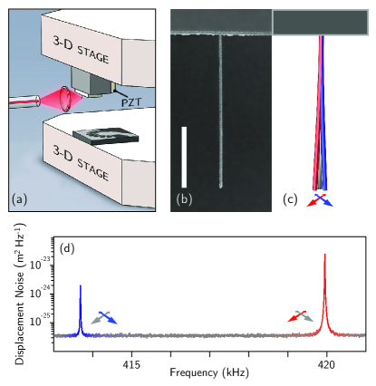
Figure 1: Schematic drawing of the measurement setup. a A fiber-optic interferometer is aligned with a single NW using a piezoelectric positioning stage (top). A second stage (bottom) is used to position and scan the sample surface under the NW. b, A scanning electron micrograph (SEM) of NW1, a typical GaAs/AlGaAs NW. The scale bar represents 10 $\mu$m. c, A schematic diagram showing the two orthogonal fundamental flexural modes of the NW. d The displacement spectral noise density of the fundamental mode doublet measured by fiber-optic interferometry for NW1. We extract $\theta_{0}=15^{\circ}$.

We resolve the two first-order flexural modes with different signal-to-noise ratio, given that the principal axes $\mathbf{\hat{r}}_{1}$ and $\mathbf{\hat{r}}_{2}$ of the modes are rotated by some angle $\theta_{0}$ with respect to the optical detection axis $\mathbf{\hat{x}}$ nichol_displacement_2008 . The total measured displacement is $x(t)=r_{1}(t)\sin\theta_{0}+r_{2}(t)\cos\theta_{0}$, where $r_{1}$ and $r_{2}$ represent the displacement of each flexural mode. The mean square displacement generated by uncorrelated thermal noise is then $\langle x^{2}\rangle=P_{1}+P_{2}$, where $P_{1}=\langle r^{2}_{1}\rangle\sin^{2}\theta_{0}$ and $P_{2}=\langle r^{2}_{2}\rangle\cos^{2}\theta_{0}$ represent the integrated power of each measured resonance in the spectral density. Given that the motional mass $m$ of the two orthogonal flexural modes is the same, using the equipartition theorem, we find the ratio of their mean-square thermal displacements $\langle r_{1}^{2}\rangle/\langle r_{2}^{2}\rangle=f_{2}^{2}/f_{1}^{2}$. Therefore, from the measured thermal peaks in the spectral density, we calculate the angle $\theta_{0}=\arctan\left(\frac{f_{1}}{f_{2}}\sqrt{\frac{P_{1}}{P_{2}}}\right)$ between $\mathbf{\hat{r}}_{1}$ ($\mathbf{\hat{r}}_{2}$) and $\mathbf{\hat{x}}$ ($\mathbf{\hat{y}}$). Furthermore, since $k_{i}=k_{B}T/\langle r_{i}^{2}\rangle$, where $i=1,2$, we obtain the spring constants of each flexural mode, which are typically on the order of 100 mN/m. These parameters yield mechanical dissipations $\Gamma_{i}=k_{i}/(2\pi f_{i}Q_{i})$ and thermally limited force sensitivities $S_{F_{i}}^{1/2}=\sqrt{4k_{B}T\Gamma_{i}}$ around 10 ng/s and 5 aN/$\sqrt{\text{Hz}}$, respectively.

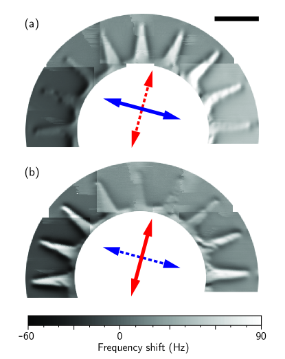
Figure 2: Mode 1 and mode 2 frequency shift images. Left (Right) panel shows $\Delta f_{1}(x,y)$ ($\Delta f_{2}(x,y)$) of NW1, , which has $\theta_{0}=15^{\circ}$, at a distance of 70 nm from a pattern of Au finger gates on a Si substrate. Gray scale is proportional to the respective frequency shifts and the blue (red) arrows show the direction $\mathbf{\hat{r}}_{1}$ ($\mathbf{\hat{r}}_{2}$) of mode 1 (2) as determined by thermal noise measurements far from the surface. The scale bar represents 2 $\mu$m.

III Two-mode scanning probe microscopy

In order to use the NW as a scanning probe, we approach the sample and scan it in a plane below the NW tip. By monitoring the NW’s mechanical properties, i.e. the frequency, dissipation, and orientation of its doublet modes, we image the sample topography via the tip-sample interaction. Such microscopy can be accomplished by measuring the NW thermal displacement spectral density as the sample surface is scanned below it. Although such a measurement provides a full mechanical characterization of the modes, it is time-consuming due to the small displacement. A technique more amenable to fast spatial scans uses the resonant excitation of the doublet modes through two independent phase-locked loops (PLLs) to track both frequencies simultaneously (see Appendix).

Fig. 2 shows the frequency shifts $\Delta f_{1}(x,y)$ and $\Delta f_{2}(x,y)$ of the doublet modes as a sample is scanned below the tip of NW1. The sample consists of nine 5-$\mu$m long and 200-nm thick finger gates of Au on a Si substrate, radially disposed and equally spaced along a semicircle (see Supplementary Information for an SEM of the sample). The finger gates and their tapered shape are intended to provide edges at a variety of different angles, highlighting the directional sensitivity of the orthogonal modes. The measurement in Fig. 2 is performed using the PLL with an oscillation amplitude of 50 nm at a distance of 70 nm from the Au surfaces in “open loop”, i.e. without feedback to maintain a constant distance from the sample. The Au gates are grounded during the measurement.

The frequency shift images clearly delinate the topography of the patterned sample, with each mode showing stronger contrast for features aligned along orthogonal directions. These two directions (identified by noting the direction of the fingers with maximum contrast) agree with the angle $\theta_{0}=15^{\circ}$ measured for NW1 via the thermal noise shown in Fig. 1(d). Edges, i.e. large topographical gradients, pointing perpendicular (parallel) to the mode oscillation direction appear to produce the strongest (weakest) contrast. Tip-sample interactions producing the frequency shifts in non-contact AFM can include electrostatic, van der Waals, or chemical bonding forces depending on the distance. In our case, because of the large spacing, they are dominated by electrostatic forces.

IV Extraction of spatial tip-sample force derivatives

In order to understand the measurements, we describe the motion of the NW tip in each of the two fundamental flexural modes as a driven damped harmonic oscillator:

$$m\ddot{r_{i}}+\Gamma_{i}\dot{r_{i}}+k_{i}r_{i}=F_{th}+F_{i},$$ (1)

where $m$ is the effective mass of the fundamental flexural modes, $F_{th}$ is the Langevin force, $F_{i}$ is the component of the tip-sample force along $\mathbf{\hat{r}}_{i}$, and $i=1,2$. Following the treatment of Gloppe et al. gloppe_bidimensional_2014 and expanding $F_{i}$ for small oscillations around the equilibrium $r_{i}=0$, we have $F_{i}\approx F_{i}(0)+\left.r_{j}\partial F_{i}/\partial r_{j}\right|_{0}$. By replacing this expansion in (5), we find that this tip-sample interaction produces new doublet eigenmodes with modified spring constants $k_{i}^{\prime}$ (see Supplementary Information):

$$\begin{split}k_{1,2}^{\prime}&=\frac{1}{2}\bigg{[}k_{1}+k_{2}-F_{11}-F_{22}\\ &\qquad\pm\sqrt{(k_{1}-k_{2}-F_{11}+F_{22})^{2}+4F_{12}F_{21}}\bigg{]},\\ \end{split}$$ (2)

where we use a shorthand notation for the force derivatives $F_{ij}\equiv\left.\partial F_{i}/\partial r_{j}\right|_{0}$. In addition to inducing frequency shifts, tip-sample force derivatives with non-zero shear components ($F_{ij}\neq 0$ for $i\neq j$) couple the two flexural modes and rotate their oscillation direction along two new basis vectors $\mathbf{\hat{r}}_{i}^{\prime}$ faust_nonadiabatic_2012 . These new modes remain orthogonal for conservative force fields (i.e. $F_{12}=F_{21}$), but lose their orthogonality for non-conservative force fields.

For tip-sample force derivatives that are much smaller than the bare NW spring constant – which is the case here – the modified spring constants $k_{i}^{\prime}\approx k_{i}-F_{ii}$. Therefore, by monitoring the frequency shift between the bare resonances and those modified by the tip-sample interaction $\Delta f_{i}=f_{i}^{\prime}-f_{i}$, we measure:

$$\left.\frac{\partial F_{i}}{\partial r_{i}}\right|_{0}\approx-2k_{i}\left(\frac{\Delta f_{i}}{f_{i}}\right),$$ (3)

Because the oscillation amplitude ($\sim 50$ nm) is small compared to the tip diameter ($\sim 350$ nm), we can ignore variations of the force derivative over the oscillation cycle. Just as in conventional 1D dynamic lateral force microscopy, each $\Delta f_{i}(x,y)$ depends on the derivative $F_{ii}$, i.e. on the force both projected and differentiated along the mode oscillation direction. The NW mode doublet, however, is able to simultaneously measure force derivatives along orthogonal directions.

In the same limit of small derivatives considered for (8), the rotation of the mode axes reveals the shear, or cross derivatives of the force, through,

$$\left.\frac{\partial F_{i}}{\partial r_{j}}\right|_{0}\approx\left|k_{i}-k_{j}\right|\tan\phi_{i},$$ (4)

for $i\neq j$ and where $\phi_{i}=\theta_{i}-\theta_{0}$ is the angle between the mode direction $\mathbf{\hat{r}}_{i}^{\prime}$ in the presence of tip-surface interaction and the bare mode direction $\mathbf{\hat{r}}_{i}$. Therefore by monitoring the doublet mode frequency shifts and oscillation directions, we can completely determine the in-plane tip-sample force derivatives $F_{ij}$.

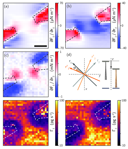
Figure 3: 2D Force derivative and dissipation images. a, b, c, Force derivatives $F_{11}$, $F_{22}$, and $F_{12}=F_{21}$, respectively, extracted from thermal noise data as a function of the $xy$-position of NW2 70 nm over the gated sample. Overlayed dashed lines indicate the edges of the finger gates, as obtained by SEM. d, Schematic picture of the direction of the flexural eigenmodes at two tip-sample distances $z$. The black and gray axes indicate the direction of the unperturbed axes with $\theta_{0}=46^{\circ}$. The eigenmodes rotate through an angle $\phi$ when brought closer to the sample. e, f Dissipation $\Gamma_{i}$ of each mode as a function of the $xy$-position.

V Imaging static in-plane force derivatives and dissipation

A complete measurement of static in-plane force derivatives and dissipations is shown in Fig. 3 for a section of the “finger” sample using a second NW, NW2. $\Delta f_{i}$ and $\Gamma_{i}$ are extracted from fits to the spectral density of the thermal noise measured as the sample was scanned below the NW at a fixed spacing of 70 nm. By assuming a conservative tip-sample interaction ($F_{ij}=F_{ji}$), we determine $\phi=\phi_{1}=\phi_{2}$ from the frequency and integrated power of each mode in the spectral density compared to a similar measurement far from the surface, giving $\theta_{0}=46^{\circ}$. Using these data along with (8) and (9), we produce maps of $F_{ij}(x,y)$ and $\Gamma_{i}(x,y)$. The measurements show strong positive followed by negative $F_{ii}$ for edges perpendicular to the NW mode oscillation $\mathbf{\hat{r}}_{i}$. In non-contact AFM, tip-samples forces are generally attractive and become more so with decreasing tip-sample distance and increased interaction area. As the NW approaches a Au edge perpendicular to $\mathbf{\hat{r}}_{i}$ from a position above the lower Si surface, it will experience an increasingly attractive force, i.e. a positive $F_{ii}$. After the midpoint of the tip crosses this edge, the attractive force starts to drop off, resulting in a negative $F_{ii}$. As expected, measurements show that $F_{ij}$ for $i\neq j$ are peaked around curved edges. Measured tip-sample dissipations $\Gamma_{i}$ are nearly isotropic and appear to reflect the different materials and tip-sample spacings over the Au fingers and the Si substrate. Similar 1D measurements of non-contact friction also show lower values over conducting surfaces like Au compared to insulating surfaces like Si and point to charge fluctuations as the origin for the dissipation stipe_noncontact_2001 ; kuehn_dielectric_2006 .

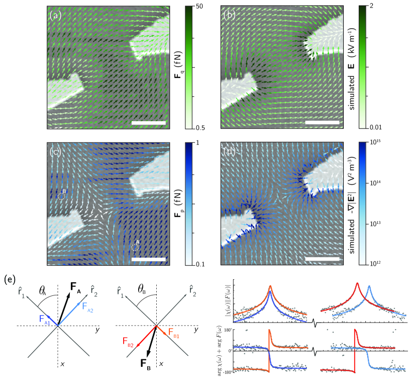
Figure 4: Vector plots of electrostatic force fields. a Vector plot of the force field induced by an electric field on the charged NW. The vector plot is overlayed on top of a SEM image of the sample. b, Vector plot of the simulated electric field $\mathbf{E}(\mathbf{r})$ induced by the biased finger gates. c Vector plot of the force field induced by the electric field on the polarizable NW. The voltage amplitude applied to the gates in a and c is $V=2$ and $20$ mV, respectively, the vertical spacing between NW2 and the Au gates is 70 nm, and $\theta_{0}=46^{\circ}$. d, Vector plot of the simulated values of $-\mathbf{\nabla}|\mathbf{E(\mathbf{r})}|^{2}$ induced by the biased finger gates. e, The diagram shows schematic diagrams of how force vectors are extracted from measurements at the example positions A and B. The amplitude and orientation of the force is extracted from fits to the amplitude and phase response as a function of frequency of the two modes, shown in the corresponding plots.

VI Imaging a dynamic in-plane force field

In-plane force fields can also be mapped with a thermally limited sensitivity of 5 aN/$\sqrt{\text{Hz}}$ by measuring the driven NW response, as shown in Fig. 4. The frequency of the force to be measured must be swept through the NW doublet resonances, while the amplitude and phase of the displacement response is recorded. As an example, we apply a small AC voltage $V\cos(2\pi ft)$ with frequency $f$ producing an oscillating electric field $\mathbf{E}(\mathbf{r},t)$ between opposing finger gates. In scanning the NW and measuring its response, we distinguish between two types of forces. The first shows a linear dependence on the electric field strength and is associated with charge: $\mathbf{F_{q}}=q\mathbf{E}$, where $q$ is the net charge on the NW tip. The second force exhibits a quadratic dependence on the field strength and is associated with the induced dipolar moment of the dialectric NW, i.e. with its polarizability: $\mathbf{F_{p}}=-\mathbf{\nabla}(\alpha|\mathbf{E}|^{2})$, where $\alpha$ is the effective polarizability of the GaAs/AlGaAs NW rieger_frequency_2012 . Due to their linear and quadratic dependence on $\mathbf{E}$, respectively, $\mathbf{F_{q}}$ drives the NW at frequency $f$, while $\mathbf{F_{p}}$ drives it at DC and $2f$. As a result, the two interactions can be spectrally separated.

The magnitude and orientation of the driving force along each doublet mode direction can be extracted from the displacement and phase response of each mode as a function of frequency, as shown schematically in Fig. 4(e). A measurement of the thermal noise spectrum in the absence of the AC drive is used to calibrate the orientation of the mode doublet. By scanning the sample in a plane 70 nm below NW2 and measuring thermal motion and driven response at each point, we construct vectorial maps of the $\mathbf{F}_{q}$ and $\mathbf{F}_{p}$, as shown in Fig. 4(a) and (c) and described in the Appendix. These measured force fields are compared to the $\mathbf{E}$ and $-\mathbf{\nabla}|\mathbf{E}^{2}|$ fields simulated by FEM analysis (COMSOL) using the real gate geometries in Figs. 4(b) and (d). Dividing the measured force fields by the corresponding simulations, we determine the net charge on the tip of NW2 to be $q=30\pm 10$ $e$, where $e$ is the fundamental charge, and the effective polarizability $\alpha=10^{-29}$ $\text{C}/(\text{V}\cdot\text{m})$, which is roughly consistent with the size and dielectric constant of the NW. The ability to vectorially map electric fields on the nanometer-scale extends the capability of conventional AFM to image charges stern_deposition_1988 ; schonenberger_observation_1990 and contact potential differences nonnenmacher_kelvin_1991 and has applications in localizing electronic defects on or near surfaces, e.g. in microelectronic failure analysis.

VII Conclusion and Outlook

Our measurements demonstrate the potential of NWs as sensitive scanning vectorial force sensors. By monitoring two orthogonal flexural modes while scanning over a sample surface, we map forces and force derivatives in 2D. While we demonstrate the technique on electrostatic tip-sample interactions, it is generally applicable and could, for instance, be used to measure magnetic forces with proper functionalization of the NW tip or even in liquid sanii_high_2010 for the study of batteries, water splitting, or fuel cells. Note that in the presented data, the 350-nm diameter of the NW tip strongly limits the spatial resolution of the microscopy. Nevertheless, the same technique could be applied to NWs grown or processed to have sharp tips, presenting the possibility of atomic-scale or even sub-atomic-scale force microscopy with directional sensitivity, a feat already achieved in 1D kawai_ultrasensitive_2010 . Therefore, one could imagine the use of vectorial NW-based AFM of tip-sample forces and non-contact friction to reveal, for example, the anisotropy of atomic bonding forces.

VIII Acknowledgements

Appendix A Appendix A: Nanowire growth and processing

MBE synthesis of the GaAs/AlGaAs NWs starts on a Si substrate with the growth of a 290-nm thick GaAs NW core along $[1\,\bar{1}\,1]$ by the Ga-assisted method detailed in Uccelli et al. uccelli_three-dimensional_2011 and Russo-Averchi et al russo-averchi_suppression_2012 . Axial growth is stopped once the NWs are about 25-$\mu$m long by temporarily blocking the Ga flux and reducing the substrate temperature from 630 down to $465^{\circ}$C. Finally, a 50-nm thick Al_0.51Ga_0.49As shell capped by a 5-nm GaAs layer is grown heigoldt_long_2009 . For optimal inferometric detection of the NWs, we focus on NWs within 40 $\mu$m from the substrate edge. To avoid measuring multiple NWs or having interference between NWs, we reduce the NW density in the area of interest using a micromanipulator under an optical microscope.

Appendix B Appendix B: Nanowire positioning and displacement detection

The measurement chamber includes two stacks of piezoelectric positioners (Attocube AG) to independently control the 3D position of the NW cantilevers and the sample of interest with respect to the fixed detection optics. The top stack is used to align a single NW within the focus of a fiber-coupled optical interferometer used to detect its mechanical motion rugar_improved_1989 . Once the NW and interferometer are aligned, the bottom stack is used to approach and scan the sample of interest with respect to the NW cantilever. Light from a laser diode with wavelength of 635 nm is sent through one arm of a 50:50 fiber-optic coupler and focused by a pair of lenses to a 1-$\mu$m spot. The incident power of $\sim 5\mu$W does not significantly heat the NW as confirmed by measurements of laser power dependence and mechanical thermal motion. Despite the sub-$\mu$m diameter of the NW, it reflects a portion of the light back into the fiber, which interferes with light reflected by the fiber’s cleaved end. The resulting low-finesse Fabry-Perot interferometer acts as a sensitive sensor of the NW displacement, where the interference intensity is measured by a fast photoreceiver with an effective 3 dB bandwidth of 800 kHz.

Appendix C Appendix C: Measurement protocols

Measurements of NW thermal motion used for Figs. 1, 3 and 4 are made using a analog-to-digital converter (National Instruments). Fits based on the thermally driven damped harmonic oscillator of (5) are used to extract $\theta_{0}$, $f_{i}$, $\Gamma_{i}$, $m$, and $\phi_{i}$. Faster measurements, as in Fig. 2, are performed by resonantly exciting both flexural modes using the piezoelectric transducer. Due to the high $Q_{i}$ and large $\delta$ of the resonances, it is possible to monitor and control both modes simultaneously. As in standard AFM, we use a lock-in amplifier (Zurich Instruments UHFLI) to resonantly drive each mode and demodulate the resulting optical signal measured by the photoreceiver. For each mode, its shift in resonant frequency $\Delta f_{i}$ is tracked by a PLL, while proportional-integral control of the excitation voltage maintains a constant oscillation amplitude. Measurements of the NW amplitude and phase response to a time-varying gate voltage applied to the the sample, as shown in Fig. 4, are made using the same lock-in. Fits to the amplitude and phase response of each mode as a function of frequency are based on the mechanical susceptibility $\chi_{i}(\omega)=1/(k_{i}-m\omega^{2}+i\Gamma_{i}\omega)$ of a damped harmonic oscillator, where $\omega=2\pi f$. The oscillation amplitude $|\chi_{i}(\omega)||F_{i}(\omega)|$ excited for mode $i$ gives the magnitude of the driving force $F_{i}$ along $\mathbf{\hat{r}}_{i}$. The phase $\arg F_{i}(\omega)$ gives the orientation of $F_{i}$ along either positive or negative $\mathbf{\hat{r}}_{i}$.

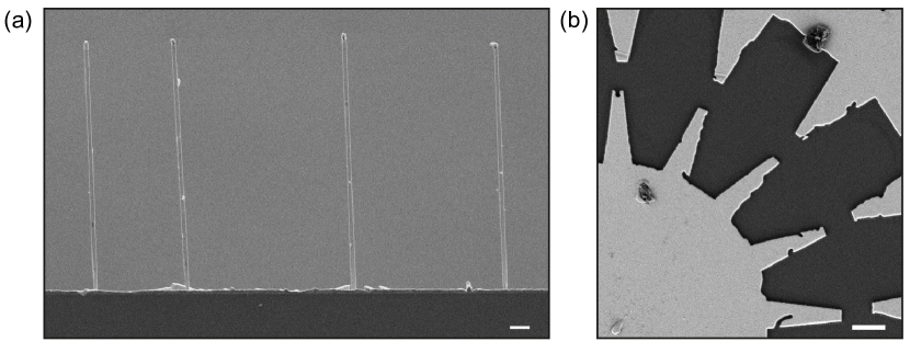
Figure 5: Supplementary. a, Zoomed out SEM image of the edge of the NW sample, showing several similar NWs. b Zoomed out SEM image of the finger gate sample. The scalebar in both figures corresponds to 2$\mu$m.

Appendix D Supplementary Information: Nanowire motion in presence of tip-sample force

We describe the motion of the NW tip in each of the two fundamental flexural modes as a driven damped harmonic oscillator:

$$m\ddot{r_{i}}+\Gamma_{i}\dot{r_{i}}+k_{i}r_{i}=F_{th}+F_{i},$$ (5)

where $m$ is the effective mass of the fundamental flexural modes, $F_{th}$ is the Langevin force, $F_{i}$ is the component of the tip-sample force along the mode oscillation direction $\mathbf{\hat{r}}_{i}$, and $i=1,2$. Following the treatment of Gloppe et al. gloppe_bidimensional_2014 and expanding $F_{i}$ for small oscillations around the equilibrium $r_{i}=0$, we have,

$$F_{i}\approx F_{i}(0)+\left.r_{j}\frac{\partial F_{i}}{\partial r_{j}}\right|_{0}.$$ (6)

By replacing this expansion in (5), we have,

$$m\ddot{r_{i}}+\Gamma_{i}\dot{r_{i}}+k_{i}r_{i}=F_{th}+F_{i}(0)+F_{ij}r_{j},$$ (7)

where we use a shorthand notation for the force derivatives $F_{ij}\equiv\left.\frac{\partial F_{i}}{\partial r_{j}}\right|_{0}$. As (7) makes clear, the derivatives of the tip-sample force modify and couple the NW’s two unperturbed flexural modes. We now rewrite this equation in vectorial form as,

$$m\ddot{\mathbf{r}}+\bar{\Gamma}\cdot\dot{\mathbf{r}}+\bar{K}\cdot\mathbf{r}=F_{th}+\mathbf{F}_{0},$$ (8)

where $\mathbf{r}=\left(\begin{smallmatrix}r_{1}\\ r_{2}\end{smallmatrix}\right)$ and the equilibrium tip-sample force $\mathbf{F}_{0}=\mathbf{F}(\mathbf{r}=0)$. The dissipation and spring constant matrices are defined by:

$$\bar{\Gamma}\equiv\begin{pmatrix}\Gamma_{1}&0\\ 0&\Gamma_{2}\end{pmatrix},$$ (9)

$$\bar{K}\equiv\begin{pmatrix}k_{1}-F_{11}&-F_{21}\\ -F_{12}&k_{2}-F_{22}\end{pmatrix},$$ (10)

where the role of the shear cross-derivatives, i.e. $F_{ij}$ for $i\neq j$, in coupling the unperturbed NW modes is clear faust_nonadiabatic_2012 . In the presence of weak tip-surface interactions, as those studied here, the dissipation rates of the NW modes are neglibly small compared to their unperturbed resonant frequencies, i.e. $\frac{\Gamma}{2m}\ll\sqrt{\frac{k}{m}}$. In this limit, the NW mode frequencies and oscillation directions are determined by $\bar{K}$. Therefore, by diagonalizing $\bar{K}$, we find a new pair of uncoupled flexural modes. The corresponding spring constants and mode directions have been modified from the unperturbed state by the spatial tip-sample force derivatives $F_{ij}$:

$$k_{1}^{\prime} =\frac{1}{2}\bigg{[}k_{1}+k_{2}-F_{11}-F_{22}$$

$$\qquad+\sqrt{(k_{1}-k_{2}-F_{11}+F_{22})^{2}+4F_{12}F_{21}}\bigg{]},$$ (11)

$$\mathbf{\hat{r}}_{1}^{\prime} =\frac{1}{\sqrt{(k_{2}-F_{22}-k_{1}^{\prime})^{2}+F_{12}^{2}}}\begin{pmatrix}k_{2}-F_{22}-k_{1}^{\prime}\\ F_{12}\end{pmatrix};$$ (12)

$$k_{2}^{\prime} =\frac{1}{2}\bigg{[}k_{1}+k_{2}-F_{11}-F_{22}$$

$$\qquad-\sqrt{(k_{1}-k_{2}-F_{11}+F_{22})^{2}+4F_{12}F_{21}}\bigg{]},$$ (13)

$$\mathbf{\hat{r}}_{2}^{\prime} =\frac{1}{\sqrt{(k_{1}-F_{11}-k_{2}^{\prime})^{2}+F_{21}^{2}}}\begin{pmatrix}F_{21}\\ k_{1}-F_{11}-k_{2}^{\prime}\end{pmatrix}.$$ (14)

These new modes remain orthogonal ($\mathbf{\hat{r}}_{1}^{\prime}\cdot\mathbf{\hat{r}}_{2}^{\prime}=0$) for conservative force fields ($\nabla\times\mathbf{F}=0$, i.e. $F_{12}-F_{21}=0$), but lose their orthogonality for non-conservative force fields.

For tip-sample force derivatives that are much smaller than the bare NW spring constants – which is the case here – the modified spring constants and the modified mode directions in (11) - (14) can be approximated to first order in the derivatives:

$$k_{1}^{\prime}\approx k_{1}-F_{11},$$ (15)

$$\mathbf{\hat{r}}_{1}^{\prime}\approx\frac{1}{\sqrt{(k_{1}-k_{2})^{2}+F_{12}^{2}}}\begin{pmatrix}k_{1}-k_{2}\\ -F_{12}\end{pmatrix};$$ (16)

$$k_{2}^{\prime}\approx k_{2}-F_{22},$$ (17)

$$\mathbf{\hat{r}}_{2}^{\prime}\approx\frac{1}{\sqrt{(k_{1}-k_{2})^{2}+F_{21}^{2}}}\begin{pmatrix}F_{21}\\ k_{1}-k_{2}\end{pmatrix}.$$ (18)

In the limit of small dissipation discussed previously, the unperturbed resonance frequencies of the flexural modes are given by $f_{i}=\frac{1}{2\pi}\sqrt{\frac{k_{i}}{m}}$. Similarly, the modified resonance frequencies are given by $f_{i}^{\prime}=\frac{1}{2\pi}\sqrt{\frac{k_{i}^{\prime}}{m}}$. For small tip-sample force derivatives, we apply (15) and (17) and arrive at $f_{i}^{\prime}\approx\frac{1}{2\pi}\sqrt{\frac{k_{i}-F_{ii}}{m}}$. Expanding to first order in $F_{ii}$, we find $f_{i}^{\prime}\approx f_{i}-\frac{f_{i}}{2k_{i}}F_{ii}$. Solving in terms of the frequency shift induced by the tip-sample interaction, we have:

$$\Delta f_{i}=f_{i}^{\prime}-f_{i}\approx-\frac{f_{i}}{2k_{i}}F_{ii}.$$ (19)

We can now write a relation for $F_{ii}=\partial F_{i}/\partial r_{i}$ in terms of the measured frequency shift induced by the tip-sample interaction and properties of the unperturbed NW modes:

$$\frac{\partial F_{i}}{\partial r_{i}}\approx-2k_{i}\left(\frac{\Delta f_{i}}{f_{i}}\right).$$ (20)

Using (16) and (18), we can also write an expression involving the angle $\phi_{i}$ between the bare mode direction $\mathbf{\hat{r}}_{i}$ and the corresponding modified mode direction $\mathbf{\hat{r}}_{i}^{\prime}$:

$$\tan{\phi_{i}}\approx\frac{F_{ij}}{\left|k_{i}-k_{j}\right|}.$$ (21)

This equation then allows us to solve for $F_{ij}=\partial F_{i}/\partial r_{j}$ for $i\neq j$ in terms of the measured angles $\phi_{i}$ and the unperturbed spring constants:

$$\frac{\partial F_{i}}{\partial F_{j}}\approx|k_{i}-k_{j}|\tan{\phi_{i}}.$$ (22)

In this way, we are able to measure all spatial tip-sample force derivatives in the small interaction limit (i.e. all derivatives much smaller than the unperturbed spring constants).

References

- (1) Binnig, G., Quate, C. F. & Gerber, C. Atomic Force Microscope. Phys. Rev. Lett. 56, 930–933 (1986). URL http://link.aps.org/doi/10.1103/PhysRevLett.56.930.
- (2) Giessibl, F. J. Advances in atomic force microscopy. Rev. Mod. Phys. 75, 949–983 (2003). URL http://link.aps.org/doi/10.1103/RevModPhys.75.949.
- (3) Giessibl, F. J. Atomic Resolution of the Silicon (111)-(7x7) Surface by Atomic Force Microscopy. Science 267, 68–71 (1995). URL http://www.sciencemag.org/content/267/5194/68.
- (4) Giessibl, F. J., Hembacher, S., Bielefeldt, H. & Mannhart, J. Subatomic Features on the Silicon (111)-(77) Surface Observed by Atomic Force Microscopy. Science 289, 422–425 (2000). URL http://www.sciencemag.org/content/289/5478/422.
- (5) Poggio, M. Sensing from the bottom up. Nat. Nanotechnol. 8, 482–483 (2013). WOS:000321248700007.
- (6) Sazonova, V. et al. A tunable carbon nanotube electromechanical oscillator. Nature 431, 284–287 (2004). URL http://www.nature.com/nature/journal/v431/n7006/abs/nature02905.html.
- (7) Bunch, J. S. et al. Electromechanical Resonators from Graphene Sheets. Science 315, 490–493 (2007). URL http://www.sciencemag.org/content/315/5811/490.
- (8) Perisanu, S. et al. High Q factor for mechanical resonances of batch-fabricated SiC nanowires. Applied Physics Letters 90, 043113 (2007). URL http://scitation.aip.org/content/aip/journal/apl/90/4/10.1063/1.2432257.
- (9) Feng, X. L., He, R., Yang, P. & Roukes, M. L. Very High Frequency Silicon Nanowire Electromechanical Resonators. Nano Lett. 7, 1953–1959 (2007). URL http://dx.doi.org/10.1021/nl0706695.
- (10) Nichol, J. M., Hemesath, E. R., Lauhon, L. J. & Budakian, R. Displacement detection of silicon nanowires by polarization-enhanced fiber-optic interferometry. Applied Physics Letters 93, 193110 (2008). URL http://scitation.aip.org/content/aip/journal/apl/93/19/10.1063/1.3025305.
- (11) Li, M. et al. Bottom-up assembly of large-area nanowire resonator arrays. Nat Nano 3, 88–92 (2008). URL http://www.nature.com/nnano/journal/v3/n2/full/nnano.2008.26.html.
- (12) Belov, M. et al. Mechanical resonance of clamped silicon nanowires measured by optical interferometry. Journal of Applied Physics 103, 074304 (2008). URL http://scitation.aip.org/content/aip/journal/jap/103/7/10.1063/1.2891002.
- (13) Gil-Santos, E. et al. Nanomechanical mass sensing and stiffness spectrometry based on two-dimensional vibrations of resonant nanowires. Nat Nano 5, 641–645 (2010). URL http://www.nature.com/nnano/journal/v5/n9/full/nnano.2010.151.html.
- (14) Chaste, J. et al. A nanomechanical mass sensor with yoctogram resolution. Nat Nano 7, 301–304 (2012). URL http://www.nature.com/nnano/journal/v7/n5/full/nnano.2012.42.html?WT.ecid=NNANO-201205.
- (15) Moser, J. et al. Ultrasensitive force detection with a nanotube mechanical resonator. Nat Nano 8, 493–496 (2013). URL http://www.nature.com/nnano/journal/v8/n7/full/nnano.2013.97.html.
- (16) Gysin, U., Rast, S., Kisiel, M., Werle, C. & Meyer, E. Low temperature ultrahigh vacuum noncontact atomic force microscope in the pendulum geometry. Review of Scientific Instruments 82, 023705 (2011). URL http://scitation.aip.org/content/aip/journal/rsi/82/2/10.1063/1.3551603.
- (17) Nichol, J. M., Hemesath, E. R., Lauhon, L. J. & Budakian, R. Nanomechanical detection of nuclear magnetic resonance using a silicon nanowire oscillator. Phys. Rev. B 85, 054414 (2012). URL http://link.aps.org/doi/10.1103/PhysRevB.85.054414.
- (18) Nichol, J. M., Naibert, T. R., Hemesath, E. R., Lauhon, L. J. & Budakian, R. Nanoscale Fourier-Transform Magnetic Resonance Imaging. Phys. Rev. X 3, 031016 (2013). URL http://link.aps.org/doi/10.1103/PhysRevX.3.031016.
- (19) Nonnenmacher, M., OBoyle, M. P. & Wickramasinghe, H. K. Kelvin probe force microscopy. Applied Physics Letters 58, 2921–2923 (1991). URL http://scitation.aip.org/content/aip/journal/apl/58/25/10.1063/1.105227.
- (20) Stipe, B. C., Mamin, H. J., Stowe, T. D., Kenny, T. W. & Rugar, D. Noncontact Friction and Force Fluctuations between Closely Spaced Bodies. Phys. Rev. Lett. 87, 096801 (2001). URL http://link.aps.org/doi/10.1103/PhysRevLett.87.096801.
- (21) Gloppe, A. et al. Bidimensional nano-optomechanics and topological backaction in a non-conservative radiation force field. Nature Nanotechnology 9, 920–926 (2014). URL http://www.nature.com/nnano/journal/v9/n11/full/nnano.2014.189.html.
- (22) Pfeiffer, O., Bennewitz, R., Baratoff, A., Meyer, E. & Grütter, P. Lateral-force measurements in dynamic force microscopy. Phys. Rev. B 65, 161403 (2002). URL http://link.aps.org/doi/10.1103/PhysRevB.65.161403.
- (23) Giessibl, F. J., Herz, M. & Mannhart, J. Friction traced to the single atom. PNAS 99, 12006–12010 (2002). URL http://www.pnas.org/content/99/19/12006.
- (24) Kawai, S., Kitamura, S.-i., Kobayashi, D. & Kawakatsu, H. Dynamic lateral force microscopy with true atomic resolution. Applied Physics Letters 87, 173105 (2005). URL http://scitation.aip.org/content/aip/journal/apl/87/17/10.1063/1.2112203.
- (25) Kawai, S., Sasaki, N. & Kawakatsu, H. Direct mapping of the lateral force gradient on $\text{Si}(111)\text{-}7\ifmmode\times\else\texttimes\fi{}7$. Phys. Rev. B 79, 195412 (2009). URL http://link.aps.org/doi/10.1103/PhysRevB.79.195412.
- (26) Kawai, S. et al. Ultrasensitive detection of lateral atomic-scale interactions on graphite (0001) via bimodal dynamic force measurements. Phys. Rev. B 81, 085420 (2010). URL http://link.aps.org/doi/10.1103/PhysRevB.81.085420.
- (27) Cadeddu, D. et al. Time-Resolved Nonlinear Coupling between Orthogonal Flexural Modes of a Pristine GaAs Nanowire. Nano Lett. 16, 926–931 (2016). URL http://dx.doi.org/10.1021/acs.nanolett.5b03822.
- (28) Faust, T. et al. Nonadiabatic Dynamics of Two Strongly Coupled Nanomechanical Resonator Modes. Phys. Rev. Lett. 109, 037205 (2012). URL http://link.aps.org/doi/10.1103/PhysRevLett.109.037205.
- (29) Kuehn, S., Loring, R. F. & Marohn, J. A. Dielectric Fluctuations and the Origins of Noncontact Friction. Phys. Rev. Lett. 96, 156103 (2006). URL http://link.aps.org/doi/10.1103/PhysRevLett.96.156103.
- (30) Rieger, J., Faust, T., Seitner, M. J., Kotthaus, J. P. & Weig, E. M. Frequency and Q factor control of nanomechanical resonators. Applied Physics Letters 101, 103110 (2012). URL http://scitation.aip.org/content/aip/journal/apl/101/10/10.1063/1.4751351.
- (31) Stern, J. E., Terris, B. D., Mamin, H. J. & Rugar, D. Deposition and imaging of localized charge on insulator surfaces using a force microscope. Applied Physics Letters 53, 2717–2719 (1988). URL http://scitation.aip.org/content/aip/journal/apl/53/26/10.1063/1.100162.
- (32) Schönenberger, C. & Alvarado, S. F. Observation of single charge carriers by force microscopy. Phys. Rev. Lett. 65, 3162–3164 (1990). URL http://link.aps.org/doi/10.1103/PhysRevLett.65.3162.
- (33) Sanii, B. & Ashby, P. D. High Sensitivity Deflection Detection of Nanowires. Phys. Rev. Lett. 104, 147203 (2010). URL http://link.aps.org/doi/10.1103/PhysRevLett.104.147203.
- (34) Uccelli, E. et al. Three-Dimensional Multiple-Order Twinning of Self-Catalyzed GaAs Nanowires on Si Substrates. Nano Lett. 11, 3827–3832 (2011). URL http://dx.doi.org/10.1021/nl201902w.
- (35) Russo-Averchi, E. et al. Suppression of three dimensional twinning for a 100% yield of vertical GaAs nanowires on silicon. Nanoscale 4, 1486–1490 (2012). URL http://pubs.rsc.org/en/content/articlelanding/2012/nr/c2nr11799a.
- (36) Heigoldt, M. et al. Long range epitaxial growth of prismatic heterostructures on the facets of catalyst-free GaAs nanowires. J. Mater. Chem. 19, 840–848 (2009). URL http://pubs.rsc.org/en/content/articlelanding/2009/jm/b816585h.
- (37) Rugar, D., Mamin, H. J. & Guethner, P. Improved fiber-optic interferometer for atomic force microscopy. Applied Physics Letters 55, 2588–2590 (1989). URL http://scitation.aip.org/content/aip/journal/apl/55/25/10.1063/1.101987.