On the cusp anomalous dimension in the
ladder limit of $\mathcal{N}=4$ SYM

Abstract

We analyze the cusp anomalous dimension in the (leading) ladder limit of $\mathcal{N}=4$ SYM and present new results for its higher-order perturbative expansion. We study two different limits with respect to the cusp angle $\phi$. The first is the light-like regime where $x=e^{i\,\phi}\to 0$. This limit is characterised by a non-trivial expansion of the cusp anomaly as a sum of powers of $\log x$, where the maximum exponent increases with the loop order. The coefficients of this expansion have remarkable transcendentality features and can be expressed by products of single zeta values. We show that the whole logarithmic expansion is fully captured by a solvable Woods-Saxon like one-dimensional potential. From the exact solution, we extract generating functions for the cusp anomaly as well as for the various specific transcendental structures appearing therein. The second limit that we discuss is the regime of small cusp angle. In this somewhat simpler case, we show how to organise the quantum mechanical perturbation theory in a novel efficient way by means of a suitable all-order Ansatz for the ground state of the associated Schrödinger problem. Our perturbative setup allows to systematically derive higher-order perturbative corrections in powers of the cusp angle as explicit non-perturbative functions of the effective coupling. This series approximation is compared with the numerical solution of the Schrödinger equation to show that we can achieve very good accuracy over the whole range of coupling and cusp angle. Our results have been obtained by relatively simple techniques. Nevertheless, they provide several non-trivial tests useful to check the application of Quantum Spectral Curve methods to the ladder approximation at non zero $\phi$, in the two limits we studied.

1 Introduction

The study of cusped Wilson loops $W$ was initiated by Polyakov in Polyakov:1980ca while attempting to view gauge fields as chiral fields on a loop space. Gauge interactions are interpreted in terms of the propagation of infinitely thin rings formed by the lines of color-electric flux. The analysis of the quantum properties of $W$ led to the introduction of the cusp anomalous dimension $\Gamma_{\text{cusp}}(\phi)$ depending on the Euclidean cusp angle $\phi$ and appearing in the relation

$$\langle W\rangle\sim e^{-\Gamma_{\text{cusp}}(\phi)\,\log\frac{\Lambda_{\text{UV}}}{\Lambda_{\text{IR}}}},$$ (1)

where $\Lambda_{\text{UV, IR}}$ are ultraviolet and infrared energy cutoffs. In QCD, the cusp anomalous dimension was first computed at two loops in Korchemsky:1987wg ; Kidonakis:2009ev and has been recently extended to three loops in Grozin:2014hna ; Grozin:2015kna , see also Kidonakis:2016voy . In supersymmetric theories, it is possible to introduce a locally supersymmetric Wilson loop that couples to scalars in addition to gluons. In $\mathcal{N}=4$ SYM, the cusp anomalous dimension has been computed at two loops in Makeenko:2006ds ; Drukker:2011za , at three loops in Correa:2012nk , and at four loops in Henn:2013wfa .

The free parameter $\phi$ can be tuned to discuss several interesting physical regimes. At small cusp angle, we are doing perturbation around the straight line configuration, $\phi=0$, that is half BPS and has no quantum corrections. The first non-trivial term in the small angle expansion is $\Gamma_{\text{cusp}}(\phi)=-B(\lambda)\,\phi^{2}+\mathcal{O}(\phi^{4})$ where $B(\lambda)$ is the so-called Bremstrahlung function (depending on the planar ’t Hooft coupling $\lambda$) which is fully known Correa:2012at ; Fiol:2012sg . From $\Gamma_{\text{cusp}}(\phi)$, we can extract the potential for a quark anti-quark pair living on a 3-sphere and separated by the angle $\delta=\pi-\phi$. In the limit $\delta\to 0$, the flat space potential is recovered. Finally, one can analytically continue in the cusp angle and consider the limit $\varphi=i\,\phi\to\infty$ where it turns out that $\Gamma_{\text{cusp}}\sim\varphi\,\Gamma_{\text{cusp}}^{\infty}$. The coefficients $\Gamma_{\text{cusp}}^{\infty}$ is the anomalous dimension of a null Wilson loop and is related to the high-spin behaviour of anomalous dimensions of composite operators Korchemsky:1988si ; Korchemsky:1992xv ; Alday:2007mf , governed by the celebrated BES exact integral equation derived in Beisert:2006ez by integrability methods in $\mathcal{N}=4$ SYM.

A quite important feature of the $\mathcal{N}=4$ SYM case is that it is possible to introduce an additional angle in the definition of the Wilson loop Drukker:1999zq . The locally supersymmetric Wilson loop contains a coupling $\int dt\,\Phi\cdot n\,|\dot{x}(t)|$, where $\Phi$ is the vector of the 6 scalars of $\mathcal{N}=4$ SYM and $x(t)$ is the piece-wise straight quark (anti-quark) trajectory Maldacena:1998im . The unit vector $n\in S^{5}$ is constant apart from a discontinuous turn at the cusp by the angle $\theta$. A crucial remark made in Correa:2012nk is that the extra parameter $\theta$ may be used to study the scaling limit

$$i\,\theta\to\infty,\qquad\widehat{\lambda}=\tfrac{1}{4}\,\lambda\,e^{i\,\theta}\quad\text{fixed}.$$ (2)

The limit (2) is interesting because it selects ladder diagrams and, remarkably, the cusp anomalous dimension may be identified with the ground state energy of a 1d Schrödinger equation. In standard notation, it is a function $\Gamma^{\text{lad}}(\kappa,\phi)=-\Omega(\kappa,\phi)$ where $\kappa=\widehat{\lambda}/\pi^{2}$ and $\Omega>0$ is (essentially) the ground state energy of the Schrödinger problem

$$\begin{split}&\bigg{(}-\frac{d^{2}}{dw^{2}}+V(w,\phi)\bigg{)}\,\psi(w)=-\frac{\Omega^{2}(\kappa,\phi)}{4}\,\psi(w),\qquad w\in\mathbb{R},\\ &V(w,\phi)=-\frac{\kappa}{8}\,\frac{1}{\cosh w+\cos\phi}.\end{split}$$ (3)

Despite its simplicity, the ladder approximation is quite interesting and various remarkable feature of the function $\Gamma^{\rm lad}(\kappa,\phi)$ have been investigated at generic $\phi$ in Correa:2012nk ; Henn:2012qz . In this paper, we reconsider its perturbative expansion in two special limits where we are able to provide new exact results.

Light-like limit $x\to 0$, where $x=e^{i\,\phi}$.

As remarked in Henn:2012qz , the limit $x\to 0$ is interesting because it connects the velocity-dependent cusp anomalous dimension with the light-like cusp anomalous dimension which corresponds to the light-like limit of the edges of the Wilson loop. From the six loop analysis of Henn:2012qz , it is possible to identify the following remarkable structure

$$\begin{split}\Gamma^{\rm lad}&=\sum_{n=0}^{\infty}\bigg{[}b^{(n)}(x)\,x^{n}+\mathcal{O}(x^{n+1})\bigg{]}\,(\kappa/4)^{n},\qquad b^{(n)}(x)=\sum_{k=1}^{2n}b^{(n)}_{k}\,\log^{2n-k}x,\end{split}$$ (4)

where $b^{(n)}_{1}$ is rational, $b^{(n)}_{2}=0$, $b^{(n)}_{3}$ is a rational multiple of $\zeta(2)$, $b^{(n)}_{4}$ is a rational multiple of $\zeta(3)$, $b^{(n)}_{5}$ is a rational multiple of $\zeta(4)$, and all next coefficients $b^{(n)}_{k}$ are linear combinations of products of simple $\zeta$ values with transcendentality degree $\text{d}=k-1$. The degree d gets a contribution equal to $n$ from $\zeta_{n}$ (for even $n$ the involved transcendental constant is $\pi^{2n}$) and is additive with respect to multiplication $\text{d}(AB)=\text{d}(A)+\text{d}(B)$. The expansion in (4) has been determined at six loops by the algorithm discussed in Henn:2012qz involving harmonic polylogarithms and their small $x$ expansions. In that approach, it is non trivial to explore the above properties of the coefficients in (4). Here, we study the $x\to 0$ limit of the ladder Schrödinger potential by a different analytical approach. In particular, we identify a reduced Schrödinger equation that captures all the logarithmic terms in (4). It is a 1d version of the three-dimensional Woods-Saxon potential. Its ground state is solvable and from its explicit expression we derive several useful generating functions for the the coefficients $b^{(n)}_{k}$. They are exact in $\kappa$ and can be used to systematically obtain long expansions at higher-loop order.

Small angle $\phi$

For $\phi=0$, the ladder approximation reduces to a Schrödinger equation with solvable Pöschl-Teller potential, see (3). Perturbation theory in $\phi$ is analytic and takes the form

$$\Gamma^{\rm lad}=\sum_{n=0}^{\infty}c_{n}(\kappa)\,\phi^{2\,n},\qquad\kappa=\frac{\widehat{\lambda}}{\pi^{2}}.$$ (5)

In Correa:2012nk , first order Rayleigh-Schrödinger perturbation theory has been applied to provide the results

$$c_{0}(\kappa)=\frac{1-\sqrt{1+\kappa}}{2},\qquad c_{1}(\kappa)=-\frac{\kappa}{16}\,\frac{1+\sqrt{1+\kappa}}{1+\kappa+2\,\sqrt{1+\kappa}}.$$ (6)

The coefficients in the expansion (6) are interesting because they are non-perturbative in the effective ’t Hooft coupling $\widehat{\lambda}=\pi^{2}\,\kappa$. We show that it is possible to systematically improve (6) by implementing a perturbation method originally proposed in dalgarno1956perturbation that typically works in the case of polynomial perturbations. This method has the advantage of bypassing the machinery of the Rayleigh-Schrödinger approach. The resulting algorithm is applied to obtain the coefficient functions $c_{n}(\kappa)$ in closed form for very high $n$. The associated long series expansion is successfully compared with the numerical solution of the Schrödinger problem in the whole range of physical parameters $\kappa,\phi$.

The plan of the paper is the following. In Sec. (2) we study the light-like limit and provide a master equation that permits to easily extract the whole logarithmic expansion in (4) at any loop order. In Sec. (2.1), we further manipulate the master equation showing how to determine a compact generating function for the various transcendentality structures appearing in (4). In Sec. (3), we treat the small $\phi$ perturbative expansion of the cusp anomalous dimension. The higher order results are checked at large $\kappa$ in Sec. (3.1). In Sec. (3.2), we show that our expansions can be used to provide the correct cusp anomaly at all $\kappa$ and $\phi$ with great accuracy. Various appendices collect long results and related discussions.

2 The light-like limit $x\to 0$

As we discussed in the introduction, the first limit we want to treat is $x=e^{i\phi}\to 0$. To explain what we are going to compute, it is convenient to recall the results of Henn:2012qz providing the weak-coupling expansion (4) at 6-loops. We give it in terms of the coefficients $\Omega_{n}(x)$ appearing in, see their Eq. (3.40),

$$\Gamma^{\text{lad}}=-\sum_{n=1}^{\infty}\bigg{(}\frac{1}{4}\,\frac{\kappa\,x}{1-x^{2}}\bigg{)}^{n}\Omega_{n}(x).$$ (7)

When $x\to 0$, the coefficient functions $\Omega_{n}(x)$ have the structure outlined in (4). Writing only the first four non vanishing leading terms, the six loop results obtained in Henn:2012qz are

$$\Omega_{1}(x) =-2\,\log x,$$

$$\Omega_{2}(x) =\frac{4}{3}\,\log^{3}x+4\,\zeta_{2}\,\log x+4\,\zeta_{3}+\mathcal{O}(x),$$

$$\Omega_{3}(x) =-\frac{8}{5}\,\log^{5}x-\frac{32}{3}\,\zeta_{2}\,\log^{3}x-8\,\zeta_{3}\,\log^{2}x-24\,\zeta_{4}\,\log x+\mathcal{O}(1),$$

$$\Omega_{4}(x) =\frac{736}{315}\,\log^{7}x+\frac{368}{15}\,\zeta_{2}\,\log^{5}x+16\,\zeta_{3}\,\log^{4}x+152\,\zeta_{4}\,\log^{3}x+\mathcal{O}(\log^{2}x),$$ (8)

$$\Omega_{5}(x) =-\frac{2144}{567}\,\log^{9}x-\frac{17152}{315}\,\zeta_{2}\,\log^{7}x-\frac{1472}{45}\,\zeta_{3}\,\log^{6}x-\frac{2896}{5}\,\zeta_{4}\,\log^{5}x+\mathcal{O}(\log^{4}x),$$

$$\Omega_{6}(x) =\frac{339008}{51975}\,\log^{11}x+\frac{339008}{2835}\,\zeta_{2}\,\log^{9}x+\frac{4288}{63}\,\zeta_{3}\,\log^{8}x+\frac{12800}{7}\,\zeta_{4}\,\log^{7}x+\mathcal{O}(\log^{6}x).$$

The omitted terms have a uniform transcendentality as discussed in the introduction. They can be found in Henn:2012qz up to 6-loops. Just to give an example, the complete expression of $\Omega_{6}$ is

$$\Omega_{6}(x)\,=\,\frac{339008}{51975}\,\log^{11}x+\frac{339008}{2835}\,\zeta_{2}\,\log^{9}x+\frac{4288}{63}\,\zeta_{3}\,\log^{8}x+\frac{1280\,\pi^{4}}{63}\,\log^{7}x$$

$$\quad+\bigg{(}\frac{17152}{135}\,\pi^{2}\,\zeta_{3}+\frac{10688\,\zeta_{5}}{45}\bigg{)}\,\log^{6}x+\bigg{(}\frac{2944}{15}\,\zeta_{3}^{2}+\frac{110944\,\pi^{6}}{14175}\bigg{)}\,\log^{5}x$$

$$\quad+\bigg{(}\frac{2896}{45}\,\pi^{4}\,\zeta_{3}+\frac{688}{3}\,\pi^{2}\,\zeta_{5}+528\,\zeta_{7}\bigg{)}\,\log^{4}x+\bigg{(}\frac{1472}{9}\,\pi^{2}\,\zeta_{3}^{2}$$ (9)

$$\quad+\frac{2432}{3}\,\zeta_{3}\,\zeta_{5}+\frac{40024\,\pi^{8}}{42525}\bigg{)}\,\log^{3}x+\bigg{(}128\,\zeta_{3}^{3}+\frac{2528}{315}\,\pi^{6}\,\zeta_{3}$$

$$\quad+\frac{632}{15}\,\pi^{4}\,\zeta_{5}+192\,\pi^{2}\,\zeta_{7}+664\,\zeta_{9}\bigg{)}\,\log^{2}x+\bigg{(}\frac{304}{15}\,\pi^{4}\,\zeta_{3}^{2}$$

$$\quad+336\,\zeta_{5}^{2}+192\,\pi^{2}\,\zeta_{3}\,\zeta_{5}+672\,\zeta_{3}\,\zeta_{7}+\frac{2764\,\pi^{10}}{155925}\bigg{)}\,\log x+\frac{128}{9}\,\pi^{2}\,\zeta_{3}^{3}$$

$$\quad+\frac{248\,\pi^{8}\,\zeta_{3}}{2835}+160\,\zeta_{3}^{2}\,\zeta_{5}+\frac{68\,\pi^{6}\,\zeta_{5}}{105}+\frac{24\,\pi^{4}\,\zeta_{7}}{5}+\frac{340\,\pi^{2}\,\zeta_{9}}{9}+372\,\zeta_{11}.$$ (10)

An algorithm to compute the full $x$-dependence of $\Omega_{n}$ has been proposed in Henn:2012qz and is based on a recursive representation in terms of harmonic polylogarithms. The light-like limit can be treated as a special case or by a simplification of the algorithm. The extension to higher loops is certainly possible, but quite involved. In Henn:2012qz , it has been remarked that only powers of single zeta values appear in the asymptotic expansion, at least up to six loops. Here, we show how to generate expansions like (2) in a simple way. We want to select the logarithmic terms in (2) and neglect $\mathcal{O}(x)$ corrections. To this aim, it is convenient to scale the independent variable in the Schrödinger equation (3) and introduce $\tau$ by setting $w=\Lambda\,\tau$, where $\Lambda=-\log x$ is a parameter that will be sent to $+\infty$. The potential becomes, for $\tau\geq 0$,

$$\begin{split}V&=-\frac{\kappa}{8}\,\frac{1}{\cosh(\tau\,\log x)+\frac{1}{2}(x+x^{-1})}=-\frac{\kappa\,x}{4}\,\frac{1}{1+e^{\Lambda\,(\tau-1)}+e^{-\Lambda\,(\tau+1)}+e^{-2\,\Lambda}}\\ &=-\frac{\kappa\,x}{4}\,\frac{1}{1+e^{\Lambda\,(\tau-1)}}+\mathcal{O}(x).\end{split}$$ (11)

For $\tau<0$, the potential in (11) is extended by $\tau\to-\tau$ symmetry. In the following, we shall restrict to the region $\tau\geq 0$. The potential in (11) is a one-dimensional version of the Woods-Saxon confining model. When $\Lambda\to+\infty$, we have a negative constant $-\tfrac{1}{4}\,\kappa\,x$ for $0\leq\tau<1$ and zero for $\tau>1$, see Fig. (1).

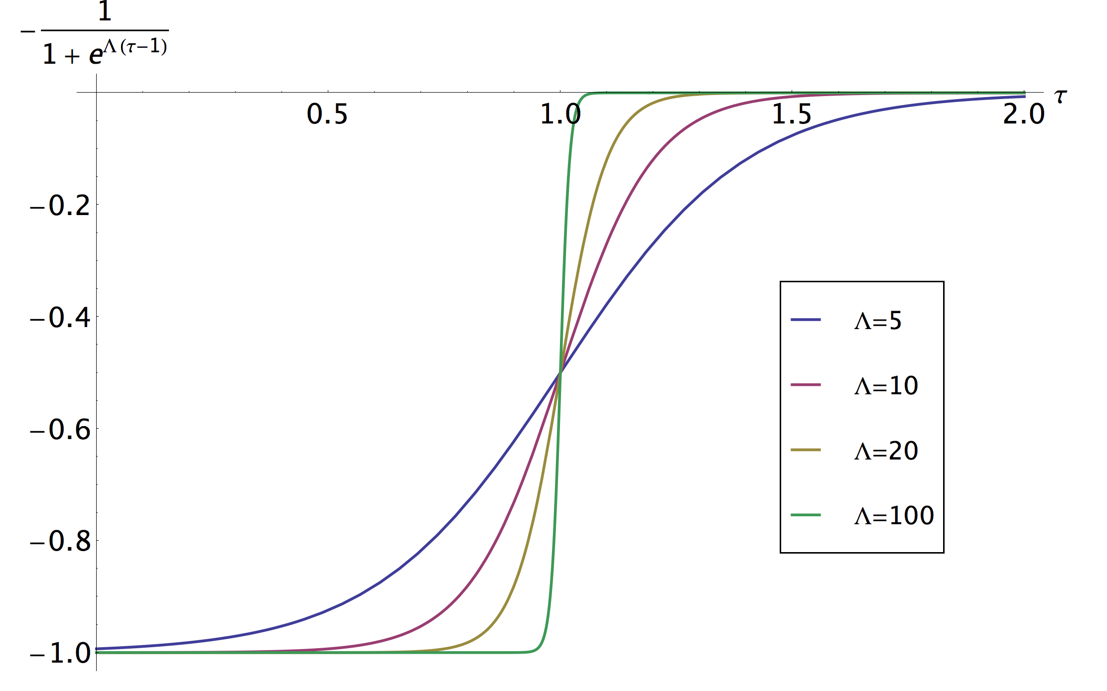
Figure 1: Plot of the approximate potential $\frac{1}{1+e^{\Lambda(\tau-1)}}$. As $\Lambda=-\log x$ is increased, the potential approaches a finite depth square well.

The Schrödinger equation with the potential (11) can be solved exactly with boundary conditions

$$\psi^{\prime}(0)=0,\qquad\psi(+\infty)=0.$$ (12)

The solution vanishing at infinity is (up to a complex normalization constant)

$$\psi(\tau)=y^{\frac{i}{2}\,\beta}\,\frac{(\Omega+i\,\beta)\,\Gamma(\frac{\Omega+i\,\beta}{2})^{2}}{\Gamma(1+i\,\beta)}\,{}_{2}F_{1}\bigg{(}\frac{-\Omega+i\,\beta}{2},\frac{\Omega+i\,\beta}{2},1+i\,\beta;-y\bigg{)}-\text{c.c}.$$ (13)

where

$$y=x\,e^{\Lambda\,\tau},\qquad\beta=\sqrt{\kappa\,x-\Omega^{2}}.$$ (14)

Imposing the second boundary condition $\psi^{\prime}(0)=0$ and neglecting all terms that vanish as $x\to 0$ faster than any power of $\log x$, we arrive at the master equation

$$\boxed{2\,\cos(\tfrac{1}{2}\,\Lambda\,\beta)=\frac{\beta+i\,\Omega}{\beta-i\,\Omega}\,\frac{\Gamma(1+i\,\beta)}{\Gamma(1-i\,\beta)}\,\bigg{[}\frac{\Gamma(\frac{\Omega-i\,\beta}{2})}{\Gamma(\frac{\Omega+i\,\beta}{2})}\bigg{]}^{2}+\frac{\beta-i\,\Omega}{\beta+i\,\Omega}\,\frac{\Gamma(1-i\,\beta)}{\Gamma(1+i\,\beta)}\,\bigg{[}\frac{\Gamma(\frac{\Omega+i\,\beta}{2})}{\Gamma(\frac{\Omega-i\,\beta}{2})}\bigg{]}^{2}.}$$ (15)

Expansion of (15) is quite simple. One simply writes $\Omega$ as a power series in $\kappa$ (actually $\kappa\,x$) starting at order $\mathcal{O}(\kappa)$, and uses the definition of $\beta$ in (14). This procedure fully reproduces the six loop results in (2), and can be extended at higher orders. For instance, at seven loops, we find the new expression

$$\Omega_{7}(x)\,=\,-\frac{2041856}{173745}\,\log^{13}x-\frac{4083712\,\pi^{2}}{93555}\,\log^{11}x-\frac{678016}{4725}\,\zeta_{3}\,\log^{10}x$$

$$\quad-\frac{2482048\,\pi^{4}}{42525}\,\log^{9}x-\bigg{(}\frac{339008}{945}\,\pi^{2}\,\zeta_{3}+\frac{170176}{315}\,\zeta_{5}\bigg{)}\,\log^{8}x-\bigg{(}\frac{34304}{63}\,\zeta_{3}^{2}$$

$$\quad+\frac{10054144\,\pi^{6}}{297675}\bigg{)}\,\log^{7}x-\bigg{(}\frac{2560}{9}\,\pi^{4}\,\zeta_{3}+\frac{4096}{5}\,\pi^{2}\,\zeta_{5}+\frac{4288\,\zeta_{7}}{3}\bigg{)}\,\log^{6}x$$

$$\quad-\bigg{(}\frac{34304}{45}\,\pi^{2}\,\zeta_{3}^{2}+\frac{42752}{15}\,\zeta_{3}\,\zeta_{5}+\frac{341456\,\pi^{8}}{42525}\bigg{)}\,\log^{5}x-\bigg{(}\frac{5888}{9}\,\zeta_{3}^{3}$$

$$\quad+\frac{221888\,\pi^{6}\,\zeta_{3}}{2835}+\frac{14768}{45}\,\pi^{4}\,\zeta_{5}+\frac{3344}{3}\,\pi^{2}\,\zeta_{7}+\frac{22384\,\zeta_{9}}{9}\bigg{)}\,\log^{4}x$$

$$\quad-\bigg{(}\frac{11584}{45}\,\pi^{4}\,\zeta_{3}^{2}+2112\,\zeta_{5}^{2}+\frac{5504}{3}\,\pi^{2}\,\zeta_{3}\,\zeta_{5}+4224\,\zeta_{3}\,\zeta_{7}$$

$$\quad+\frac{95008\,\pi^{10}}{155925}\bigg{)}\,\log^{3}x-\bigg{(}\frac{2944}{9}\,\pi^{2}\,\zeta_{3}^{3}+\frac{80048\,\pi^{8}\,\zeta_{3}}{14175}+2432\,\zeta_{3}^{2}\,\zeta_{5}$$

$$\quad+\frac{4256}{135}\,\pi^{6}\,\zeta_{5}+\frac{808}{5}\,\pi^{4}\,\zeta_{7}+\frac{6656}{9}\,\pi^{2}\,\zeta_{9}+2584\,\zeta_{11}\bigg{)}\,\log^{2}x$$ (16)

$$\quad-\bigg{(}128\,\zeta_{3}^{4}+\frac{5056}{315}\,\pi^{6}\,\zeta_{3}^{2}+384\,\pi^{2}\,\zeta_{5}^{2}+\frac{2528}{15}\,\pi^{4}\,\zeta_{3}\,\zeta_{5}$$

$$\quad+768\,\pi^{2}\,\zeta_{3}\,\zeta_{7}+2592\,\zeta_{5}\,\zeta_{7}+2656\,\zeta_{3}\,\zeta_{9}+\frac{43688\,\pi^{12}}{6081075}\bigg{)}\,\log x-\frac{608}{45}\,\pi^{4}\,\zeta_{3}^{3}$$

$$\quad-672\,\zeta_{3}\,\zeta_{5}^{2}-\frac{5528\,\pi^{10}\,\zeta_{3}}{155925}-192\,\pi^{2}\,\zeta_{3}^{2}\,\zeta_{5}-\frac{248\,\pi^{8}\,\zeta_{5}}{945}-672\,\zeta_{3}^{2}\,\zeta_{7}-\frac{68\,\pi^{6}\,\zeta_{7}}{35}$$

$$\quad-\frac{136\,\pi^{4}\,\zeta_{9}}{9}-124\,\pi^{2}\,\zeta_{11}-1260\,\zeta_{13}+\mathcal{O}(x).$$

The similar 8-loop result is collected in App. (A).

2.1 Generating functions and transcendentality expansion

Given the plain structure in (2) and (2), it is tempting to understand what is the generating function for the various coefficients $b^{(n)}_{k}$, see (4). This may be achieved by means of the following trick. The $\Gamma$ functions in the r.h.s. of (15) are the only source of transcendental contributions. We can consider the r.h.s. of (15) with fixed ratio $\beta/\Omega$ and expand at small $\beta$ the resulting expression. This expansion reads

$$\text{ r.h.s. of (\ref{2.9})}=2\,\frac{\beta^{2}-\Omega^{2}}{\beta^{2}+\Omega^{2}}-\frac{2\,\beta^{2}\,\Omega^{2}}{3\,(\beta^{2}+\Omega^{2})}\,\bm{\pi^{2}}+2\,\beta^{2}\,\Omega\,\,\bm{\zeta_{3}}$$ (17)

$$+\frac{\beta^{2}\,\Omega^{2}\,(\Omega^{2}-\beta^{2})}{60\,(\beta^{2}+\Omega^{2})}\,\bm{\pi^{4}}+\frac{1}{6}\,\beta^{2}\Omega\,\bigg{[}\bm{\pi^{2}\,\zeta_{3}}(\beta^{2}-\Omega^{2})+3\,\bm{\zeta_{5}}\,(\Omega^{2}-3\,\beta^{2})\bigg{]}+$$

$$+\frac{\beta^{2}}{7560\,(\beta^{2}+\Omega^{2})}\,\bigg{[}\bm{\pi^{6}}\,\Omega^{2}\,(5\beta^{4}+16\beta^{2}\Omega^{2}+5\Omega^{4})-1890\,\bm{\zeta_{3}^{2}}\,(\beta^{2}-\Omega^{2})\,(\beta^{2}+\Omega^{2})^{2}\bigg{]}$$

$$-\frac{\beta^{2}\Omega}{360}\,\bigg{[}-45\,\bm{\zeta_{7}}\,(\Omega^{2}-3\beta^{2})^{2}+15\,\bm{\pi^{2}\zeta_{5}}\,(3\beta^{4}-4\beta^{2}\Omega^{2}+\Omega^{4})$$

$$\qquad\qquad+\bm{\pi^{4}\zeta_{3}}\,(\beta^{4}+8\beta^{2}\Omega^{2}+\Omega^{4})\bigg{]}+\cdots,$$

and additional contributions may be obtained with no problems. In (17), we have written in bold face the transcendental constants. The terms in (17) are naturally ordered by increasing transcendentality degree (we remind that $\pi^{2n}$ and $\zeta_{n}$ contribute $n$ units). This means that we can decompose $\Omega$ as a sum of contributions of increasing degree and solve (15) for each of them. The first term in (17) has degree zero and gives the leading order condition

$$\sqrt{\kappa\,x-\omega^{2}_{0}}\,\tan\bigg{(}\frac{\log x}{2}\,\sqrt{\kappa\,x-\omega^{2}_{0}}\bigg{)}+\omega_{0}=0.$$ (18)

Expanding (18) at small $x$ gives

$$\begin{split}\omega_{0}&=-2\,x\,\log x\,\frac{\kappa}{4}+\frac{4}{3}\,x^{2}\,\log^{3}x\,\bigg{(}\frac{\kappa}{4}\bigg{)}^{2}-\frac{8}{5}\,x^{3}\,\log^{5}x\,\bigg{(}\frac{\kappa}{4}\bigg{)}^{3}+\frac{736}{315}\,x^{4}\,\log^{7}x\,\bigg{(}\frac{\kappa}{4}\bigg{)}^{4}\\ &-\frac{2144}{567}\,x^{5}\,\log^{9}x\,\bigg{(}\frac{\kappa}{4}\bigg{)}^{5}+\frac{339008}{51975}\,x^{6}\,\log^{11}x\,\bigg{(}\frac{\kappa}{4}\bigg{)}^{6}+\cdots.\end{split}$$ (19)

Comparing (19) with (2), we see that the compact relation (18) captures all the leading logarithms for $x\to 0$ and, of course, may be extended at arbitrarily higher order with minor effort. A simple way to do this is to notice that (18) implies the following differential constraint for $\omega_{0}=f(\kappa\,x)$ with

$$2\,\text{k}\,\bigg{[}\log x\,f(\text{k})-2\bigg{]}\,f^{\prime}(\text{k})+2\,f(\text{k})-\log x\,\text{k}=0.$$ (20)

Starting with $f(\text{k})=-1/2\,\log x\,\text{k}+\cdots$, one gets from (20) a simple recursion for the coefficients in (19). The convergence properties of the expansion (19) are discussed in App. (B). To illustrate what happens beyond the leading (rational) logarithms, we present the contributions with transcendentality up to 5, i.e. proportional to $\pi^{2},\zeta_{3}$, $\pi^{4}$, $\zeta_{5}$, and $\pi^{2}\,\zeta_{3}$ as an illustrative example. After some some straightforward manipulations, we get from (15) using (17)

$$\Omega =\omega_{0}+\bm{\zeta_{2}}\,\frac{\omega_{0}\,(\kappa\,x-\omega^{2}_{0})}{\omega_{0}\,\log x-2}-\bm{\zeta_{3}}\,\frac{\kappa\,x\,(\kappa\,x-\omega^{2}_{0})}{2\,(\omega_{0}\,\log x-2)}-\bm{\zeta_{4}}\,\frac{\omega_{0}\,(\kappa\,x-\omega_{0}^{2})}{4\,(\omega_{0}\,\log x-2)^{3}}\times$$ (21)

$$\bigg{[}\log^{2}x\,\omega_{0}^{2}\,(\kappa\,x-2\,\omega_{0}^{2})-\log x\,\omega_{0}\,(9\,\kappa\,x-28\,\omega_{0}^{2})+2\,(12\,\kappa\,x-29\,\omega_{0}^{2})\bigg{]}$$

$$+\bm{\zeta_{5}}\,\frac{\kappa\,x\,(3\,\kappa\,x-4\,\omega_{0}^{2})\,(\kappa\,x-\omega_{0}^{2})}{8\,(\omega_{0}\,\log x-2)}+\bm{\pi^{2}\,\zeta_{3}}\,\frac{\kappa\,x\,(\kappa\,x-\omega_{0}^{2})(2\,\kappa\,x+3\,\log x\,\omega_{0}^{3}-8\,\omega_{0}^{2})}{12\,(\omega_{0}\,\log x-2)^{3}}+\cdots\ ,$$

where again we have written in bold face the transcendental constants. Dots in (21) stand for terms with transcendentality $\text{d}>5$. This is a compact generating function for the considered terms. If we plug (19) into (21), we recover the associated contributions in (2). For instance, one obtains immediately the following expansions valid up to 14 loops (recall that $\Omega_{7}$ and $\Omega_{8}$ are given in (2) and (A) respectively)

$$\Omega_{9}\,=\, -\frac{3863148032}{92775375}\,\log^{17}x-\frac{61810368512}{49116375}\,\zeta_{2}\,\log^{15}x-\frac{27910995968}{42567525}\,\zeta_{3}\,\log^{14}$$

$$-\frac{8434823168}{225225}\,\zeta_{4}\,\log^{13}-\left(\frac{3488874496}{1403325}\pi^{2}\zeta_{3}+\frac{1265275904}{467775}\zeta_{5}\right)\log^{12}x+\dots$$

$$\Omega_{10}\,=\, \frac{30013777507328}{371231385525}\,\log^{19}x+\frac{30013777507328}{10854718875}\,\zeta_{2}\,\log^{17}x+\frac{7726296064}{5457375}\,\zeta_{3}\,\log^{16}x$$

$$+\frac{1569005477888}{16372125}\,\zeta_{4}\,\log^{15}x+\left(\frac{61810368512}{9823275}\,\pi^{2}\zeta_{3}+\frac{36584833024}{6081075}\zeta_{5}\right)\log^{14}x+\dots,$$

$$\Omega_{11}\,=\, -\frac{2824240881547264}{17717861581875}\,\log^{21}x-\frac{11296963526189056}{1856156927625}\,\zeta_{2}\,\log^{19}x$$

$$-\frac{60027555014656}{19538493975}\,\zeta_{3}\,\log^{18}x-\frac{871572721432576}{3618239625}\,\zeta_{4}\,\log^{17}x$$

$$-\left(\frac{30013777507328}{1915538625}\pi^{2}\zeta_{3}+\frac{8533890092032}{638512875}\zeta_{5}\right)\log^{16}x+\dots,$$

$$\Omega_{12}\,=\, \frac{747290210255691776}{2348038513445625}\,\log^{23}+\frac{373645105127845888}{27842353914375}\,\zeta_{2}\,\log^{21}x$$ (22)

$$+\frac{5648481763094528}{843707694375}\,\zeta_{3}\,\log^{20}x+\frac{123198569973917696}{206239658625}\,\zeta_{4}\,\log^{19}x$$

$$+\left(\frac{11296963526189056}{293077409625}\pi^{2}\zeta_{3}+\frac{170578599356416}{5746615875}\zeta_{5}\right)\,\log^{18}x\dots,$$

$$\Omega_{13}\,=\, -\frac{182689999846621413376}{284473896821296875}\,\log^{25}x-\frac{1461519998772971307008}{49308808782358125}\,\zeta_{2}\,\log^{23}x$$

$$-\frac{1494580420511383552}{102088631019375}\,\zeta_{3}\,\log^{22}x-\frac{95233730539048824832}{64965492466875}\,\zeta_{4}\,\log^{21}x$$

$$-\left(\frac{373645105127845888}{3977479130625}\pi^{2}\zeta_{3}+\frac{611963637598932992}{9280784638125}\zeta_{5}\right)\,\log^{20}x+\dots,$$

$$\Omega_{14}\,=\, \frac{242473345197975650369536}{185436341599368234375}\,\log^{27}x+\frac{242473345197975650369536}{3698160658676859375}\,\zeta_{2}\,\log^{25}x$$

$$+\frac{365379999693242826752}{11378955872851875}\,\zeta_{3}\,\log^{24}x+\frac{58635553926660888199168}{16436269594119375}\,\zeta_{4}\,\log^{23}$$

$$+\left(\frac{1461519998772971307008}{6431583754220625}\pi^{2}\zeta_{3}+\frac{62835830527435194368}{428772250281375}\zeta_{5}\right)\log^{22}x+\dots.$$

and so on. Having long series of this kind allows to recognize some interesting pattern. For instance, the ratio of the NLO logarithm coefficient (proportional to $\zeta_{2}$) to the coefficient of the LO logarithm is simply, see (4)

$$\frac{b^{(n)}_{3}}{b^{(n)}_{1}}=\frac{2\,(n-1)(2n-1)}{n}\,\zeta_{2},$$ (23)

where $n$ is the loop order. This relation can be proved rigorously starting from (20) and converting the factors in (23) into differential operators $n\to\kappa\partial_{\kappa}$. Another simple relation concerns the ratio of the NNLO logarithm coefficient (proportional to $\zeta_{3}$),

$$\frac{b_{4}^{(n)}}{b_{1}^{(n-1)}}=2\,(3-2\,n)\,\zeta_{3},$$ (24)

where the shift in the index of $b_{1}$ is a non trivial fact. The vanishing $b_{2}^{(n)}=0$ and the uniform transcendentality property of the expansion (4) are thus direct consequences of the relation (17) since all coefficients in (19) are rational, given (20). As a final remark, we notice that the leading order equation (18) is familiar from the discussion of elementary quantum mechanics in a one-dimensional finite well. This is not accidental and the relation is fully spelled out in App. (C).

3 Higher-order expansion at small $\phi$

To study the problem (3) at small $\phi$, we begin by setting

$$y=\frac{1}{\cosh w+1}$$ (25)

The expansion of the potential is polynomial in $y$

$$\frac{1}{\cosh w+\cos\phi}=y+\frac{y^{2}}{2}\,\phi^{2}+\bigg{(}\frac{y^{3}}{4}-\frac{y^{2}}{24}\bigg{)}\,\phi^{4}+\bigg{(}\frac{y^{4}}{8}-\frac{y^{3}}{24}+\frac{y^{2}}{720}\bigg{)}\,\phi^{6}+\cdots.$$ (26)

The kinetic term is also simple

$$\psi^{\prime\prime}(w)=y^{2}\,(1-2\,y)\,\psi^{\prime\prime}(y)+y\,(1-3\,y)\,\psi^{\prime}(y).$$ (27)

The exact ground state wavefunction at $\phi=0$ is known and reads

$$\psi_{0}(y)=y^{\Omega/2},\qquad\text{with}\qquad\kappa=4\,\Omega\,(\Omega+1).$$ (28)

We now make the educated perturbative Ansatz

$$\begin{split}\psi_{0}(y,\phi)&=y^{\Omega/2}\,\bigg{(}1+\sum_{n=1}^{\infty}f_{n}(y)\,\phi^{2n}\bigg{)},\qquad\kappa=4\,\Omega\,(\Omega+1)+\sum_{n=1}^{\infty}\delta\kappa_{n}(\Omega)\,\phi^{2n},\end{split}$$ (29)

where $\delta\kappa_{n}(\Omega)$ are functions of the ground state energy $\Omega$.

We emphasize that it is crucial to set up the perturbative expansion according to (29), i.e. expanding $\kappa$, instead of writing a more natural perturbative expansion of $\Omega$ as a function of $\kappa$. This has the advantage that the unperturbed ground state in (28) – appearing as a factor in (29) – is not changed during the procedure. Replacing (29) into the Schrödinger equation, we get

$$y^{-\Omega}\,\sqrt{1-2\,y}\,\frac{d}{dy}\bigg{[}y^{\Omega+1}\,\sqrt{1-2y}\,f_{1}^{\prime}(y)\bigg{]}+\frac{y}{4}\,\Omega\,(\Omega+1)+\frac{1}{8}\,\delta\kappa_{1}=0,$$ (30)

$$y^{-\Omega}\,\sqrt{1-2\,y}\,\frac{d}{dy}\bigg{[}y^{\Omega+1}\,\sqrt{1-2y}\,f_{2}^{\prime}(y)\bigg{]}+\frac{y}{4}\,\Omega\,(\Omega+1)+f_{1}(y)\,\bigg{(}\frac{\delta\kappa_{1}}{8}+\frac{y}{4}\,\Omega\,(\Omega+1)\bigg{)}$$

$$\qquad+\frac{1}{48}\,y\,(6y-1)\,\Omega\,(\Omega+1)+\frac{1}{8}\delta\kappa_{2}+\frac{y}{16}\,\delta\kappa_{1}=0,$$

$$\qquad\qquad\cdots$$

and so on. Clearly, the equations in the chain (30) can be integrated one after the other. Imposing boundary conditions, we fix the coefficients $\delta\kappa_{n}$. Actually, inspection of the results shows that the general form of the corrected wave-function is

$$\boxed{\begin{split}\psi_{0}(y,\phi)&=y^{\Omega/2}\,\bigg{(}1+\sum_{n=1}^{\infty}\phi^{2n}\,\sum_{k=1}^{n}a_{n,k}\,y^{k}\bigg{)}.\end{split}}$$ (31)

In other words, the corrections $f_{n}(y)$ are simple polynomials in $y$ ! This remarkable feature is recurrent in quantum mechanical problems with a perturbation in the form of a polynomial, see the original proposal in dalgarno1956perturbation or, for instance, fernandez2000introduction . The explicit solution for the first three non trivial corrections is

$$f_{1}(y)= y\frac{\,\Omega(\,\Omega+1)}{8\,\Omega+12},$$

$$f_{2}(y)= y^{2}\frac{\,\Omega(\,\Omega+1)(\,\Omega+2)(\,\Omega+3)}{32(2\,\Omega+3)(2\,\Omega+5)}-y\frac{\,\Omega(\,\Omega+1)\left(8\,\Omega^{3}+41\,\Omega^{2}+63\,\Omega+27\right)}{48(2\,\Omega+3)^{3}(2\,\Omega+5)},$$ (32)

$$f_{3}(y)= y^{3}\frac{\,\Omega(\,\Omega+1)(\,\Omega+2)(\,\Omega+3)(\,\Omega+4)(\,\Omega+5)}{384(2\,\Omega+3)(2\,\Omega+5)(2\,\Omega+7)}-$$

$$\qquad y^{2}\frac{\,\Omega(\,\Omega+1)(\,\Omega+2)(\,\Omega+3)\left(8\,\Omega^{3}+49\,\Omega^{2}+87\,\Omega+45\right)}{192(2\,\Omega+3)^{3}(2\,\Omega+5)(2\,\Omega+7)}+$$

$$\qquad y\frac{\,\Omega(\,\Omega+1)\left(64\,\Omega^{6}+738\,\Omega^{5}+3383\,\Omega^{4}+7803\,\Omega^{3}+9378\,\Omega^{2}+5454\,\Omega+1215\right)}{1440(2\,\Omega+3)^{5}(2\,\Omega+5)(2\,\Omega+7)}.$$ (33)

and

$$\delta\kappa_{1}= -\frac{2\,\Omega(\,\Omega+1)^{2}}{2\,\Omega+3},$$

$$\delta\kappa_{2}= \frac{\,\Omega(\,\Omega+1)^{2}\left(8\,\Omega^{3}+41\,\Omega^{2}+63\,\Omega+27\right)}{6(2\,\Omega+3)^{3}(2\,\Omega+5)},$$ (34)

$$\delta\kappa_{3}= -\frac{\,\Omega(\,\Omega+1)^{2}\left(64\,\Omega^{6}+738\,\Omega^{5}+3383\,\Omega^{4}+7803\,\Omega^{3}+9378\,\Omega^{2}+5454\,\Omega+1215\right)}{180(2\,\Omega+3)^{5}(2\,\Omega+5)(2\,\Omega+7)}.$$

The expansion of $\kappa$ in (29), may be turned into an expansion of $\Omega$ according to

$$\,\Omega= \frac{t-1}{2}+\frac{(t-1)(t+1)^{2}\phi^{2}}{16t(t+2)}+$$

$$\frac{(t-1)(t+1)^{2}\left(5\,t^{5}+40\,t^{4}+97\,t^{3}+68\,t^{2}+18\,t+24\right)\phi^{4}}{768t^{3}(t+2)^{3}(t+4)}+$$ (35)

$$\frac{(t-1)(t+1)^{2}}{92160t^{5}(t+2)^{5}(t+4)^{2}(t+6)}\left(61\,t^{11}+1342\,t^{10}+12170\,t^{9}+58906\,t^{8}+163733\,t^{7}+\right.$$

$$\qquad\left.259846\,t^{6}+222676\,t^{5}+107946\,t^{4}+65040\,t^{3}+57960\,t^{2}+37440\,t+17280\right)\phi^{6}+\dots$$

where $t=\sqrt{\kappa+1}$. The general structure of the higher order corrections is

$$\Omega=\sum_{n=1}^{\infty}\mathcal{P}_{n}(t)\mathcal{D}_{n}(t)\phi^{2n},$$ (36)

where $\mathcal{D}_{n}(t)$ is the rational function

$$\begin{split}\mathcal{D}_{n}(t)=\frac{(t+2)^{2}(t-1)(t+1)^{2}}{\left[2^{2(n+1)-1}t^{n-2}\Gamma(2(n+1)-1)\right]\prod_{j=1}^{n+1}t(t+2)(2j+t)^{-j+n+1}},\end{split}$$ (37)

and $\mathcal{P}_{n}(t)$ are polynomials. The first cases are collected in App. (D). They have an increasing complexity, but may be generated quite easily by the above procedure.

3.1 A cross-check at large $\kappa$

The expansion (3) may be checked at weak coupling, i.e. in the limit $\kappa\to 0$, using the six-loop expressions derived in Henn:2012qz . At strong coupling, we can evaluate systematically the perturbative expansion of the (ladder) cusp anomaly for any $\phi$. This can be achieved by the same strategy described in the previous section, i.e. by an Ansatz similar to (29). We begin by multiplying the Schrödinger equation by $\mu^{2}/\kappa$ with $\mu^{2}=4\,\sqrt{\kappa}(\cos\phi+1)$. After a rescaling $x=\mu\,X/\sqrt{\kappa}$, we obtain

$$\begin{split}&\bigg{(}-\frac{d^{2}}{dX^{2}}+\mathcal{V}(X,\phi)\bigg{)}\,\psi(X)=E\,\psi(X),\\ &\mathcal{V}(X,\phi)=-\frac{\sqrt{\kappa}}{2}+X^{2}+\frac{\cos\phi-5}{3\,\sqrt{\kappa}}\,X^{4}+\frac{123-56\,\cos\phi+\cos(2\phi)}{45\,\kappa}\,X^{6}+\dots,\\ E&=-\frac{\cos\phi+1}{\sqrt{\kappa}}\,\Omega^{2}.\end{split}$$ (38)

The perturbative correction to the ground state energy $E$ of the (formal) problem

$$-\psi^{\prime\prime}(X)+\bigg{(}X^{2}+\sum_{n=2}^{\infty}\varepsilon^{n-1}\,c_{2n}\,X^{2n}\bigg{)}\,\psi(X)=E\,\psi(X),$$ (39)

can be found efficiently by the Ansatz

$$\psi(X)=e^{-\frac{X^{2}}{2}}\bigg{(}1+\sum_{n=1}^{\infty}p_{n}(X)\,\varepsilon^{n}\bigg{)},$$ (40)

where $p_{n}(X)$ is an even polynomial with degree $4n$ and without constant term. The first three cases are explicitly

$$p_{1}(X) =-\frac{3c_{4}X^{2}}{8}-\frac{c_{4}X^{4}}{8},$$ (41)

$$p_{2}(X) =\frac{3}{32}\left(7c_{4}^{2}-10c_{6}\right)X^{2}+\frac{1}{128}\left(31c_{4}^{2}-40c_{6}\right)X^{4}+\frac{1}{192}\left(13c_{4}^{2}-16c_{6}\right)X^{6}+\frac{1}{128}c_{4}^{2}X^{8},$$

$$p_{3}(X) =-\frac{3}{128}\left(111c_{4}^{3}-240c_{6}c_{4}+140c_{8}\right)X^{2}+\frac{1}{256}\left(-243c_{4}^{3}+510c_{6}c_{4}-280c_{8}\right)X^{4}$$

$$+\frac{1}{3072}\,\left(-813c_{4}^{3}+1680c_{6}c_{4}-896c_{8}\right)\,X^{6}+\frac{1}{1024}\,\left(-47c_{4}^{3}+104c_{6}c_{4}-64c_{8}\right)\,X^{8}$$

$$-\frac{c_{4}}{3072}\,\left(17c_{4}^{2}-32c_{6}\right)\,X^{10}-\frac{c_{4}^{3}}{3072}\,X^{12},$$

and lead to the perturbed energy

$$E=1+\frac{3\,c_{4}}{4}\,\varepsilon-\frac{3}{16}\,(7\,c_{4}^{2}-10\,c_{6})\,\varepsilon^{2}+\frac{3}{64}\,(111\,c_{4}^{3}-240\,c_{4}\,c_{6}+140\,c_{8})\,\varepsilon^{3}+\cdots.$$ (42)

The associated expansion of the cusp anomalous dimension is therefore

$$\begin{split}\Gamma^{\text{lad}}&=\frac{\sqrt{\kappa}}{2\,\cos\frac{\phi}{2}}\bigg{[}1-\frac{1}{\sqrt{\kappa}}+\frac{3-\cos\phi}{4\,\kappa}+\frac{1}{\kappa^{3/2}}\,\frac{-21+20\,\cos\phi+\cos(2\phi)}{32}\\ &+\frac{1}{\kappa^{2}}\,\frac{290-317\,\cos\phi-2\,\cos(2\phi)-3\,\cos(3\phi)}{256}+\cdots\bigg{]},\end{split}$$ (43)

in full agreement with what one finds by expanding (3) at large $t$.

3.2 Numerical analysis

In this section, we compare the exact numerical solution of the Schrödinger problem (3) with the small $\phi$ expansion of its ground state energy, see (36). We shall consider three reference values $\kappa=1,2,5$ and explore convergence with respect to $\phi$ in the physical interval $0\leq\phi<\pi$. The first comparison is with the naive partial sums of (36), ( recall that $\Gamma^{\rm lad}=-\Omega$ )

$$\Omega_{N}=\sum_{n=1}^{N}\,\mathcal{P}_{n}\,\mathcal{D}_{n}\,\phi^{2n}.$$ (44)

This is shown in the left panel of Fig. (2).

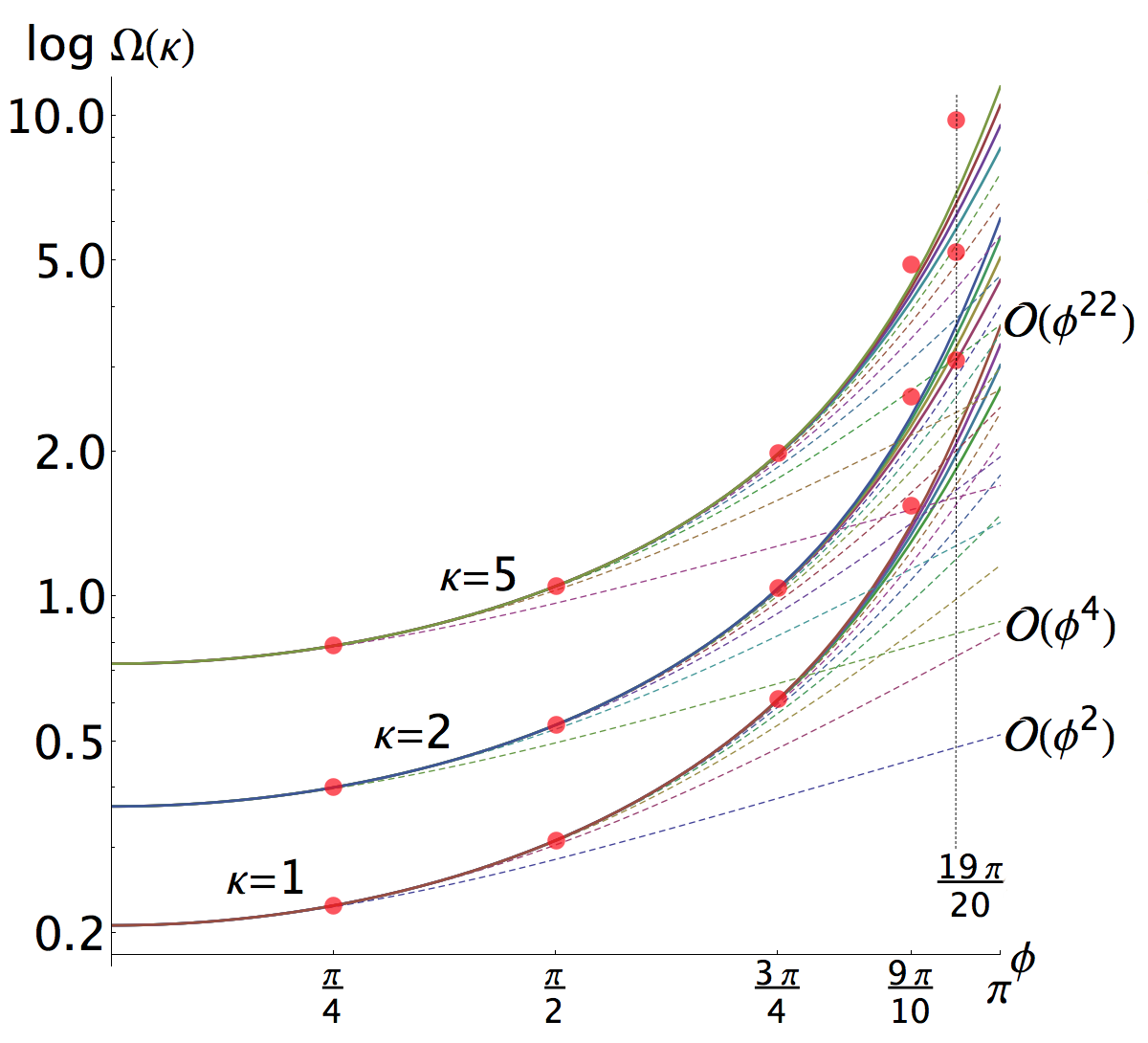
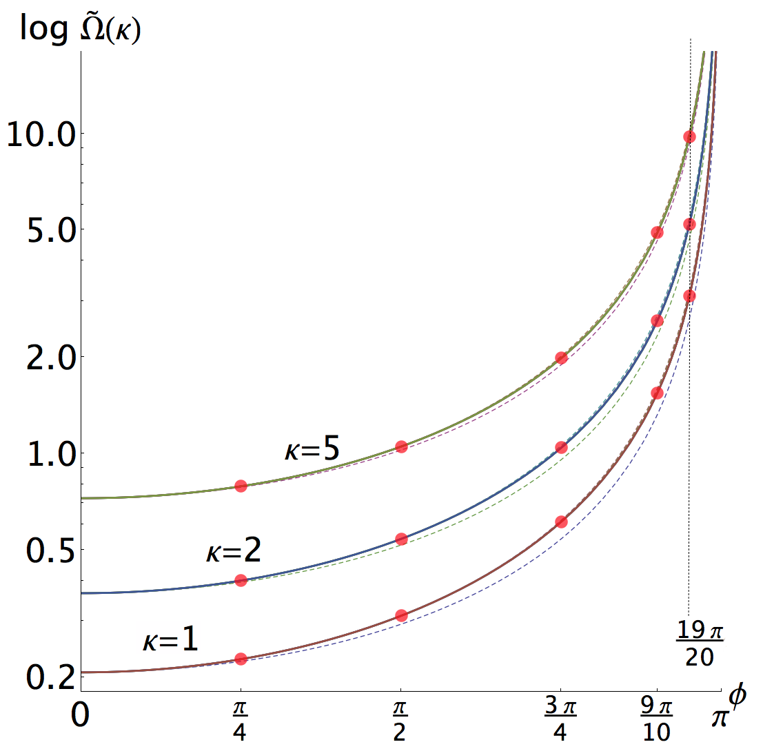
Figure 2: The plots show the convergence of the perturbative expansion of $\Omega$ at small $\phi$ for $\kappa=1,2,5$. The many thin dashed lines show results with lower values of $N$ in (44) (left panel) and (45) (right panel). The four red dots are the (numerical) exact values of $\Omega$ obtained solving numerically the Schrödinger equation at $\phi=\tfrac{\pi}{4},\tfrac{\pi}{2},\tfrac{3\,\pi}{4}$, $\tfrac{9\,\pi}{10}$, and $\tfrac{19\,\pi}{20}$, see also Tab. (1).

One sees that including terms up to $N=20$, there is convergence to the exact numerical value at least for $\phi$ not too close to $\pi$. As $\phi\to\pi$, convergence slows down and the series expansion cannot provide an accurate estimate of the correct (ladder) cusp anomaly. This is clearly illustrated by the points at $\phi=\tfrac{19\pi}{20}$. However, the strong coupling expansion (43) suggests that the singularity at $\phi=\pi$ is simply due to an overall factor $1/\cos(\phi/2)$. From the physical point of view, the $\phi\to\pi$ limit is a flat space limit where that singularity is nothing but the overall scale $1/r$ in the quark-antiquark at distance $r\sim 2\,\cos(\frac{\phi}{2})$ Correa:2012nk . Hence, we also compare the numerical values of the cusp anomaly with the improved summation

$$\widetilde{\Omega}_{N}=\frac{1}{\cos\frac{\phi}{2}}\left[\cos\frac{\phi}{2}\sum_{n=1}^{N}\,\mathcal{P}_{n}\,\mathcal{D}_{n}\,\phi^{2n}\right]_{\text{truncated at $\phi^{2N}$}}.$$ (45)

The right panel of Fig. (2) shows that this is a major improvement. The convergence in $N$ is now greatly increased and accurate results are obtained even quite near the singular point $\phi=\pi$. This is illustrated in a more quantitative way in Tab. (1) where we collect some reference numerical values shown in Fig. (2). In all cases, the relative accuracy of (45) is well below the $10^{-3}$ level.

$$\begin{array}[]{|cc|c|c|c|}\hline\cr\kappa&\phi&\Omega\,\,\text{exact}&\Omega_{N=20}&\widetilde{\Omega}_{N=20}\\ \hline\cr 1&\frac{\pi}{4}&0.2277386205&\;{\color[rgb]{0,0,1}0.2277386205}&\;{\color[rgb]{0,0,1}0.2277386205}\\ 1&\frac{\pi}{2}&0.3112053734&\;{\color[rgb]{0,0,1}0.3112053}487&\;{\color[rgb]{0,0,1}0.311205373}3\\ 1&\frac{3\pi}{4}&0.6121866441&\;{\color[rgb]{0,0,1}0.61}14749855&\;{\color[rgb]{0,0,1}0.61218}58951\\ 1&\frac{9\pi}{10}&1.546211922&\;{\color[rgb]{0,0,1}1}.4159044310&\;{\color[rgb]{0,0,1}1.546}0568021\\ 1&\frac{19\pi}{20}&3.101434441&\;2.17175679664&\;{\color[rgb]{0,0,1}3.10}02145584\\ \hline\cr 2&\frac{\pi}{4}&0.4008519359&\;{\color[rgb]{0,0,1}0.400851935}8&\;{\color[rgb]{0,0,1}0.4008519359}\\ 2&\frac{\pi}{2}&0.5409421028&\;{\color[rgb]{0,0,1}0.540942}0614&\;{\color[rgb]{0,0,1}0.540942102}7\\ 2&\frac{3\pi}{4}&1.042364136&\;{\color[rgb]{0,0,1}1.04}11714765&\;{\color[rgb]{0,0,1}1.04236}35475\\ 2&\frac{9\pi}{10}&2.599160526&\;{\color[rgb]{0,0,1}2}.3808426079&\;{\color[rgb]{0,0,1}2.599}0745817\\ 2&\frac{19\pi}{20}&5.199351482&\;3.6420358922&\;{\color[rgb]{0,0,1}5.19}88023024\\ \hline\cr 5&\frac{\pi}{4}&0.7898806509&\;{\color[rgb]{0,0,1}0.789880650}8&\;{\color[rgb]{0,0,1}0.789880650}8\\ 5&\frac{\pi}{2}&1.051108721&\;{\color[rgb]{0,0,1}1.051108}6429&\;{\color[rgb]{0,0,1}1.05110872}06\\ 5&\frac{3\pi}{4}&1.985138624&\;{\color[rgb]{0,0,1}1.98}28960288&\;{\color[rgb]{0,0,1}1.985138}9346\\ 5&\frac{9\pi}{10}&4.899715022&\;{\color[rgb]{0,0,1}4}.489210222&\;{\color[rgb]{0,0,1}4.8997}700298\\ 5&\frac{19\pi}{20}&9.783226208&\;6.8549556957&\;{\color[rgb]{0,0,1}9.783}6202372\\ \hline\cr\end{array}$$

Table 1: This table compares the exact values of $\Omega$ with the approximations in (44) and (45) for $N=20$. The comparison is done at $\kappa=1,2,5$ and various $\phi$. The first column contains the (numerical) exact value corresponding to the red dots in Fig. (2). Digits highlighted in blue are in agreement with the exact solution.

4 Conclusions

In this paper we have considered various properties of the perturbative expansion of the cusp anomalous dimension in $\mathcal{N}=4$ SYM in the (leading order) ladder approximation. We have presented simple algorithms for the higher-order evaluation of the (i) small $x=e^{i\,\phi}$ and (ii) small $\phi$ corrections. In the former case, we showed that all the logarithmic corrections are captured by a Wood-Saxon type solvable problem. Besides, we have shown how to generate all such corrections at higher-orders by compact generating functions that encode them and are naturally organised in increasing transcendentality degree. Our approach explains the remarkable regularities observed in the past. In the small $\phi$ regime, we showed that is possible to work out the quantum mechanical perturbation expansion bypassing the Rayleigh-Schrödinger scheme. This is due to the simple structure of the perturbed wave-function associated with the ground state. Our remark leads to a quite efficient algorithm. The associated long expansion in powers of $\phi$ has been shown to provide, after some educated manipulations, an accurate representation of the ladder cusp anomaly in the whole range of couplings and angles. We believe that it would be very interesting to look at our results from the perspective of the Quantum Spectral Curve by extending the analysis of Gromov:2016rrp to the case of a generic cusp angle $\phi$. Our new results could certainly be useful as a non-trivial check of that method.

Appendix A Complete expression of the eight-loops term $\Omega_{8}$

$$\Omega_{8}(x)\,=\,\frac{13955497984}{638512875}\,\log^{15}x+\frac{1744437248}{18243225}\,\pi^{2}\,\log^{13}x+\frac{4083712}{13365}\,\zeta_{3}\,\log^{12}x$$

$$\quad+\frac{371067328}{2338875}\,\pi^{4}\,\log^{11}x+\left(\frac{8167424\,\pi^{2}\,\zeta_{3}}{8505}+\frac{17188736\,\zeta_{5}}{14175}\right)\log^{10}x$$

$$\quad+\left(\frac{1356032\,\zeta_{3}^{2}}{945}+\frac{110648288\,\pi^{6}}{893025}\right)\log^{9}x+\left(\frac{4964096\,\pi^{4}\,\zeta_{3}}{4725}+\frac{12736\,\pi^{2}\,\zeta_{5}}{5}\right.$$

$$\quad\left.+\frac{378176\,\zeta_{7}}{105}\right)\log^{8}x+\left(\frac{2712064}{945}\,\pi^{2}\,\zeta_{3}^{2}+\frac{2722816\,\zeta_{5}\,\zeta_{3}}{315}+\frac{205490336\,\pi^{8}}{4465125}\right)\,\log^{7}x$$

$$\quad+\left(\frac{68608\,\zeta_{3}^{3}}{27}+\frac{20108288\,\pi^{6}\,\zeta_{3}}{42525}+\frac{124928\,\pi^{4}\,\zeta_{5}}{75}+\frac{205568\,\pi^{2}\,\zeta_{7}}{45}+\frac{1036864\,\zeta_{9}}{135}\right)\,\log^{6}x$$

$$\quad+\left(\frac{5120}{3}\,\pi^{4}\,\zeta_{3}^{2}+\frac{49152}{5}\,\pi^{2}\,\zeta_{5}\,\zeta_{3}+17152\,\zeta_{7}\,\zeta_{3}+8576\,\zeta_{5}^{2}+\frac{17034488\,\pi^{10}}{2338875}\right)\,\log^{5}x$$

$$\quad+\left(\frac{68608}{27}\,\pi^{2}\,\zeta_{3}^{3}+\frac{42752}{3}\,\zeta_{5}\,\zeta_{3}^{2}+\frac{682912\,\pi^{8}\,\zeta_{3}}{8505}+\frac{1050944\,\pi^{6}\,\zeta_{5}}{2835}+\frac{67664\,\pi^{4}\,\zeta_{7}}{45}\right.$$

$$\quad\left.+\frac{135920\,\pi^{2}\,\zeta_{9}}{27}+\frac{33424\,\zeta_{11}}{3}\right)\,\log^{4}x+\left(\frac{11776\,\zeta_{3}^{4}}{9}+\frac{887552\,\pi^{6}\,\zeta_{3}^{2}}{2835}+\frac{118144}{45}\,\pi^{4}\,\zeta_{5}\,\zeta_{3}\right.$$

$$\quad\left.+\frac{26752}{3}\,\pi^{2}\,\zeta_{7}\,\zeta_{3}+\frac{179072\,\zeta_{9}\,\zeta_{3}}{9}+\frac{13376}{3}\,\pi^{2}\,\zeta_{5}^{2}+19584\,\zeta_{5}\,\zeta_{7}+\frac{18213284\,\pi^{12}}{49116375}\right)\,\log^{3}x$$

$$\quad+\left(\frac{23168}{45}\,\pi^{4}\,\zeta_{3}^{3}+5504\,\pi^{2}\,\zeta_{5}\,\zeta_{3}^{2}+12672\,\zeta_{7}\,\zeta_{3}^{2}+12672\,\zeta_{5}^{2}\,\zeta_{3}+\frac{190016\,\pi^{10}\,\zeta_{3}}{51975}+\frac{6704\,\pi^{8}\,\zeta_{5}}{315}\right.$$

$$\quad\left.+\frac{36832\,\pi^{6}\,\zeta_{7}}{315}+\frac{27352\,\pi^{4}\,\zeta_{9}}{45}+2832\,\pi^{2}\,\zeta_{11}+10056\,\zeta_{13}\right)\,\log^{2}x$$

$$\quad+\left(\frac{2944}{9}\,\pi^{2}\,\zeta_{3}^{4}+\frac{9728}{3}\,\zeta_{5}\,\zeta_{3}^{3}+\frac{160096\,\pi^{8}\,\zeta_{3}^{2}}{14175}+\frac{17024}{135}\,\pi^{6}\,\zeta_{5}\,\zeta_{3}+\frac{3232}{5}\,\pi^{4}\,\zeta_{7}\,\zeta_{3}\right.$$

$$\quad\left.+\frac{26624}{9}\,\pi^{2}\,\zeta_{9}\,\zeta_{3}+10336\,\zeta_{11}\,\zeta_{3}+\frac{1616}{5}\,\pi^{4}\,\zeta_{5}^{2}+4752\,\zeta_{7}^{2}+2880\,\pi^{2}\,\zeta_{5}\,\zeta_{7}\right.$$

$$\quad\left.+\frac{29344\,\zeta_{5}\,\zeta_{9}}{3}+\frac{1859138\,\pi^{14}}{638512875}\right)\log x+\frac{256\,\zeta_{3}^{5}}{5}+\frac{10112}{945}\,\pi^{6}\,\zeta_{3}^{3}+864\,\zeta_{5}^{3}+768\,\pi^{2}\,\zeta_{3}\,\zeta_{5}^{2}$$

$$\quad+\frac{87376\,\pi^{12}\,\zeta_{3}}{6081075}+\frac{2528}{15}\,\pi^{4}\,\zeta_{3}^{2}\,\zeta_{5}+\frac{5528\,\pi^{10}\,\zeta_{5}}{51975}+768\,\pi^{2}\,\zeta_{3}^{2}\,\zeta_{7}+5184\,\zeta_{3}\,\zeta_{5}\,\zeta_{7}+\frac{248\,\pi^{8}\,\zeta_{7}}{315}$$

$$\quad+2656\,\zeta_{3}^{2}\,\zeta_{9}+\frac{1156\,\pi^{6}\,\zeta_{9}}{189}+\frac{248\,\pi^{4}\,\zeta_{11}}{5}+420\,\pi^{2}\,\zeta_{13}+\frac{21844\,\zeta_{15}}{5}+\mathcal{O}(x).$$ (46)

Appendix B Convergence of the expansion (19)

The expansion (19) solves (18). The dependence on powers of $x$ and $\log x$ is clearly trivial. Indeed, introducing the variables

$$\kappa=\frac{\overline{\kappa}}{x\,\log^{2}x},\qquad\omega_{0}=\frac{\overline{\omega}_{0}}{\log x},$$ (47)

we can rewrite (18) as

$$\sqrt{\overline{\kappa}-\overline{\omega}_{0}^{2}}\,\tan\bigg{(}\frac{1}{2}\sqrt{\overline{\kappa}-\overline{\omega}_{0}^{2}}\bigg{)}+\overline{\omega}_{0}=0.$$ (48)

This equation admits a solution $\overline{\omega}_{0}(\overline{\kappa})$ that is analytic in a disc of radius $R$. This convergence radius is determined by a branch point at $\overline{\kappa}<0$ where a pair of real roots of (48) coalesce into a pair of complex conjugate roots. Setting $\overline{\kappa}=-R>0$, we determine $R$ by eliminating $w$ in the two equations

$$F(R,w)=w-\sqrt{R+w^{2}}\,\tanh\bigg{(}\frac{1}{2}\sqrt{R+w^{2}}\bigg{)}=0,\qquad\frac{\partial}{\partial w}\,F(R,w)=0.$$ (49)

This gives $w=2$. Then, $R$ is found as the unique positive root of

$$\sqrt{R+4}\,\tanh\bigg{(}\frac{1}{2}\,\sqrt{R+4}\bigg{)}=2,$$ (50)

that is $R=1.756915\dots$ and (19) converges for $|\kappa|<R/(x\,\log^{2}x)$.

Appendix C Small $x$ limit as perturbation around a finite depth well

The potential in (11) can also be split in the following way, where we have again rescaled $w$ by $\log x$ introducing $w=\tau\,\log x$ for $\tau>0$,

$$-\frac{1/x}{\cosh(\tau\,\log x)+\frac{1}{2}(x+x^{-1})}=-2\,\Theta(1-\tau)+\frac{2\,\text{sign}(1-\tau)}{1+e^{-\log x\,|\tau-1|}}+\dots\,.$$ (51)

where $\Theta(\tau)$ is the Heaviside step function. In other words, the potential looks like a Fermi-Dirac distribution. The unperturbed shape is a finite depth well, while the correction – the second term in (51) – captures its deviation in the small strip $\tau-1\sim 1/\log x$.

The solution of the Schrödinger equation for the finite depth well is elementary and reads, for $\tau>0$,

$$\psi(\tau)=\begin{cases}A\,\cos\bigg{(}\log x\,\frac{\sqrt{\kappa\,x-\Omega^{2}}}{2}\,\tau\bigg{)},&0<\tau<1,\\ B\,\exp\bigg{(}\frac{\Omega\,\log x}{2}\,\tau\bigg{)},&\tau>1.\end{cases}$$ (52)

At $\tau=1$, continuity fixes the ratio $A/B$, while continuity of $\psi^{\prime}$ determines the relation between $\Omega$ and $\kappa$ to be precisely (18).

This first approximation may be improved by taking into account the correction in (51). Treating it at first order in perturbation theory amounts to compute its integral times $|\psi(\tau)|^{2}$. But this is accomplished as follows (we omit a trivial factor 2)

$$\begin{split}&\int_{0}^{\infty}d\tau\,\frac{\text{sign}(1-\tau)}{1+e^{-\log x\,|\tau-1|}}\,F(\tau)=\int_{0}^{1}d\tau\,\frac{F(\tau)}{1+e^{-\log x\,(1-\tau)}}-\int_{1}^{\infty}d\tau\,\frac{F(\tau)}{1+e^{-\log x\,(\tau-1)}}\\ &=-\frac{1}{\log x}\,\int_{0}^{-\log x}d\mu\,\frac{F(1+\frac{\mu}{\log x})}{1+e^{\mu}}+\frac{1}{\log x}\,\int_{0}^{\infty}d\mu\,\frac{F(1-\frac{\mu}{\log x})}{1+e^{\mu}}\end{split}$$ (53)

Up to corrections $\mathcal{O}(x)$ – from the upper integration limit in the first integral – we can expand at small $x$ and obtain

$$\begin{split}&\int_{0}^{\infty}d\tau\,\frac{\text{sign}(1-\tau)}{1+e^{-\log x\,|\tau-1|}}\,F(\tau)=\int_{0}^{\infty}d\mu\,\frac{1}{1+e^{\mu}}\\ &\bigg{[}\frac{F(1^{-})-F(1^{+})}{\log x}-\mu\,\frac{F^{\prime}(1^{-})+F^{\prime}(1^{+})}{\log^{2}x}+\mu^{2}\,\frac{F^{\prime\prime}(1^{-})-F^{\prime\prime}(1^{+})}{2\,\log^{3}x}+\cdots\bigg{]}.\end{split}$$ (54)

In our application $F(\tau)=|\psi(\tau)|^{2}$, and $F^{\prime}(\tau)$ are continuous at $\tau=1$, so

$$\begin{split}&\int_{0}^{\infty}d\tau\,\frac{\text{sign}(1-\tau)}{1+e^{-\log x\,|\tau-1|}}\,F(\tau)=-\frac{\zeta_{2}}{\log^{2}x}\,F^{\prime}(1)+\frac{3}{4}\frac{\zeta_{3}}{\log^{3}x}\,[F^{\prime\prime}(1^{-})-F^{\prime\prime}(1^{+})]+\cdots\ .\end{split}$$ (55)

Collecting all pieces, we obtain the simple formula

$$\Omega^{2}_{\text{NNLO}}=\Omega^{2}+4\,\kappa\,x\,(\delta E_{1}+\delta E_{2}^{+}+\delta E_{2}^{-}),$$ (56)

where $\Omega$ is the leading order, i.e. the solution of (18), and

$$\begin{split}\delta E_{1}&=\frac{\zeta_{2}}{2\,\mathcal{N}}\,\frac{\psi(1)\,\psi^{\prime}(1)}{\log^{2}x},\qquad\delta E_{2}^{\pm}=\mp\,\frac{\zeta_{3}}{2\,\mathcal{N}}\frac{\psi(1)\,\psi^{\prime\prime}(1^{\pm})+\psi^{\prime}(1)^{2}}{\log^{3}x},\\ \mathcal{N}&=\int_{0}^{\infty}d\tau\,|\psi(\tau)|^{2}.\end{split}$$ (57)

After some simplification, it is possible to show that (56) is indeed equivalent to the first three terms of (21). In this approach, the appearance of the simple transcendental zeta values if simply due to the elementary integral

$$\int_{0}^{\infty}d\mu\,\frac{\mu^{n}}{1+e^{\mu}}=(1-2^{-n})\,n!\,\zeta_{n+1}.$$ (58)

The leading perturbative calculation in (56), already captures the exact expansion at NNLO. The second order perturbation with respect to the second term in (51) will give a $\zeta_{2}^{2}$ contribution that mixes with a genuine $\zeta_{4}$ term from dots in (55). Despite its semplicity, this method cannot be extended in a simple way to higher orders because of the complexity of the expressions for the higher order correction to the energy. These involve the full spectrum as well as infinite sums over the unperturbed wave-functions. However, as we discussed in the main text, this complexity is only apparent due to the solvability of the potential in (11).

Appendix D List of higher order corrections for small $\phi$ up to $\mathcal{O}(\phi^{14})$

$$\mathcal{P}_{1}(t)= 1,$$

$$\mathcal{P}_{2}(t)= 5t^{5}+40t^{4}+97t^{3}+68t^{2}+18t+24,$$

$$\mathcal{P}_{3}(t)= 61t^{11}+1342t^{10}+12170t^{9}+58906t^{8}+163733t^{7}+259846t^{6}+222676t^{5}+107946t^{4}+65040t^{3}+$$

$$\qquad 57960t^{2}+37440t+17280,$$

$$\mathcal{P}_{4}(t)= 1385t^{18}+60940t^{17}+1195947t^{16}+13843810t^{15}+105276563t^{14}+553998174t^{13}+2067538027t^{12}+$$

$$\qquad 5507959178t^{11}+10383911640t^{10}+13546139774t^{9}+11889676294t^{8}+7154803452t^{7}+3839607792t^{6}+$$

$$\qquad 2842367472t^{5}+2492475552t^{4}+2180304000t^{3}+1653926400t^{2}+861235200t+232243200,$$

$$\mathcal{P}_{5}(t)= 50521t^{26}+3839596t^{25}+134966852t^{24}+2915424324t^{23}+43365024790t^{22}+471649242590t^{21}+$$

$$\qquad 3887215754528t^{20}+24822724030896t^{19}+124499947421625t^{18}+494084918575016t^{17}+$$

$$\qquad 1554906212199248t^{16}+3870173006254276t^{15}+7561022864208816t^{14}+11448441114126974t^{13}+$$

$$\qquad 13212006774954052t^{12}+11457199366013944t^{11}+7582649551861488t^{10}+4335757273241184t^{9}+$$

$$\qquad 2789712226451520t^{8}+2204964605554560t^{7}+1927177447253760t^{6}+1807025647472640t^{5}+$$

$$\qquad 1665731489587200t^{4}+1315285674393600t^{3}+781170440601600t^{2}+300585870950400t+56184274944000,$$

$$\mathcal{P}_{6}(t)= 2702765t^{35}+324331800t^{34}+18377450617t^{33}+654386062352t^{32}+16440800222532t^{31}+$$

$$\qquad 310199647784458t^{30}+4567661514832408t^{29}+53851031228968518t^{28}+517442799401984195t^{27}+$$

$$\qquad 4103665112187249680t^{26}+27101585423951848065t^{25}+149963124703098879052t^{24}+$$

$$\qquad 697919503178137618918t^{23}+2736906706749509241786t^{22}+9043685297188043209022t^{21}+$$

$$\qquad 25133316635666679058526t^{20}+58519478658626463125526t^{19}+113469650417310829074772t^{18}+$$

$$\qquad 181699082261549829944864t^{17}+237759675035517534720960t^{16}+251372784157888368583264t^{15}+$$

$$\qquad 213305246564456712530688t^{14}+147516618960066395589504t^{13}+89936991802153035643392t^{12}+$$

$$\qquad 57126447910320186240000t^{11}+42292252096794621398016t^{10}+34454605595328501073920t^{9}+$$

$$\qquad 29634415605623306649600t^{8}+27539912981290335436800t^{7}+27046152016870440960000t^{6}+$$

$$\qquad 25539521870164171161600t^{5}+20782297347901725081600t^{4}+13307907933087989760000t^{3}+$$

$$\qquad 6151734205648522444800t^{2}+1813380285434167296000t+256308167552532480000,$$

$$\mathcal{P}_{7}(t)= 199360981t^{45}+35486254618t^{44}+3022212791470t^{43}+164023100493262t^{42}+$$

$$\qquad 6374655375179395t^{41}+189009201830969872t^{40}+4447885774562687212t^{39}+$$

$$\qquad 85331210261611492012t^{38}+1360394617537100985643t^{37}+18280296531547559838528t^{36}+$$

$$\qquad 209279455515929250214386t^{35}+2058124179013507585837284t^{34}+17497246756285714164347853t^{33}+$$

$$\qquad 129217605320007302424285456t^{32}+831946420045744026597574272t^{31}+4681727333630757032920147884t^{30}+$$

$$\qquad 23065893592425253503899606208t^{29}+99572159399302861728248648046t^{28}+$$

$$\qquad 376624515246828447449840837492t^{27}+1247186722497447982915317705494t^{26}+$$

$$\qquad 3609860729195291609521980084752t^{25}+9109060373443498758351292201688t^{24}+$$

$$\qquad 19967717605312852001306027530592t^{23}+37844932785162123592573594988192t^{22}+$$

$$\qquad 61648377450275703706508745675008t^{21}+85691979165642836742445115368064t^{20}+$$

$$\qquad 100823918241913794022079588633600t^{19}+99672905219977016061123259740672t^{18}+$$

$$\qquad 82610273059021399617505652981760t^{17}+58285708981399017149841984227328t^{16}+$$

$$\qquad 37103058887642908565106794766336t^{15}+23995413510276589877794905907200t^{14}+$$

$$\qquad 17508929989269158330481642700800t^{13}+14136689270785463628330509107200t^{12}+$$

$$\qquad 11789812055828945185925682954240t^{11}+10012775577450271647121775001600t^{10}+$$

$$\qquad 8962503171944994703109888409600t^{9}+8692238054012201609624498995200t^{8}+$$

$$\qquad 8777659166798668516896119193600t^{7}+8399023861484287111423485542400t^{6}+$$

$$\qquad 6963039926089402427394490368000t^{5}+4682955977911720432782802944000t^{4}+$$

$$\qquad 2415338217244404925718121676800t^{3}+891894652452125893831163904000t^{2}+$$

$$\qquad 209764769616392065426391040000t+23644982082363034750156800000$$ (59)

References

- (1) A. M. Polyakov, Gauge Fields as Rings of Glue, Nucl. Phys. B164 (1980) 171–188.
- (2) G. P. Korchemsky and A. V. Radyushkin, Renormalization of the Wilson Loops Beyond the Leading Order, Nucl. Phys. B283 (1987) 342–364.
- (3) N. Kidonakis, Two-loop soft anomalous dimensions and NNLL resummation for heavy quark production, Phys. Rev. Lett. 102 (2009) 232003, [arXiv:0903.2561].
- (4) A. Grozin, J. M. Henn, G. P. Korchemsky, and P. Marquard, Three Loop Cusp Anomalous Dimension in QCD, Phys. Rev. Lett. 114 (2015), no. 6 062006, [arXiv:1409.0023].
- (5) A. Grozin, J. M. Henn, G. P. Korchemsky, and P. Marquard, The three-loop cusp anomalous dimension in QCD and its supersymmetric extensions, JHEP 01 (2016) 140, [arXiv:1510.07803].
- (6) N. Kidonakis, Three-Loop cusp Anomalous Dimension and a Conjecture for Loops, arXiv:1601.01666.
- (7) Y. Makeenko, P. Olesen, and G. W. Semenoff, Cusped SYM Wilson loop at two loops and beyond, Nucl. Phys. B748 (2006) 170–199, [hep-th/0602100].
- (8) N. Drukker and V. Forini, Generalized quark-antiquark potential at weak and strong coupling, JHEP 06 (2011) 131, [arXiv:1105.5144].
- (9) D. Correa, J. Henn, J. Maldacena, and A. Sever, The cusp anomalous dimension at three loops and beyond, JHEP 05 (2012) 098, [arXiv:1203.1019].
- (10) J. M. Henn and T. Huber, The four-loop cusp anomalous dimension in 4 super Yang-Mills and analytic integration techniques for Wilson line integrals, JHEP 09 (2013) 147, [arXiv:1304.6418].
- (11) D. Correa, J. Henn, J. Maldacena, and A. Sever, An exact formula for the radiation of a moving quark in N=4 super Yang Mills, JHEP 06 (2012) 048, [arXiv:1202.4455].
- (12) B. Fiol, B. Garolera, and A. Lewkowycz, Exact results for static and radiative fields of a quark in N=4 super Yang-Mills, JHEP 05 (2012) 093, [arXiv:1202.5292].
- (13) J. K. Erickson, G. W. Semenoff, R. J. Szabo, and K. Zarembo, Static potential in supersymmetric Yang-Mills theory, Phys. Rev. D61 (2000) 105006, [hep-th/9911088].
- (14) A. Pineda, The Static potential in N = 4 supersymmetric Yang-Mills at weak coupling, Phys. Rev. D77 (2008) 021701, [arXiv:0709.2876].
- (15) D. Bykov and K. Zarembo, Ladders for Wilson Loops Beyond Leading Order, JHEP 09 (2012) 057, [arXiv:1206.7117].
- (16) M. Stahlhofen, NLL resummation for the static potential in =4 SYM theory, JHEP 11 (2012) 155, [arXiv:1209.2122].
- (17) M. Prausa and M. Steinhauser, Two-loop static potential in = 4 supersymmetric Yang-Mills theory, Phys. Rev. D88 (2013), no. 2 025029, [arXiv:1306.5566].
- (18) J. M. Maldacena, Wilson loops in large N field theories, Phys. Rev. Lett. 80 (1998) 4859–4862, [hep-th/9803002].
- (19) S.-J. Rey and J.-T. Yee, Macroscopic strings as heavy quarks in large N gauge theory and anti-de Sitter supergravity, Eur. Phys. J. C22 (2001) 379–394, [hep-th/9803001].
- (20) V. Forini, Quark-antiquark potential in AdS at one loop, JHEP 11 (2010) 079, [arXiv:1009.3939].
- (21) S.-x. Chu, D. Hou, and H.-c. Ren, The Subleading Term of the Strong Coupling Expansion of the Heavy-Quark Potential in a N=4 Super Yang-Mills Vacuum, JHEP 08 (2009) 004, [arXiv:0905.1874].
- (22) N. Gromov and F. Levkovich-Maslyuk, Quark–anti-quark potential in SYM, arXiv:1601.05679.
- (23) G. P. Korchemsky, Asymptotics of the Altarelli-Parisi-Lipatov Evolution Kernels of Parton Distributions, Mod. Phys. Lett. A4 (1989) 1257–1276.
- (24) G. P. Korchemsky and G. Marchesini, Structure function for large x and renormalization of Wilson loop, Nucl. Phys. B406 (1993) 225–258, [hep-ph/9210281].
- (25) L. F. Alday and J. M. Maldacena, Comments on operators with large spin, JHEP 11 (2007) 019, [arXiv:0708.0672].
- (26) N. Beisert, B. Eden, and M. Staudacher, Transcendentality and Crossing, J. Stat. Mech. 0701 (2007) P01021, [hep-th/0610251].
- (27) N. Drukker, D. J. Gross, and H. Ooguri, Wilson loops and minimal surfaces, Phys. Rev. D60 (1999) 125006, [hep-th/9904191].
- (28) J. M. Henn and T. Huber, Systematics of the cusp anomalous dimension, JHEP 11 (2012) 058, [arXiv:1207.2161].
- (29) M. Beccaria, G. Metafune, and D. Pallara, The ground state of long-range Schrodinger equations and static potential, arXiv:1603.03596.
- (30) A. Dalgarno and A. Stewart, On the perturbation theory of small disturbances, in Proceedings of the Royal Society of London A: Mathematical, Physical and Engineering Sciences, vol. 238 (n. 1213), pp. 269–275, The Royal Society, 1956.
- (31) F. M. Fernández, Introduction to perturbation theory in quantum mechanics. CRC press, 2000.