Hénon-Heiles Interaction for Hydrogen Atom in Phase Space

Abstract

Using elements of symmetry, as gauge invariance, several aspects of a Schrödinger equation represented in phase-space are introduced and analyzed under physical basis. The Hydrogen atom is explored in the same context. Then we add a Hénon-Heiles potential to the Hydrogen atom in order to explore chaotic features.

Key words: Moyal product; Phase space; Hénon-Heiles potential.

I Introduction

In the sixties Hénon and Heiles studied the third integral of motion in the context of a star orbiting a galaxy centerHH . Until then it was known two of such constants of motion, angular momentum and energy. Hénon-Heiles introduced a combination of quadratic and cubic terms in the potential, later it was found out that such a stellar dynamics could be chaotic or describe a regular orbit. This close relation of Hénon-Heiles potential to chaotic systems was also explored in quantum mechanics HW ; Ade and we intend to explore such features in phase-space.

It is interesting to describe representations of quantum equations directly in phase-space; and some attempts have been made along these lines. As an example, Torres-Vega and Frederick vega1 ; vega2 , motivated by the Husimi function, introduced a basis in the Hilbert space, $|\tau\rangle=|q,p\rangle$, in phase space, $\Gamma$, such that the position and momentum operators are given, respectively, by $\widehat{Q}=q/2+i\hbar\partial/\partial p$ and $\widehat{P}=p/2-i\hbar\partial/\partial q$. The Schrödinger equation for bosons is then derived by taking the wave function $|\psi(t)\rangle$ in $\Gamma$, i.e. $\psi(q,p;t)=\langle\tau|\psi(t)\rangle$. This formalism has been applied, for example, to study oscillators and to improve the harmonic analysis. Some physical aspects, nevertheless, remain to be clarified. For instance, one problem is the compatibility of the physical interpretation of the state $\psi(q,p;t)$, as an amplitude of probability in $\Gamma$, using the Wigner function. Some of these difficulties have been solved by using the notion of quasi-amplitude of probability, which is directly associated with the Wigner function (the quasi-probability) and an analysis of the symmetry group in phase space 2kha1 ; 2kha2 .

Representations of the Galilei group in a manifold with phase-space content have been studied since long ago schem1 ; schem2 ; schem3 ; schem4 ; schem5 ; schem6 ; schem7 ; schem8 ; schem9 ; schem10 . Such representation, called symplectic unitary representation, has been used by many groups and one interesting analysis is developed by using the algebraic structure of the Wigner formalism wig1 ; wig2 ; wig3 ; wig4 ; moy1 ; moy2 . In this approach, each operator, $A$, defined in the Hilbert space, $\mathcal{H}$, is mapped in a function, $a_{W}(q,p)$, in $\Gamma$. The mapping $\Omega_{W}:A\rightarrow a_{W}(q,p)$, when applied to a product of operators is given by $\Omega_{W}:AB\rightarrow a_{W}\star b_{W}$, where $\star$ is called the star (or Moyal) product. The algebra of operators defined in $\mathcal{H}$ turns out to be an associative (but not commutative) algebra in $\Gamma,$ given by the star product. This introduces a non-commutative algebraic structure in phase space, a result that has been explored in different ways since the paper by Wigner 2kha1 ; 2kha2 ; seb2 ; seb3 ; seb41 ; seb42 ; seb22 ; sig1 ; seb222 ; seb8 ; seb9 ; seb10 ; seb11 ; seb12 ; seb13 ; ron1 ; ron2 ; gosson1 ; gosson2 ; gosson3 ; gosson4 . A natural symplectic representation of Lie groups is introduced in $\Gamma$ by considering star-operators defined as $\widehat{a}=a_{W}\ast$ 2kha2 ; seb2 . For the Lorentz symmetry, the Klein-Gordon and Dirac equation have been derived in $\Gamma$. These symplectic representations provide a way to consider a perturbative approach for Wigner function on the bases of symmetry groups. One example is the $\lambda\phi^{4}$ field theory in phase-space, leading to a relativisitic kinectic equation with a local Boltzmann-like collision term. It is important to emphasize that, although associated with the Wigner formalism, the symplectic representations have a Hamiltonian, not a Liouvillian, operator as the generator of time translations. This approach then provides satisfactory physical interpretation for numerous aspects of a quantum theory formulated from a unitary phase-space representation, in particular due to its clear association with the Wigner function.

In the present work, the problem of constructing a formalism in phase space based on unitary symmetry is addressed by using star-operators. Using the Galilei group, physical aspects of the formalism are reviewed as the notion of quasi-amplitudes of probability in $\Gamma$. Then the Hydrogen atom is described in pase space and the Hénon-Heiles potential is added to such a system in order to explore chaotic features.

The paper is organized in the following way. In Section II we present the Schrödinger in the phase space. In Section III we show the relation between the quasi-amplitude of probability and Wigner function. In Sections IV and V, we calculate the Wigner functions, as applications, to the Hydrogen atom and we introduce a Hénon-Heiles potential as an extra interaction in subatomic systems such as the Hydrogen atom in a uniform magnetic field in phase space. In section VI we introduce a parameter that can measure how the system is appart from the classical behavior. Finally, some closing comments are given in Section VII.

II Schrödinger equation in phase space

Here we review some aspects of the Schrödinger equation in phase space, in order to extend the formalism to many-body systems. We consider initially a one-particle system described by the Hamiltonian $H=\widehat{p}^{2}/2m$, where $m$ and $\widehat{p}$ are the mass and the momentum, respectively, of the particle. The Wigner formalism for such a system is constructed from the Liouville-von Neumann equation

$$i\hbar\partial_{t}\rho(t)=[H,\rho],$$

where $\rho(t)\;$ is the density matrix. The Wigner function, $f_{w}(q,p),$ is defined by

$$f_{W}(q,p)=(2\pi\hbar)^{-3}\int dz\exp(\frac{ipz}{\hbar})\langle q-\frac{z}{2}|\rho|q+\frac{z}{2}\rangle,$$ (1)

and satisfies the equation of motion

$$i\hbar\partial_{t}f_{W}(q,p,t)=\{H_{W},f_{W}\}_{M},$$ (2)

where , $\{a,b\}_{M}=a\star b-b\star a$ is the Moyal bracket, such that the star-product $a\star b$ is given by

$$a\star b=a(q,p)e^{\frac{i\hbar\Lambda}{2}}b(q,p)$$

with $\Lambda=\overleftarrow{\partial}_{p}\overrightarrow{\partial}_{q}-\overleftarrow{\partial}_{q}\overrightarrow{\partial}_{p}.$ The functions $a(q,p)$ are defined in a manifold $\Gamma$, using the basis ($q,p$) with the physical content of the phase space. In this formalism an operator, say $A,$ defined in the Hilbert space $\mathcal{H}$, is represented by the function

$$a_{w}(q,p)=\int dz\exp(\frac{ipz}{\hbar})\langle q-\frac{z}{2}|A|q+\frac{z}{2}\rangle,$$

such that the product of two operators, $AB$, reads

$$(AB)(q,p)=A(q,p)e^{\frac{i\hbar\Lambda}{2}}B(q,p)=A(q,p)\star B(q,p).$$

The average of $A$ in a state $\psi\in\mathcal{H}$ is given by

$$\langle A\rangle=\langle\psi|A|\psi\rangle=\int dqdpA(q,p)f_{W}(q,p)=Tr\rho A.$$

Due to the intricate structure of Eq. (2), one can look for an alternative formulation for the Wigner function, in such a way that the usual perturbative approach is extended to phase phase, in particular to describe interacting many-body systems. Guided by this motivation, we proceed by first introducing a Hilbert space, $\mathcal{H}(\Gamma)$, associated with the phase space $\Gamma$. Consider the set of functions, $\psi(q,p)$ in $\Gamma$, such that $\int dpdq\phi^{\ast}(q,p)\phi(q,p)<\infty$ is a bilinear real form. Unitary mappings, $U(\alpha)$, in $\mathcal{H}(\Gamma)$ are naturally introduced by using the star-product, i.e.  $U(\alpha)=\exp(-i\alpha\widehat{A})$, where

$$\widehat{A} =A(q,p)\star=A(q,p)\exp\left[\frac{i\hbar}{2}(\frac{\overleftarrow{\partial}}{\partial q}\frac{\overrightarrow{\partial}}{\partial p}-\frac{\overleftarrow{\partial}}{\partial p}\frac{\overrightarrow{\partial}}{\partial q})\right]$$

$$=A(q+\frac{i\hbar}{2}\partial_{p},p-\frac{i\hbar}{2}\partial_{p}).$$

Let us consider some examples. For the basic functions in $\Gamma$, $q$ and $p$ (3-dimensional Euclidian vectors), we have

$$\widehat{q}_{i}=q_{i}\star=q_{i}+\frac{i\hbar}{2}\partial_{p_{i}},$$ (3)

$$\widehat{p}_{i}=p_{i}\star=p_{i}-\frac{i\hbar}{2}\partial_{q_{i}}.$$ (4)

These operators satisfy the Heisenberg relations $\left[\widehat{q}_{j},\widehat{p}_{l}\right]=i\hbar\delta_{jl}$. Then we introduce a Galilei boost by defining the boost generator $\widehat{k}_{i}=mq_{i}\star-tp_{i}\star=m\widehat{q}_{i}-t\widehat{p}_{i}$, $i=1,2,3$, such that

$$\exp\left(-i\mathbf{v}\cdot\widehat{\mathbf{k}}/\mathbb{\hbar}\right)\widehat{q}_{j}\exp\left(i\mathbf{v}\cdot\widehat{\mathbf{k}}/\mathbb{\hbar}\right) =\widehat{q}_{j}+v_{j}t\mathbf{,}$$

$$\exp\left(-i\mathbf{v}\cdot\widehat{\mathbf{k}}/\mathbb{\hbar}\right)\widehat{p}_{j}\exp\left(i\mathbf{v}\cdot\widehat{\mathbf{k}}/\mathbb{\hbar}\right) =\widehat{p}_{j}+mv_{j}\mathbf{.}$$

These results, with the commutation relations, show that $\widehat{q}$ and $\widehat{p}$ can be physically interpreted as the position and momentum operators, respectively.

We introduce the operators $\overline{Q}\equiv(\overline{Q}_{1},\overline{Q}_{2},\overline{Q}_{3})$ and $\overline{P}\equiv(\overline{P}_{1},\overline{P}_{2},\overline{P}_{3})$, such that $[\overline{Q}_{i},\overline{P}_{j}]=0$, $\ \overline{Q}_{i}|q,p\rangle=q_{i}|q,p\rangle$ and $\overline{P}_{i}|q,p\rangle=p_{i}|q,p\rangle$, with

$$\langle q,p|q^{\prime},p^{\prime}\rangle=\delta(q-q^{\prime})\delta(p-p^{\prime}),$$

and $\int dqdp|q,p\rangle\langle q,p|=1$. From a physical point of view, we observe the transformation rules:

$$\exp(-iv\cdot\frac{\widehat{K}}{\hbar})2\overline{Q}_{i}\exp(iv\cdot\frac{\widehat{K}}{\hbar})=2\overline{Q}_{i}+v_{i}t\mathbf{1},$$

and

$$\exp(-iv\cdot\frac{\widehat{K}}{\hbar})2\overline{P}_{i}\exp(iv\cdot\frac{\widehat{K}}{\hbar})=2\overline{P}_{i}+mv_{i}\mathbf{1}.$$

Then $\overline{Q}$ and $\overline{P}$ are transformed, under the Galilei boost, as position and momentum, respectively. Therefore, the manifold defined by the set of eingenvalues $\{q,p\}$ has the content of a phase space. However, the operators $\overline{Q}$ and $\overline{P}$ are not observables, since they commute with each other.

Considering a homogeneous systems satisfying the Galilei symmetry, the commutations relation between $\widehat{K}$ and $\widehat{H}$ is $[\widehat{K}_{j},\widehat{H}]=i\widehat{P}_{j}$, i.e.

$$[mq_{j}+i\frac{\partial}{\partial p_{j}},H(q,p)\star]=ip_{j}+\frac{\hbar}{2}\frac{\partial}{\partial q_{j}}.$$

A solution, providing a general form to $\widehat{H}=H(q,p)\star$, is

$$\widehat{H} =\frac{p^{2}\star}{2m}+V(q)\star$$

$$={\frac{p^{2}}{2m}}-{\frac{\hbar^{2}}{8m}}{\frac{\partial^{2}}{\partial q^{2}}}-{\frac{i\hbar p}{2m}}{\frac{\partial}{\partial q}}+V(q\star){.}$$ (5)

This is the Hamiltonian of a one-body system in an external field. Such an interpretations has to be consistent with the notion of gauge invariance. Let us investigate this point by analysing the Lagrangian associated with the equation of motion for $\psi(q,p;t)=\langle q,p|\psi(t)\rangle.$

Consider the time evolution of a state $\psi(q,p;t)$, that is given by $\psi(q,p;t)=U(t,t_{0})\psi(q,p;t_{0}),$ where $U(t,t_{0})=\exp(-i\hbar(t-t_{0})\widehat{H})$. This result leads to a Schrödinger-like equation in phase-space, i.e.

$$i\hbar\partial_{t}\psi(q,p,t)=\widehat{H}\psi(q,p,t)$$ (6)

III Quasi-amplitude of probability and Wigner function

Now let us consider the physical meaning of the state $\psi(q,p,t)$. This is carried out by associating $\psi(q,p,t)$ with the Wigner function. From Eq. (6), one can prove that $f(q,p,t)=\psi(q,p,t)\star\psi^{\dagger}(q,p,t)$ satisfies Eq. (2) 2kha2 ; seb2 . In addition, using the associative property of the Moyal product and the relation

$$\int dqdp\psi(q,p,t)\star\psi^{\dagger}(q,p,t)=\int dqdp\psi(q,p,t)\psi^{\dagger}(q,p,t),$$

we have

$$\langle A\rangle =\langle\psi|A|\psi\rangle$$

$$=\int dqdp\psi(q,p,t)\widehat{A}(q,p)\psi^{\dagger}(q,p,t)$$

$$=\int dqdpf_{W}(q,p,t)A(q,p,t),$$

where $\widehat{A}(q,p)=A(q,p)\star$  is an observable. Thus the Wigner function is calculated by using

$$f_{W}(q,p)=\psi(q,p)\star\psi^{\dagger}(q,p).$$ (7)

It is to be noted also that the eigenvalue equation,

$$H(q,p)\star\psi=E\psi,$$ (8)

results in $H(q,p)\star f_{W}=Ef_{W}.$ Therefore, $\psi(q,p)$ and $f_{W}(q,p)$ satisfy the same differential equation. These results show that Eq. (6) is a fundamental starting point for the description of quantum physics in phase space, fully compatible with the Wigner formalism. An attractive aspect of this method is that the powerfull methods developed in quantum theory based on the notion of linear spaces, such as the perturbative techniques, can be explored in the phase space in a straightforward way. The fundamental tool is the phase-space wave function $\psi(q,p,t)$, that is a quasi-amplitude of probability.

IV Hydrogen atom in phase space

In this section we solve the Schrödinger equation in phase space for the Coulomb potential. Our analysis considers a one dimensional system, where the potential is $V(q)\star=V(\widehat{q})=\frac{-Ze^{2}}{4\pi\epsilon_{0}|q|}\star$ and leading to

$$(\frac{p^{2}}{2m}-\frac{-Ze^{2}}{4\pi\epsilon_{0}|q|})\star\psi(q,p)=E\psi(q,p).$$ (9)

We follow in parallel to previous developments hydo1 ; hydo2 ; hydo3 . However, we have to note that the difference in our operators is a necessary conditions to provide the physical interpretation for the wave function $\psi(q,p)$, a quasi-amplitude of probability, leading to the Wigner function. This is the main (and new) result to be derived here. Equation (9) is solved in two distinct regions, $q>0$ and $q<0$. We denote $\psi_{>}(q,p)$ the solution for $q>0$ and $\psi_{<}(q,p)$ the solution for $q<0$. We calculate for the case $\psi_{>}(q,p)$ and assume that a similar calculation for $\psi_{<}(q,p)$ can be carried out. The equation for $\psi_{>}(q,p)$ is

$$\frac{1}{2m}(p-\frac{i\hbar}{2}\partial_{q})^{2}\psi_{>}(q,p)-\frac{Ze^{2}}{4\pi\epsilon_{0}}(q+\frac{i\hbar}{2}\partial_{p})^{-1}\psi_{>}(q,p)=E\psi_{>}(q,p).$$ (10)

Assuming that $\psi_{>}(q,p)=\exp{(\frac{-2iqp}{\hbar})}\phi(q,p)$, and using the relations

$$\exp{(\frac{-2iqp}{\hbar})}(\frac{-i\hbar}{2}\partial_{q})\exp{(\frac{2iqp}{\hbar})}=(p-\frac{i\hbar}{2}\partial_{q}),$$

$$\exp{(\frac{-2iqp}{\hbar})}(\frac{-i\hbar}{2}\partial_{q})^{2}\exp{(\frac{2iqp}{\hbar})}=(p-\frac{i\hbar}{2}\partial_{q})^{2},$$

and

$$\exp{(\frac{-2iqp}{\hbar})}A(2q+\frac{i\hbar}{2}\partial_{p})\exp{(\frac{2iqp}{\hbar})}=A(q+\frac{i\hbar}{2}\partial_{p}),$$

Eq.(10) becomes

$$[\frac{-\hbar^{2}}{8m}\partial_{q}^{2}-\frac{Ze^{2}}{4\pi\epsilon_{0}}(2q+\frac{i\hbar}{2}\partial_{p})^{-1}]\phi(q,p)=E\phi(q,p).$$ (11)

Changing variables to $\eta=2q+\frac{i\hbar}{2}\partial_{p}$, we have $\partial_{q}^{2}\phi=4\partial_{\eta}^{2}\phi$, where $\phi=\phi(\eta,p)$. Then Eq. (11) takes the form,

$$[\frac{-\hbar^{2}}{2m}\partial_{\eta}^{2}-\frac{Ze^{2}}{4\pi\epsilon_{0}}\frac{1}{\eta}]\phi(\eta,p)=E\phi(\eta,p).$$ (12)

Using the ansatz hydo1 $\phi(\eta,p)=\eta\exp{(\frac{-\eta}{2})}\omega(\eta,p)$ we get

$$\eta\partial_{\eta}^{2}\omega+(2-\eta)\partial_{\eta}\omega-(1-\frac{2mZe^{2}}{4\pi\epsilon_{0}\hbar^{2}})\omega=0,$$ (13)

where $E=\frac{-\hbar^{2}}{8m}$. Defining $\gamma=\frac{2\hbar^{2}\pi\epsilon_{0}}{mZe^{2}}$, we have

$$\eta\partial_{\eta}^{2}\omega+(2-\eta)\partial_{\eta}\omega-(1-\frac{1}{\gamma})\omega=0.$$

This differential equation is identified with the equation for confluent hypergeometric functions. Its solution in the variable $\eta$ is given by hydo1

$$\omega(\eta,p)=F(1-n,2;\eta)h(p),$$ (14)

where $F(1-n,2;\eta)$ is the confluent hypergeometric function and $h(p)$ is an arbitrary function of variable $p$.

We using $n=\frac{1}{\gamma}$, the energy has the form

$$E=-\frac{mZe^{4}}{(4\pi\epsilon_{0})^{2}2\hbar^{2}}\frac{1}{n^{2}}.$$ (15)

which can be put into the form $E=-13,6\frac{1}{n^{2}}eV$, as expected.

Finally we write Eq.(10) as,

$$\psi_{n_{>}}(\eta,p)=h(p)\exp{(\frac{-2iqp}{\hbar})}\eta\exp{(\frac{-\eta}{2})}F(1-n,2;\eta).$$ (16)

And analogously, for $\psi_{<}(q,p)$ the solution is

$$\psi_{n_{<}}(\eta,p)=h(p)\exp{(\frac{-2iqp}{\hbar})}(-\eta)\exp{(\frac{-\eta}{2})}F(1-n,2;-\eta).$$ (17)

For the particular case of $h(p)=\frac{1}{\sqrt{2\pi}}\exp{(\frac{8i\pi\epsilon_{0}\hbar}{me^{2}})p}$, and using the relation

$$(q+\frac{i\hbar}{2}\partial_{p})^{n}h(p)=(q-\frac{4\pi\epsilon_{0}\hbar^{2}}{me^{2}})^{n}h(p),$$ (18)

the solutions are

$$\psi_{n_{>}}(q,p) =\exp{(\frac{-2iqp}{\hbar})}(q-\frac{4\pi\epsilon_{0}\hbar^{2}}{me^{2}})$$

$$\times\exp{(\frac{-1}{n}(q-\frac{4\pi\epsilon_{0}\hbar^{2}}{me^{2}})})F(1-n,2;\frac{2(q-\frac{4\pi\epsilon_{0}\hbar^{2}}{me^{2}})}{n})$$

$$\times\frac{1}{\sqrt{2\pi}}\exp{(\frac{8i\pi\epsilon_{0}\hbar^{2}}{me^{2}}p}).$$

This solution is similar to the results of Ref. hydo3 . But in our construction, we get the physical interpretation in terms of the Wigner function. For example, taking $n=1$, the Wigner function for the fundamental state is

$$f_{W}{}_{1_{>}}(q,p)=\psi_{1_{>}}(q,p)\star\psi_{1_{>}}^{\ast}(q,p).$$ (19)

Computing the star product to second order we get

$$f_{W}{}_{1_{>}}(q,p)\simeq(q-\frac{4\pi\epsilon_{0}\hbar^{2}}{me^{2}})^{2}\exp{-2(q-\frac{4\pi\epsilon_{0}\hbar^{2}}{me^{2}})}.$$ (20)

Using this Wigner function, we find the maximum of the probability density associated with the position variable. It is interesting to take the expression of the probability density, as

$$\sigma(q)=\int dp\psi(q,p)\star\psi^{\ast}(q,p).$$ (21)

Next by differentiating with respect to $q$, we get $q=4\pi\epsilon_{0}\hbar^{2}/me^{2},$ which is the Bohr radius.

V Hénon-Heiles interaction for hydrogen atom in phase space

In this section we’ll allow a new interaction in the Hamiltonian of the Hydrogen atom in the presence of magnetic field which is realized by Hénon-Heiles potential. In general subatomic systems such as the Hydrogen atom can be described by a harmonic oscillator through a proper change of variables, however this procedure is limited. Let us consider a Hamiltonian of the form Friedrich ; Ade

$$\mathcal{H}=\frac{1}{2}\left(p^{2}_{x}+p^{2}_{y}\right)+\lambda(V_{1}+V_{2}),$$ (22)

where

$$V_{1}=\frac{1}{2}\left(q_{x}^{2}+q_{y}^{2}\right)+q_{x}^{2}q_{y}-\frac{1}{3}q_{y}^{3},$$

and

$$V_{2}=\frac{5}{2}q_{x}^{2}q_{y}^{2}\left(q_{x}^{2}+q_{y}^{2}\right)-\varepsilon\left(q_{x}^{2}+q_{y}^{2}\right).$$

This Hamiltonian describes the system we are interested in where $V_{1}$ is the Hénon-Heiles potential and $V_{2}$ stands for the potential of the Hydrogen atom in an uniform magnetic field potential. The term $\varepsilon=E\gamma^{-\frac{2}{3}}$ is scaled energy and measures the energy of the electron in units of magnetic field which governs the classical dynamics. The quantity $\gamma=\hbar\omega/\Re$ is the magnetic field in atomic units of $2.35\times 10^{5}T$ where $\Re$ is the Rydeberg energy.

In order to represent this system in phase space we perform in (22) a change of variables $(q\rightarrow\hat{q};p\rightarrow\hat{p})$ wich are given by the operators defined in (3) and (4). Thus we define the annihilation and creation operators in each direction with $\hbar=1$ which read

$$\widehat{A}=\frac{1}{\sqrt{2}}\left(\widehat{q}_{x}+i\widehat{p}_{x}\right)\quad\mbox{;}\quad\widehat{A}^{\dagger}=\frac{1}{\sqrt{2}}\left(\widehat{q}_{x}-i\widehat{p}_{x}\right)$$

and

$$\widehat{B}=\frac{1}{\sqrt{2}}\left(\widehat{q}_{y}+i\widehat{p}_{y}\right)\quad\mbox{;}\quad\widehat{B}^{\dagger}=\frac{1}{\sqrt{2}}\left(\widehat{q}_{y}-i\widehat{p}_{y}\right)\,.$$

Hence the Hamiltonian is given by

$$\widehat{H}(q,p) = \left(\widehat{A}\widehat{A}^{\dagger}-\frac{1}{2}\right)+\left(\widehat{B}\widehat{B}^{\dagger}-\frac{1}{2}\right)+\lambda\Big{[}\frac{1}{2\sqrt{2}}\left(\widehat{A}+\widehat{A}^{\dagger}\right)^{2}\left(\widehat{B}+\widehat{B}^{\dagger}\right)-\frac{1}{6\sqrt{2}}\left(\widehat{B}+\widehat{B}^{\dagger}\right)^{3}$$ (23)

$$+ \frac{5}{2}\left(\frac{1}{4}\left(\widehat{A}+\widehat{A}^{\dagger}\right)^{2}\left(\widehat{B}+\widehat{B}^{\dagger}\right)^{2}\left(\frac{1}{2}\left(\widehat{A}+\widehat{A}^{\dagger}\right)^{2}+\frac{1}{2}\left(\widehat{B}+\widehat{B}^{\dagger}\right)^{2}\right)\right)-\varepsilon\left(\frac{1}{2}\left(\widehat{A}+\widehat{A}^{\dagger}\right)^{2}+\frac{1}{2}\left(\widehat{B}+\widehat{B}^{\dagger}\right)^{2}\right)\Big{]}$$

$$= \widehat{H}^{0}(q,p)+\widehat{V}$$

where

$$\widehat{H}^{0}(q,p)=\left(\widehat{A}\widehat{A}^{\dagger}-\frac{1}{2}\right)+\left(\widehat{B}\widehat{B}^{\dagger}-\frac{1}{2}\right)$$ (24)

and

$$\widehat{V} = \frac{1}{2\sqrt{2}}\left(\widehat{A}+\widehat{A}^{\dagger}\right)^{2}\left(\widehat{B}+\widehat{B}^{\dagger}\right)-\frac{1}{6\sqrt{2}}\left(\widehat{B}+\widehat{B}^{\dagger}\right)^{3}$$ (25)

$$+ \frac{5}{16}\left(\widehat{A}+\widehat{A}^{\dagger}\right)^{2}\left(\widehat{B}+\widehat{B}^{\dagger}\right)^{2}\left(\left(\widehat{A}+\widehat{A}^{\dagger}\right)^{2}+\left(\widehat{B}+\widehat{B}^{\dagger}\right)^{2}\right)$$

$$- \varepsilon\left(\frac{1}{2}\left(\widehat{A}+\widehat{A}^{\dagger}\right)^{2}+\frac{1}{2}\left(\widehat{B}+\widehat{B}^{\dagger}\right)^{2}\right).$$

It is interesting to note that such a Hamiltonian describes a system of coupled oscillators.

We’ll use the perturbation theory to treat this system in order to calculate quasi-probability amplitudes and respective Wigner functions. Thus we’ll restrict our attention to the case where $\widehat{V}$ is a perturbation. Let us begin with the time-independent Schrödinger equation in phase space for harmonic oscillator which reads

$$\widehat{\mathcal{H}}(q,p)^{0}\psi_{n}^{0}=E_{n}^{0}\psi_{n}^{0},$$

where

$$\psi_{n}^{0}(q,p) = \psi_{nx}^{0}(q,p)\psi_{ny}^{0}(q,p)$$

$$= \sqrt{\frac{e}{\pi}}\frac{2^{n}}{\sqrt{n!}}(a^{{\dagger}})^{n}exp\left(\frac{-2h(q,p)}{\omega}\right).$$

and

$$E_{n}^{0}=(n_{x}+1/2)\omega+(n_{y}+1/2)\omega,$$

We recall that the Hamiltonian is

$$\widehat{H}(q,p)=\widehat{H}^{0}(q,p)+\widehat{V}$$ (26)

where $\widehat{H}^{0}(q,p)$ is the unperturbed Hamiltonian and $\widehat{V}$ is the perturbation. Therefore the wave function and energy have a perturbative series as

$$\psi_{n}=\psi_{n}^{0}+\psi_{n}^{1}+\psi_{n}^{2}+\cdots$$ (27)

and

$$E_{n}=E^{0}+E_{n}^{1}+E_{n}^{2}+\cdots\,.$$ (28)

If we insert equations (27) and (28) into equation (26), then it yields

$$\widehat{H}(q,p)\psi_{n} = \left(\widehat{H}^{0}(q,p)+\widehat{V}\right)\left[\psi_{n}^{0}+\psi_{n}^{1}+\psi_{n}^{2}+\cdots\right]$$

$$= \left(E^{0}+E_{n}^{1}+E_{n}^{2}+\cdots\right)\big{[}\psi_{n}^{0}+\psi_{n}^{1}$$

$$+ \psi_{n}^{2}+\cdots\big{]}\,.$$

Thus the zero-order term is

$$\widehat{H}^{0}(q,p)\psi_{n}^{0}=E_{n}^{0}\psi_{n}^{0}\,,$$ (29)

the first order correction is

$$\widehat{H}^{0}(q,p)\psi_{n}^{1}+\widehat{V}\psi_{n}^{0}=E_{n}^{0}\psi_{n}^{1}+E_{n}^{1}\psi_{n}^{0}$$ (30)

and the second order correction is given by

$$\widehat{H}^{(0)}(q,p)\psi_{n}^{2}+\widehat{V}\psi_{n}^{1}=E_{n}^{0}\psi_{n}^{2}+E_{n}^{1}\psi_{n}^{1}+E_{n}^{2}\psi_{n}^{0}$$ (31)

Now we intend to develop separated these last two corrections in the following subsections.

V.1 First order correction

The first order corrections are obtained by writing Eq.(30) as

$$(\widehat{H}^{0}(q,p)-E_{n}^{0})\psi_{n}^{1}=(E_{n}^{1}-\widehat{V})\psi_{n}^{0},$$ (32)

then $\psi_{n}^{1}$ is expressed in terms of of a complete set of states as

$$\psi_{n}^{1}=\sum_{m\neq n}a_{m}^{1}\psi_{m}^{0}\,.$$ (33)

If we substitute (33) into (32), then we get

$$\sum_{m\neq n}(E_{m}^{0}-E_{n}^{0})a_{m}^{1}\psi_{m}^{0}=(E_{n}^{1}-\widehat{V})\psi_{n}^{0}\,.$$

Multiplying by $\psi_{k}^{{\dagger}0}(q,p)$ and integrating in $dpdq$, yields

$$\sum_{m\neq n}a_{m}^{1}(E_{m}^{0}-E_{n}^{0})\int\psi_{k}^{{\dagger}0}\star\psi_{m}^{0}dpdq$$ (34)

$$= \int\psi_{k}^{{\dagger}0}(E_{n}^{1}-\widehat{V})\psi_{n}^{0}dpdq\,.$$

We recall that the wave functions of unperturbed systems are ortogonal i.e

$$\int\psi_{k}^{{\dagger}0}\star\psi_{m}^{0}dpdq=\int\psi_{k}^{{\dagger}0}\psi_{n}^{0}dpdq=\delta_{km},$$

then equation (34) becomes

$$\sum_{k\neq n}a_{k}^{1}(E_{k}^{0}-E_{n}^{0})=E_{n}^{1}\delta_{kn}-\int\psi_{k}^{{\dagger}0}\widehat{V}\psi_{n}^{0}dpdq\,.$$

It is worth noting that two cases arise. $k=n$ yields

$$E_{n}^{1}=\int\psi_{n}^{{\dagger}0}\widehat{V}\psi_{n}^{0}dpdq\,,$$ (35)

such an equation provides the first order correction to the energy of the unperturbed system. On the other hand the second condition $k\neq n$ gives us

$$\psi_{n}^{1}=\sum_{m\neq n}\int\frac{\psi_{m}^{{\dagger}0}\widehat{V}\psi_{n}^{0}}{E_{n}^{0}-E_{m}^{0}}dpdq\psi_{m}^{0}\,.$$ (36)

The above expression is well defined since $m\neq n$. Therefore the first order approximation of the wave function for the Hénon-Heiles and hydrogen atom potential (25) is $\psi_{n}=\psi_{n}^{(0)}+\psi_{n}^{1}$ where $\psi_{n}^{1}\equiv\psi_{n_{x}}^{1}(q_{x},p_{x})\psi_{n_{y}}^{1}(q_{y},p_{y})$. It reads

$$\psi_{n}^{1}=\frac{1}{4\sqrt{2}}a0-\frac{1}{6\sqrt{2}}a1+\frac{5}{16}(a2+a3+a4+a5+a6)-\frac{\varepsilon}{2}a7$$ (37)

where the coefficients are listed in appendix References.

Finaly the Wigner function is given by

$$f_{n}^{1}(q_{x},p_{x},q_{y},p_{y})=\psi_{n_{x}}(q_{x},p_{x})\psi_{n_{y}}(q_{y},p_{y})\ast\psi_{n_{x}}^{\dagger}(q_{x},p_{x})\psi_{n_{y}}^{\dagger}(q_{y},p_{y}).$$

We present some numerical results in figures FIG.1, FIG.2, FIG.3, FIG.4, FIG.5 and FIG.6. We also present such results on tables TABLE 1, TABLE 2, TABLE 3, TABLE 4, TABLE 5 and TABLE 6.

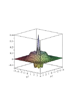
Figure 1: Winger function n=0

Figure 2: Winger function n=2

Figure 3: Winger function n=4

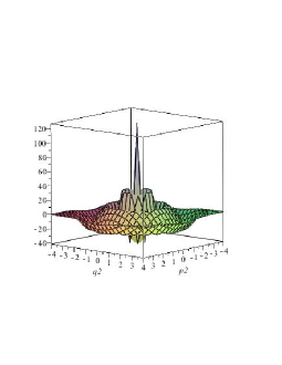
Figure 4: Winger function n=6

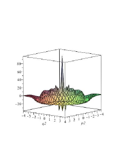
Figure 5: Winger function n=8

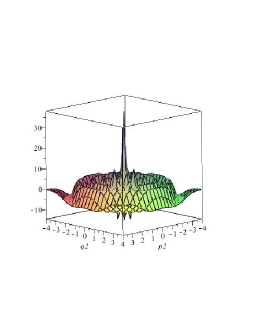
Figure 6: Winger function n=10

Table 1: Winger function n=0.

$\varepsilon$	Maximum	Minimum
0	0.082	-0.023
0.28	0.1	-0.03
0.5	0.162	-0.055
1	0.4	-0.151

Table 2: Winger function n=2.

$\varepsilon$	Maximum	Minimum
0	12.984	-4.803
0.28	13.187	-4.869
0.5	13.63	-5.013
1	15.57	-5.644

Table 3: Winger function n=4.

$\varepsilon$	Maximum	Minimum
0	69.986	-25.131
0.28	70.402	-25.233
0.5	71.313	-25.458
1	75.291	-26.438

Table 4: Winger function n=6.

$\varepsilon$	Maximum	Minimum
0	118.512	-39.587
0.28	119.153	-39.741
0.5	120.556	-40.078
1	126.689	-41.551

Table 5: Winger function n=8.

$\varepsilon$	Maximum	Minimum
0	91.654	-35.752
0.28	92.192	-35.948
0.5	93.368	-36.375
1	98.51	-38.244

Table 6: Winger function n=10.

$\varepsilon$	Maximum	Minimum
0	35	-13.229
0.28	35.235	-13.323
0.5	35.751	-13.529
1	38.002	-14.427

V.2 Second order correction

To establish second order corrections we make use of Eq.((31)). In order to obtain these corrections in terms of

$$(\widehat{H}^{0}(q,p)-E_{n}^{0})\psi_{n}^{2}=-(\widehat{V}-E_{n}^{1})\psi_{n}^{1}+E_{n}^{2}\psi_{n}^{0}\,,$$ (38)

which means

$$\psi_{n}^{1}=\sum_{m\neq n}a_{m}^{1}\psi_{m}^{0}$$ (39)

and

$$\psi_{n}^{2}=\sum_{m\neq n}a_{m}^{2}\psi_{m}^{0}\,.$$ (40)

If we use such dependencies into equation (38) then we have

$$\sum_{m\neq n}(E_{m}^{0}-E_{n}^{0})a_{m}^{2}\psi_{m}^{0} = -\sum_{m\neq n}\Big{[}(\widehat{V}-E_{n}^{1})a_{m}^{1}\psi_{m}^{0}$$

$$+ E_{n}^{2}\psi_{n}^{0}\Big{]}\,,$$

now we multiply the entire equation by $\psi_{k}^{{\dagger}\,0}(q,p)$ and integrate in $dpdq$, thus it yields

$$\sum_{k\neq n}a_{k}^{2}(E_{k}^{0}-E_{n}^{0}) = -\sum_{m\neq n}a_{m}^{1}\int\psi_{k}^{{\dagger}\,0}\widehat{V}\psi_{m}^{0}dpdq$$

$$+ \sum_{k\neq n}a_{k}^{1}E_{n}^{1}+E_{n}^{2}\delta_{kn}\,.$$

As before there are two possible cases, the first condition $k=n$ implies

$$E_{n}^{2}=\sum_{m\neq n}a_{m}^{1}\int\psi_{n}^{{\dagger}\,0}\widehat{V}\psi_{m}^{0}dpdq-a_{n}^{1}E_{n}^{1}$$

If we set $a_{n}^{1}=0$ in the previous equation, then we have

$$E_{n}^{2} = \sum_{m\neq n}a_{m}^{1}\int\psi_{n}^{{\dagger}\,0}\widehat{V}\psi_{m}^{0}dpdq$$ (42)

$$= \sum_{m\neq n}\frac{\int\psi_{m}^{{\dagger}\,0}\widehat{V}\psi_{n}^{0}}{E_{n}^{0}-E_{m}^{0}}dpdq\int\psi_{n}^{{\dagger}\,0}\widehat{V}\psi_{m}^{0}dpdq$$

$$= \sum_{m\neq n}\frac{|\int\psi_{m}^{{\dagger}\,0}\widehat{V}\psi_{n}^{0}|^{2}}{E_{n}^{0}-E_{m}^{0}}dpdq\,.$$

The equation (42) is the second order correction to the energy of the unperturbed system.

The second condition $k\neq n$ leads to

$$a_{m}^{2} = \sum_{k\neq n}\int\frac{\psi_{m}^{{\dagger}\,0}\widehat{V}\psi_{k}^{0}}{(E_{n}^{0}-E_{m}^{0})}dpdq\int\frac{\psi_{k}^{{\dagger}\,0}\widehat{V}\psi_{n}^{0}}{E_{n}^{0}-E_{k}^{0}}dpdq$$

$$- \int\frac{\psi_{m}^{{\dagger}\,0}\widehat{V}\psi_{n}^{0}}{(E_{n}^{0}-E_{m}^{0})^{2}}dpdq\int\psi_{n}^{{\dagger}\,0}\widehat{V}\psi_{n}^{0}\,,dpdq$$

therefore

$$\psi_{n}^{2} = \sum_{m\neq n}a_{m}^{2}\psi_{m}^{0}$$

$$= \sum_{m\neq n}\bigg{(}\sum_{k\neq n}\int\frac{\psi_{m}^{{\dagger}\,0}\widehat{V}\psi_{k}^{0}}{(E_{n}^{0}-E_{m}^{0})}dpdq\int\frac{\psi_{k}^{{\dagger}\,0}\widehat{V}\psi_{n}^{0}}{E_{n}^{0}-E_{k}^{0}}dpdq$$

$$- \int\frac{\psi_{m}^{{\dagger}\,0}\widehat{V}\psi_{n}^{0}}{(E_{n}^{0}-E_{m}^{0})^{2}}dpdq\int\psi_{n}^{{\dagger}\,0}\widehat{V}\psi_{n}^{0}dpdq\bigg{)}\psi_{m}^{0}$$

As a consequence the second order Wigner function is given by

$$f_{n}^{2}(q_{x},p_{x},q_{y},p_{y})=\psi_{n_{x}}(q_{x},p_{x})\psi_{n_{y}}(q_{y},p_{y})\ast\psi_{n_{x}}^{\dagger}(q_{x},p_{x})\psi_{n_{y}}^{\dagger}(q_{y},p_{y})\,,$$

the results for some cases are presented in figures FIG.7, FIG.8, FIG.9, FIG.10 and FIG.11. We also chart some results on tables TABLE 7, TABLE 8, TABLE 9, TABLE 10 and TABLE 11.

Figure 7: Winger function second order n=0

Figure 8: Winger function second order n=2

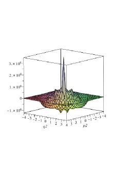
Figure 9: Winger function second order n=4

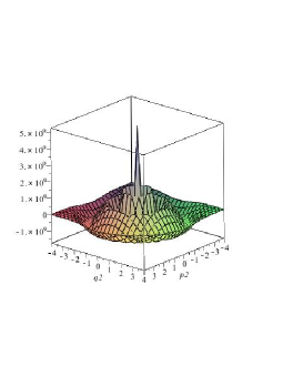
Figure 10: Winger function second order n=6

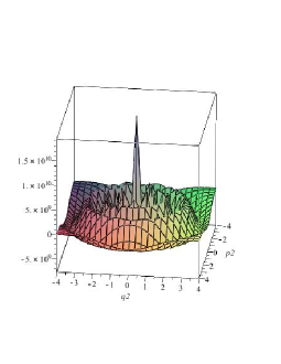
Figure 11: Winger function second order n=8

Table 7: Winger function second order n=0.

$\varepsilon$	Maximum	Minimum
0	6.165	-2.555
0.28	6.518	-2.599
0.5	7.334	-2.708
1	11.63	-3.995

Table 8: Winger function second order n=2.

$\varepsilon$	Maximum	Minimum
0	$3.214131\times 10^{6}$	-847282.769
0.28	$3.221852\times 10^{6}$	-847109.82
0.5	$3.238755\times 10^{6}$	-846731.218
1	$3.312671\times 10^{6}$	-845075.61

Table 9: Winger function second order n=4.

$\varepsilon$	Maximum	Minimum
0	$3.41392\times 10^{8}$	$-1.23009\times 10^{8}$
0.28	$3.419019\times 10^{8}$	$-1.231347\times 10^{8}$
0.5	$3.43018\times 10^{8}$	$-1.234099\times 10^{8}$
1	$3.47896\times 10^{8}$	$-1.246125\times 10^{8}$

Table 10: Winger function second order n=6.

$\varepsilon$	Maximum	Minimum
0	$5.177845\times 10^{9}$	$-1.736374\times 10^{9}$
0.28	$5.18489\times 10^{9}$	$-1.738067\times 10^{9}$
0.5	$5.200312\times 10^{9}$	$-1.741771\times 10^{9}$
1	$5.267715\times 10^{1}0$	$-1.757962\times 10^{9}$

Table 11: Winger function second order n=8.

$\varepsilon$	Maximum	Minimum
0	$1.910526\times 10^{1}0$	$-7.538693\times 10^{9}$
0.28	$1.913466\times 10^{1}0$	$-7.549376\times 10^{9}$
0.5	$1.919899\times 10^{1}0$	$-7.572756\times 10^{9}$
1	$1.948017\times 10^{1}0$	$-7.674945\times 10^{9}$

VI The non-classicality indicator

The volume of negative part of Wigner function can be interpreted as a signature of quantum interference. In this way, a measure of non-classicality of quantum states is defined by negativity indicator, which is given by nc

$$\eta(\psi) = \int\int\left[|f_{W}\,{}_{\psi}(q,p)|-F_{W}\,{}_{\psi}(q,p)\right]dpdq$$

$$= \int\int|F_{W}\,{}_{\psi}(q,p)|dpdq-1.$$

This indicator represents the doubled volume of the integrated part of the Wigner function. In sequence, we calculated numerically this indicator for one dimensional hydrogen atom. The results of this calculation are shown in Table 12 below. A interesting result is that the parameter $\eta(\psi)$ for $n=1$, the fundamental level of hydrogen atom, is equals to zero. This point shows that in this level the hydrogen atom can be studied by classical mechanics methods.

Table 12: One-dimensional Hydrogen atom.

$n$	$\eta(\psi)$
1	0
2	0.416375
3	0.693456
4	0.956789
5	1.217456
6	1.334907
7	1.491342
8	1.778512
9	1.901238

In addition, we calculate numerically the non-classicality indicator for hydrogen atom with Henon-Heiles interaction. The results are shown in Tables TABLE 13, TABLE 14, TABLE 15 and TABLE 16. An interesting result is the fact that the negativity indicator grows in the same direction of interaction parameter $\epsilon$. This latter result implies that the quantum entanglement of quantum system analyzed increases when the indicator parameter grows. It is important for quantum computing qc1 , for example.

Table 13: Negativity parameter for $\epsilon=0$.

$n$	$\eta(\psi)$
0	0
2	0.32645
4	0.45786
6	0.53647
8	0.60185

Table 14: Negativity parameter for $\epsilon=0.28$.

$n$	$\eta(\psi)$
0	0.16783
2	0.35784
4	0.46210
6	0.54678
8	0.63193

Table 15: Negativity parameter for $\epsilon=0.5$.

$n$	$\eta(\psi)$
0	0.19773
2	0.38954
4	0.47841
6	0.56823
8	0.67918

Table 16: Negativity parameter for $\epsilon=1$.

$n$	$\eta(\psi)$
0	0.20376
2	0.39932
4	0.50385
6	0.58762
8	0.72431

VII Concluding remarks

The present work deals with the problem of constructing a formalism in phase space based on the unitary symmetry. We have used the algebraic structure of the Wigner function, along with the notion of star-products, to construct unitary representations for the Galilei group. Then the physical aspects of the formalism are discussed and, in particular, the physical meaning of a quantum state is obtained by introducing the notion of quasi-amplitudes of probability in $\Gamma$, which is related to the Wigner quasi-probability. The Schrödinger equation is constructed in phase space and as an application, the Wigner function for the Hydrogen is derived. Then we add a Hénon-Heiles potential to the Hamiltonian of the Hydrogen atom and calculate corrections of Wigner function at first and second order of pertubation. We presented our results in the panels and tables along the article.

Appendix A Calculation of $a_{n}$

In this appendix we present the coefficients $a_{n}$.

$$a0 = \sqrt{n_{x}(n_{x}-1)}\psi_{n_{x}-2}^{(0)}\sqrt{n_{y}}\psi_{n_{y}-1}^{(0)}-\sqrt{n_{x}(n_{x}-1)}\psi_{n_{x}-2}^{(0)}\sqrt{n_{y}+1}\psi_{n_{y}+1}^{(0)}$$

$$- \sqrt{(n_{x}+1)(n_{x}+2)}\psi_{n_{x}+2}^{(0)}\sqrt{n_{y}}\psi_{n_{y}-1}^{(0)}+\sqrt{(n_{x}+1)(n_{x}+2)}\psi_{n_{x}+2}^{(0)}\sqrt{n_{y}+1}\psi_{n_{y}+1}^{(0)}\,,$$

$$a1 = \frac{1}{3}\sqrt{n_{y}(n_{y}-1)(n_{y}-2)}\psi_{n_{y}-3}^{(0)}+\bigg{(}\sqrt{n_{y}(n_{y}+1)^{2}}+\sqrt{n_{y}^{3}}+\sqrt{n_{y}(n_{y}-1)^{2}}\bigg{)}\psi_{n_{y}-1}^{(0)}$$

$$- \bigg{(}\sqrt{(n_{y}+1)(n_{y}+2)^{2}}+\sqrt{(n_{y}+1)^{3}}+\sqrt{n_{y}^{2}(n_{y}+1)}\bigg{)}\psi_{n_{y}+1}^{(0)}$$

$$- \frac{1}{3}\sqrt{(n_{y}+1)(n_{y}+2)(n_{y}+3)}\psi_{n_{y}+3}^{(0)}\,,$$

$$a2 = \bigg{(}\frac{1}{8}\sqrt{n_{x}(n_{x}-1)(n_{x}-2)(n_{x}-3)}\psi_{n_{x}-4}^{(0)}+\frac{1}{4}\sqrt{n_{x}(n_{x}+1)^{2}(n_{x}-1)}\psi_{n_{x}-2}^{(0)}$$

$$+ \frac{1}{4}\sqrt{n_{x}^{3}(n_{x}+1)}\psi_{n_{x}-2}^{(0)}\bigg{)}\sqrt{n_{y}(n_{y}-1)}\psi_{n_{y}-2}^{(0)}$$

$$+ \sqrt{n_{x}(n_{x}-1)}\psi_{n_{x}-2}^{(0)}\bigg{(}\frac{1}{8}\sqrt{n_{y}(n_{y}-1)(n_{y}-2)(n_{y}-3)}\psi_{n_{y}-4}^{(0)}$$

$$+ \frac{1}{4}\sqrt{n_{y}(n_{y}+1)^{2}(n_{y}-1)}\psi_{n_{y}-2}^{(0)}+\frac{1}{4}\sqrt{n_{y}^{3}(n_{y}-1)}\psi_{n_{y}-2}^{(0)}\bigg{)}\,,$$

$$a3 = \sqrt{n_{x}(n_{x}-1)}\psi_{n_{x}-2}^{(0)}\bigg{(}\frac{1}{4}\sqrt{n_{y}(n_{y}-1)^{3}}\psi_{n_{y}-2}^{(0)}-\frac{1}{4}\sqrt{(n_{y}+1)(n_{y}+2)(n_{y}+3)^{2}}\psi_{n_{y}+2}^{(0)}$$

$$+ \frac{1}{4}\sqrt{n_{y}(n_{y}-1)(n_{y}-2)^{2}}\psi_{n_{y}-2}^{(0)}-\frac{1}{4}\sqrt{(n_{y}+1)(n_{y}+2)^{3}}\psi_{n_{y}-2}^{(0)}\bigg{)}$$

$$+ \bigg{(}-\frac{1}{8}\sqrt{n_{x}(n_{x}-1)(n_{x}-2)(n_{x}-3)}\psi_{n_{x}-4}^{(0)}-\frac{1}{4}\sqrt{n_{x}(n_{x}-1)(n_{x}+2)^{2}}\psi_{n_{x}-2}^{(0)}$$

$$- \frac{1}{4}\sqrt{n_{x}^{3}(n_{x}-1)}\psi_{n_{x}-2}^{(0)}\bigg{)}\sqrt{(n_{y}+1)+(n_{y}+2)}\psi_{n_{y}+2}^{(0)}$$

$$+ \sqrt{n_{x}(n_{x}-1)}\psi_{n_{x}-2}^{(0)}\bigg{(}-\frac{1}{4}\sqrt{(n_{y}+1)^{3}(n_{y}+2)}\psi_{n_{y}+2}^{(0)}-\frac{1}{4}\sqrt{n_{y}^{2}(n_{y}+1)(n_{y}+2)}\psi_{n_{y}+2}^{(0)}$$

$$- \frac{1}{8}\sqrt{(n_{y}+1)(n_{y}+2)(n_{y}+3)(n_{y}+4)}\psi_{n_{y}+4}^{(0)}\bigg{)}\,,$$

$$a4 = \bigg{(}\frac{1}{4}\sqrt{n_{x}(n_{x}-1)^{3}}\psi_{n_{x}-2}^{(0)}-\frac{1}{4}\sqrt{(n_{x}+1)(n_{x}+2)(n_{x}+3)^{2}}\psi_{n_{x}+2}^{(0)}\bigg{)}\sqrt{n_{y}(n_{y}-1)}\psi_{n_{y}-2}^{(0)}$$

$$+ \bigg{(}-\frac{1}{4}\sqrt{n_{x}(n_{x}-1)^{3}}\psi_{n_{x}-2}^{(0)}+\frac{1}{4}\sqrt{(n_{x}+1)(n_{x}+2)(n_{x}+3)^{2}}\psi_{n_{x}+2}^{(0)}\bigg{)}\sqrt{(n_{y}+1)(n_{y}+2)}\psi_{n_{y}+2}^{(0)}$$

$$+ \bigg{(}\frac{1}{4}\sqrt{n_{x}(n_{x}-1)(n_{x}-2)^{2}}\psi_{n_{x}-2}^{(0)}-\frac{1}{4}\sqrt{(n_{x}+1)(n_{x}+2)^{3}}\psi_{n_{x}+2}^{(0)}\bigg{)}\sqrt{n_{y}(n_{y}-1)}\psi_{n_{x}-2}^{(0)}$$

$$+ \bigg{(}-\frac{1}{4}\sqrt{n_{x}(n_{x}-1)(n_{x}-2)^{2}}\psi_{n_{x}-2}^{(0)}+\frac{1}{4}\sqrt{(n_{x}+1)(n_{x}+2)^{3}}\psi_{n_{x}+2}^{(0)}\bigg{)}\sqrt{(n_{y}+1)(n_{y}+2)}\psi_{n_{y}+2}^{(0)}$$

$$+ \bigg{(}-\frac{1}{4}\sqrt{(n_{x}+1)^{3}(n_{x}+2)}\psi_{n_{x}+2}^{(0)}-\frac{1}{4}\sqrt{n_{x}^{2}(n_{x}+1)(n_{x}+2)}\psi_{n_{x}+2}^{(0)}$$

$$- \frac{1}{8}\sqrt{(n_{x}+1)(n_{x}+2)(n_{x}+3)(n_{x}+4)}\psi_{n_{x}+4}^{(0)}\bigg{)}\sqrt{n_{y}(n_{y}-1)}\psi_{n_{x}-2}^{(0)}\,,$$

$$a5 = \sqrt{(n_{x}+1)(n_{x}+2)}\psi_{n_{x}+2}^{(0)}\bigg{(}-\frac{1}{8}\sqrt{n_{y}(n_{y}-1)(n_{y}-2)(n_{y}-3)}\psi_{n_{y}-4}^{(0)}$$

$$- \frac{1}{4}\sqrt{n_{y}(n_{y}-1)(n_{y}+1)^{2}}\psi_{n_{y}-2}^{(0)}-\frac{1}{4}\sqrt{n_{y}^{3}(n_{y}-1)}\psi_{n_{y}-2}^{(0)}-\frac{1}{4}\sqrt{n_{y}(n_{y}-1)^{3}}\psi_{n_{y}-2}^{(0)}$$

$$+ \frac{1}{4}\sqrt{(n_{y}+1)(n_{y}+2)(n_{y}+3)^{2}}\psi_{n_{y}+2}^{(0)}-\frac{1}{4}\sqrt{n_{y}(n_{y}-1)(n_{y}-2)^{2}}\psi_{n_{y}-2}^{(0)}$$

$$+ \frac{1}{4}\sqrt{(n_{y}+1)(n_{y}+2)^{3}}\psi_{n_{y}+2}^{(0)}\bigg{)}\,,$$

$$a6 = \bigg{(}\frac{1}{4}\sqrt{(n_{x}+1)^{3}(n_{x}+2)}\psi_{n_{x}+2}^{(0)}+\frac{1}{4}\sqrt{n_{x}^{2}(n_{x}+1)(n_{x}+2)}\psi_{n_{x}+2}^{(0)}$$

$$+ \frac{1}{8}\sqrt{(n_{x}+1)(n_{x}+2)(n_{x}+3)(n_{x}+4)}\psi_{n_{x}+4}^{(0)}\bigg{)}\sqrt{(n_{y}+1)(n_{y}+2)}\psi_{n_{y}+2}^{(0)}$$

$$+ \sqrt{(n_{x}+1)(n_{x}+2)}\psi_{n_{x}+2}^{(0)}\bigg{(}\frac{1}{4}\sqrt{(n_{y}+1)^{3}(n_{y}+2)}\psi_{n_{y}+2}^{(0)}$$

$$+ \frac{1}{4}\sqrt{n_{y}^{2}(n_{y}+1)(n_{y}+2)}\psi_{n_{y}+2}^{(0)}+\frac{1}{8}\sqrt{(n_{y}+1)(n_{y}+2)(n_{y}+3)(n_{y}+4)}\psi_{n_{y}+4}^{(0)}\bigg{)}$$

and

$$a7 = \bigg{(}\frac{1}{2}\sqrt{n_{x}(n_{x}-1)}\psi_{n_{x}-2}^{(0)}-\frac{1}{2}\sqrt{(n_{x}+1)(n_{x}+2)}\psi_{n_{x}+2}^{(0)}+\frac{1}{2}\sqrt{n_{y}(n_{y}-1)}\psi_{n_{y}-2}^{(0)}$$

$$- \frac{1}{2}\sqrt{(n_{y}+1)(n_{y}+2)}\psi_{n_{y}+2}^{(0)}\bigg{)}\,.$$

References

- (1) M. Hénon and C. Heiles, Astronomical Journal, 69, 73 (1964).
- (2) H. Friedrich and D. Wintgen, Phys. Rep. (Review Section of Physics Letters), 2, 37 (1939).
- (3) J. S. Hutchinson and R. E. Wyatt, Chem. Phys. Let., 72, 2, 378 (1980).
- (4) A. B. Adelsoye and A. o. Akala, Lat. Am. J. Phys. Educ., 4, 3, 598 (2010).
- (5) H.T.C. Stoof, M. Houbiers, C.A. Sackett and R.G. Hulet, Phys. Rev. Lett. 76, 10 (1996).
- (6) C.J. Myatt, E.A. Burt, R.W. Ghrist, E.A. Cornell and C.E. Wieman, Phys. Rev. Lett. 78, 586 (1997).
- (7) E. Hodby, S.T. Thompson, C.A. Regal, M. Greiner, A.C. Wilson, D.S. Jin, E.A. Cornell, C.E. Wieman, Phys. Rev. Lett. 94, 120402 (2005).
- (8) K.E. Strecker, G.B. Partridge and R.G. Hulet, Phys. Rev. Lett. 91, 080406 (2003).
- (9) J. Cubizolles, T. Bourdel, S.J.J.M.F. Kokkelmans, G.V. Shlyapnikov, and C. Salomon, Phys. Rev. Lett. 91, 240401 (2003).
- (10) T. Bourdel, L. Khaykovich, J. Cubizolles, J. Zhang, F. Chevy, M. Teichmann, L. Tarruell, S.J.J.M.F. Kokkelmans, and C. Salomon, Phys. Rev. Lett. 93, 050401 (2004).
- (11) A. Shimony, Measures of Entanglement, in The Dilemma of Einstein, Podolsky and Rosen – 60 Years Later, Edited by A. Mann and M. Revzen (IOP, Bristol, 1996).
- (12) G. Alber, T. Beth, M. Horodecki, P. Horodecki, R. Horodecki, M. Rötteler, H. Weinfurter, R. Werner, and A. Zeilinger, Quantum Information (Springer-Verlag, Berlin, 2001).
- (13) Y. Ohnuki and T. Kashiwa, Prog. Theor. Phys. 60, 548 (1978).
- (14) F. Hong-yi, Phys. Rev. A 40, 4237 (1989).
- (15) K. Svozil, Phys. Rev. Lett. 65, 3341 (1990).
- (16) S. Chaturvedi, R. Sandhya, V. Srinivasan and R. Simon, Phys. Rev. A 41, 3969 (1990).
- (17) K.E. Cahill and R.J. Glauber, Phys. Rev. A 59, 1538 (1999).
- (18) E.P. Wigner, Phys. Rev. 40, 749 (1932).
- (19) M. Hillery, R. F. O ’Connell, M. O. Scully, E. P. Wigner, Phys. Rep. 106, 121 (1984).
- (20) Y.S. Kim, M.E. Noz, Phase Space Picture and Quantum Mechanics - Group Theoretical Approach (W. Scientific, London, 1991).
- (21) T. Curtright, D. Fairlie, C. Zachos, Phys. Rev. D 58, 25002 (1998).
- (22) D. Galetti and A.F.R. de Toledo Piza, Physica A 214, 207 (1995).
- (23) L.G. Lutterbach and L. Davidovich, Phys. Rev. Lett. 78, 2547 (1997).
- (24) A.E. Santana, A. Matos Neto, J.D.M. Vianna and F.C. Khanna, Physica A 280, 405 (2000).
- (25) M.D. Oliveira, M.C.B. Fernandes, F.C. Khanna, A.E. Santana and J.D.M. Vianna, Ann. Phys. (N.Y.) 312, 492 (2004).
- (26) V.V. Dodonov, Phys. Lett. A 364, 368 (2007).
- (27) G. Torres-Vega, J.H. Frederick, J. Chem. Phys. 93, 8862 (1990).
- (28) G. Torres-Vega, J.H. Frederick, J. Chem. Phys. 98, 3103 (1993).
- (29) B.O. Koopman, Proc. Natl. Acad. Sci. (USA) 17, 315 (1931).
- (30) M. Schönberg, N. Cimento, 9, 1139 (1952);
- (31) M. Schönberg, N. Cimento, 10, 419 (1953).
- (32) M. Schönberg, N. Cimento, 10, 697 (1953).
- (33) A. Loinger , Ann. Phys. (N.Y.) 20, 132 (1962).
- (34) G. Lugarini and M. Pauri, Ann. Phys. (N.Y.) 44, 226 (1967).
- (35) J.-M. Lévy-Leblond, F. Lurçat, J. Math. Phys. 6, 1564 (1965).
- (36) M.C.B. Fernandes e J.D.M. Vianna, Found. Phys. 29, 201 (1999).
- (37) L.M. Abreu, A.E. Santana and A. Ribeiro-Filho, Ann. Phys. (NY) 297, 396 (2002).
- (38) F. C. Khanna, A. P. C. Malbouisson, J. M. C. Malbouisson, A. E. Santana, Thermal Quantum Field Theory: Algebraic Aspects and Applications (W. Scientific, Singapore, 2009).
- (39) H. Weyl, Z. Phys. 46, 1 (1927).
- (40) J.E. Moyal, Proc. Camb. Phil. Soc. 45, 99 (1949).
- (41) R.G.G. Amorim, M.C.B. Fernandes, F.C. Khanna, A.E. Santana, J.D.M. Vianna, Phys. Lett. A 361, 464 (2007).
- (42) S.A. Smolyansky, A.V. Prozorkevich, G. Maino, S.G. Mashnic, Ann. Phys. (N.Y.) 277, 193 (1999).
- (43) I. Galaviz, H. García-Compeán, M. Przanowski, F.J. Turrubiates, Weyl-Wigner-Moyal for Fermi Classical Systems, arXiv: hep-th/0612245v1.
- (44) J. Dito, J. Math. Phys. 33, 791 (1992).
- (45) R.G.G. Amorim, F.C. Khanna, A.E. Santana, J.D.M. Vianna, Physica A 388, 3771 (2009).
- (46) M.C.B. Fernandes, F.C. Khanna, M.G.R. Martins, A.E. Santana, J.D.M. Vianna, Physica A, 389 , 3409 (2010).
- (47) L.M. Abreu, A.E. Santana, A. Ribeiro Filho, Ann. Phys. (N.Y.) 297, 396 (2002).
- (48) M.C.B. Fernandes, J.D.M. Vianna, Braz. J. Phys. 28, 2 (1999).
- (49) M.C.B. Fernandes, A. E. Santana, J. D. M. Vianna, J. Phys. A: Math. Gen. 36, 3841 (2003).
- (50) A.E. Santana, A. Matos Neto, J.D.M. Vianna, F.C. Khanna, Physica A 280, 405 (2001).
- (51) D. Bohm, B.J. Hiley, Found. Phys. 11, 179 (1981).
- (52) M.C.B. Andrade, A.E. Santana, J.D.M. Vianna, J. Phys. A: Math. Gen. 33, 4015 (2000).
- (53) M.A. Alonso, G.S. Pogosyan, K.B. Wolf, J. Math. Phys. 43, 5857 (2002).
- (54) R.G.G. Amorim, M.C.B. Fernandes, F.C. Khanna, A.E. Santana, J.D.M. Vianna, Int. J. Mod. Phys. A 28, 1350013 (2013)
- (55) R.G.G. Amorim, S.C. Ulhoa, A.E. Santana, Braz. J. Phys. 43, 78 (2013).
- (56) M.A. de Gosson, Bull. Sci. Math. 121, 301 (1997).
- (57) M.A. de Gosson, Ann. Inst. H Poincaré 70, 547 (1999).
- (58) M.A. de Gosson, J. Phys. A: Math. Gen. 37, 7297 (2004).
- (59) M.A. de Gosson, Lett. Math. Phys. 72, 293 (2005).
- (60) M. Blaszak, Z. Domanky, Ann. Phys. 327, 167 (2012).
- (61) A.L. Fetter and J. D. Walecka, Quantum Theory of Many-Particles Systems (McGraw-Hill, N. York, 1971).
- (62) L.K. Haines, D.H. Roberts, Am. J. Phys. 37, 1145 (1939).
- (63) A.N. Gordeyev, S.C. Chhajlany, J. Phys. A: Math. Gen. 30, 6893 (1997).
- (64) Q.S. Li, J. Lu, Chem. Phys. Lett. 336, 118 (2001).
- (65) N.R. Kestner, J. Chem. Phys. 45, 213 (1995).
- (66) N.R. Kestner, O Sinanoglu, Phys. Rev., 2687 (1962).
- (67) D.P. O’Neil, P.M.W. Gill, Phys. Rev. A 68, 022505 (2003).
- (68) A. Kenfack, K. Zyczkowski, J. Opt. B: Quantum Semiclass. Opt. 6, 396 (2004).
- (69) V. Veitch, C. Ferrie, D. Gross, J. Emerson, New J. Physics 15, 0039502 (2013).