A spin glass approach to the directed feedback vertex set problem

Abstract

A directed graph (digraph) is formed by vertices and arcs (directed edges) from one vertex to another. A feedback vertex set (FVS) is a set of vertices that contains at least one vertex of every directed cycle in this digraph. The directed feedback vertex set problem aims at constructing a FVS of minimum cardinality. This is a fundamental cycle-constrained hard combinatorial optimization problem with wide practical applications. In this paper we construct a spin glass model for the directed FVS problem by converting the global cycle constraints into local arc constraints, and study this model through the replica-symmetric (RS) mean field theory of statistical physics. We then implement a belief propagation-guided decimation (BPD) algorithm for single digraph instances. The BPD algorithm slightly outperforms the simulated annealing algorithm on large random graph instances. The predictions of the RS mean field theory are noticeably lower than the BPD results, possibly due to its neglect of cycle-caused long range correlations.

• Janary 17, 2016 (first version); April 04, 2016 (revised version)

1 Introduction

Directed graphs (digraphs) are widely used to describe interactions in technological, biological, and social complex systems [1, 2, 3]. A digraph is composed of vertices and arcs (directed edges) which link between vertices. For instance, the gene regulation system of a biological cell can be modeled as a digraph of genes, in which an arc points from gene $A$ to gene $B$ if $A$ regulates the expression of $B$ [4, 5]. Real-world complex systems are full of feedback interactions and adaptation mechanisms, and the digraphs of these systems usually contain an abundant number of directed cycles, which make the system’s dynamical properties difficult to predict and to externally control [6, 7].

Not all vertices and arcs are equally important in feedback interactions. Some vertices and arcs may participate in a much greater number of directed cycles than other vertices and arcs. A minimum feedback vertex set (FVS) contains a smallest number of vertices whose deletion from the digraph destroys all the directed cycles. Similarly, a minimum feedback arc set (FAS) is an arc set of smallest cardinality such that every directed cycle of the digraph has at least one arc in this set. In terms of collective effect, the vertices in a FVS and the arcs in a FAS may be most significant to the dynamical complexity of a complex networked system [8, 9, 10], and these vertices and arcs may also be optimal targets of distributed network attack processes [11, 12].

The directed feedback problems, namely constructing a minimum FVS and a minimum FAS for a generic digraph, are combinatorial optimization problems in the nondeterministic polynomial-hard (NP-hard) class and therefore are intrinsically very difficult [13]. Some progresses have been achieved by computer scientists and applied mathematicians in understanding this classic hard problem since the 1990s [10]. Approximate algorithms with provable bounds have been designed (see, for example [14, 15, 16]) and efficient heuristic algorithms such as greedy local search [17] and simulated annealing [18] have been implemented and tested on benchmark small problem instances. Yet unlike the FVS problem on an undirected graph [19, 20], it is still very difficult to give tight bounds on the minimal cardinality of the directed FVS and FAS problems.

In this paper we study the directed FVS problem using statistical physics methods. Our method is also applicable to the FAS problem since it is essentially equivalent to the FVS problem [14]. We construct a spin glass model for the directed FVS problem and derive the replica-symmetric (RS) mean field theory for this model. The mean field theory enables us to estimate the minimum directed FVS cardinality for random digraphs. Based on this mean field theory we implement a belief propagation-guided decimation (BPD) algorithm and apply this message-passing algorithm to large random digraph instances. The BPD algorithm slightly outperforms the simulated annealing algorithm [18] in terms of the FVS cardinality and the arc density of the remaining directed acyclic graph (DAG), while the computing times of the two algorithms are comparable to each other. Our work will be helpful for future investigations on the dynamical complexity of various real-world networked systems and for further studies of targeted attacks on directed networks. In this paper we also point out a major difficulty of the RS mean field theory in treating directed cycle-caused long range correlations.

Directed and undirected cycles cause long-range correlations and frustrations in dynamical systems and spin glass models. They are very important network structural properties, but theoretical efforts directly treating them as constraints are quite lacking. Directed cycles are global properties of a digraph (each of which may involve a lot of vertices and arcs). Compared with problems with local constraints (such as the $K$-satisfiability problem [21, 22, 23]), optimization problems constrained by directed cycles are much more difficult to tackle theoretically. The present paper is a continuation of our earlier report [24] which treated the undirected FVS problem successfully. We realized that the directness of the cycle constraints makes the directed FVS problem much harder than its undirected counterpart. It is clear that further efforts are needed to overcome the gap between the BPD results and the RS predictions in Fig. 6.

The next section defines the directed FVS and FAS problems and explains their essential equivalence. We then introduce a FVS spin glass model in Sec. 3 and study it by RS mean field theory in Sec. 4. In Sec. 5 we describe the BPD message-passing algorithm and compare its performance with the simulated annealing algorithm on random digraphs. We conclude this paper in Sec. 6. The two appendices contain some additional technical discussions.

2 The directed FVS and FAS problems

Consider a simple digraph $G$. This digraph contains $N$ vertices whose indices (say $i,j,k,\ldots$) range from integer values $1$ to $N$. There are $M$ arcs in this digraph, each of which points from one vertex (say $i$) to another different vertex (say $j$) and is denoted as $[i,j]$. There is no self-arc pointing from a vertex to itself, and there is at most one arc from any vertex $i$ to any another different vertex $j$. The arc density $\alpha$ of a digraph is just the ratio between arc number $M$ and vertex number $N$, that is $\alpha\equiv\frac{M}{N}$.

Each vertex $i$ of the digraph has a positive weight $w_{i}$ whose meaning is context-dependent. For instance, in the problem of complex-system control [7], the weight $w_{i}$ may be the cost of monitoring the vertex $i$. The vertex weights are fixed parameters of the digraph and can not be modified. In the actual numerical computations of this paper, each vertex weight $w_{i}$ is set to be $w_{i}=1$ just for simplicity.

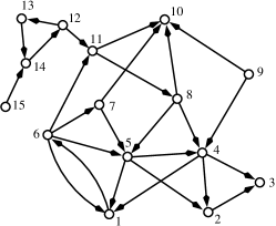
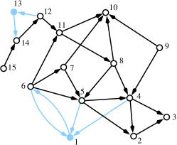
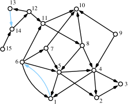
Figure 1: (a) A small digraph containing $N=15$ vertices and $M=25$ arcs, (b) a minimum feedback vertex set $\{1,13\}$ and (c) a minimum feedback arc set $\{[1,6],[13,14]\}$ for this digraph.

If there is an arc $[i,j]$ from a vertex $i$ to another vertex $j$ but the reverse arc $[j,i]$ is absent, then $j$ is said to be a child of $i$ and $i$ is said to be a parent of $j$. If there are two arcs $[i,j]$ and $[j,i]$ of reverse direction between vertices $i$ and $j$, then vertex $i$ is said to be a brother of vertex $j$ and $j$ a brother of $i$. The in-degree and out-degree of vertex $j$ are defined as the total number of arcs pointing to $j$ and pointing from $j$, respectively. For example, vertex $5$ in Fig. 1 is a parent of vertex $1$ and is a child of vertex $6$, while vertices $6$ and $1$ are brother of each other.

A directed path in a digraph $G$ is a sequence of arcs which connect a sequence of vertices, for example a directed path $[i,j_{1}],\ [j_{1},j_{2}],\ \ldots,\ [j_{n-1},j_{n}],\ [j_{n},j]$ from a start vertex $i$ to an end vertex $j$. If the start vertex and the end vertex of a directed path are identical, then this path is referred to as a directed cycle. Some examples of directed paths and cycles can be found in the small graph of Fig. 1.

A feedback vertex set of digraph $G$ is a subset $\Gamma$ of the $N$ vertices such that if all the vertices of this set and the attached arcs are removed from $G$ the remaining digraph will have no directed cycle. In other words, the set $\Gamma$ contains at least one vertex of every directed cycle. As an example, the set $\Gamma=\{1,13\}$ is a FVS for the small digraph of Fig. 1. Similarly, a feedback arc set is a subset of the $M$ arcs such that it contains at least one arc of every directed cycle of digraph $G$. For the example of Fig. 1 one can easily verify that the arc set $\{[1,6],[13,14]\}$ is a minimum FAS.

The weight $w(\Gamma)$ of a feedback vertex set $\Gamma$ is just the total weight of its ingredient vertices: $w(\Gamma)\equiv\sum_{i\in\Gamma}w_{i}$. The fundamental goal of the feedback vertex set problem is to construct a FVS for a given digraph with total weight as small as possible. This NP-hard problem has been studied by mathematicians and computer scientists, see for example references [10, 14, 15, 16, 17, 18], but it appears that this important problem has not yet been treated by statistical physics methods. Here we work on the directed FVS problem using the mean field spin glass theory and the belief propagation message-passing algorithm.

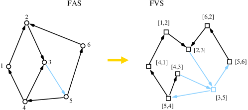
Figure 2: The feedback arc set problem for a digraph $G$ (left) can be converted into a feedback vertex set problem for a new digraph $\tilde{G}$ (right). Each arc $[i,j]$ of $G$ is mapped to a vertex (denoted by a square) in $\tilde{G}$, and an arc is created in $\tilde{G}$ from a vertex $[i,j]$ to another vertex $[k,l]$ if and only if $j=k$. The left digraph becomes acyclic after arc $[3,5]$ is deleted, and correspondingly the right digraph becomes acyclic after vertex $[3,5]$ and its attached arcs are deleted.

The spin glass model of this work and the corresponding BPD algorithm is also applicable to the FAS problem. This is because the FAS problem is equivalent to the FVS problem on a modified digraph [14] (Fig. 2). To construct a FAS for a given digraph $G$, we can first map each arc $[i,j]$ of $G$ to a vertex (also denoted as $[i,j]$) of a new digraph $\tilde{G}$, and then we setup an arc in $\tilde{G}$ from a vertex $[i,j]$ to another vertex $[k,l]$ if and only if $j=k$. It is easy to verify that there is a one-to-one correspondence between a directed cycle of digraph $G$ and a directed cycle in the digraph $\tilde{G}$, and a FVS of digraph $\tilde{G}$ is just a FAS of digraph $G$ (Fig. 2).

In the present paper we focus on the directed FVS problem. Treatment of the FAS problem on random and real-world networks and its application to the network destruction problem will be reported in a separate paper [25].

3 Spin glass model

We now describe in detail a spin glass model for the directed FVS problem, which was briefly introduced in the last section of [24] by the present author. Similar model systems have also been discussed by other authors, see, e.g., [27, 28, 29]. First, a height state $h_{i}$ is assigned to each vertex $i$ of a digraph $G$. This height state can take integer values in the interval $0\leq h_{i}\leq D$, with $D$ being the allowed maximal height in the model. The value of $D$ is adjustable in the theoretical calculations, but it should not exceed the total number $N$ of vertices. Setting $D$ to a larger value will result in better theoretical results. On the other hand, the memory space and the computing time both increase linearly with $D$. In this paper we mainly work with $D=200$ but we will also discuss the effect of $D$ on the theoretical results.

A generic configuration of the system is denoted as $\underline{h}$ with $\underline{h}\equiv\{h_{1},h_{2},\ldots,h_{N}\}$. If the height of a vertex $i$ is $h_{i}=0$, this vertex is referred to as being unoccupied or empty, otherwise $i$ is referred to as being occupied. To ensure that there are no directed cycles within the set of occupied vertices, we impose the following constraint on each arc $[i,j]$ of digraph $G$: if both vertex $i$ and vertex $j$ are occupied ($h_{i}>0$ and $h_{j}>0$), then the height of vertex $i$ must be less than that of vertex $j$ ($h_{i}<h_{j}$). A configuration $\underline{h}$ is referred to as a legal configuration if it satisfies all the $M$ arc constraints.

If $\underline{h}$ is a legal configuration of digraph $G$, then the vertex heights along any directed path of occupied vertices form a strictly increasing sequence. Therefore there must be no directed cycles within the set of occupied vertices of configuration $\underline{h}$ and the set of unoccupied vertices of this configuration must form a FVS. In other words, each legal configuration $\underline{h}$ corresponds to exactly one FVS.

On the other hand, since two or more legal configurations may have the identical set of unoccupied vertices, a single FVS often corresponds to more than one legal configuration. In this sense the above introduced arc constraints are not very restrictive. We can achieve a one-to-one mapping between a legal configuration and a FVS by requiring that if the height of a vertex is positive it must exceed the maximal height of its parent and brother vertices by $1$ (see A). But the spin glass model with such a set of more restrictive arc constraints is more complicate for numerical treatment, and it does not lead to better FVS solutions for single digraph instances. In the present paper we stick to the weaker arc constraints. A comparative study on this weaker model and the stronger model of A will be carried out in another technical paper.

For the convenience of theoretical development, if there is an arc $[i,j]$ between a vertex $i$ and another vertex $j$ but the reverse arc $[j,i]$ is absent, we denote this situation by the notation $(i\rightarrow j)$; if both the forward arc $[i,j]$ and the reverse arc $[j,i]$ exist between vertices $i$ and $j$, we denote this situation by the notation $(i\Leftrightarrow j)$. In later discussions, $(i\rightarrow j)$ and $(i\Leftrightarrow j)$ are referred to as links of digraph $G$. A link factor is defined for each link $(i\rightarrow j)$ as

$$C_{(i\rightarrow j)}(h_{i},h_{j})=\delta_{h_{j}}^{0}+\bigl{(}1-\delta_{h_{j}}^{0}\bigr{)}\Theta(h_{j}-h_{i})\;,$$ (1)

where $\delta_{m}^{n}$ is the Kronecker symbol such that $\delta_{m}^{n}=1$ if $m=n$ and $\delta_{m}^{n}=0$ if $m\neq n$, and $\Theta(n)$ is the Heaviside step function such that $\Theta(n)=0$ for integers $n\leq 0$ and $\Theta(n)=1$ for $n\geq 1$. The link factor $C_{(i\rightarrow j)}=1$ if either $h_{j}=0$ (vertex $j$ is unoccupied) or $h_{j}>h_{i}$ (vertex $j$ is occupied and its height is higher than that of vertex $i$), otherwise $C_{(i\rightarrow j)}=0$. A different link factor is defined for each link $(i\Leftrightarrow j)$ as

$$C_{(i\Leftrightarrow j)}(h_{i},h_{j})=\delta_{h_{i}h_{j}}^{0}\;.$$ (2)

This link factor $C_{(i\Leftrightarrow j)}=1$ if either $h_{i}=0$ (vertex $i$ is unoccupied) or $h_{j}=0$ (vertex $j$ is unoccupied) or both, otherwise its value is zero.

We now introduce a partition function $Z(x)$ for the digraph $G$ as [24]

$$Z(x)=\sum\limits_{\underline{h}}\exp\Bigl{[}x\sum\limits_{i=1}^{N}(1-\delta_{h_{i}}^{0})w_{i}\Bigr{]}\prod\limits_{(i\rightarrow j)\in G}C_{(i\rightarrow j)}(h_{i},h_{j})\prod\limits_{(k\Leftrightarrow l)\in G}C_{(k\Leftrightarrow l)}(h_{k},h_{l})\;.$$ (3)

Because of the product term of link factors in the above expression, only legal configurations have positive contributions to the partition function. The parameter $x$ of (3) is a re-weighting parameter (the inverse temperature) which favors configurations of larger total weight of occupied vertices. As $x$ becomes sufficiently large, the partition function $Z(x)$ will be contributed predominantly by those height configurations $\underline{h}$ which correspond to minimum feedback vertex sets.

Given a height configuration $\underline{h}$, the total number of occupied vertices, $N_{1}(\underline{h})$, and the total number of occupied arcs, $M_{1}(\underline{h})$, are computed respectively through

$$N_{1}(\underline{h})=\sum\limits_{i=1}^{N}\bigl{(}1-\delta_{h_{i}}^{0}\bigr{)}\;,\quad\quad\quad M_{1}(\underline{h})=\sum\limits_{[i,j]\in G}\bigl{(}1-\delta_{h_{i}}^{0}\bigr{)}\bigl{(}1-\delta_{h_{j}}^{0}\bigr{)}\;.$$ (4)

The free entropy $\Phi(x)$ of the spin glass system is defined as

$$\Phi(x)=\frac{1}{x}\ln Z(x)\;.$$ (5)

For a digraph $G$ containing a large number $N$ of vertices, we expect the free entropy $\Phi(x)$ to be an extensive thermodynamic quantity, namely $\Phi(x)\simeq N\phi(x)$ with $\phi(x)$ being the free entropy density. The free entropy density $\phi$ depends on the the re-weighting parameter $x$ but not on the vertex number $N$ (for $N$ sufficiently large).

An interesting connection which we wish to point out is that the directed FVS problem can be viewed as an irreversible opinion propagation problem. Consider a simple contagion process in which an initially occupied vertex will decay to be unoccupied if all its parent and brother vertices become unoccupied [26]. For this process to reach all the vertices of the digraph we need to fix some vertices to be unoccupied as the initial condition. This set of externally fixed vertices must form a FVS. In this opinion-dynamics context the height $h_{i}$ of a vertex $i$ should be understood as the discrete time at which vertex $i$ jumps from being occupied to being unoccupied (see [27, 28, 29, 30, 12] for related theoretical and computational efforts on irreversible and reversible opinion spreading processes).

4 Replica-symmetric mean field theory

We now study the model (3) by the RS mean field spin glass theory. This theory is based on the Bethe-Peierls approximation [31, 32, 33], and it can also be derived through the method of partition function expansion [34, 35, 36, 37].

4.1 Theory

A quantity of central importance is the probability that a vertex belongs to a FVS (i.e., being unoccupied). To calculate this marginal probability, let us denote by $q_{j}^{h_{j}}$ the probability of vertex $j$ taking the height state $h_{j}$. If there is a link between two vertices $i$ and $j$, we denote by $q_{j\rightarrow i}^{h_{j}}$ the marginal probability that vertex $j$ would take the height state $h_{j}$ if the effect of vertex $i$ to $j$ was not considered.

Consider a randomly chosen vertex $j$ of the digraph $G$. In general this vertex is connected to a set of parent, child, and brother vertices (Fig. 3). Let us denote by $p(j)$, $c(j)$, and $b(j)$ the set of parent, child, and brother vertices of vertex $j$, respectively. In mathematical terms, $p(j)\equiv\{i:(i\rightarrow j)\in G\}$, $c(j)\equiv\{k:(j\rightarrow k)\in G\}$, and $b(j)\equiv\{l:(j\Leftrightarrow l)\in G\}$. The set of neighboring vertices of vertex $j$, denoted as $\partial j$, is the union of these three disjoint sets, namely $\partial j\equiv p(j)\cup c(j)\cup b(j)$.

To compute the marginal probability $p_{j}^{h_{j}}$, let us first remove vertex $j$ and all the attached arcs from digraph $G$. The remaining digraph is referred to as a cavity graph and is denoted as $G_{\backslash j}$ (Fig. 3). As a first approximation we assume that in the cavity digraph $G_{\backslash j}$ all the vertices in the set $\partial j$ are mutually independent and therefore the joint distribution of these vertices’ height states can be written as a product of the marginal height distributions of single vertices (the Bethe-Peierls approximation [33, 31]). Under this approximation, when vertex $j$ is added to the cavity digraph $G_{\backslash j}$ to form the whole digraph $G$, its marginal height distribution $q_{j}^{h_{j}}$ can be expressed as

$$q_{j}^{0}=\frac{1}{z_{j}}\;,\quad\quad\quad q_{j}^{h_{j}}=\frac{a_{j}(h_{j})}{z_{j}}\quad(1\leq h_{j}\leq D)\;,$$ (6)

where $a_{j}(h)$ is a shorthand notation for the expression

$$a_{j}(h)\equiv e^{xw_{j}}\prod\limits_{l\in b(j)}q_{l\rightarrow j}^{0}\prod\limits_{i\in p(j)}\Bigl{[}\sum\limits_{h^{\prime}=0}^{h-1}q_{i\rightarrow j}^{h^{\prime}}\Bigr{]}\prod\limits_{k\in c(j)}\Bigl{[}q_{k\rightarrow j}^{0}+\sum\limits_{h^{\prime\prime}\geq h+1}^{D}q_{k\rightarrow j}^{h^{\prime\prime}}\Bigr{]}\;,$$ (7)

and the normalization constant $z_{j}$ is expressed as

$$z_{j}\equiv 1+e^{xw_{j}}\sum\limits_{h=1}^{D}\prod\limits_{l\in b(j)}q_{l\rightarrow j}^{0}\prod\limits_{i\in p(j)}\Bigl{[}\sum\limits_{h^{\prime}=0}^{h-1}q_{i\rightarrow j}^{h^{\prime}}\Bigr{]}\prod\limits_{k\in c(j)}\Bigl{[}q_{k\rightarrow j}^{0}+\sum\limits_{h^{\prime\prime}\geq h+1}^{D}q_{k\rightarrow j}^{h^{\prime\prime}}\Bigr{]}\;.$$ (8)

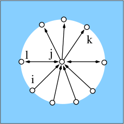
Figure 3: The neighborhood of a vertex $j$. The whole square region represents the digraph $G$, and the shaded region represents the cavity digraph $G_{\backslash j}$ after vertex $j$ and all its attached arcs are removed from $G$. The neighboring vertices of $j$ can be divided into three disjoint sets, the parent set $p(j)$, the child set $c(j)$, and the brother set $b(j)$. For instance, vertex $i\in p(j)$, $k\in c(j)$, and $l\in b(j)$. Each double-arrowed link in this figure denotes two oppositely directed arcs.

The free entropy contribution of vertex $j$ is defined as

$$\phi_{j}(x)\equiv\frac{1}{x}\ln\Bigl{[}\frac{Z(x)}{Z(x;G_{\backslash j})}\Bigr{]}\;,$$ (9)

where $Z(x;G_{\backslash j})$ denotes the partition function of the cavity digraph $G_{\backslash j}$. Under the Bethe-Peierls approximation, the explicit expression of $\phi_{j}(x)$ is

$$\phi_{j}(x)=\frac{1}{x}\ln\biggl{(}1+e^{xw_{j}}\sum\limits_{h=1}^{D}\prod\limits_{l\in b(j)}q_{l\rightarrow j}^{0}\prod\limits_{i\in p(j)}\Bigl{[}\sum\limits_{h^{\prime}=0}^{h-1}q_{i\rightarrow j}^{h^{\prime}}\Bigr{]}\prod\limits_{k\in c(j)}\Bigl{[}q_{k\rightarrow j}^{0}+\sum\limits_{h^{\prime\prime}\geq h+1}^{D}q_{k\rightarrow j}^{h^{\prime\prime}}\Bigr{]}\biggr{)}\;.$$ (10)

Consider a link $(i\rightarrow j)$ which indicates a single arc $[i,j]$ between vertices $i$ and $j$. The free entropy contribution of this link is defined as

$$\phi_{(i\rightarrow j)}(x)\equiv\frac{1}{x}\ln\Bigl{[}\frac{Z(x)}{Z\bigl{(}x;G_{\backslash[i,j]}\bigr{)}}\Bigr{]}\;,$$ (11)

where $Z\bigl{(}x;G_{\backslash[i,j]}\bigr{)}$ is the partition function of the cavity graph $G_{\backslash[i,j]}$ obtained by removing the single arc $[i,j]$ from $G$. Its explicit expression under the Bethe-Peierls approximation is

$$\phi_{(i\rightarrow j)}(x)=\frac{1}{x}\ln\biggl{(}q_{j\rightarrow i}^{0}+\sum\limits_{h_{j}=1}^{D}q_{j\rightarrow i}^{h_{j}}\Bigl{[}\sum\limits_{h_{i}=0}^{h_{j}-1}q_{i\rightarrow j}^{h_{i}}\Bigr{]}\biggr{)}\;.$$ (12)

Similarly, the free entropy contribution $\phi_{(i\Leftrightarrow j)}(x)$ of a link $(i\Leftarrow j)$ (due to the existence of arcs $[i,j]$ and $[j,i]$ of opposite direction between vertices $i$ and $j$) is expressed as

$$\phi_{(i\Leftrightarrow j)}(x)=\frac{1}{x}\ln\Bigl{(}q_{i\rightarrow j}^{0}+q_{j\rightarrow i}^{0}-q_{i\rightarrow j}^{0}q_{j\rightarrow i}^{0}\Bigr{)}\;.$$ (13)

Under the Bethe-Peierls approximation, the whole free entropy $\Phi(x)$ of digraph $G$ can be evaluated through the following simple expression:

$$\Phi(x)=\sum\limits_{j=1}^{N}\phi_{j}(x)-\sum\limits_{(i\rightarrow j)\in G}\phi_{(i\rightarrow j)}(x)-\sum\limits_{(i\Leftrightarrow j)\in G}\phi_{(i\Leftrightarrow j)}(x)\;.$$ (14)

The first term of the above expression is the sum of free entropy contributions of all the vertices. Since each link $(i\rightarrow j)$ contributes to the free entropies of vertices $i$ and $j$, the free entropy contribution of this link should be subtracted once from the total free entropy. This explains the second term of (14). Similarly the free entropy contribution of each link $(k\Leftrightarrow l)$ should be subtracted once from the total free entropy, leading to the third term of (14).

The free entropy density is computed from (14) as $\phi(x)=\frac{1}{N}\Phi(x)$. The entropy density $s$ of the system is then calculated through

$$s=-x^{2}\frac{\partial\phi(x)}{\partial x}=x\bigl{[}\phi(x)-\omega(x)\bigr{]}\;,$$ (15)

where $\omega(x)$ is the relative total weight of the occupied vertices:

$$\omega(x)\equiv\frac{1}{N}\sum\limits_{j=1}^{N}(1-q_{j}^{0})w_{j}\;.$$ (16)

To actually compute the free entropy density $\phi(x)$ and other thermodynamic quantities, we need to compute the two cavity probability distributions $p_{j\rightarrow k}^{h_{j}}$ and $p_{k\rightarrow j}^{h_{k}}$ associated with every link $(j\rightarrow k)$ and also the two distributions $p_{k\rightarrow j}^{h_{k}}$ and $p_{j\rightarrow k}^{h_{j}}$ associated with every link $(j\Leftrightarrow k)$. Under the same Bethe-Peierls approximation we can write down the following self-consistent equations for two connected vertices $j$ and $j^{\prime}$:

$$q_{j\rightarrow j^{\prime}}^{0}=\frac{1}{z_{j\rightarrow j^{\prime}}}\;,\quad\quad\quad q_{j\rightarrow j^{\prime}}^{h_{j}}=\frac{a_{j\rightarrow j^{\prime}}(h_{j})}{z_{j\rightarrow j^{\prime}}}\;,\quad\quad(1\leq h_{j}\leq D)$$ (17)

where $z_{j\rightarrow j^{\prime}}$ and $a_{j\rightarrow j^{\prime}}(h)$ are computed through the following two expressions, respectively:

$$z_{j\rightarrow j^{\prime}}=1+e^{xw_{j}}\sum\limits_{h=1}^{D}\prod\limits_{l\in b(j)\backslash j^{\prime}}q_{l\rightarrow j}^{0}\prod\limits_{i\in p(j)\backslash j^{\prime}}\Bigl{[}\sum\limits_{h^{\prime}=0}^{h-1}q_{i\rightarrow j}^{h^{\prime}}\Bigr{]}\prod\limits_{k\in c(j)\backslash j^{\prime}}\Bigl{[}q_{k\rightarrow j}^{0}+\sum\limits_{h^{\prime\prime}\geq h+1}^{D}q_{k\rightarrow j}^{h^{\prime\prime}}\Bigr{]}\;,$$ (18)

$$a_{j\rightarrow j^{\prime}}(h)=e^{xw_{j}}\prod\limits_{l\in b(j)\backslash j^{\prime}}q_{l\rightarrow j}^{0}\prod\limits_{i\in p(j)\backslash j^{\prime}}\Bigl{[}\sum\limits_{h^{\prime}=0}^{h-1}q_{i\rightarrow j}^{h^{\prime}}\Bigr{]}\prod\limits_{k\in c(j)\backslash j^{\prime}}\Bigl{[}q_{k\rightarrow j}^{0}+\sum\limits_{h^{\prime\prime}\geq h+1}^{D}q_{k\rightarrow j}^{h^{\prime\prime}}\Bigr{]}\;.$$ (19)

Notice that Eq. (17) holds for all vertices $j^{\prime}\in\partial j$, and it differs from Eq. (6) only by discarding vertex $j^{\prime}$ from the set $\partial j$. Equation (17) is referred to as the belief propagation (BP) equation. This equation together with the free entropy expression (14) forms the RS mean field theory of model (3).

The BP equation can be solved by iterations. In each time step of this iteration we consider all the vertices consecutively and in a random order, and for each vertex $j$ under consideration we update all its output cavity probabilities $q_{j\rightarrow j^{\prime}}^{h_{i}}$ using (17). The difference between the updated cavity probability $q_{j\rightarrow j^{\prime}}^{h_{i}}(t+1)$ at time $t+1$ and the old cavity probability $q_{j\rightarrow j^{\prime}}^{h_{i}}(t)$ is measured by

$$\Delta_{j\rightarrow j^{\prime}}(t)\equiv\sum\limits_{h=0}^{D}\Bigl{|}q_{j\rightarrow j^{\prime}}^{h}(t+1)-q_{j\rightarrow j^{\prime}}^{h}(t)\Bigr{|}\;.$$ (20)

If the maximal value of all the differences $\Delta_{j\rightarrow j^{\prime}}(t)$ is less than certain small threshold $\Delta$ then we regard the BP iteration as converging to a fixed point. In this work we set the convergence criterion as $\Delta=0.01$. Compared with the BP iteration process of the undirected FVS problem [24], the BP iteration for the directed FVS problem is more time- and computer memory-consuming, since each height state can have $(D+1)$ possible values.

After the BP equation converges on all the arcs we can then compute the free entropy density $\phi$ and the entropy density $s$. In addition, the mean fraction $\rho$ of vertices in the FVS is equal to the mean fraction of unoccupied vertices:

$$\rho=\frac{1}{N}\sum\limits_{j=1}^{N}q_{j}^{0}\;.$$ (21)

4.2 Application to a single directed cycle

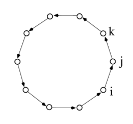
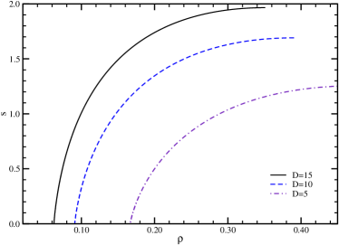
Figure 4: Replica-symmetric mean field results for a single directed cycle. (a) A directed cycle with $N=10$ vertices. (b) The entropy density $s$ versus FVS relative size $\rho$ obtained at three maximum height values $D=5$, $D=10$, and $D=15$.

As a simple illustration of the RS mean field theory, let us apply it to a digraph composed of a single directed cycle of $N$ vertices and $M=N$ arcs (in the example of Fig. 4, $N=10$). The BP equation (17) always converges for this system, and at the BP fixed point all the parent-to-child cavity distributions $q_{i\rightarrow j}^{h}$ for arcs $[i,j]$ are identical to the same probability function $q_{pc}^{h}$ which satisfies

$$q_{pc}^{0}=\frac{1}{1+e^{x}\sum\limits_{h=1}^{D}\sum\limits_{h^{\prime}=0}^{h-1}q_{pc}^{h^{\prime}}}\;,\quad\quad\quad q_{pc}^{h}=\frac{e^{x}\sum\limits_{h^{\prime}=0}^{h-1}q_{pc}^{h^{\prime}}}{1+e^{x}\sum\limits_{h=1}^{D}\sum\limits_{h^{\prime}=0}^{h-1}q_{pc}^{h^{\prime}}}\quad(h=1,2,\ldots,D)\;.$$ (22)

The unique solution of this equation is

$$q_{pc}^{0}=\frac{1}{A}\;,\quad\quad\quad q_{pc}^{h}=\frac{e^{x}}{A(A+e^{x})}\bigl{(}1+\frac{e^{x}}{A}\bigr{)}^{h}\quad(h=1,2,\ldots,D)\;,$$ (23)

where the constant $A$ is determined by $A=\bigl{(}1+\frac{e^{x}}{A}\bigr{)}^{D}$. Similarly all the child-to-parent cavity distributions $q_{j\rightarrow i}^{h}$ on the arcs $[i,j]$ are identical to the same probability function $q_{cp}^{h}$ with $q_{cp}^{0}=\frac{1}{A}$ and $q_{cp}^{h}=\frac{e^{x}}{A(A+e^{x})}\bigl{(}1+\frac{e^{x}}{A}\bigr{)}^{D+1-h}$ ($1\leq h\leq D$).

The mean field theory then predicts that the FVS relative size $\rho$, the free entropy density $\phi$, and the entropy density $s$ are

$$\rho=\frac{1}{1+\frac{e^{x}D}{A+e^{x}}}\;,\quad\quad\phi=\frac{1}{x}\ln A\;,\quad\quad s=\ln A-x(1-\rho)\;,$$ (24)

which are all independent of the cycle length $N$. As $x\rightarrow\infty$ we have $s\rightarrow 0$ and $\rho\rightarrow\frac{1}{D+1}$, see Fig. 4. The minimum FVS size $\rho_{0}$ predicted by the RS theory is $\rho_{0}=\frac{N}{D+1}$, which is higher than the true minimum size $1$ if $D<(N-1)$ and is lower than the true value if $D$ is longer than the cycle length $N$.

This exactly solvable example clearly demonstrates that the RS mean field theory is only an approximate theory. A major shortcoming of the RS theory is that it neglects all the cycle-caused long range correlations and all the cycle corrections to the free entropy $\Phi(x)$ [34, 35, 36, 37], even though the constraints in the directed FVS and FAS problems are induced by directed cycles.

In B we consider another simple random graph example to discuss more about the relationship between predicted minimum FVS relative size ($\rho_{0}$) and the parameter $D$. The numerical results shown in Fig. 9 demonstrates that the predicted value of $\rho_{0}$ decreases considerably with $D$ for an infinitely large random digraph.

4.3 Application to single random digraphs

We now perform BP iterations on two types of random digraphs, namely Erdös-Rényi (ER) digraphs and regular random (RR) digraphs [1, 2]. We generate a random digraph $G$ of $N$ vertices and $M=\alpha N$ arcs in two steps. First we generate an undirected random simple graph $G^{\prime}$ of $N$ vertices and $M$ undirected edges. Then we turn each undirected edge of $G^{\prime}$ into a directed edge (an arc) by assigning it a direction uniformly at random from the two possible directions. The resulting digraph is then the digraph $G$. An undirected ER graph $G^{\prime}$ is generated from an empty graph of $N$ vertices. Two different vertices $i$ and $j$ are randomly drawn from the whole set of $N$ vertices, if these two vertices are not yet connected we draw an edge between them. This edge addition process continues until $M$ edges have been created. An undirected RR graph has the property that each vertex is attached by exactly $d=2\alpha$ edges, therefore to generate such a graph we first assign $d$ $`$half-edges’ to each vertex, and then repeatedly glue two randomly chosen half-edges into a full edge if this full edge is neither a self-connection nor a multi-edge between two vertices.

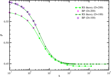
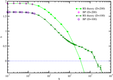
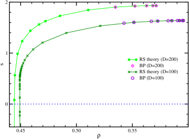
Figure 5: Replica-symmetric mean field results on ER random graphs of arc density $\alpha=10$ and uniform vertex weight $w=1$, obtained with maximal height $D=100$ and $D=200$. (a) Mean fraction $\rho$ of unoccupied vertices. (b) Entropy density $s$. (c) Entropy density $s$ as a function of FVS relative size $\rho$. The dotted lines of (b) and (c) indicate $s=0$. The BP results are obtained on a single digraph with $N=10^{5}$ vertices. The RS results are obtained by population dynamics simulations, which correspond to $N=\infty$.

The circular and diamond points of Figure 5 are the BP iteration results on a single random ER digraph with $N=10^{5}$ vertices and arc density $\alpha=10$. As the re-weighting parameter $x$ increases from zero, the relative size $\rho$ of FVS and the entropy density $s$ decrease continuously. However we find that the BP iteration process no longer converges if $x$ exceeds $2$. The non-convergence of BP iteration indicates the Bethe-Peierls approximation is no longer a good approximation at $x>2$ for this system (see also Sec. 4.2). On the other hand, when BP converges on a single digraph instance, the computed entropy density $s$ and FVS relative size $\rho$ are in good agreement with ensemble-averaged results (see next subsection).

4.4 Ensemble-averaged results

The RS mean field theory can also be used to calculate ensemble-averaged properties of random digraphs at the thermodynamic limit of $N\rightarrow\infty$. From Eq. (14) we know that to compute the free entropy density $\phi(x)$ we need only to compute the mean value of vertex contribution $\phi_{j}(x)$ over all vertices $i$ and the mean value of link contribution $\phi_{(i\rightarrow j)}(x)$ over all links $(i\rightarrow j)$ (the sum of link contributions $\phi_{(i\Leftrightarrow j)}(x)$ can be neglected since there is only a vanishing fraction of links $(i\Leftrightarrow j)$ in random ER or RR digraphs). These mean values and the FVS relative size $\rho$ are easy to compute by population dynamics simulations [31].

Corresponding to Eq. (21) for the FVS relative size $\rho$ of a single digraph, the ensemble-averaged value of $\rho$ is obtained by the following probabilistic equation (assuming all the vertex weights $w=1$)

$$\rho=\sum\limits_{d_{p}}\sum\limits_{d_{c}}P(d_{p},d_{c})\prod\limits_{i}^{d_{p}}\int\mathcal{D}q_{i\rightarrow j}Q^{(p)}[q_{i\rightarrow j}]\prod\limits_{k}^{d_{c}}\int\mathcal{D}q_{k\rightarrow j}Q^{(c)}[q_{k\rightarrow j}]$$

$$\quad\quad\quad\quad\times\frac{1}{1+e^{x}\sum\limits_{h=1}^{D}\prod\limits_{i\in p(j)}\Bigl{[}\sum\limits_{h^{\prime}=0}^{h-1}q_{i\rightarrow j}^{h^{\prime}}\Bigr{]}\prod\limits_{k\in c(j)}\Bigl{[}q_{k\rightarrow j}^{0}+\sum\limits_{h^{\prime\prime}\geq h+1}^{D}q_{k\rightarrow j}^{h^{\prime\prime}}\Bigr{]}}\;.$$ (25)

In this equation, $P(d_{p},d_{c})$ is the probability that a randomly chosen vertex has $d_{p}$ parent vertices and $d_{c}$ child vertices. For ER digraphs $P(d_{p},d_{c})$ is the product of two Poisson distributions with mean value $\alpha$, $P(d_{p},d_{c})=\frac{e^{-\alpha}d_{p}^{\alpha}}{d_{p}!}\frac{e^{-\alpha}d_{c}^{\alpha}}{d_{c}!}$, while for RR digraphs $P(d_{p},d_{c})$ is the binomial distribution $P(d_{p},d_{c})=\frac{(2\alpha)!}{2^{2\alpha}d_{p}!d_{c}!}\delta_{d_{p}+d_{c}}^{2\alpha}$. The probability functional $Q^{(p)}[q_{i\rightarrow j}]$ of Eq. (25) is the probability that the parent-to-child message on an arc $[i,j]$ is the height distribution function $q_{i\rightarrow j}^{h_{i}}$; similarly, $Q^{(c)}[q_{k\rightarrow j}]$ is the probability that the child-to-parent message on an arc $[j,k]$ is the height distribution function $q_{k\rightarrow j}^{h_{k}}$.

The ensemble-averaged expressions for the vertex free-entropy contribution $\phi_{i}$ [Eq. (10)] is very similar to Eq. (25), while the ensemble-averaged expression for the arc free-entropy contribution $\phi_{(i\rightarrow j)}$ is computed through

$$\frac{1}{x}\int\mathcal{D}q_{i\rightarrow j}Q^{(p)}[q_{i\rightarrow j}]\int\mathcal{D}q_{j\rightarrow i}Q^{(c)}[q_{j\rightarrow i}]\ln\biggl{(}q_{j\rightarrow i}^{0}+\sum\limits_{h_{j}=1}^{D}q_{j\rightarrow i}^{h_{j}}\Bigl{[}\sum\limits_{h_{i}=0}^{h_{j}-1}q_{i\rightarrow j}^{h_{i}}\Bigr{]}\biggr{)}\;.$$ (26)

In the population dynamics simulations the probability functional $Q^{(p)}[q]$ is represented by a large array of $\mathcal{M}$ cavity probability distributions $q_{j\rightarrow j^{\prime}}^{h_{j}}$ of the parent-to-child type (arcs $[j,j^{\prime}]$). Similarly $Q^{(c)}[q]$ is also represented by a large array of $\mathcal{M}$ cavity probability distributions $q_{j\rightarrow j^{\prime}}^{h_{j}}$ of the child-to-parent type (arcs $[j^{\prime},j]$). To update an element of the array $Q^{(p)}[q_{j\rightarrow j^{\prime}}]$, we first generate an in-degree $d_{j}^{(p)}$ and an out-degree $d_{j}^{(c)}$ for the parent vertex $j$ according to the cavity degree distribution

$$P^{(p)}(d_{j}^{(p)},d_{j}^{(c)})\equiv\frac{d_{j}^{(c)}P(d_{j}^{(p)},d_{j}^{(c)})}{\alpha}\;,$$ (27)

and we then select $d_{j}^{(p)}$ parent-to-child probability distributions $q_{i\rightarrow j}^{h_{i}}$ from the array $Q^{(p)}[q]$ and $(d_{j}^{(c)}-1)$ child-to-parent probability distributions $q_{k\rightarrow j}^{h_{k}}$ from the array $Q^{(c)}[q]$, finally we compute a new probability distribution $q_{j\rightarrow j^{\prime}}^{h_{j}}$ according to Eq. (17) and replace an old element of the array $Q^{(p)}[q]$ with this new element. The array $Q^{(c)}[q_{j\rightarrow j^{\prime}}]$ is updated according to the same procedure, but the degree distribution of the child vertex $j$ is changed to be

$$P^{(c)}(d_{j}^{(p)},d_{j}^{(c)})\equiv\frac{d_{j}^{(p)}P(d_{j}^{(p)},d_{j}^{(c)})}{\alpha}\;.$$ (28)

As an example, Fig. 5 shows the ensemble-averaged mean field results for ER digraphs with arc density $\alpha=10$. In our calculations the weight of each vertex $i$ is set to be $w_{i}=1$ for simplicity. The FVS relative size $\rho$ and the entropy density $s$ both decrease with the re-weighting parameter $x$, while the entropy density $s$ as a function of $\rho$ appears to be concave and its value becomes negative as $\rho$ is lower than certain threshold value $\rho_{0}(D)$ which depends slightly on the parameter $D$ (the maximal height), e.g., $\rho_{0}=0.449$ at $D=100$ and $\rho_{0}=0.444$ at $D=200$.

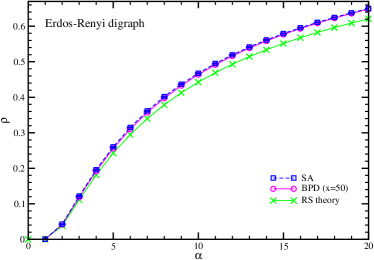
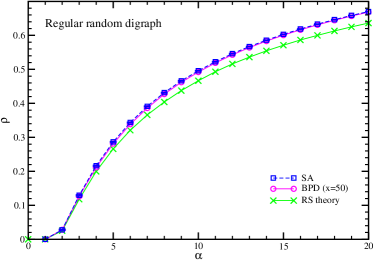
Figure 6: Comparing the theoretical prediction and algorithmic results on the FVS relative size of ER (a) and RR (b) digraphs. Cross symbols are the RS mean field predictions on the minimum FVS relative size $\rho$ obtained at $D=200$. Circular symbols (together with error bars) are the average values of the FVS relative size obtained by a single run of the BPD algorithm (with $D=200$ and $x=50$) on $96$ digraph instances of $N=10^{4}$ vertices and $M=\alpha N$ arcs. Square symbols (together with error bars) are the average values of the FVS relative size obtained by a single run of the SA algorithm (with the same parameters of [18]) on these $96$ digraph instances.

At a given value of $D$ we take the value of $\rho_{0}$ obtained by the RS population dynamics at entropy density $s=0$ as the predicted minimum relative size of FVS. The relationship between $\rho_{0}$ and the arc density $\alpha$ obtained at $D=200$ is shown in Fig. 6 for ER and RR random digraphs. In view of the discussion made in Sec. 4.2 the predicted $\rho_{0}$ should only be considered as an educated guess on the true value of FVS relative size.

5 Belief propagation-guided decimation

Through BP iteration we can obtain an estimate about the height probability distribution $q_{j}^{h_{j}}$ of each vertex $j$, see Eq. (6). This estimate might not be very accurate if the underlying Bethe-Peierls approximation is not a good approximation (especially when the BP iteration fails to converge), however it still contains very useful information for constructing a near-optimal feedback vertex set. We now describe a belief propagation-guided decimation (BPD) algorithm for solving the directed FVS problem (and also the FAS problem) on single digraph instances.

5.1 Description of the algorithm

Initially all the vertices of the digraph $G$ are declared as active, and the candidate FVS is initialized as empty, $\Gamma=\emptyset$. The BP iteration then runs on this digraph for $T_{0}$ time steps and the height probability distribution $q_{j}^{h_{j}}$ of each vertex $j$ is computed by Eq. (6). We set $T_{0}=500$ in this paper. The BPD algorithm then repeatedly performing the following fixing-and-updating procedure:

In the fixing stage, the active vertices $j$ are ranked in descending order of their empty probability $q_{j}^{0}$, and the vertices at the top $p$ percent of this ranked sequence are all added to the set $\Gamma$ and declared as inactive. We set $p=0.005$ in this paper. The digraph induced by the remaining active vertices is then simplified by repeatedly turning an active vertex into inactive if this vertex has no active parent and brother vertices, or no active child and brother vertices.

Then in the updating state, we run BP iteration on the simplified digraph of active vertices for $T$ time steps ($T=10$ in this paper). Then the height probability distributions of all the active vertices are computed by Eq. (6) again.

All the vertices in the original digraph $G$ will be turned into inactive by repeating the fixing-and-updating process. The resulting set $\Gamma$ forms a FVS of $G$. We then further polish this set by examining, in a random order, each vertex of $\Gamma$ and deleting it from $\Gamma$ if the reduced set is still a FVS. The performance of the BPD algorithm also depends on the maximal height $D$ and the re-weighting parameter $x$. For a digraph with $N$ vertices and $M$ arcs, the required memory space for running the BPD algorithm is of order $D\times M$ while the time complexity is of order $(T_{0}+T/p)\times D\times M$. The source code of the BPD algorithm is accessible at the author’s webpage (power.itp.ac.cn/$\sim$zhouhj/codes.html).

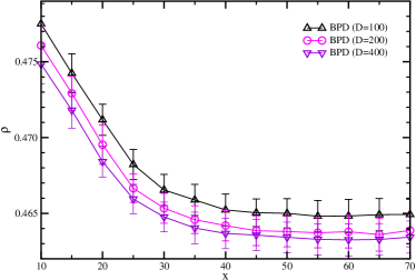
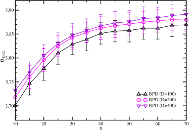
Figure 7: The performance of the BPD algorithm on $96$ random ER digraphs of $N=10^{4}$ vertices and $M=10^{5}$ arcs (arc density $\alpha=10$). (a) Mean relative size $\rho$ of the constructed FVS. (b) Mean arc density $\alpha_{DAG}$ of the resulting directed acyclic graph. The maximal height is set to $D=100$ (up triangles), $D=200$ (circles), and $D=400$ (down triangles). The other parameters of the BPD algorithm are $T_{0}=500$, $T=10$, and $p=0.005$.

Figure 7 shows the mean value of the relative sizes of constructed feedback vertex sets and the mean value of arc densities of the complementary directed acyclic digraphs, obtained by averaging the results of a single run of the BPD algorithm on $96$ random ER digraphs of arc density $\alpha=10$ and vertex number $N=10^{4}$. When the maximum height $D$ is fixed, the performance of BPD improves considerably as $x$ increases from $0$ to $30$ and then saturates as $x$ goes beyond $40$. If the re-weighting parameter $x$ is fixed but the maximal height changes from $D=100$ to $D=200$, there is considerable improvement in the performance of BPD. However if $D$ is further increased to $D=400$ the additional improvement in performance is much weaker. Based on the empirical observations of Fig. 7 we set $x=50$ and $D=200$ when applying BPD to all the other random digraph instances mentioned below, even if these digraphs have different arc density $\alpha$.

5.2 Comparison with mean field predictions

We apply the BPD algorithm to a set of ER digraphs with $N=10^{4}$ vertices and mean arc density $\alpha$ ranging from $1$ to $20$. At each value of $\alpha$ the FVS mean relative size, denoted as $\rho_{BPD}$, is computed by averaging over the results of a single run of the BPD algorithm on $96$ independent random digraph instances. When $\alpha\leq 4$ we find the value of $\rho_{BPD}$ is very close to the minimum FVS relative size $\rho_{RS}$ as predicted by the RS mean field theory at $D=200$, see Fig. 6. However, the difference between $\rho_{BPD}$ and $\rho_{RS}$ becomes noticeable at $\alpha\approx 5$ and the positive gap $(\rho_{BPD}-\rho_{RS})$ increases continuously as $\alpha$ further increases. We have tested on several digraphs of larger size $N=10^{5}$ and found that the BPD results $\rho_{BPD}$ are not sensitive to $N$. At $D=200$, the discrepancy between the RS mean field results and the BPD algorithmic results therefore is unlikely to be caused by finite-size effects. Instead we tend to believe that this gap indicates that the RS mean field prediction $\rho_{RS}$ is lower than the true minimum FVS size. We expect that the minimum FVS size obtained by the first-step replica-symmetric breaking (1RSB) mean field theory [32] will be closer to the empirical BPD results, but we have not yet carried out such an investigation. We notice that an elegant 1RSB study has been carried out in the context of the minimal contagious set problem [29], which is an inspiration for our future 1RSB work.

We also apply the BPD algorithm to a set of RR digraphs with $N=10^{4}$ vertices and arc density $\alpha$ ranging from $1$ to $20$, and compare the results with RS mean field predictions at $D=200$, see Fig. 6. When $\alpha\leq 3$ the mean FVS relative size $\rho_{BPD}$ obtained by BPD is very close to the minimum FVS relative size $\rho_{RS}$ of mean field theory, but the difference between $\rho_{BPD}$ and $\rho_{RS}$ becomes noticeable at $\alpha\approx 4$ and is more and more pronounced as $\alpha$ further increases.

5.3 Comparison with simulated annealing

Recently an efficient heuristic local algorithm was proposed in [18], which repeatedly refine the height configuration $\underline{h}$ of a digraph through simulated annealing under the constraints (1) and (2). When tested on some small digraph instances with $N\leq 1000$ vertices, the SA algorithm outperforms the greedy adaptive searching process (GRASP) [17], one of the most successful local algorithms which repeatedly reduces the number of directed cycles by deleting vertices with highest value of in- and out-degree product $d_{p}\times d_{c}$. At each elementary step of the SA algorithm a trial is proposed to update the FVS: (a) first a randomly chosen vertex $j$ of the FVS (height $h_{j}=0$) is chosen, and (b) its height $h_{j}$ is either set to a maximal value while satisfying all the out-going arcs $[j,k]$ or set to a minimal value while satisfying all the in-coming arcs $[i,j]$, and then (c) the parent vertices $i$ of all the unsatisfied arcs $[i,j]$ or the child vertices $k$ of all the unsatisfied arcs $[j,k]$ are put to the FVS ($h_{i}=0$ or $h_{k}=0$). Such a trial is accepted for sure if the resulting FVS size does not increase, otherwise it is accepted with a low probability [18].

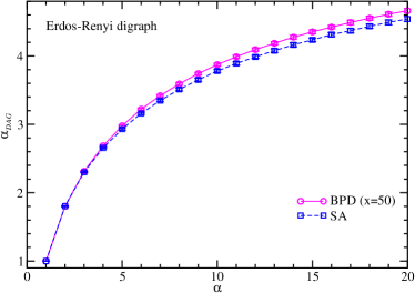
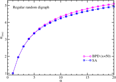
Figure 8: The arc density $\alpha_{DAG}$ of the directed acyclic graph after all the vertices of the FVS and the attached arcs are removed from the input digraph of arc density $\alpha$. Circular symbols (together with error bars) denote the results obtained by the BPD algorithm ($D=200$ and $x=50$) on $96$ digraph instances of size $N=10^{4}$, while square symbols (together with error bars) denote the results obtained by the SA algorithm (with the same parameters of [18]) on the same $96$ digraph instances. (a) ER digraph. (b) RR digraph.

Here we compare the performances of BPD and SA on large digraph instances of $N=10^{4}$ vertices, see Fig. 6 and Fig. 8. First, we notice that the mean relative sizes of FVS constructed by BPD and by SA are very close to each other both for ER and for RR digraphs. (We have also tested the BPD algorithm on the same set of small digraph instances used in [18] and found that BPD performs equally good as SA.) If we assume that the FVS solutions reached by the SA algorithm are close to optimal solutions, the results of Fig. 6 then indicate that (1) the BPD algorithm is able to construct close-to-minimum feedback vertex sets, and that (2) the RS population dynamics predictions underestimate the minimum FVS size of finite random digraph instances.

Although the sizes of FVS solutions constructed by BPD and by SA are almost equal, we find that the BPD algorithm is more likely to select a vertex of low connectivity into the FVS than the SA algorithm. As a result the DAG obtained by the BPD algorithm has considerably higher arc density (Fig. 8). In other words, if we choose the BPD algorithm instead of the SA algorithm, we can make the digraph free of directed cycles by deleting much fewer arcs. In this latter sense the BPD algorithm outperforms the SA algorithm (besides the advantage that BPD is much faster than SA). Of course both the BPD algorithm and the SA algorithm can be modified by adding another re-weighting parameter to avoid deleting highly connected vertices. Such an extension might be necessary for some practical applications.

6 Conclusion

In this paper we introduced a spin glass model (3) for the directed feedback vertex set problem, approximately solved this model by the replica-symmetric mean field theory of statistical physics, and implemented a belief propagation-guided decimation algorithm to construct nearly optimal feedback vertex sets for single digraph instances. The theory and algorithm of this paper is also applicable to the equivalent feedback arc set problem. The BPD algorithm slightly outperforms the simulated annealing algorithm (Fig. 6 and Fig. 8), it is therefore an efficient algorithm to approach a minimum feedback vertex set for single difficult digraph instances.

The RS mean field theory appears to compute a lower-bound for the FVS minimum relative size $\rho$ (Fig. 6). This theory assumes that the height states of all the neighbors of a vertex $j$ are independent of each other after vertex $j$ is deleted (Fig. 3). This approximation essentially ignores all the correlations propagated along the directed cycles (e.g., in Fig. 4 the heights $h_{i}$ and $h_{k}$ of vertices $i$ and $k$ must be strongly correlated at low temperatures even if vertex $j$ is removed). Conceptually speaking, the RS mean field theory of Sec. 4 can not be a satisfactory approach to tackle cycle constraints. Much theoretical efforts (including 1RSB mean field computations) are needed to achieve a deeper understanding on the directed FVS problem. An especially interesting but challenging question would be to design a spin glass model with truly local interactions for the cycle constraints (like the edge-constrained model for the undirected FVS problem [24]), without using height as the vertex state.

Appendix A A more restrictive spin glass model for the directed FVS problem

In this appendix we describe a more restrictive spin glass model for the directed feedback vertex set problem. The model in the main text can be regarded as a relaxed version of this model. For simplicity we assume that there is no bi-directional edges in the digraph $G$ so that the set of brother vertices of each vertex $j$ is empty: $b(j)=\emptyset$ . The partition function of this new model is defined as

$$Z(\beta)=\sum\limits_{\underline{h}}\prod\limits_{j=1}^{N}\Bigl{[}e^{-x}\delta_{h_{j}}^{0}+\delta_{h_{j}}^{1+max\{h_{i}:i\in p(j)\}}\Bigr{]}\;,$$ (29)

where $\max\{h_{i}:i\in p(j)\}$ returns the maximal height value among all the parent vertices of $j$. A height configuration $\underline{h}=(h_{1},h_{2},\ldots,h_{N})$ with $N_{0}$ zero elements will contribute a term $e^{-xN_{0}}$ to this partition function if, for every vertex $j$, the height state $h_{j}$ is either zero (vertex $j$ being unoccupied) or $h_{j}$ is exceeding the maximal height of its parent vertices by one. Such a height configuration is called a legal configuration, and all other height configurations are illegal and have no contribution to $Z(\beta)$.

There is a one-to-one correspondence between a legal configuration $\underline{h}$ of model (29) and a FVS of the digraph $G$. First, it is obvious that the set formed by all the zero-height vertices of a legal configuration $\underline{h}$ must be a FVS. Second, given any feedback vertex set $\Gamma$ of the digraph we can construct a unique legal height configuration by recursion: first assign all vertices in $\Gamma$ the height value $0$ and put them into an initially empty vertex set $S$; then assign the height value $1$ to all the vertices whose parent vertices are completely contained in set $S$ and then add these newly assigned vertices to set $S$; then repeat this process and assign the remaining vertices the height values $2$, $3$, $\ldots$, until all the vertices have been exhausted. The resulting height configuration must be a legal configuration.

The spin glass model (29) is more restrictive than the model (3). This is due to the fact that in the new model each vertex $j$ causes a many-body constraint among $j$ and all its parent vertices. For convenience of discussion let us denote by $\framebox{$\displaystyle j$}$ the constraint caused by vertex $j$. To solve this more difficult model by the replica-symmetric mean field theory, we denote by $p_{\framebox{$\displaystyle\scriptstyle{k}$}\rightarrow k}^{h_{k}}$ the probability that vertex $k$ will be in height state $h_{k}$ if it is only constrained by constraint $\framebox{$\displaystyle k$}$. Similarly, for each parent vertex $j$ of vertex $k$, we denote by $p_{\framebox{$\displaystyle\scriptstyle{k}$}\rightarrow j}^{h_{j}}$ the probability that $j$ will be in height state $h_{j}$ if it is only constrained by the constraint $\framebox{$\displaystyle k$}$. We can write down the following set of belief-propagation equations for these two height distributions:

$$p_{\framebox{$\displaystyle{\scriptstyle{k}}$}\rightarrow k}^{h_{k}}=\frac{1}{z_{{\framebox{$\displaystyle{\scriptstyle{k}}$}}\rightarrow k}}\biggl{\{}e^{-x}\delta_{h_{k}}^{0}+\delta_{h_{k}}^{1}\prod\limits_{j\in p(k)}q_{j\rightarrow\framebox{$\displaystyle\scriptstyle{k}$}}^{0}+$$

$$\hskip 56.9055pt(1-\delta_{h_{k}}^{0}-\delta_{h_{k}}^{1})\Bigl{[}\prod\limits_{j\in p(k)}Q_{j\rightarrow\framebox{$\displaystyle\scriptstyle{k}$}}^{h_{k}-1}-\prod\limits_{j\in p(k)}Q_{j\rightarrow\framebox{$\displaystyle\scriptstyle{k}$}}^{h_{k}-2}\Bigr{]}\biggr{\}}\;,$$ (30)

$$p_{\framebox{$\displaystyle\scriptstyle{k}$}\rightarrow j}^{h_{j}}=\frac{1}{z_{\framebox{$\displaystyle\scriptstyle{k}$}\rightarrow j}}\biggl{\{}e^{-x}q_{k\rightarrow\framebox{$\displaystyle\scriptstyle{k}$}}^{0}+q_{k\rightarrow\framebox{$\displaystyle\scriptstyle{k}$}}^{h_{j}+1}\prod\limits_{i\in p(k)\backslash j}Q_{i\rightarrow\framebox{$\displaystyle\scriptstyle{k}$}}^{h_{j}}+$$

$$\hskip 56.9055pt\sum\limits_{h_{k}\geq h_{j}+2}q_{k\rightarrow\framebox{$\displaystyle\scriptstyle{k}$}}^{h_{k}}\Bigl{[}\prod\limits_{i\in p(k)\backslash j}Q_{i\rightarrow\framebox{$\displaystyle\scriptstyle{k}$}}^{h_{k}-1}-\prod\limits_{i\in p(k)\backslash j}Q_{i\rightarrow\framebox{$\displaystyle\scriptstyle{k}$}}^{h_{k}-2}\Bigr{]}\biggr{\}}\;.$$ (31)

In the above equations $z_{\framebox{$\displaystyle\scriptstyle{k}$}\rightarrow k}$ and $z_{\framebox{$\displaystyle\scriptstyle{k}$}\rightarrow j}$ are two probability normalization constants; the quantity $q_{k\rightarrow\framebox{$\displaystyle\scriptstyle{k}$}}^{h_{k}}$ denotes the probability that vertex $k$ will be in height state $h_{k}$ if it is not constrained by constraint $\framebox{$\displaystyle k$}$; the quantity $Q_{j\rightarrow\framebox{$\displaystyle\scriptstyle{k}$}}^{h}$ is a partial sum defined as

$$Q_{j\rightarrow\framebox{$\displaystyle\scriptstyle{k}$}}^{h}\equiv\sum_{h_{j}=0}^{h}q_{j\rightarrow\framebox{$\displaystyle\scriptstyle{k}$}}^{h_{j}}\;,$$ (32)

where $q_{j\rightarrow\framebox{$\displaystyle\scriptstyle{k}$}}^{h_{j}}$ denotes the probability that the parent vertex $j$ of vertex $k$ will be in height state $h_{j}$ if the constraint $\framebox{$\displaystyle k$}$ is absent. The self-consistent BP equations for $q_{k\rightarrow\framebox{$\displaystyle\scriptstyle{k}$}}^{h_{k}}$ and $q_{j\rightarrow\framebox{$\displaystyle\scriptstyle{k}$}}^{h_{j}}$ are much simplier:

$$q_{k\rightarrow\framebox{$\displaystyle\scriptstyle{k}$}}^{h_{k}} = \frac{1}{z_{k\rightarrow\framebox{$\displaystyle\scriptstyle{k}$}}}\prod\limits_{l\in c(k)}p_{\framebox{$\displaystyle\scriptstyle{l}$}\rightarrow k}^{h_{k}}\;,$$ (33)

$$q_{j\rightarrow\framebox{$\displaystyle\scriptstyle{k}$}}^{h_{j}} = \frac{1}{z_{j\rightarrow\framebox{$\displaystyle\scriptstyle{k}$}}}p_{\framebox{$\displaystyle\scriptstyle{j}$}\rightarrow j}^{h_{i}}\prod\limits_{l\in c(j)\backslash k}p_{\framebox{$\displaystyle\scriptstyle{l}$}\rightarrow j}^{h_{j}}\;,$$ (34)

where again $z_{k\rightarrow\framebox{$\displaystyle\scriptstyle{k}$}}$ and $z_{j\rightarrow\framebox{$\displaystyle\scriptstyle{k}$}}$ are two probability normalization constants.

The marginal probability $q_{j}^{h_{j}}$ that vertex $j$ will be in height state $h_{j}$ in the digraph $G$ is then evaluated at a fixed-point of the BP iteration as

$$q_{j}^{h_{j}}=\frac{1}{z_{j}}p_{\framebox{$\displaystyle\scriptstyle{j}$}\rightarrow j}^{h_{j}}\prod\limits_{k\in c(j)}p_{\framebox{$\displaystyle\scriptstyle{k}$}\rightarrow j}^{h_{j}}\;,$$ (35)

with $z_{j}$ being a normalization constant. The mean fraction of unoccupied vertices (i.e., the FVS relative size) $\rho$ is computed as

$$\rho=\frac{1}{N}\sum\limits_{j=1}^{N}q_{j}^{0}\;.$$ (36)

The BP equations (30)–(34) are rather slow to iterate. Our preliminary numerical results indicated that the feedback vertex set solutions offered by this more complicated BP scheme are not better than the solutions obtained by the relaxed BP scheme of the main text. In this work we therefore give up further exploration of the model (29) of many-body interactions.

To be complete, here we also list the explicit expression for the total free entropy $\Phi(x)$ of the new model:

$$\Phi(x)=\sum\limits_{k=1}^{N}\Bigl{[}\phi_{\framebox{$\displaystyle\scriptstyle{k}$}}-d_{k}^{(c)}\phi_{k}\Bigr{]}\,$$ (37)

where $d_{k}^{(c)}\equiv|c(k)|$ is the number of child vertices of vertex $k$ (the out-degree). In this expression, $\phi_{\framebox{$\displaystyle\scriptstyle{k}$}}$ is the free entropy contribution of constraint $\framebox{$\displaystyle k$}$ and all its involved vertices, and $\phi_{k}$ is the free entropy contribution of vertex $k$. Their respective expressions are

$$\phi_{\framebox{$\displaystyle\scriptstyle{k}$}}=-\frac{1}{x}\ln\biggl{\{}e^{-x}\prod\limits_{l\in c(k)}p_{\framebox{$\displaystyle\scriptstyle{l}$}\rightarrow k}^{0}\prod\limits_{j\in p(k)}\Bigl{[}\sum\limits_{h_{j}\geq 0}p_{\framebox{$\displaystyle\scriptstyle{j}$}\rightarrow j}^{h_{j}}\prod\limits_{m\in c(j)\backslash k}p_{\framebox{$\displaystyle\scriptstyle{m}$}\rightarrow j}^{h_{j}}\Bigr{]}$$

$$\hskip 56.9055pt+\prod\limits_{l\in c(k)}p_{\framebox{$\displaystyle\scriptstyle{l}$}\rightarrow k}^{1}\prod\limits_{j\in p(k)}\Bigl{[}p_{\framebox{$\displaystyle\scriptstyle{j}$}\rightarrow j}^{0}\prod\limits_{m\in c(j)\backslash k}p_{\framebox{$\displaystyle\scriptstyle{m}$}\rightarrow j}^{0}\Bigr{]}$$

$$\hskip 56.9055pt+\sum\limits_{h_{k}\geq 2}\prod\limits_{l\in c(k)}p_{\framebox{$\displaystyle\scriptstyle{k}$}\rightarrow k}^{h_{k}}\biggl{(}\prod\limits_{j\in p(k)}\Bigl{[}\sum\limits_{h_{j}=0}^{h_{k}-1}p_{\framebox{$\displaystyle\scriptstyle{j}$}\rightarrow j}^{h_{j}}\prod\limits_{m\in c(j)\backslash k}p_{\framebox{$\displaystyle\scriptstyle{m}$}\rightarrow j}^{h_{j}}\Bigr{]}$$

$$\hskip 113.81102pt-\prod\limits_{j\in p(k)}\Bigl{[}\sum\limits_{h_{j}=0}^{h_{k}-2}p_{\framebox{$\displaystyle\scriptstyle{j}$}\rightarrow j}^{h_{j}}\prod\limits_{m\in c(j)\backslash k}p_{\framebox{$\displaystyle\scriptstyle{m}$}\rightarrow j}^{h_{j}}\Bigr{]}\biggr{)}\biggr{\}}\;,$$ (38)

$$\phi_{k}=-\frac{1}{x}\ln\biggl{\{}\sum\limits_{h_{k}}p_{\framebox{$\displaystyle\scriptstyle{k}$}\rightarrow k}^{h_{k}}\prod\limits_{l\in c(k)}p_{\framebox{$\displaystyle\scriptstyle{l}$}\rightarrow k}^{h_{k}}\biggr{\}}\;.$$ (39)

Appendix B Replica-symmetric solution for a special Random regular digraph

In Sec. 4.2 we studied a single directed cycle and found that the RS mean field predicted that the relative size $\rho_{0}$ of minimum FVS approaches zero as the maximal height parameter $D\rightarrow\infty$. In this appendix we study another exactly solvable digraph and show that for this system the value of $\rho_{0}$ may converge to a strictly positive value at $D=\infty$.

The digraph we now consider is a completely random digraph with the constraint that each vertex has exactly $\alpha$ parent vertices and $\alpha$ child vertices (i.e., the in-degree and out-degree of every vertex is an integer $\alpha$). The weight of every arc in this digraph is set to be unity. For such a random digraph the BP equation (17) has a fixed point with all the parent-to-child cavity distributions $q_{i\rightarrow j}^{h}$ for arcs $[i,j]$ being identical to the same probability function $q_{pc}^{h}$ and all the child-to-parent cavity distributions $q_{j\rightarrow i}^{h}$ being identical to the same probability function $q_{cp}^{h}$. Furthermore we find that $q_{cp}^{0}=q_{pc}^{0}$ and $q_{cp}^{h}=q_{pc}^{D+1-h}$ for $1\leq h\leq D$.

Following the general BP equation (17), we obtain the self-consistent condition for the function $q_{pc}^{h}$ as

$$q_{pc}^{0} = \frac{1}{1+e^{x}\sum\limits_{\tilde{h}=1}^{D}\Bigl{[}\sum\limits_{h^{\prime}=0}^{\tilde{h}-1}q_{pc}^{h^{\prime}}\Bigr{]}^{\alpha}\Bigl{[}\sum\limits_{h^{\prime\prime}=0}^{D-\tilde{h}}q_{pc}^{h^{\prime\prime}}\Bigr{]}^{\alpha-1}}\;,$$ (40)

$$q_{pc}^{h} = \frac{e^{x}\Bigl{[}\sum\limits_{h^{\prime}=0}^{h-1}q_{pc}^{h^{\prime}}\Bigr{]}^{\alpha}\Bigl{[}\sum\limits_{h^{\prime\prime}=0}^{D-h}q_{pc}^{h^{\prime\prime}}\Bigr{]}^{\alpha-1}}{1+e^{x}\sum\limits_{\tilde{h}=1}^{D}\Bigl{[}\sum\limits_{h^{\prime}=0}^{\tilde{h}-1}q_{pc}^{h^{\prime}}\Bigr{]}^{\alpha}\Bigl{[}\sum\limits_{h^{\prime\prime}=0}^{D-\tilde{h}}q_{pc}^{h^{\prime\prime}}\Bigr{]}^{\alpha-1}}\quad\quad\quad(h=1,2,\ldots,D)\;.$$ (41)

These two equations have only a unique solution for any fixed values of the parameters $x$ and $D$. We determine the value of $q_{pc}^{h}$ through the following numerical procedure: (1) set $q_{pc}^{0}$ to a value $q_{0}\in(0,1]$; (2) determine the value $q_{pc}^{D}$ by solving $q_{pc}^{D}=e^{x}q_{0}q_{0}^{\alpha-1}(1-q_{pc}^{D})^{\alpha}$, and then determine $q_{pc}^{1}$ according to $q_{pc}^{1}=e^{x}q_{0}q_{0}^{\alpha}(1-q_{pc}^{D})^{\alpha-1}$; (3) then determine the value of $q_{pc}^{D-1}$ by solving $q_{pc}^{D-1}=e^{x}q_{0}(q_{0}+q_{1})^{\alpha-1}(1-q_{pc}^{D}-q_{pc}^{D-1})^{\alpha}$ and then determine $q_{pc}^{2}$ according to $q_{pc}^{2}=e^{x}q_{0}(q_{0}+q_{1})^{\alpha}(1-q_{pc}^{D}-q_{pc}^{D-1})^{\alpha-1}$; (4) then continue to determine all the remaining probability items $q_{pc}^{h}$ in the same sequential maner as steps (2) and (3); (5) then compute a new value of $q_{pc}^{0}$ according to Eq. (40); (6) if $q_{pc}^{0}$ is different from the input value $q_{0}$ we then change $q_{0}$ appropriately and repeat steps (1)–(5) until convergence is reached.

At the fixed point of Eqs. (40) and (41) we then compute the relative size $\rho$ of FVS is

$$\rho=\frac{1}{1+e^{x}\sum\limits_{\tilde{h}=1}^{D}\Bigl{[}\sum\limits_{h^{\prime}=0}^{\tilde{h}-1}q_{pc}^{h^{\prime}}\Bigr{]}^{\alpha}\Bigl{[}\sum\limits_{h^{\prime\prime}=0}^{D-\tilde{h}}q_{pc}^{h^{\prime\prime}}\Bigr{]}^{\alpha-1}}\;.$$ (42)

The free entropy density $\phi$ is

$$\phi = \frac{\alpha}{x}\ln\biggl{[}1+e^{x}\sum\limits_{\tilde{h}=1}^{D}\Bigl{[}\sum\limits_{h^{\prime}=0}^{\tilde{h}-1}q_{pc}^{h^{\prime}}\Bigr{]}^{\alpha}\Bigl{[}\sum\limits_{h^{\prime\prime}=0}^{D-\tilde{h}}q_{pc}^{h^{\prime\prime}}\Bigr{]}^{\alpha-1}\biggr{]}$$ (43)

$$-\frac{(\alpha-1)}{x}\ln\biggl{[}1+e^{x}\sum\limits_{\tilde{h}=1}^{D}\Bigl{[}\sum\limits_{h^{\prime}=0}^{\tilde{h}-1}q_{pc}^{h^{\prime}}\Bigr{]}^{\alpha}\Bigl{[}\sum\limits_{h^{\prime\prime}=0}^{D-\tilde{h}}q_{pc}^{h^{\prime\prime}}\Bigr{]}^{\alpha}\biggr{]}\;.$$

The entropy density is then simply computed as $s=x\phi-x(1-\rho)$. At a given value of maximal height $D$ we can obtain the function $s(\rho)$ by performing numerical calculations at different values of $x$. The minimum relative size $\rho_{0}$ at this value of $D$ is then determined by solving $s(\rho_{0})=0$. The plus symbols of Fig. 9 are the predicted values of $\rho_{0}$ up to $D=13,107,200$ for the particular case of arc density $\alpha=20$. Qualitatively the same mean field results are obtained for other values of the arc density $\alpha$.

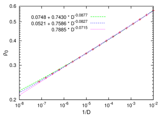
Figure 9: The predicted minimum value $\rho_{0}$ of FVS relative size for the special regular random digraph in which every vertex is connected to $20$ parent vertices and $20$ child vertices. The value of $\rho_{0}$ depends on the maximal height $D$ used in the RS mean field theory. The three fitting curves are $\rho_{0}=0.0748+0.7430D^{-0.0877}$ (long-dashed blue line), $\rho_{0}=0.0521+0.7586D^{-0.0827}$ ( dashed blue line), and $\rho_{0}=0.7885D^{-0.0715}$ (dotted red line).

Figure 9 demonstrates that $\rho_{0}$ decreases slowly with maximal height $D$. We can fit the behaviour of $\rho_{0}$ as

$$\rho_{0}=\rho_{0}^{\infty}+\frac{a}{D^{\gamma}}\;,$$ (44)

the fitting parameter $\rho_{0}^{\infty}$ is then the predicted minimum FVS relative size for an infinite random digraph. The fitted value of $\rho_{0}^{\infty}$ is sensitive to the range of $D$ values included in the fitting. For example, if we only use the data points of $10^{2}\leq D\leq 10^{5}$, we obtain $\rho_{0}^{\infty}\approx 0.075\pm 0.005$, see the green long-dashed line of Fig. 9; if we use the data points of $10^{2}\leq D<1.311\times 10^{7}$ we obtain a value $\rho_{0}^{\infty}\approx 0.052\pm 0.002$, see the blue dashed line of Fig. 9. It’s not easy for us to compute $\rho_{0}$ for $D>10^{7}$, but we anticipate that if more $\rho_{0}$ data obtained at very large $D$ values are included in the fitting, the fitted $\rho_{0}^{\infty}$ will further decrease. On the other hand, we observe that if we fix $\rho_{0}^{\infty}=0$ the fitting can not capture the asymptotic behaviour of $\rho_{0}$ at $D>10^{6}$ (see dotted red curve of Fig. 9). Therefore we believe $\rho_{0}^{\infty}$ should be strictly positive.

References

References

- [1] D.-R. He, Z.-H. Liu, and B.-H. Wang. Complex Systems and Complex Networks. Higher Education Press, Beijing, 2009.
- [2] R. Albert and A.-L. Barabási. Statistical mechanics of complex networks. Rev. Mod. Phys., 74:47–97, 2002.
- [3] L. Ermann, K. M. Frahm, and D. L. Shepelyansky. Google matrix analysis of directed networks. Rev. Mod. Phys., 87:1261–1310, 2015.
- [4] F. Li, T. Long, Y. Lu, Q. Ouyang, and C. Tang. The yeast cell-cycle network is robustly designed. Proc. Natl. Acad. Sci. USA, 101:4781–4786, 2004.
- [5] A. Veliz-Cuba, B. Aguilar, F. Hinkelmann, and R. Laubenbacher. Steady state analysis of boolean molecular network models via model reduction and computational algebra. BMC Bioinformatics, 15:221, 2014.
- [6] F. Sorrentino. Effects of the network structural properties on its controllability. Chaos, 17:033101, 2007.
- [7] Y.-Y. Liu, J.-J. Slotine, and A.-L. Barabási. Controllability of complex networks. Nature, 473:167–173, 2011.
- [8] B. Fiedler, A. Mochizuki, G. Kurosawa, and D. Saito. Dynamics and control at feedback vertex sets. I: Informative and determining nodes in regulatory networks. Journal of Dynamics and Differential Equations, 25:563–604, 2013.
- [9] A. Mochizuki, B. Fiedler, G. Kurosawa, and D. Saito. Dynamics and control at feedback vertex sets. II: A faithful monitor to determine the diversity of molecular activities in regulatory networks. J. Theor. Biol., 335:130–146, 2013.
- [10] P. Festa, P. M. Pardalos, and M. G. C. Resende. Feedback set problems. In D.-Z. Du and P. M. Pardalos, editors, Handbook of combinatorial optimization, pages 209–258. Springer, Berlin, Germany, 1999.
- [11] S. Mugisha and H.-J. Zhou. Identifying optimal targets of network attack by belief propagation. arXiv:1603.05781, 2016.
- [12] A. Braunstein, L. Dall’Asta, G. Semerjian, and L. Zdeborová. Network dismantling. arXiv:1603.08883, 2016.
- [13] M. Garey and D. S. Johnson. Computers and Intractability: A Guide to the Theory of NP-Completeness. Freeman, San Francisco, 1979.
- [14] G. Even, J. S. Naor, B. Schieber, and M. Sudan. Approximating minimum feedback sets and multicuts in directed graphs. Algorithmica, 20:151–174, 1998.
- [15] M.-C. Cai, X. Deng, and W. Zang. An approximation algorithm for feedback vertex sets in tournaments. SIAM J. Comput., 30:1993–2007, 2001.
- [16] J. Chen, Y. Liu, S. Luand B. O’sullivan, and I. Razgon. A fixed-parameter algorithm for the directed feedback vertex set problem. J. ACM, 55:21, 2008.
- [17] P. M. Pardalos, T.-B. Qian, and M. G. C. Resende. A greedy randomized adaptive search procedure for the feedback vertex set problem. J. Combinatorial Optimization, 2:399–412, 1999.
- [18] P. Galinier, E. Lemamou, and M. W. Bouzidi. Applying local search to the feedback vertex set problem. J. Heuristics, 19:797–818, 2013.
- [19] V. Bafna, P. Berman, and T. Fujito. A -approximation algorithm for the undirected feedback vertex set problem. SIAM J. Discrete Math., 12:289–297, 1999.
- [20] S. Bau, N. C. Wormald, and S. Zhou. Decycling numbers of random regular graphs. Random Struct. Alg., 21:397–413, 2002.
- [21] R. Monasson and R. Zecchina. Entropy of the k-satisfiability problem. Phys. Rev. Lett., 76:3881–3885, 1996.
- [22] M. Mézard, G. Parisi, and R. Zecchina. Analytic and algorithmic solution of random satisfiability problems. Science, 297:812–815, 2002.
- [23] M. Mézard and R. Zecchina. The random k-satisfiability problem: from an analytic solution to an efficient algorithm. Phys. Rev. E, 66:056126, 2002.
- [24] H.-J. Zhou. Spin glass approach to the feedback vertex set problem. Eur. Phys. J. B, 86:455, 2013.
- [25] J.-H. Zhao and H.-J. Zhou. Optimal discuption of directed complex networks. preprint, 2016.
- [26] C.-L. Chang and Y.-D. Lyuu. Triggering cascades on strongly connected directed graphs. In Proceedings of the Fifth International Symposium on Parallel Architectures, Algorithms and Programming (PAAP), pages 95–99. IEEE, 2012.
- [27] F. Altarelli, A. Braunstein, L. Dall’Asta, and R. Zecchina. Optimizing spread dynamics on graphs by message passing. J. Stat. Mech.: Theor. Exp., page 09011, 2013.
- [28] F. Altarelli, A. Braunstein, L. Dall’Asta, and R. Zecchina. Large deviations of cascade processes on graphs. Phys. Rev. E, 87:062115, 2013.
- [29] A. Guggiola and G. Semerjian. Minimal contagious sets in random regular graphs. J. Stat. Phys., 158:300–358, 2015.
- [30] G. Del Ferraro and E. Aurell. Dynamic message-passing approach for kinetic spin models with reversible dynamics. Phys. Rev. E, 92:010102(R), 2015.
- [31] M. Mézard and A. Montanari. Information, Physics, and Computation. Oxford Univ. Press, New York, 2009.
- [32] M. Mézard and G. Parisi. The bethe lattice spin glass revisited. Eur. Phys. J. B, 20:217–233, 2001.
- [33] H. A. Bethe. Statistical theory of superlattices. Proc. R. Soc. London A, 150:552–575, 1935.
- [34] M. Chertkov and V. Y. Chernyak. Loop series for discrete statistical models on graphs. J. Stat. Mech.: Theor. Exp., page P06009, 2006.
- [35] H. J. Zhou and C. Wang. Region graph partition function expansion and approximate free energy landscapes: Theory and some numerical results. J. Stat. Phys., 148:513–547, 2012.
- [36] J.-Q. Xiao and H. J. Zhou. Partition function loop series for a general graphical model: free-energy corrections and message-passing equations. J. Phys. A: Math. Theor., 44:425001, 2011.
- [37] H. J. Zhou, C. Wang, J.-Q. Xiao, and Z. Bi. Partition function expansion on region-graphs and message-passing equations. J. Stat. Mech.: Theo. Exp., page L12001, 2011.