Leaving Some Stones Unturned:
Dynamic Feature Prioritization
for Activity Detection in Streaming Video

Abstract

Current approaches for activity recognition often ignore constraints on computational resources: 1) they rely on extensive feature computation to obtain rich descriptors on all frames, and 2) they assume batch-mode access to the entire test video at once. We propose a new active approach to activity recognition that prioritizes “what to compute when” in order to make timely predictions. The main idea is to learn a policy that dynamically schedules the sequence of features to compute on selected frames of a given test video. In contrast to traditional static feature selection, our approach continually re-prioritizes computation based on the accumulated history of observations and accounts for the transience of those observations in ongoing video. We develop variants to handle both the batch and streaming settings. On two challenging datasets, our method provides significantly better accuracy than alternative techniques for a wide range of computational budgets.

I Introduction

Activity recognition in video is a core vision challenge. It has applications in surveillance, autonomous driving, human-robot interaction, and automatic tagging for large-scale video retrieval. In any such setting, a system that can both categorize and temporally localize activities would be of great value.

Activity recognition has attracted a steady stream of interesting research [1]. Recent methods are largely learning-based, and tackle realistic everyday activities (e.g., making tea, riding a bike). Due to the complexity of the problem, as well as the density of raw data comprising even short videos, useful video representations are often computationally intensive—whether dense trajectories, interest points, object detectors, or convolutional neural network (CNN) features run on each frame [2, 3, 4, 5, 6, 7, 8]. In fact, the expectation is that the more features one extracts from the video, the better for accuracy. For a practitioner wanting reliable activity recognition, then, the message is to “leave no stone unturned”, ideally extracting complementary descriptors from all video frames.

However, the “no stone unturned” strategy is problematic. Not only does it assume virtually unbounded computational resources, it also assumes that an entire video is available at once for batch processing. In reality, a recognition system will have some computational budget. Further, it may need to perform in a streaming manner, with access to only a short buffer of recent frames. Together, these considerations suggest some form of feature triage is needed.

Yet prioritizing features for activity in video is challenging, for two key reasons. First, the most informative features may depend critically on what has been observed so far in the specific test video, making traditional fixed/static feature selection methods inadequate. In other words, the recognition system’s belief state must evolve over time, and its priorities of which features to extract next must evolve too. Second, when processing streaming video, the entire video is never available to the algorithm at once. This puts limits on what features can even be considered each time step, and requires accounting for the feature extractors’ framerates when allocating computation.

In light of these challenges, we propose a dynamic approach to prioritize which features to compute when for activity recognition. We formulate the problem as policy learning in a Markov decision process. In particular, we learn a non-myopic policy that maps the accumulated feature history (state) to the subsequent feature and space-time location (action) that, once extracted, is most expected to improve recognition accuracy (reward) over a sequence of such actions. We develop two variants of our approach: one for batch processing, where we are free to “jump” around the video to get the next desired feature, and one for streaming video, where we are confined to a buffer of newly received frames. By dynamically allocating feature extraction effort, our method wisely leaves some stones unturned—that is, some features unextracted—in order to meet real computational budget constraints.

To our knowledge, our work is the first to actively triage feature computation for streaming activity recognition. While recent work explores ways to intelligently order feature computation in a static image for the sake of object or scene recognition [10, 11, 12, 13, 14, 15, 16, 17] or offline batch activity detection [18], streaming video presents unique challenges, as we explain in detail below. While methods for “early” detection can fire on an action prior to its completion [19, 20, 21], they nonetheless passively extract all features in each incoming frame.

We validate our approach on two public datasets consisting of third- and first-person video from over 120 activity categories. We show its impact in both the streaming and batch settings, and we further consider scenarios where the test video is “untrimmed”. Comparisons with status quo passive feature extraction, traditional feature selection approaches, and a state-of-the-art early event detector demonstrate the clear advantages of our approach.

II Related Work

II-A Activity recognition and detection

Recognizing activities is a long-standing vision challenge [1]. Current methods explore both high-level representations based on objects, attributes, or scenes [8, 3, 22, 23, 4], as well as holistic frame-level CNN descriptors [4, 5, 6, 7]. Our approach is a general algorithm for feature prioritization, and it is flexible to the descriptor type; we demonstrate instances of both types in our results. Unlike traditional activity recognition work, we account for 1) bounded computational resources for feature extraction and 2) streaming (and possibly untrimmed) input video.

Much less work addresses activity detection, which requires both categorizing and localizing an activity in untrimmed video. Common strategies are sliding temporal window search [24, 25, 26] or analyzing tracked objects [27, 28, 29, 30]. While some tracking-based methods permit incremental computation and thus can handle streaming video (e.g., [27]), they are limited to activities well-defined by a moving foreground subject. “Action-like” space-time proposals [31, 32, 33, 34] and efficient search methods [35, 36] can avoid applying classifiers to all possible video subvolumes, but they do not prioritize feature computation. A recurrent neural network learns to predict which frame in a video to analyze next for offline action detection [18]; its policy is free to hop forward and backward in time in the video to extract subsequent features, which is not possible in the streaming case we consider. Furthermore, our method pinpoints feature extraction requests to include not just when in the video to look for a single type of feature [18], but also where in the frame to look and which particular feature to extract upon looking there. Unlike our approach, all the above prior classifier-based methods assume batch access to the entire test video. Furthermore, with the exception of [18], they also assume features can be extracted on every frame.

II-B Early event detection

The goal in “early” event detection is for the detector to fire early on in the activity instance, enabling timely reactions (e.g., for human-robot interactions [19] or nefarious activity in surveillance [20]). In [19], a structured output approach learns to recognize partial events in untrimmed video. Other methods tackle trimmed streaming video, developing novel integral-histograms that permit incremental recognition [20], or an HMM model that processes more frames until its action prediction is trusted [21]. In a sense, “early” detectors eliminate needless computation. However, the goals and methods are quite different from ours. They intend to detect an action before its completion, whereas we aim to detect an action with limited computation. As such, whereas the early methods “front-load” computation—extracting all features for each incoming frame—our method targets which features to compute when, and can even skip frames altogether. Furthermore, rather than learn a static model of what the onset of an action looks like, we learn a dynamic policy that indicates which computation to perform given past observations.

II-C Fast object detection

Various ways to accelerate object detection have been explored [37, 38, 39, 40]. Cascaded and coarse-to-fine detectors (e.g., [39, 40]) determine a fixed ordering of features to quickly reject unlikely regions. In contrast, our work deals with activity recognition in video, and the feature ordering we learn is dynamic, non-myopic, and generalizes to streaming data.

II-D Active object and scene recognition in images

Recent work considers “active” and “anytime” object recognition in images [14, 15, 12, 16, 13, 10, 11, 17, 41]. The goal is to determine which feature or classifier to apply next so as to reduce inference costs and/or supply an increasingly confident estimate as time progresses. Several methods explore dynamic feature selection algorithms for object and scene recognition [14, 16, 13, 17], using strategies based on reinforcement learning [14, 12, 13, 41], or myopic information gain [17, 16]. Though focused on scene recognition in images, [17] also includes a preliminary trial for “dynamic scenes” in short trimmed videos; however, the model does not represent temporal dynamics, the data is batch-processed, and gains over passive recognition are not shown. These existing methods categorize an image (recognition), search for an object (detection) [10, 15, 12, 11] or perform structured prediction [41].

This family of methods is most relevant to our goal. However, whereas prior work performs object/scene recognition in images, we consider activity recognition in streaming video. Feature triage on video offers unique challenges. Active recognition on images is a feature ordering task: one has the entire image in hand for processing, and the results of selected observations are static and simply accumulate. In contrast, for video, features come and go, and we must update beliefs over time and prioritize future observations accordingly. Furthermore, we must represent temporal continuity (i.e., model context over both time and space) and, when streaming, respect the hard limits of the video buffer size. In terms of a Markov decision process, this translates into a much larger state-action space.

II-E Allocating computation for video

To our knowledge, no prior work studies dynamically prioritizing features for streaming activity recognition, while there is limited work prioritizing computation for other tasks in video. In [42], information gain is used to determine which object detectors to deploy on which frames for semantic segmentation. In [43], a second-order Markov model selects frames to apply a more expensive algorithm, for face detection and background subtraction. A cost-sensitive approach to multiscale video parsing schedules inference at different levels of a hierarchy (e.g., a group activity composed of individual actions) using AND-OR graphs [44, 45]. Aside from being different tasks than ours, all the above methods consider only the offline/batch scenario.

III Approach

We first formalize the problem (Sec. III-A). Then we present our approach and explain the details of its batch and streaming variants (Sec. III-B).

III-A Problem Formulation

Let $X\in\mathcal{X}$ denote a video clip and let $y\in\mathcal{Y}$ denote an activity category label. During training we have access to a set $\{(X_{1},y_{1}),\dots,(X_{T},y_{T})\}$ of video clips, each labeled by one of $L$ activity categories, $y_{i}\in\{1,\dots,L\}$. The training clips are temporally trimmed to the action of interest. At test time, we are given a novel video that may be trimmed or untrimmed. For the trimmed case, the ultimate goal is to predict the activity category label (i.e., a multi-way recognition task). For the untrimmed case, the goal is to temporally localize when an activity appears within it (i.e., a binary detection task).

First, we train an activity recognition module using the labeled videos. Let $\Psi(X)$ denote a descriptor computed for video $X$. We train an activity classifier $f:\Psi\times\mathcal{Y}\rightarrow\mathbb{R}$ to return a posterior for the specified activity category:

$$f(\Psi(X),y)=P(y|X).$$ (1)

We use one-vs-all multi-class logistic regression classifiers for $f$ and bag-of-object or CNN descriptors for $\Psi$ (details below), though other choices are possible. When training $f$, descriptors on training videos are fully instantiated using all frames. This classifier is trained and fixed prior to policy learning.

We formulate dynamic feature prioritization as a reinforcement learning problem: the system must learn a policy to request the features in sequence that will, over the course of a recognition episode, maximize its confidence in the true activity category. At test time, given an unlabeled video, inference is a sequential process. At each step $k=1,\dots,K$ of an episode we must 1) actively prioritize the next feature computation action and 2) refine the activity category prediction. Thus, our primary goal is to learn a dynamic policy $\pi$ that maps partially observed video features to the next most valuable action. This policy should be far-sighted, such that its choices account for interactions between the current request and subsequent features to be selected. Furthermore, it should respect a computational budget, meaning it conforms to constraints on the feature request costs and/or the number of inference steps permitted. We consider both batch and streaming recognition settings.

III-B Learning the Feature Prioritization Policy

We develop a solution using a Markov decision process (MDP), which is defined by the following components [46]:

• A state $s_{k}$ that captures the current environment at the $k$-th step of the episode, defined in terms of the history of extracted features and prior actions.

• A set of discrete actions $\mathcal{A}=\{a_{m}\}^{M}_{m=1}$ the system can perform at each step in the episode, which will lead to an update of the state. An action extracts information from the video.

• An instant reward $r_{k}=R(s_{k},a^{(k)},s_{k+1})$ received by transitioning from state $s_{k}$ to state $s_{k+1}$ after taking action $a^{(k)}$, defined in terms of activity recognition. The total reward is $\sum_{k}\gamma^{k}R(s_{k},a^{(k)},s_{k+1})$, where $\gamma\in[0,1]$ is a discount factor on future rewards. Larger values lead to more far-sighted policies.

• A policy $\pi:s\rightarrow a$ determines the next action based on the current state. It selects the action that maximizes the expected reward:

  $$\pi(s_{k})=\operatorname*{arg\,max}_{a}E[R|s_{k},a,\pi],$$ (2)

  for this action and future actions continuing under the same policy.

We next detail the video representation, state-action features, and rewards for the general case. Then, we define aspects specific to the batch and streaming settings, respectively.

Video Descriptors and Actions

Our algorithm accommodates a range of descriptor/classifier choices. The requirements are that the descriptor 1) have temporal locality, and 2) permit incremental updates as new descriptor instances are observed. These specs are met by popular “bag-of-X” and CNN frame features, as we will demonstrate in results, as well as others like quantized dense trajectories or human body poses.

We focus our implementation primarily on a bag-of-objects descriptor. Suppose we have object detectors for $N$ object categories. The fully observed descriptor $\Psi(X)$ is an $N$-dimensional vector, where $\Psi_{n}(X)$ is the likelihood that the $n$-th object appears (at least once) in the video clip $X$. We chose a bag-of-objects for its strength in compactly summarizing high-level content relevant to activities [4, 3, 47]. For example, an activity like “making sandwich” is definable by bread, knife, frig, etc. Furthermore, it exposes semantic temporal context valuable for sequential feature selection. For example, after seeing a mug, the system may learn to look next for either a tea bag or a coffee maker.

Each step in an episode performs some action $a^{(k)}\in\mathcal{A}$ at a designated time $t^{k}$ in the video. We define each action as a tuple $a_{m}=\langle o_{m},l_{m}\rangle$ consisting of an object and video location. Specifically, $o_{m}\in\{1,\ldots,N\}$ specifies an object detector, and $l_{m}$ specifies the space-time subvolume where to run it. The observation result $x_{m}$ of taking action $a_{m}$ is the maximum detection probability of object $o_{m}$ in volume $l_{m}$. It is used to incrementally refine the video representation $\Psi(X)$. Let $o^{(k)}=n$ denote the object specified by selected action $a^{(k)}$. Upon receiving $x^{(k)}$, the $n$-th entry in $\Psi(X^{k})\in\mathbb{R}^{N}$ is updated by taking the maximum observed probability for that object so far:

$$\Psi_{n}(X^{k})=\max\left(\Psi_{n}(X^{k}),x^{(k)}\right),$$ (3)

where $\Psi(X^{k})$ denotes the video representation based on the observation results up to the $k$-th step of the episode. The initialization of $\Psi(X)$ is explained below.

To alternatively apply our method with CNN features—which show promise for video (e.g., [6, 7, 5])—we define the representation and actions as follows. The video representation averages per-frame CNN descriptors:

$$\Psi_{n}(X^{k})=\text{mean}\left(X^{k}\right),$$ (4)

and the action becomes $a_{m}=l_{m}$, since we need to specify the temporal location alone. Though very fast CNN extraction is possible (76 fps on a CPU [51]), conventional approaches still require time linear in the length of the video, since they touch each frame. We offer sub-linear time extraction; for example, our results maintain accuracy for streaming recognition with CNNs while pulling the features from fewer than 1% of the frames.

State-Action Features

With Q-learning [46], the value of actions $E[R|s,a,\pi]$ in Eq. (2) is evaluated with $Q^{\pi}(s,a)$. It must return a value for any possible state-action pair. Our state space is very large—equal to the number of possible features times the number of possible space-time locations times their possible output values. This makes exact computation of $Q^{\pi}(s,a)$ infeasible. Thus, as common in such complex scenarios, we adopt a linear function approximation $Q^{\pi}(s,a)=\theta^{T}\phi(s,a)$, where $\phi(s,a)$ is a feature representation of a state-action pair and $\theta$ is learned from activity-labeled training clips (explained below).

The state-action feature $\phi(s,a)$ encodes information relevant to policy learning: the previous object detection results and the action history. Past object detections help the policy learn to exploit object co-occurrences (e.g., that running a laptop detector after finding soap is likely wasteful) and select discriminative but yet-unseen objects (e.g., having seen a chair, looking next for a bed or dish could disambiguate the bedroom or kitchen context, whereas a cell phone would not). The action history can also benefit the policy, letting it learn to avoid redundant selections.

Motivated by these requirements, we define the state-action feature $\phi(s,a)\in\mathbb{R}^{N+M}$ as

$$\phi(s_{k},a)=[\Psi(X^{k}),\delta t^{k}],$$ (5)

where $\Psi(X^{k})$ encodes the detection results and $\delta t^{k}$ encodes the action history. $\Psi(X^{k})\in\mathbb{R}^{N}$ is the representation defined above. The action history feature $\delta t^{k}\in\mathbb{R}^{M}$ encodes how long it has been since each action was performed in the episode, which for action $m$ is

$$\delta t^{k}(m)=t^{k}-\max_{i}\{t^{i}|a^{(i)}=a_{m}\},$$ (6)

with $\delta t^{k}(m)=0$ if $a_{m}$ has never been performed before.

To encode actions into the state-action representation $\phi(s,a)$, we learn one linear model $\theta_{a_{m}}$ for each action (details below), such that $Q^{\pi}(s,a_{m})=\theta^{T}_{a_{m}}\phi(s,a)$. In the following, we denote $\theta{=}\{\theta_{a_{m}}\}^{M}_{m=1}$.

Reward

We define a smooth reward function that rewards increasing confidence in the correct activity label, our ultimate prediction task. Intuitively, the model should continuously gather evidence for the activity during the episode, and its confidence in the correct label should increase over time and surpass all other activities by the time the computation budget is exhausted. Accordingly, for a training episode run on video $X$ with label $y^{\ast}$, we define the reward:

$$R(s_{k},a^{(k)},s_{k+1})=f(\Psi(X^{k+1}),y^{\ast})-f(\Psi(X^{k}),y^{\ast}).$$ (7)

With this definition, a new action gets no “credit” for confidence attributable to previous actions. We found that rewarding accuracy increases per unit time performs similarly to training multiple policies targeting fixed budgets. Moreover, the proposed reward has the advantage that we can run the policy for as long as desired at test time, which is essential for streaming video. Fixed-budget policies, though common in RL, are ill-suited for streaming data since we cannot know in advance the test video’s duration and the budget to allocate.

Dynamic Feature Prioritization Policy

We learn the policy $\pi$ using policy iteration [46]. Policy iteration is an iterative algorithm that alternates between generating training samples given a policy $\pi^{(i)}$ parametrized by $\theta^{(i)}$ and learning $\theta^{(i+1)}$ given the generated training samples. We describe the steps within one iteration next.

Given the policy $\pi^{(i)}$ learned from the previous iteration, new training samples are generated by running recognition episode on all videos following $\pi^{(i)}$. For each video, the recognition episode will result in a series of three tuple $\{(a^{(k)},\phi(s_{k},a^{(k)}),r_{k})\}_{k=1}^{K_{j}}$, where the length $K_{j}$ is the number of actions performed when recognizing video $v_{j}$. Each three tuple corresponds to one action in the episode, and we collect the corresponding action, state-action-feature and reward during recognition. The target value for $Q^{\pi}(s,a)$ can be computed as

$$E[R|s_{k},a,\pi]=\sum_{k}^{K_{j}}\gamma^{k}r_{k},$$ (8)

following the definition of total reward after finishing the recognition episode. Therefore, we can transform the three tuples into $(a_{k},\phi(s_{k},a^{(k)}),E[R|s_{k},a^{(k)},\pi])$, and learning $\theta^{(i+1)}$ from the three tuples becomes a regression problem

$$E[R|s_{k},a^{(k)},\pi]=\theta^{T}_{a^{(k)}}\phi(s_{k},a^{(k)}),$$ (9)

where we solve it using ridge regression. The algorithm then iterates, generating new samples using $\theta^{(i+1)}$. We run a fixed number of iterations to learn the policy

To improve exploration, we apply $\epsilon$-greedy strategy in the recognition episode during data generation. The $\epsilon$-greedy strategy picks the action that has the maximum $Q^{\pi}(s,a)$ with probability $1-\epsilon$ and a random action with probability $\epsilon$. We use random policy for $\pi^{(0)}$ in the first iteration to generate samples, and we use all the samples generated during iteration $1\sim i$ to learn $\theta^{(i+1)}$.

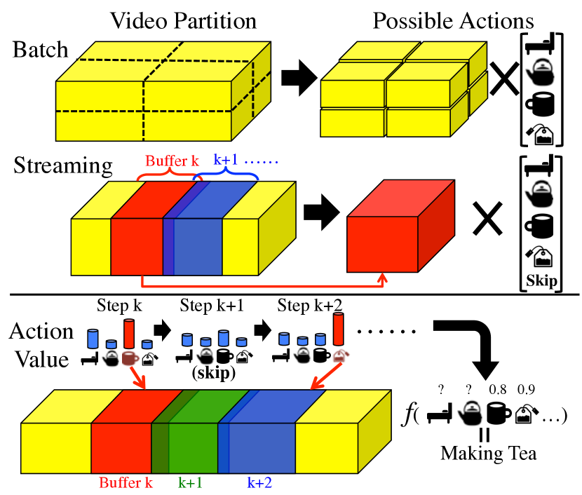
Figure 1: Action spaces. Top: In batch, the whole video is divided into subvolumes, and actions are defined by the volume and object category to detect. Middle: In streaming, the video is divided into segments by the buffer at each step, and actions are the object category to detect in the buffer plus a “skip” action. Bottom: Our method learns a video-specific policy to dynamically select a sequence of useful features to extract.

III-B1 Batch Recognition Setting

In the batch recognition setting, we have access to the entire test video throughout an episode, and the budget is the total resources available for feature computation, i.e., as capped by episode length $K$. In this case, our model is free to run an object detector at arbitrary locations. Most existing activity recognition work assumes this setting, though without imposing a computation limit. It captures the situation where one has an archive of videos to be recognized offline, subject to real-world resource constraints (e.g., auto-tagging YouTube clips under a budget of CPU time).

Each candidate location $l_{m}$ in the action set is a spatio-temporal volume. Its position and size is specified relative to the length of the entire clip, so that the number of possible actions is constant even though video lengths may vary. We use non-overlapping volumes splitting the video in half in each dimension. See Figure 1, top. Note that while the bag-of-objects discards order, the action set preserves it. That means our policy can learn to exploit the space-time layout of objects if/when beneficial to feature prioritization (e.g., learning it is useful to look for a washing machine after a laundry basket, or an pot above a stove).

In the batch setting, performing the same action at different steps in the episode will produce the same observation. Without loss of generality, we define the time an action is performed as a constant $t^{k}{=}const.\,\forall k$, and the action history feature $\delta t^{k}$ becomes a binary indicator showing whether an action has been performed in the episode. We forbid the policy to choose actions that have been performed since they provide no new information.

By design, the bag-of-objects is accumulated over time. We impute the observations of un-performed actions by exploiting previously learned object co-occurrence statistics. Let $\tilde{x}\in\mathbb{R}^{M}$ represent the observation results of all actions on a video, where the $m$-th dimension $\tilde{x}_{m}=x_{m}$ corresponds to the result of $m$-th action. The vector $\tilde{x}$ represents the object configuration in a video, and we learn its probability $p(\tilde{x})$ on the same data that trains the activity recognizer $f$ using a Gaussian Mixture Model (GMM):

$$p(\tilde{x})=\sum_{i=1}^{n}w_{i}\mathcal{N}(\tilde{x}|\mu_{i},\Sigma_{i}),$$ (10)

where we enforce a diagonal $\Sigma_{i}$ for computational efficiency. At test time, the model can be partitioned as

$$\tilde{x}=\begin{bmatrix}\tilde{x}_{u}\\ \tilde{x}_{p}\end{bmatrix},\;\mu_{i}=\begin{bmatrix}\mu_{iu}\\ \mu_{ip}\end{bmatrix},\;\Sigma_{i}=\begin{pmatrix}\Sigma_{iu}&0\\ 0&\Sigma_{ip}\end{pmatrix},$$ (11)

where $\tilde{x}_{p}$ corresponds to the observation results of performed actions and $\tilde{x}_{u}$ to un-performed actions. We estimate $\tilde{x}_{u}$ using its expected value over the conditional probability $p(\tilde{x}_{u}|\tilde{x}_{p})$, i.e.

$$\langle\tilde{x}_{u}\rangle=\sum^{n}_{i=1}w^{\prime}_{i}\mu_{ip},$$ (12)

where

$$w^{\prime}_{i}=\frac{w_{i}\mathcal{N}(\tilde{x}_{p}|\mu_{ip},\Sigma_{ip})}{\sum_{i}w_{i}\mathcal{N}(\tilde{x}_{p}|\mu_{ip},\Sigma_{ip})}.$$ (13)

III-B2 Streaming Recognition Setting

In the streaming setting, recognition takes place at the same time the video stream is received, so the model can only access frames received before the current time step. Further, the model has a fixed size buffer that operates in a first-in-first-out manner; its feature requests may only refer to frames in the current buffer. Though largely unexplored for activity recognition, the streaming scenario is critical for applications with stringent resource constraints. For example, when capturing long-term surveillance video or wearable camera data, it may be necessary to make decisions online without storing all the data.

The feature extractor can process a fixed number of frames per second, and this rate indirectly determines the resource budget. That is, the faster the feature extractors can run, the more of them we can apply as the buffer moves forward. A recognition episode ends when it reaches the end of a video stream.

The action space consists of the $N$ object detectors (or alternatively, the single CNN descriptor); an action’s space-time location $l_{m}$ is always the entire current buffer. We further define a skip action $a_{0}$, which instructs the model to wait until the next frame arrives without performing any feature extraction. Thus, for streaming, the number of actions equals the number of objects plus one ($M{=}N{+}1$). See Figure 1, middle. The skip action saves computation when the model expects a new observation will not benefit the recognition task. For example, if the model is confident that the video is taken in a bedroom, and all un-observed objects would appear only in the bathroom, then forcing the system to detect new objects is wasteful.

Because new frames may arrive and old frames may be discarded during an action, the video content available to the model will change between steps; performing the same action at different steps yields different observations. To connect the video content in the buffer and the actions in the episode, we define the time $t^{k}$ of the $k$-th action using the last frame number in the buffer when the action was issued by the policy.

While we assume so far the video contains only the target activity, i.e. the video is trimmed to the span of the activity, our method generalizes to untrimmed activity detection in the streaming environment. In that case, the target activity only occurs in part of the video, and the system must identify the span where the activity happens. This is non-trivial in the streaming environment.

To handle the streaming input, we pose the problem in terms of frame-level labeling: we predict a label for each frame as it is received, and the activity detector must optimize accuracy across all frames. However, we do not estimate the activity label from a single frame alone. Rather, we predict each frame’s label using the temporal window around it. For every newly arrived frame, we consider all the windows shorter than an upper bound $\beta$ that end at the frame. We predict the label of each window based on the same representation as trimmed video, and we select the one with highest confidence as the prediction result of the target frame. Note that this requires storing only the descriptors for recent history of length $\beta$, but keeping no video beyond the current buffer. The activity recognizer $f$ is a binary classifier trained to determine whether the target activity occurs in the window, and actions are terminated when a new frame arrives.

IV Experiment

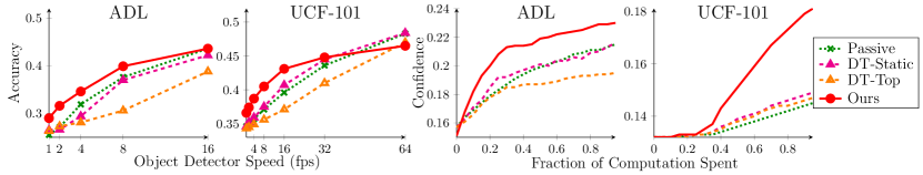
Figure 2: Streaming recognition result. Left: Recognition accuracy as a function of object detector speed. Right: Confidence score improvement as the episode progresses.

IV-A Experiment Setting

Datasets

We evaluate on two datasets: the Activities of Daily Living [3] (ADL) and UCF-101 [52]. ADL consists of 313 egocentric videos recorded by 14 subjects, labeled with $L{=}18$ activity categories (e.g., making coffee, using computer). Following [3], we train $f$ in a leave-one-subject-out manner. Our policy is learned on a disjoint set of 110 clips (those used in [3] for training object detectors). As observations $x^{(k)}$, we use the provided object detector outputs for $N{=}26$ categories (1 fps). UCF-101 consists of 13,320 YouTube videos covering $L{=}101$ activities. We use the provided training splits to train $f$, reserve half of the test splits for policy learning, and average results over all 6 splits. As observations $x^{(k)}$, we use the object detector outputs for $N{=}75$ objects, kindly shared by the authors of [4], which are frame-level scores (no bbox). For CNN frame descriptors, we use the fc-7 activation of VGG-16 [53] from Caffe Model Zoo (1 fps). The video clips average 78 and 19 seconds for ADL and UCF, respectively.

To create test data and policy learning data for the untrimmed experiments, we concatenate multiple clips following [19, 35]. Although concatenation may introduce discontinuity in content, it resembles scenarios in real videos. For example, it is similar to the video where the recorder walks from one room to another and starts the next activity. We concatenate five trimmed video clips for one un-trimmed video. For each positive clip, we generate five un-trimmed videos by placing the positive clip in different temporal location and drawing four negative clips for other locations randomly. We sort the categories by their trimmed full observation results, and take the top 8 for untrimmed experiments. In all, we obtain 8,410 (UCF) and 3,130 (ADL) untrimmed sequences, with lengths averaging 2-7 minutes, respectively. For all experiments with trimmed data, (streaming/batch) we use the datasets as-is and test all 18 (ADL) and 101 (UCF) activity categories.

Baselines

We compare to several methods:

• Passive: selects the next action randomly. It represents the most direct mapping of existing activity recognition methods to the resource-constrained regime. The system does not actively decide which features to extract.

• Object-Preference [4]: a static feature selection heuristic employed for bag-of-objects activity recognition. It prioritizes objects that appear frequently in each activity. We average $x_{m}$ per activity and order $a_{m}$ based on its maximum response over all activities. Though the authors intend this metric to identify the most discriminative objects—not to sequence feature extraction—it is a useful reference point for how far one can get with static feature selection.

• Decision tree (DT): a static feature ordering method. We learn a DT to recognize activities, where the attribute space consists of the Cartesian product of object detectors and subvolume locations ($l_{m}$). We sort the selected attributes by their Gini importance [54]. In the streaming case, we test two variations: DT-Static, where we cycle through the features in that order, and DT-Top, where we take only the top $P$ features and repeatedly apply all those object detectors on each frame. $P$ is equal to the object detector framerate. Thus, DT-Top runs as many detectors as it can at framerate, prioritizing those expected to be most discriminative.

• Max-Margin Early Event Detector (MMED) [19]: a state-of-the-art early event detector designed for untrimmed streaming video. It aims to fire on the activity as soon as possible after its onset. We implement it based on structure SVM solver BCFW [55] and apply the authors’ default parameter settings. The same window search process as in the untrimmed variant of our method is used for prediction, with a window size ranging from 1 to $\beta$ frames.

Implementation Details

We run 8 iterations of policy iteration, with $\gamma{=}0.4$. We initialize $\epsilon{=}0.5$ for $\epsilon$-greedy exploration, and decrease by $0.1$ each iteration with lower bound $0.05$. For the streaming case, we use the video framerate inherited from ADL (1 fps), and evaluate over a range of object detector framerates. We fix the buffer size to half the median clip length, 25 seconds. We set the window size upper bound $\beta$ to one-third of the number of object categories to avoid the model observing all objects within the window. For all methods, we initialize $\Psi(X)$ with features computed in the first frame in the streaming case.

IV-B Streaming Activity Recognition

First we test the streaming setting. In this case, feature extraction speed (e.g., object detector speed) dictates the action budget: the faster the features can be extracted, the more can be used while keeping up with the incoming video framerate. We stress that to our knowledge, no prior activity recognition work considers feature triage for streaming video.

Figure 2 (left 2 plots) shows the final recognition accuracy at the episode’s completion, as a function of the object detectors’ speed. Our method performs better than the rest, across the range of detector speeds. Overall, our method reduces cost by 80% and 50% on UCF and ADL, respectively. The left side of the plots is most interesting; by definition all methods will converge in accuracy once the object detector framerate equals the number of possible objects to detect (26 for ADL and 75 for UCF). DT-Top is the weakest method for this task. It repeatedly uses only the most informative features, but they are insufficient to discriminate the 18 to 101 different activities. This result shows the necessity of instance-dependent feature selection, which our method provides.

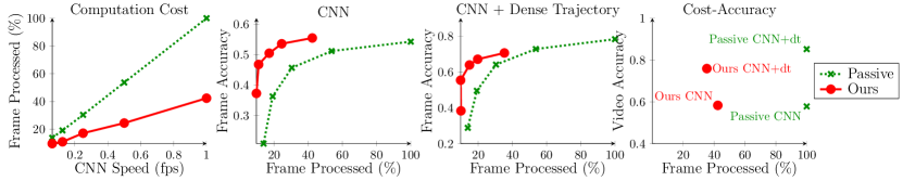
Figure 3: Streaming recognition result on UCF-101 using CNN frame features.

Figure 2 (right 2 plots) shows the confidence score (of the ground truth activity) improvement over the course of the episodes. Here we apply the 8 fps detector. The baseline methods improve their prediction smoothly, which indicates that they collect meaningful detection results at the same rate throughout the episode. In contrast, our method begins to improve rapidly after some point in the episode. This shows that it starts to collect more useful information once it has explored the novel video sufficiently. Because UCF uses about 4$\times$ more objects in the representation, it takes more computation (actions) before the representation converges.

$a^{(k)}$	Result	Observed Obj.	Possible Activities	$a^{(k+1)}$
TV	+	None	Watch-TV	TV-remote
	-	Kettle	Watch-TV/Make-tea	Tea-bag
	-	Bottle	Drink-water	Fridge
Tap	+	Dent-floss	Brush-teeth	Soap-passive
	-	Dish	Wash-dish/Watch-TV	Tap
	-	Soap-passive	Wash-hand	Soap-active

TABLE I: Excerpts of policies learned from ADL in the streaming case. “+” and “-” indicate whether the object is detected at step-$k$. Observed objects are those observed before $a^{(k)}$, and possible activities are the most likely activities predicted at step-$k$.

Table I shows example excerpts of learned policies with objects. Here we see, for example, how our approach learns to detect objects that can verify current activity hypothesis or differentiate ambiguous activities, e.g., tap does not co-occur with TV, so seeing tap rules out “Watch-TV.” It also demonstrates detailed memory such that it looks for objects that have been observed before but in a different status (actively being used by the recorder vs. passively sitting there).

Next, we show the visual examples of the learned policy in action. Figure 4 shows the policy recognizing a video clip from ADL with bag-of-object observation. In the first example, the policy observes a mug-cup and identify the activity as either reading book or watching TV. It then looks for tv-remote to disambiguate the two activities. In the second example, the policy looks for tea-bag to recognize whether the activity is making tea or draying hand. After observing tea-bag, it looks for mug-cup to verify its prediction.

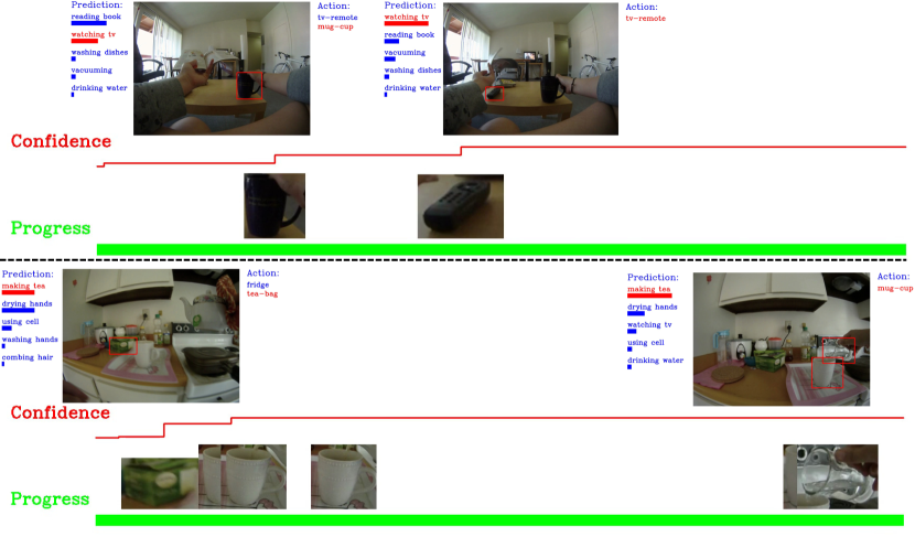
Figure 4: Two example recognition episodes on ADL with bag-of-object observation under streaming recognition setting.

Figure 5 shows the policy recognizing video clips from UCF-101 with per-frame CNN observation. The policy usually processes several frames at the beginning and decides the following frames are unlikely to be informative to the activity. Therefore, it starts skipping frames and resumes processing at a more distant frames which may provide more distinct evidence such as a closer view of the activity or different pose of the subject. From the first three examples, we can see the number of frames skipped and the number of frames processed is dependent on the observed content. For example, in the third episode, the abrupt scene change decreases the confidence significantly, and the policy spends more computation to verify its prediction. Finally, the last episode shows a failure case where the policy fails to stop computation even if the prediction is fairly stable.

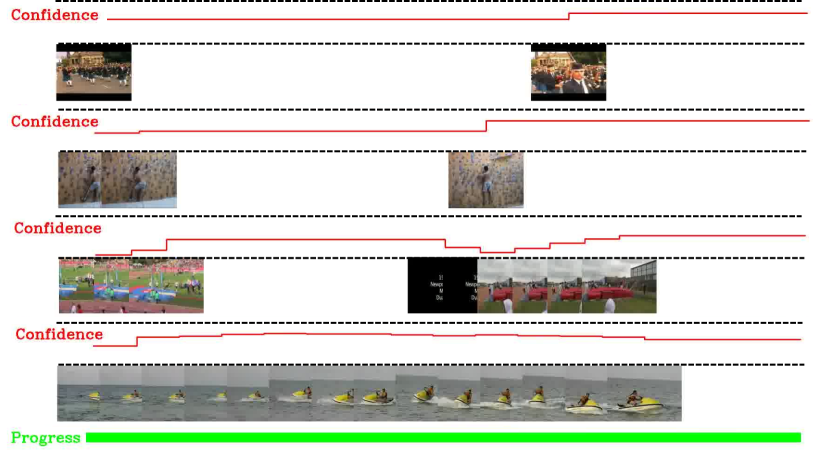
Figure 5: Four example recognition episodes on UCF-101 with CNN observation under streaming recognition setting.

Figure 3 shows our method has clear advantages if applied with CNN features as well. Here the DT baselines are not applicable, since there is only one feature type; the question is whether to extract it or not. The Passive baseline uniformly distributes its frame selections. The left plot shows that no matter the framerate of the CNN extractor, our method requires less than half of the frames to achieve the same accuracy. The second plot shows our method achieves peak accuracy looking at just a fraction of the streaming frames, where the accuracy is measured over every step in the recognition. Our algorithm skips 80% of the frames, but still achieves over 90% of the ultimate accuracy obtained using all frames. With the base sampling rate of 1 fps, processing 20% of the frames means we extract features for only 0.8% of the entire video.

In the third plot, we further combine dense trajectories (dt) with the CNN features to show that our method can benefit from more powerful features without modification. The right plot compares the cost-accuracy tradeoff between the ultimate multi-class accuracy achieved by our streaming method vs. that attained using exhaustive feature extraction. We obtain similar accuracies with substantially less computation.

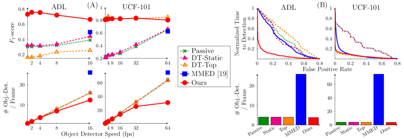
Figure 6: Streaming untrimmed detection results, with comparison to [19]. (A): Accuracy (top, higher is better) and computation cost (bottom) as a function of object detector framerate. (B): Activity monitoring operating curves (top, lower is better) and corresponding computational costs (bottom) per method.

IV-C Untrimmed Video Activity Detection

Next we evaluate streaming detection for untrimmed video. This setting permits comparison with the state of the art MMED [19] “early” activity detector.

Since we must predict whether each frame is encompassed by the target activity, we measure accuracy with the $F_{1}$-score. While we assume the episode terminates after reaching the end of the video stream in our algorithm, in some applications it may be sufficient to identify the occurrence of the activity and then terminate the episode. Therefore, we further compare the detection timeliness using the Activity Monitoring Operating Curve (AMOC), following [19]. AMOC is the normalized time to detection (NT2D) vs. the false positive rate curve. The lower the value, the better the timeliness of the detector.

In Figure 6(A), the top plots show the $F_{1}$-scores. Overall, our method performs the best in terms of accuracy. On ADL, we achieve nearly twice the accuracy of all baselines until the object detector speed reaches 16 fps. On UCF, our method is comparable to the best baseline, DT-Top. Whereas DT-Top is weak on UCF for the multi-class recognition scenario (see above), it fares well for binary detection on this dataset. This is likely because the UCF activities are often discriminated by one or few key objects, and we give the baselines the advantage of pruning the object set to those most responsive on each activity.

The bottom two plots in Figure 6(A) show the actual number of object detectors run. Our method reduces computation cost significantly under high object detector speeds, thanks to its ability to forgo computation with the “skip” action. In particular, it performs 50% fewer detections under 64 fps on UCF while maintaining accuracy. On the other hand, the baseline methods’ cost grows linearly with the object detector speed.

Figure 6(B) shows the AMOC under 4 fps detection speed (top, see appendix for others) and the associated computational costs (bottom). Despite the fact our reward function does not specifically target this metric, our method achieves excellent timeliness in detection. MMED performs second best on the metric, but it incurs much higher computation cost than ours, as shown by the bar charts. This is because MMED is trained to fire early, but always extracts all features in the frames it does process.

IV-D Batch Activity Recognition

Finally, we test the batch setting. We evaluate accuracy as a function of the computation budget—the fraction of all possible actions the algorithm performs (i.e., the number of features it extracts, normalized by video length). “All possible” features would be extracting all features in all frames (1 fps).

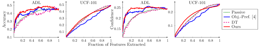
Figure 7: Batch recognition accuracy/confidence score vs. computational budget.

Figure 7 shows the results. Our method outperforms the baselines, especially when the computation budget is low ($<0.5$). In fact, extracting only 30% of the features on ADL, we achieve the same accuracy as with all features. Without a budget constraint, the video representation will converge to that of the full observation—no matter what method is used; that is, all methods must attain the same accuracy on the rightmost point on each plot. Our method shows more significant gains on ADL than UCF. We think this reflects the fact that the object categories for ADL are tailored well for the activities (e.g., household items), whereas the object bank for UCF is more diverse. Furthermore, ADL has more objects in any single activity, offering more signal for our method to learn. Object-Pref [4] is next best on ADL, though it is noticeably weaker on UCF because it does not account for the temporal redundancy of the dataset, i.e., a responsive object will be equally responsive over the entire video. Our method is 2.5 times faster than this nearest competing baseline.

Surprisingly, the Decision Tree (DT) baseline performs similarly to Passive. (Note that DT-Static only is used; DT-Top is applicable only for the streaming case.) We attempted to improve its accuracy by learning it on the same features as $f$, i.e., dropping the subvolumes from the attributes and running one object detector over the entire video for each action. However, this turned out to be worse due to redundant/wasteful detections. This shows the importance of coping with partially observed results, which the proposed method can do.

Our contribution is not a new model for activity recognition, but instead a method that enables activity recognition for existing features/classifiers without exhaustive feature computation. This means the accuracies achieved with “all features” is the key yardstick to hold our results against. Nonetheless, to put in context with other systems: the base batch recognition model we employ gets results slightly better than the state-of-the-art on ADL [3, 56] and within 4.5-11% of the state-of-the-art using comparable features on UCF [4, 5](see Figure 3, right two plots). We suspect the UCF gap is due to our use of max-pooling (vs. average) and logistic regression.

V Conclusions

We developed a dynamic feature extraction strategy for activity recognition under computational constraints. On two diverse datasets, our method shows competitive recognition performance under various resource limitations. It can be used to consistently achieve better accuracy under the same resource constraint, or meet a given accuracy using less resources. In future work we plan to investigate policies that reason about variable cost descriptors.

Appendix A Streaming Recognition

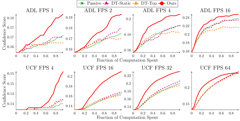
Figure 8: Streaming recognition accuracy under different object detector speed. These plots go with the one in Figure 2 above.

We show the confidence score improvement during recognition episodes with an 8 fps object detector speed in Section IV-B. For other object detector speeds, please refer to Figure 8. The results are consistent with that of 8 fps, where our method performs better than others under all object detector speeds, and the performance of different methods become more similar as the detector speed becomes faster. We do not show the results of 1 and 2 fps on UCF, because UCF videos are on average shorter, and for detectors that slow the recognition episodes consist of single action for videos shorter than the buffer size, making the curves meaningless.

Note the number of object $N{=}26$ for ADL and $N{=}75$ for UCF, and using object detector speed that exceed the number of object will reduce the problem to full observation of the video. Therefore, we show 32 fps and 64 fps results only for UCF.

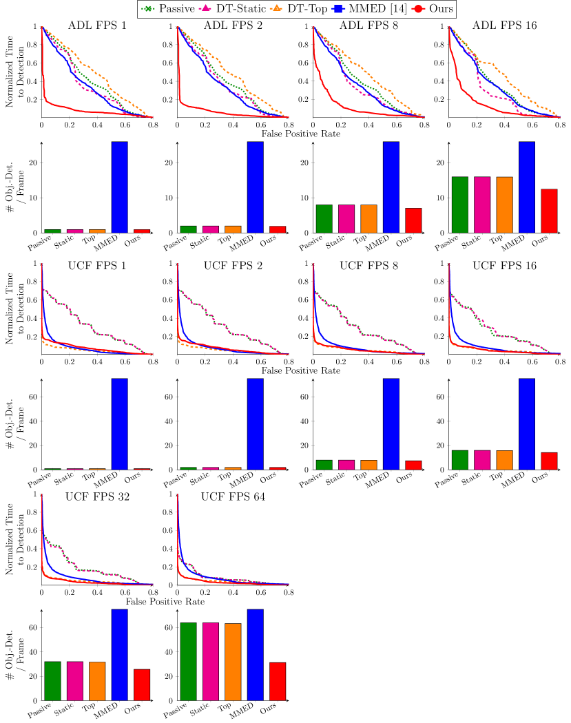
Figure 9: AMOC under different object detector speed. These plots go with the ones in Figure 6 above.

Appendix B Un-trimmed Video Activity Detection

In Figure 6, we show AMOC under 4 fps object detector speed. For the complete result, please refer to Figure 9 which shows AMOC under all other object detector speeds. Similar to the result in the paper, our method achieves excellent timeliness under all object detector speeds. Also, we can see more clearly how our method reduces computational cost under a high object detector speed. It uses only half of the computation on UCF under 64 fps object detector speed while remaining the best performing method.

References

- [1] J. K. Aggarwal and M. S. Ryoo, “Human activity analysis: A review,” ACM Computing Surveys, vol. 43, no. 3, April 2011.
- [2] H. Wang and C. Schmid, “Action recognition with improved trajectories,” in ICCV, 2013.
- [3] H. Pirsiavash and D. Ramanan, “Detecting activities of daily living in first-person camera views,” in CVPR, 2012.
- [4] M. Jain, J. C. van Gemert, and C. G. M. Snoek, “What do 15,000 object categories tell us about classifying and localizing actions?” in CVPR, 2015.
- [5] K. Simonyan and A. Zisserman, “Two-stream convolutional networks for action recognition in videos,” in NIPS, 2014.
- [6] Z. Xu, Y. Yang, and A. Hauptman, “A discriminative cnn video representation for event detection,” in CVPR, 2015.
- [7] S. Zha, F. Luisier, W. Andrews, N. Srivastava, and R. Salakhutdinov, “Exploiting image-trained cnn architectures for unconstrained video classification,” in BMVC, 2015.
- [8] D. Han, L. Bo, and C. Sminchisescu, “Selection and context for action recognition,” in ICCV, 2009.
- [9] Y.-C. Su and K. Grauman, “Leaving some stones unturned: Dynamic feature prioritization for activity detection in streaming vide,” Department of Computer Science The University of Texas at Austin, Tech. Rep. AI15-05, December 2015.
- [10] N. Butko and J. Movellan, “Optimal scanning for faster object detection,” in CVPR, 2009.
- [11] S. Vijayanarasimhan and A. Kapoor, “Visual recognition and detection under bounded computational resources,” in CVPR, 2010.
- [12] S. Karayev, T. Baumgartner, M. Fritz, and T. Darrell, “Timely object recognition,” in NIPS, 2012.
- [13] G. Dulac-Arnold, L. Denoyer, N. Thome, and M. Cord, “Sequentially generated instance-dependent image representations for classification,” in ICLR, 2014.
- [14] S. Karayev, M. Fritz, and T. Darrell, “Anytime recognition of objects and scenes,” in CVPR, 2014.
- [15] A. Gonzalez-Garcia, A. Vezhnevets, and V. Ferrari, “An active search strategy for efficient object class detection,” in CVPR, 2015.
- [16] T. Gao and D. Koller, “Active classification based on value of classifier,” in NIPS, 2011.
- [17] X. Yu, C. Fermuller, C. L. Teo, Y. Yang, and Y. Aloimonos, “Active scene recognition with vision and language,” in CVPR, 2011.
- [18] S. Yeung, O. Russakovsky, G. Mori, and L. Fei-Fei, “End-to-end learning of action detection from frame glimpses in videos,” in CVPR, 2016.
- [19] M. Hoai and F. D. la Torre, “Max-margin early event detectors,” in CVPR, 2012.
- [20] M. Ryoo, “Human activity prediction: Early recognition of ongoing activities from streaming videos,” in ICCV, 2011.
- [21] J. Davis and A. Tyagi, “Minimal-latency human action recognition using reliable-inference,” Image and Vision Computing, vol. 24, pp. 455––472, 2006.
- [22] B. Yao, X. Jiang, A. Khosla, A. Lin, L. Guibas, and L. Fei-Fei, “Human action recognition by learning bases of action attributes and parts,” in ICCV, 2011.
- [23] M. Rohrbach, M. Regneri, M. Andriluka, S. Amin, M. Pinkal, and B. Schiele, “Script data for attribute-based recognition of composite activities,” in ECCV, 2012.
- [24] Y. Ke, R. Sukthankar, and M. Hebert, “Efficient visual event detection using volumetric features,” in ICCV, 2005.
- [25] O. Duchenne, I. Laptev, J. Sivic, F. Bach, and J. Ponce, “Automatic annotation of human actions in video,” in ICCV, 2009.
- [26] S. Satkin and M. Hebert, “Modeling the temporal extent of actions,” in ECCV, 2010.
- [27] G. Medioni, R. Nevatia, and I. Cohen, “Event detection and analysis from video streams,” Trans. Pattern Analysis and Machine Intelligence, vol. 23, no. 8, pp. 873–889, 2001.
- [28] A. Yao, J. Gall, and L. van Gool, “A hough transform-based voting framework for action recognition,” in CVPR, 2010.
- [29] A. Kläser, M. Marszałek, C. Schmid, and A. Zisserman, “Human focused action localization in video,” in International Workshop on Sign, Gesture, Activity, 2010.
- [30] T. Lan, Y. Wang, and G. Mori, “Discriminative figure-centric models for joint action localization and recognition,” in ICCV, 2011.
- [31] G. Yu and J. Yuan, “Fast action proposals for human action detection and search,” in CVPR, 2015.
- [32] M. Jain, J. van Gemert, H. Jegou, P. Bouthemy, and C. Snoek, “Action localization with tubelets from motion,” in CVPR, 2015.
- [33] G. Gkioxari and J. Malik, “Finding action tubes,” in CVPR, 2015.
- [34] J. C. van Gemert, M. Jain, E. Gati, and C. G. M. Snoek, “Apt: Action localization proposals from dense trajectories,” in BMVC, 2015.
- [35] C.-Y. Chen and K. Grauman, “Efficient activity detection with max-subgraph search,” in CVPR, 2012.
- [36] G. Yu, J. Yuan, and Z. Liu, “Unsupervised random forest indexing for fast action search,” in CVPR, 2011.
- [37] M. A. Sadeghi and D. Forsyth, “30hz object detection with dpm v5,” in ECCV, 2014.
- [38] J. Yan, Z. Lei, L. Wen, and S. Li, “The fastest deformable part model for object detection,” in CVPR, 2014.
- [39] P. Viola and M. Jones, “Rapid object detection using a boosted cascade of simple features,” in CVPR, 2001.
- [40] M. Pedersoli, A. Vedaldi, and J. Gonzalez, “A coarse-to-fine approach for fast deformable object detection,” in CVPR, 2011.
- [41] D. J. Weiss and B. Taskar, “Learning adaptive value of information for structured prediction,” in NIPS, 2013.
- [42] V. Karasev, A. Ravichandran, and S. Soatto, “Active frame, location, and detector selection for automated and manual video annotation,” in CVPR, 2014.
- [43] D. Chen, M. Bilgic, L. Getoor, and D. Jacobs, “Dynamic processing allocation in video,” Pattern Analysis and Machine Intelligence, IEEE Transactions on, vol. 33, no. 11, pp. 2174–2187, 2011.
- [44] M. R. Amer, D. Xie, M. Zhao, S. Todorovic, and S.-C. Zhu, “Cost-sensitive top-down/bottom-up inference for multiscale activity recognition,” in ECCV, 2012.
- [45] M. Amer, S. Todorovic, A. Fern, and S.-C. Zhu, “Monte carlo tree search for scheduling activity recognition,” in ICCV, 2013.
- [46] S. Russell and P. Norvig, Artificial Intelligence: A Modern Approach. Pearson, 2010.
- [47] A. Gupta and L. S. Davis, “Objects in action: An approach for combining action understanding and object perception,” in CVPR, 2007.
- [48] R. Girshick, J. Donahue, T. Darrell, and J. Malik, “Rich feature hierarchies for accurate object detection and semantic segmentation,” in CVPR, 2014.
- [49] P. F. Felzenszwalb, R. B. Girshick, D. McAllester, and D. Ramanan, “Object detection with discriminatively trained part based models,” PAMI, vol. 32, no. 9, pp. 1627–1645, 2010.
- [50] S. Ren, K. He, R. Girshick, and J. Sun, “Faster R-CNN: Towards real-time object detection with region proposal networks,” in NIPS, 2015.
- [51] Nvidia, “Gpu-based deep learning inference: A performance and power analysis,” in Whitepaper, 2015.
- [52] K. Soomro, A. R. Zamir, and M. Shah, “Ucf101: A dataset of 101 human actions classes from videos in the wild,” arXiv preprint arXiv:1212.0402, 2012.
- [53] K. Simonyan and A. Zisserman, “Very deep convolutional networks for large-scale image recognition,” arXiv preprint arXiv:1409.1556, 2014.
- [54] L. Breiman, “Random forests,” Machine learning, vol. 45, no. 1, pp. 5–32, 2001.
- [55] S. Lacoste-Julien, M. Jaggi, M. Schmidt, and P. Pletscher, “Block-coordinate Frank-Wolfe optimization for structural svms,” in ICML, 2013.
- [56] T. McCandless and K. Grauman, “Object-centric spatio-temporal pyramids for egocentric activity recognition,” in BMVC, 2013.