Lattice Gauge Theories and Spin Models

Abstract

The Wegner $Z_{2}$ gauge theory-$Z_{2}$ Ising spin model duality in $(2+1)$ dimensions is revisited and derived through a series of canonical transformations. The Kramers-Wannier duality is similarly obtained. The Wegner $Z_{2}$ gauge-spin duality is directly generalized to SU(N) lattice gauge theory in $(2+1)$ dimensions to obtain the SU(N) spin model in terms of the SU(N) magnetic fields and their conjugate SU(N) electric scalar potentials. The exact & complete solutions of the $Z_{2},U(1),SU(N)$ Gauss law constraints in terms of the corresponding spin or dual potential operators are given. The gauge-spin duality naturally leads to a new gauge invariant magnetic disorder operator for SU(N) lattice gauge theory which produces a magnetic vortex on the plaquette. A variational ground state of the SU(2) spin model with nearest neighbor interactions is constructed to analyze SU(2) gauge theory.

I Introduction

In 1971 Franz Wegner, using duality transformations, showed that in two space dimensions $Z_{2}$ lattice gauge theory can be exactly mapped into a $Z_{2}$ Ising model describing spin half magnets wegner . This is the earliest and the simplest example of the intriguing gauge-spin duality. Wegner’s work, in turn, was strongly motivated by the self-duality of planar Ising model discovered by Kramers and Wannier 30 years earlier km . Such alternative dual descriptions have been extensively discussed in the past as they are useful to understand theories and their phases at a deeper level thmds ; hooft ; banks ; fradsuss ; kogrev ; savit ; horn ; dualsup ; baal ; sharatram ; manu . In the context of QCD, the duality transformations have been studied to understand color confinement via dual superconductivity thmds ; hooft ; dualsup ; baal and to extract topological degrees of freedom banks ; savit ; sharatram ; manu . They may relate the important and relevant degrees of freedoms at high and low energies providing a better understanding of non-perturbative issues in low energy QCD. The duality ideas in the Hamiltonian framework are also relevant for the recent quest to build quantum simulators for abelian and non-abelian lattice gauge theories using cold atoms in optical lattices reznik . In these cold atom experiments, the (dual) spin description of SU(N) lattice gauge theory should be useful as there are no exotic, quasi-local Gauss law constraints to be implemented at every lattice site coldatomgl . The duality methods and the resulting spin models, without redundant local gauge degrees of freedom, can also provide more efficient tensor network, variational ansatzes for the low energy states of SU(N) lattice gauge theories tn .

In this work, we start with a brief overview of Kramers-Wannier and Wegner dualities within the Hamiltonian framework. We show that these old, well-established spin-spin and gauge-spin dualities can be constructively obtained through a series of iterative canonical transformations. These canonical transformation techniques are easily generalized to SU(N) lattice gauge theory to obtain the equivalent dual SU(N) spin model without any local gauge degrees of freedom. Thus using canonical transformations we are able to treat spin, abelian and non-abelian dualities on the same footing. In $(2+1)$ dimensions the spin operators in the dual spin models are the scalar $Z_{2},U(1),SU(N)$ magnetic fields and their conjugate electric scalar potentials respectively. These spin operators solve the $Z_{2},U(1)$ and $SU(N)$ Gauss laws.

The Kramers-Wannier and Wegner dualities naturally lead to construction of disorder operators and order-disorder algebras kogrev ; fradsuss ; horn . In both cases the disorder operators are simply the dual spin operators creating $Z_{2}$ kinks and $Z_{2}$ magnetic vortices on plaquettes respectively. Note that these creation operators are highly non-local in terms of the operators of the original Ising model or $Z_{2}$ gauge theory. Therefore without duality transformations they are difficult to guess. We generalize these elementary duality ideas to non-abelian gauge theories after briefly recapitulating them in the simpler $Z_{2}$ contexts mentioned above. In particular, we exploit SU(N) dual spin operators to construct a new gauge invariant disorder operator for SU(N) lattice gauge theory. Further, like in $Z_{2}$ lattice gauge theory, the non-abelian order-disorder algebra involving SU(N) Wilson loops and SU(N) disorder operators is worked out. The interesting role of non-localities in non-abelian duality resulting in the solutions of SU(N) Gauss laws and production of local vortices is discussed. For the sake of clarity and continuity, the SU(N) gauge theory results will always be discussed in the background of the corresponding Ising model, $Z_{2}$ gauge theory results. The similar features amongst them are emphasized and the differences are also pointed out.

In the context of $Z_{2}$ gauge theory in $(2+1)$ dimensions, the two essential features of Wegner duality wegner are

• it eliminates all unphysical gauge degrees of freedom mapping it into $Z_{2}$ spin model with a $Z_{2}$ global symmetry. There are no $Z_{2}$ Gauss law constraints in the dual $Z_{2}$ spin model.

• it maps the interacting (non-interacting) terms in the $Z_{2}$ lattice gauge theory Hamiltonian into non-interacting (interacting) terms in the $Z_{2}$ spin model Hamiltonian resulting in the inversion of the coupling constant.

It is important to note that the above gauge-spin duality is through the loop description of $Z_{2}$ lattice gauge theory. The original Hamiltonian is written in terms of fundamental $Z_{2}$ electric fields and their conjugate magnetic vector potentials. The $Z_{2}$ magnetic fields are not fundamental and obtained from magnetic vector potentials. On the other hand, in the dual Ising model the fundamental spin degrees of freedom are the $Z_{2}$ magnetic fields and their conjugate electric scalar potentials. Now the electric fields are not fundamental and are obtained from the electric scalar potentials. We arrive at this dual spin description through a series of canonical transformations. They convert the initial electric fields, magnetic vector potentials into the following two mutually independent physical & unphysical classes of operators:

1. $Z_{2}$ spin or plaquette loop operators: representing the physical $Z_{2}$ magnetic fields and their conjugate electric scalar potentials over the plaquettes (see Figure 5-a),

2. $Z_{2}$ string operators: representing the $Z_{2}$ electric fields and the $Z_{2}$ flux operators of the unphysical string degrees of freedom. These strings isolate all $Z_{2}$ gauge degrees of freedom (see Figure 5-b).

The interactions of spins in the first set are described by Ising model. The corresponding physical Hilbert space is denoted by ${\cal H}^{p}$. The second complimentary set, containing $Z_{2}$ string operators, represents all possible redundant gauge degrees of freedom. We show that the Gauss law constraints freeze all strings leading to the Wegner gauge-spin duality within ${\cal H}^{p}$. Further, the electric scalar potentials are shown to be the solutions of the $Z_{2}$ Gauss law constraints. Note that no gauge fixing is required to obtain the dual description. We show that the above duality features also remain valid when these canonical/duality transformations are generalized to SU(N) lattice gauge theory. As in the $Z_{2}$ case, the SU(N) Kogut-Susskind link operators get transformed into the physical spin/loop and unphysical string operators. Again the SU(N) strings are frozen and the dual SU(N) spin operators provide all solutions of SU(N) Gauss law constraints. In fact, these SU(N) canonical transformations have been discussed earlier in the context of loop formulation of SU(N) lattice gauge theories msplb ; msprd . The motivation was to address the issue of redundancies of Wilson loops or equivalently solve the SU(N) Mandelstam constraints. We now exploit them in the context of non-abelian duality.

The plan of the paper is as follows. In section II, we discuss the canonical transformation techniques to systematically obtain Kramers-Wannier, Wegner and then SU(N) dualities. The compact U(1) lattice gauge theory duality can also be easily obtained from the SU(N) duality by ignoring the non-abelian, non-local terms. In section II.1, we start with the simplest Kramers-Wannier duality in the Ising model. The order-disorder operators, their algebras and creation, annihilation of kinks are briefly discussed for the sake of uniformity and later comparisons km ; kadanoff ; fradsuss ; kogrev ; savit ; horn . In section 2, we extend these canonical transformations to discuss Wegner duality in $2+1$ dimensions. We again obtain the old and well established results fradsuss ; kogrev ; savit ; wegner ; horn with canonical transformations as the new ingredients. The $Z_{2}$ gauge theory order-disorder operators, their algebras and $Z_{2}$ magnetic vortices are briefly summarized. In section II.3, the $Z_{2}$ canonical transformations are generalized to SU(N) lattice gauge theories leading to a SU(N) spin model. As mentioned before the SU(N) discussions are parallel to the $Z_{2}$ discussions for clarity. A comparative summary of $Z_{2}$ gauge-spin and SU(N) gauge-spin operators is given in Table 1. At the end of section II.3, we construct the new SU(N) disorder operator. The special case of ’t Hooft disorder operator is discussed. The Wilson-’t Hooft loop algebra is derived. The last section III is devoted to variational analyses of the truncated SU(N) spin model. A simple ‘single spin’ variational ground state of the dual SU(N) spin model is constructed. The Wilson loop in this ground state is shown to have area law behavior. In Appendix A, we discuss explicit constructions of $Z_{2}$ Wegner duality through canonical transformations. In Appendix B, we discuss the highly restrictive, non-local structure of SU(N) duality transformations. We explicitly show the non-trivial cancellations of infinite number of terms required to solve the SU(N) Gauss law constraints by the dual SU(N) spin operators. In part 2 of Appendix B, another set of non-trivial cancellations are shown to hold for the SU(N) disorder operator to have a local physical action in the original Kogut-Susskind formulation. In the case of much simpler $Z_{2}$ Wegner duality such cancellations are obvious. In Appendix C, we show that the ‘single spin’ variational state satisfies Wilson’s area law. In Appendix D, the expectation value of the truncated dual spin Hamiltonian is computed in the variational ground state. The expectation value of the non-local part of the spin Hamiltonian in the above disordered variational ground state is shown to vanish. This shows that non-local terms appearing with higher powers of coupling $(g^{n},n\geq 3)$ may be treated perturbatively as $(g^{2}\rightarrow 0)$ for the continuum.

Throughout this work, we use Hamiltonian formulation of lattice gauge theories ks with open boundary conditions. We work in two space dimensions on a finite lattice $\Lambda$ with ${\cal N}\left(=({\sf N}+1)\times({\sf N}+1)\right)$ sites,  ${\cal L}\left(=2{\sf N}({\sf N}+1)\right)$ links, ${\cal P}\left(={\sf N}^{2}\right)$ plaquettes satisfying: ${\cal L}={\cal P}+\left({\cal N}-1\right)$. A lattice site is denoted by $(\vec{n})$ or $(m,n)$ with $m,n=0,1,\cdots,{\sf N}$. The links are denoted by $(l)$ or $(m,n;~{}\hat{i})$ with $i=1,2$. The plaquettes are denoted by the co-ordinates of their upper right corner and sometimes by $p,p^{\prime}$ etc.. Any conjugate pair operator $P,X$ satisfying the corresponding conjugate canonical commutation relations will be denoted by $\{P;X\}$. In Ising model, Ising gauge theory, they are the Pauli spin operators $\{\sigma_{1};\sigma_{3}\}$, $\{\mu_{1};\mu_{3}\}$. In SU(N) lattice gauge theory, they are the Kogut-Susskind electric fields, link operators $\{E^{a};U_{\alpha\beta}\}$. Similarly, the canonically conjugate SU(N) spin, string operators in the dual spin models are defined in the text.

II Duality and Canonical Transformations

II.1 Kramers-Wannier duality

Kramers Wannier duality was the first and the simplest duality, apart from electromagnetism, to be constructed. As a prelude to the construction of dualities in $Z_{2}$ and SU(N) lattice gauge theories, we apply canonical transformations to $(1+1)$ dimensional Ising model to get the Kramers-Wannier duality. The Ising Hamiltonian in one space dimension is in terms of the canonically conjugate operators $\{\sigma_{1};\sigma_{3}\}$ at every lattice site satisfying,

$$\hskip 42.67912pt\sigma_{1}^{2}(m)=1;\hskip 42.67912pt\sigma_{3}^{2}(m)=1;~{}~{}~{}~{}~{}~{}~{}$$ (1)

$$\sigma_{1}(m)\sigma_{3}(m)=-\sigma_{3}(m)\sigma_{1}(m)~{}~{}{\textrm{o}r}~{}~{}[\sigma_{1}(m),\sigma_{3}(m)]_{+}=0.$$

The Hamiltonian is

$$H~{}=~{}\sum_{m=0}^{\infty}\Big{[}\sigma_{1}(m)-\lambda~{}\sigma_{3}(m)\sigma_{3}(m+1)\Big{]}.$$ (2)

The Kramers-Wannier duality is obtained by the following iterative canonical transformations along a line with $\bar{\sigma}_{3}(m=0)\equiv\sigma_{3}(m=0)$ and $\bar{\sigma}_{1}(m=0)\equiv\sigma_{1}(m=0)$:

$$\mu_{1}(m)\equiv\bar{\sigma}_{3}(m)\sigma_{3}(m+1),$$

$$\mu_{3}(m)=\bar{\sigma}_{1}(m)$$ (3)

$$\bar{\sigma}_{3}(m+1)=\sigma_{3}(m+1),$$

$$\bar{\sigma}_{1}(m+1)=\bar{\sigma}_{1}(m)\sigma_{1}(m+1)=\mu_{3}(m)\sigma_{1}(m+1).$$

The above canonical transformations iteratively replace the conjugate pair $\{\sigma_{1}(m);\sigma_{3}(m)\}$ or equivalently $\{\bar{\sigma}_{1}(m);\bar{\sigma}_{3}(m)\}$ by a new conjugate pair $\{\mu_{1}(m);\mu_{3}(m)\}$. These new pairs are mutually independent and also satisfy the canonical relations (1). Unlike gauge theories (to be discussed in the next section), there are no spurious (string) degrees of freedom. This process is graphically illustrated in Figure 1. The relations (3) lead to,

$$\mu_{3}(m)=\prod_{s=0}^{m}\sigma_{1}(s).$$ (4)

The relations (4) can be easily inverted to give $\sigma_{1}(m)=\mu_{3}(m)\mu_{3}(m-1)$ with the convention $\mu_{3}(m=-1)\equiv 1$. The Ising model Hamiltonian can now be rewritten in its self-dual form in terms of the new dual conjugate pairs $\{\mu_{1}(m);\mu_{3}(m)\}$:

$$H~{}=~{}\sum_{m=0}^{\infty}\Big{[}\mu_{3}(m)\mu_{3}(m+1)-\lambda~{}\mu_{1}(m)\Big{]}.$$ (5)

Therefore,

$$H(\sigma;\lambda)=\lambda^{-1}H(\mu;\lambda^{-1}).$$

This is the famous Kramers-Wannier self duality. As expected, duality has interchanged the interacting and non interacting parts of the Hamiltonian on going from the $\{\sigma_{1},\sigma_{3}\}$ to the dual $\{\mu_{1},\mu_{3}\}$ variables. In other words, duality/canonical transformations (3) map strong coupling region to the weak coupling region and vice versa.

II.1.1 Ising disorder operator

In Ising model the magnetization operator, $\sigma_{3}(m)$ is the order operator as its expectation value measures the degree of order of the $\sigma_{3}$ variables. It is zero for $\lambda<\lambda_{c}$ and non-zero for $\lambda>\lambda_{c}$. This implies that the $\lambda>\lambda_{c}$ phase spontaneously breaks the global $Z_{2}$ symmetry: $\sigma_{3}\rightarrow-\sigma_{3}$. On the other hand, the dual Hamiltonian (5) implies that it is natural to define $\mu_{3}(m)$ as a disorder operator kogrev ; fradsuss ; horn . The vacuum expectation value ${}_{\lambda}\langle 0|\mu_{3}(m)|0\rangle{}_{\lambda}$ is the disorder parameter. We also note that the disorder operator $\mu_{3}({x_{0}})$ acting on a completely ordered state (all $\sigma_{3}(m)=+1$ or $-1$), flips all $\sigma_{3}$ spins at $m<{x}_{0}$ and creates a kink at $x_{0}$. The resulting kink state is orthogonal to the original ordered state and the expectation value of the disorder operator $\mu_{3}$ in an ordered state vanishes:

$${}_{{}_{\lambda=\infty}}\langle 0|\mu_{3}(m)|0\rangle_{{}_{\lambda=\infty}}=0,\hskip 14.22636pt{}_{{}_{\lambda=\infty}}\langle 0|\sigma_{3}(m)|0\rangle_{{}_{\lambda=\infty}}=1.$$ (6)

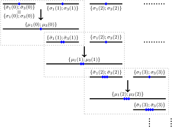
Figure 1: Kramers-Wannier duality through canonical transformations. The first three steps of duality or canonical transformations in (3) are illustrated.

Figure 2: Duality and ordered & disordered phases of $(1+1)$ dimensional Ising model kogrev ; fradsuss ; horn .

Figure 3: Duality between $Z_{2}$ lattice gauge theory and $Z_{2}$ (Ising) spin model. The initial and the final conjugate pairs $\{\sigma_{1};\sigma_{3}\}$ and $\{\mu_{1};\mu_{3}\}$, are defined on the links and the plaquettes or dual sites respectively. The corresponding SU(N) duality is illustrated in Figure 9.

On the other hand, at $\lambda=0$, the dual description (5) implies that the Ising model is in ordered state with respect to $\mu_{3}$. As a consequence, the disorder parameter does not vanish and order parameter vanishes:

$${}_{{}_{\lambda=0}}\langle 0|\mu_{3}(m)|0\rangle_{{}_{\lambda=0}}=1,\hskip 28.45274pt{}_{{}_{\lambda=0}}\langle 0|\sigma_{3}(m)|0\rangle_{{}_{\lambda=0}}=0.$$ (7)

The relations (6), (7) are illustrated in Figure 2.

II.2 Wegner duality and $Z_{2}$ Spin Model

$Z_{2}$ and $Z_{N}$ lattice gauge theories are the simplest theories with gauge structure and many rich features. Due to their enormous simplicity compared to $U(1)$ or non-abelian lattice gauge theories and the presence of a confining phase, they have been used as a simple theoretical laboratory to test various confinement ideas horn . They also provide an explicit realization of the Wilson-’t Hoofts algebra of order and disorder operators characterizing different possible phases of the SU(N) gauge theories hooft ; horn . In 1964, Schultz, Mattis and Lieb showed that the two-dimensional $Z_{2}$ Ising model is equivalent to a system of locally coupled fermions schultz . This result was later extended to $Z_{2}$ lattice gauge theory which also allows an equivalent description in terms of locally interacting fermions fradkinf . These are old and well known results. In the recent past, $Z_{2}$ $(Z_{N})$ lattice gauge theories have been useful to understand quantum spin models fradkinb , quantum computations kitaev , tensor network or matrix product states taka and their topological properties wen , cold atom simulations reznik and entanglement entropy polik . In view of these wide applications, the $Z_{2}$ $(Z_{N})$ lattice gauge theories and associated duality transformations are important in their own right.

The $Z_{2}$ lattice gauge theory involves $Z_{2}$ conjugate spin operators $\{\sigma_{1}(l);\sigma_{3}(l)\}$ on the link $l\in\Lambda$. The anti-commutation relations amongst these conjugate pairs on every link $l$ are

$$\sigma_{1}(l)~{}\sigma_{3}(l)+\sigma_{3}(l)~{}\sigma_{1}(l)=0.$$ (8)

They further satisfy: ${\sigma}_{3}(l)^{2}={\sigma}_{1}(l)^{2}=1$. In order to maintain a 1-1 correspondence with SU(N) lattice gauge theory (discussed in the next section), it is convenient to identify the conjugate pairs $\{\sigma_{1}(l);\sigma_{3}(l)\}$ with $Z_{2}$ electric field, $E(l)$ and $Z_{2}$ vector potential, $A(l)$ as:

$$\sigma_{1}(l)=e^{i\pi E(l)},~{}~{}~{}~{}~{}~{}\sigma_{3}(l)=e^{iA(l)}.$$ (9)

Above $E(l)\equiv\{0,1\}$ and $A(l)\equiv\{0,\pi\}$. A basis of the two dimensional Hilbert space on each link $l$ is chosen to be the eigenstates $\ket{\pm,l}$ of $\sigma_{3}(l)$ with eigenvalue $\pm 1$ with $\sigma_{1}(l)$ acting as a spin flip operator:

$$\sigma_{3}(l)\ket{\pm,l}=\pm\ket{\pm,l},~{}~{}~{}~{}~{}\sigma_{1}(l)|\pm,l\rangle=|\mp,l\rangle.$$ (10)

The $Z_{2}$ lattice gauge theory Hamiltonian is given by

$$H =-\sum_{l\in\Lambda}\sigma_{1}(l)-\lambda\sum\limits_{p\in\Lambda}\sigma_{3}(l_{1})\sigma_{3}(l_{2})\sigma_{3}(l_{3})\sigma_{3}(l_{4})$$

$$\equiv H_{E}+\lambda H_{B}.$$ (11)

In (11) $\sigma_{3}(l_{1})\sigma_{3}(l_{2})\sigma_{3}(l_{3})\sigma_{3}(l_{4})$ represents the product of $\sigma_{3}$ operators along the four links of a plaquette. The sum over $l$ and $p$ in (11) are the sums over all links and plaquettes respectively. The parameter $\lambda$ is the $Z_{2}$ gauge theory coupling constant. The first term $H_{E}$ and the second term $H_{B}$ in (11) represent the $Z_{2}$ electric and magnetic field operators respectively. The electric field operator $\sigma_{1}(l)$ is fundamental while the latter is a composite of the four $Z_{2}$ magnetic vector potential operators $\sigma_{3}(l)$ along a plaquette. After a series of canonical transformations, the above characterization of electric, magnetic field will be reversed. More explicitly, the dynamics will be described by the Hamiltonian (11) rewritten in terms of the fundamental magnetic field (the second term) and the electric field operator (the first term) will be composite of the dual electric scalar potentials (see (28a) and (II.2.3)). The same feature will be repeated in the SU(N) case discussed in the next section.

The Hamiltonian (11) remains invariant if all 4 spins attached to the 4 links emanating from a site $n$ are flipped simultaneously. This symmetry operation is implemented by the Gauss law operator ${\cal G}$:

$${\cal G}(n)\equiv\prod_{l_{n}}\sigma_{1}(l_{n})$$ (12)

at lattice site $n\in\Lambda$. In (12), $\prod_{l_{n}}$ represents the product over 4 links (denoted by $l_{n}$) which share the lattice site $n$ in two space dimensions. The $Z_{2}$ gauge transformations are

$$\sigma_{1}(l) \rightarrow{\cal G}^{-1}(n){\sigma}_{1}(l){\cal G}(n)={\sigma}_{1}(l),~{}~{}~{}~{}~{}\forall~{}l\in\Lambda,$$

$$\sigma_{3}(l_{n}) \rightarrow{\cal G}^{-1}(n){\sigma}_{3}(l_{n}){\cal G}(n)=-{\sigma}_{3}(l_{n}),$$ (13)

$$H \rightarrow{\cal G}^{-1}(n)~{}H~{}{\cal G}(n)=H.$$

Thus, under a gauge transformation at site $n$, the 4 link flux operator $\sigma_{3}(l_{n})$ on the 4 links $l_{n}$ sharing the lattice site $n$ change sign. All other $\sigma_{3}(l)$ remain invariant. The physical Hilbert space ${\cal H}^{p}$ consists of the states $\ket{phys}$ satisfying the Gauss law constraints:

$${\cal G}(n)\ket{phys} =\ket{phys} {\cal G}(n)\approx 1 \forall n\in\Lambda.$$ or (14)

In other words, ${\cal G}(n)$ are unit operators within the physical Hilbert space ${\cal H}^{p}$. All operator identities valid only within ${\cal H}^{p}$ are expressed by $\approx$ sign. We now canonically transform this simplest $Z_{2}$ gauge theory with constraints (12) at every lattice site into $Z_{2}$ spin model without any constraints as shown in Figure 3. To keep the discussion simple, we start with a single plaquette OABC shown in Fig. 4-a before dealing with the entire lattice. As the canonical transformations are iterative in nature, this simple example contains all the essential ingredients required to understand the finite lattice case. The four links OA, AB, BC, CO will be denoted by $l_{1},l_{2},l_{3},l_{4}$ respectively. In this simplest case there are four $Z_{2}$ gauge transformation or equivalently Gauss law operators (12) at each of the four corners O, A, B and C:

$${\cal G}(O) ={\cal G}(0,0)=\sigma_{1}(l_{4})\sigma_{1}(l_{1})\approx 1,$$

$${\cal G}(A) ={\cal G}(1,0)=\sigma_{1}(l_{1})\sigma_{1}(l_{2})\approx 1,$$

$${\cal G}(B) ={\cal G}(1,1)=\sigma_{1}(l_{2})\sigma_{1}(l_{3})\approx 1,$$

$${\cal G}(C) ={\cal G}(0,1)=\sigma_{1}(l_{3})\sigma_{1}(l_{4})\approx 1.$$ (15)

Note that these Gauss law operators satisfy a trivial operator identity:

$${\cal G}(O)~{}{\cal G}(A)~{}{\cal G}(B)~{}{\cal G}(C)~{}\equiv~{}1.$$ (16)

The above identity states the obvious result that a simultaneous flippings at all 4 sites has no effect. This is because of the abelian nature of the gauge group. We now start with the four initial conjugate pairs on links $l_{1},l_{2},l_{3}$ and $l_{4}$:

$$\{\sigma_{1}(l_{1});\sigma_{3}(l_{1})\} \{\sigma_{1}(l_{2});\sigma_{3}(l_{2})\},$$ ,

$$\{\sigma_{1}(l_{3});\sigma_{3}(l_{3})\} \{\sigma_{1}(l_{4});\sigma_{3}(l_{4})\}.$$ , (17)

Using canonical transformations we define four new but equivalent conjugate pairs. The first three string conjugate pairs:

$$\{\bar{\sigma}_{1}(l_{1});\bar{\sigma}_{3}(l_{1})\},~{}~{}\{\bar{\sigma}_{1}(l_{2});\bar{\sigma}_{3}(l_{2})\},~{}~{}\{\bar{\sigma}_{1}(l_{4});\bar{\sigma}_{3}(l_{4})\}$$

describe the collective excitations on the links $OA,~{}AB,~{}BC$ and shown in Figures 4-b,a,c respectively. The remaining collective excitations over the plaquette or the loop $p\equiv OABC$ are described by

$$\{\mu_{1}(p);\mu_{3}(p)\}$$

and shown in Figure 4-c. As a consequence of the three mutually independent Gauss law constraints ${\cal G}(A),{\cal G}(B)$ and ${\cal G}(C)$, the three string electric fields are frozen to the value $+1$. Therefore there is no dynamics associated with the three strings. In other words, string degrees of freedom completely decouple from ${\cal H}^{p}$. We are thus left with the final physical $Z_{2}$ spin operators $\{\mu_{1}(p);\mu_{3}(p)\}$ which are explicitly $Z_{2}$ gauge invariant. These duality transformations from gauge variant link operators to gauge invariant spin or loop operators are shown in Figure 3. To demonstrate the above results, we start with the initial link operators $\{\sigma_{1}(l_{3});\sigma_{3}(l_{3})\}$ and $\{\sigma_{1}(l_{2});\sigma_{3}(l_{2})\}$ as shown in Fig. (4)-a.

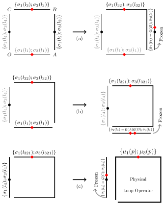
Figure 4: The $Z_{2}$ canonical transformations (18), (20), (21a) and (21b) are pictorially illustrated in (a), (b) and (c) respectively. The ${\color[rgb]{1,0,0}\blacklozenge}$ and $\bullet$ represent the electric fields of the initial horizontal and vertical links respectively.

As was done in $(1+1)$ dimensional Ising model, we glue them using canonical transformations as follows:

$$\bar{\sigma}_{3}(l_{2}) \equiv~{}~{}~{}\sigma_{3}(l_{2}), \sigma_{3}(l_{32}) \equiv\sigma_{3}(l_{3})\sigma_{3}(l_{2})$$

$$\bar{\sigma}_{1}(l_{2}) =\sigma_{1}(l_{3})\sigma_{1}(l_{2})\equiv{\cal G}(B), \sigma_{1}(l_{32}) =\sigma_{1}(l_{3}).$$ (18)

The canonical transformations (18) are illustrated in Fig. 4-a. After the transformations, the two new but equivalent canonical sets $\{\bar{\sigma}_{1}(l_{2})={\cal G}(B);\bar{\sigma}_{3}(l_{2})\}$, $\{\sigma_{1}(l_{32});\sigma_{3}(l_{32})\}$ are attached to the links $l_{2}$ and $l_{32}\equiv l_{3}l_{2}$ respectively. They satisfy the same commutation relations as the original operators (8):

$$\bar{\sigma}_{1}(l_{2})\bar{\sigma}_{3}(l_{2}) +\bar{\sigma}_{3}(l_{2})\bar{\sigma}_{1}(l_{2})=0,$$ (19)

$$\sigma_{1}(l_{32})\sigma_{3}(l_{32}) +\sigma_{3}(l_{32})\sigma_{1}(l_{32})=0.$$

One can easily check: $\bar{\sigma}_{1}^{2}(l_{2})=1,~{}\bar{\sigma}_{3}^{2}(l_{2})=1,\sigma_{1}(l_{32})^{2}=1,\sigma_{3}(l_{32})^{2}=1.$ Further, note that the two conjugate pairs $\{\bar{\sigma}_{1}(l_{2});\bar{\sigma}_{3}(l_{2})\}$ and $\{\sigma_{1}(l_{3}l_{2});\sigma_{3}(l_{3}l_{2})\}$ are also mutually independent as they commute with each other. As an example, $\left[\bar{\sigma}_{1}(l_{2}),\sigma_{3}(l_{3}l_{2})\right]\equiv\left[\sigma_{1}(l_{3})\sigma_{1}(l_{2}),\sigma_{3}(l_{3})\sigma_{3}(l_{2})\right]=0$. The new conjugate pair $\{\bar{\sigma}_{1}(l_{2});\bar{\sigma}_{3}(l_{2})\}$ is frozen due to the Gauss law at B: $\bar{\sigma}_{1}(l_{2})={\cal G}(B)\approx 1$ in ${\cal H}^{p}$. We now repeat (18) with $l_{2},l_{3}$ replaced by $l_{1},l_{32}$ respectively to define new conjugate operators $\{\bar{\sigma}_{1}(l_{1});\bar{\sigma}_{3}(l_{1})\}$ and $\{\sigma_{1}(l_{321});\sigma_{3}(l_{321})\}$ attached to the links $l_{1}$ and $l_{321}(\equiv l_{3}l_{2}l_{1})$ respectively:

$$\bar{\sigma}_{3}(l_{1})\equiv\sigma_{3}(l_{1}),~{}~{}~{}~{}~{}~{}~{}~{}~{}~{}~{}\sigma_{3}(l_{321})\equiv\sigma_{3}(l_{32})\sigma_{3}(l_{1})$$ (20)

$$~{}\bar{\sigma}_{1}(l_{1})=\sigma_{1}(l_{32})\sigma_{1}(l_{1})={\cal G}(A){\cal G}(B),~{}~{}\sigma_{1}(l_{321})=\sigma_{1}(l_{3}).$$

As before, the new conjugate pair $\{\bar{\sigma}_{1}(l_{1});\bar{\sigma}_{3}(l_{2})\}$ becomes unphysical as $\bar{\sigma}_{1}(l_{1})={\cal G}(A){\cal G}(B)\approx 1$ in ${\cal H}^{p}$. The last canonical transformations involve gluing the conjugate pairs $\{\sigma_{1}(l_{321});\sigma_{3}(l_{321})\}$ with $\{\sigma_{1}(l_{4});\sigma_{3}(l_{4})\}$ to define the dual and gauge invariant plaquette variables $\{\mu_{1}(p);\mu_{3}(p)\}$, with $p\equiv l_{1}l_{2}l_{3}l_{4}$:

$$\mu_{1}(p)\equiv\sigma_{3}(l_{321})\sigma_{3}(l_{4})\equiv\sigma_{3}(l_{3})\sigma_{3}(l_{2})\sigma_{3}(l_{1})\sigma_{3}(l_{4}).$$

$$~{}~{}~{}~{}~{}~{}~{}~{}~{}~{}~{}~{}~{}~{}\mu_{3}(p)\equiv\sigma_{1}(l_{321})~{}=\sigma_{1}(l_{3}),$$ (21a)

$$~{}~{}~{}~{}~{}~{}~{}~{}~{}~{}~{}~{}~{}~{}\bar{\sigma}_{3}(l_{4})\equiv\sigma_{3}(l_{4}),$$ (21b)

$$\bar{\sigma}_{1}(l_{4})=\sigma_{1}(l_{321})\sigma_{1}(l_{4})=\sigma_{1}(l_{3})\sigma_{1}(l_{4})\equiv{\cal G}(C).$$

To summarize, the three canonical transformations (18), (20), (21a) and (21b) transform the initial four conjugate sets $\{\sigma_{1}(l_{1});\sigma_{3}(l_{1})\}$,$\{\sigma_{1}(l_{2});\sigma_{3}(l_{2})\}$,$\{\sigma_{1}(l_{3});\sigma_{3}(l_{3})\}$, $~{}\{\sigma_{1}(l_{4});\sigma_{3}(l_{4})\}$ attached to the links $l_{1},l_{2},l_{3},l_{4}$ to four new and equivalent canonical sets $\{\bar{\sigma}_{1}(l_{2});\bar{\sigma}_{3}(l_{2})\},~{}\{\bar{\sigma}_{1}(l_{1});\bar{\sigma}_{3}(l_{1})\},~{}\{\bar{\sigma}_{1}(l_{4});\bar{\sigma}_{3}(l_{4})\}$ and $\{\mu_{1}(p);\mu_{3}(p)\}$ attached to the links $l_{2},l_{1},l_{4}$ and the plaquette $p$ respectively. The advantage of the new sets is that all the three independent Gauss law constraints at $A,B$ and $C$ are automatically solved. They freeze the three strings leaving us only with the physical spin or plaquette loop conjugate operators $\{\mu_{1}(p);\mu_{3}(p)\}$. The defining canonical relations (18), (20), (21a) and (21b) can also be inverted. The inverse transformations from the new spin flux operators to $Z_{2}$ link flux operators are

$$\sigma_{3}(l_{1})=\bar{\sigma}_{3}(l_{1}),~{}~{}~{}~{}\sigma_{3}(l_{2})=\bar{\sigma}_{3}(l_{2}),~{}~{}~{}~{}~{}~{}~{}~{}~{}~{}~{}~{}$$ (22)

$$\sigma_{3}(l_{3})=\mu_{1}(p)\bar{\sigma}_{3}(l_{4})\bar{\sigma}_{3}(l_{1})\bar{\sigma}_{3}(l_{2}),~{}~{}~{}~{}\sigma_{3}(l_{4})=\bar{\sigma}_{3}(l_{4}).$$

Similarly, the initial conjugate $Z_{2}$ electric field operators on the links are

$$\sigma_{1}(l_{1}) =\mu_{3}(p)~{}\bar{\sigma}_{1}(l_{1})=\mu_{3}(p)~{}{\cal G}(A){\cal G}(B)\approx\mu_{3}(p),$$

$$\sigma_{1}(l_{2}) =\mu_{3}(p)~{}\bar{\sigma}_{1}(l_{2})=\mu_{3}(p)~{}{\cal G}(B)\approx\mu_{3}(p)$$ (23)

$$\sigma_{1}(l_{3}) =\mu_{3}(p),$$

$$\sigma_{1}(l_{4}) =\mu_{3}(p)~{}\bar{\sigma}_{1}(l_{4})=\mu_{3}(p)~{}{\cal G}(C)\approx\mu_{3}(p).$$

Thus the complete set of gauge-spin duality relations over a plaquette and their inverses are given in (18), (20), (21a), (21b) and (22), (II.2) respectively. Note that the Gauss law constraint at the origin does not play any role as ${\cal G}(O)\approx{\cal G}(A)~{}{\cal G}(B)~{}{\cal G}(C)$. The total number of degrees of freedom also match. The initial $Z_{2}$ gauge theory had 4 spins with 3 Gauss law constraints. In the final dual spin model the 3 gauge non-invariant strings take care of the 3 Gauss law constraints leaving us with the single gauge invariant spin described by $\{\mu_{1}(p);\mu_{3}(p)\}$ on the plaquette $p$. The single plaquette $Z_{2}$ lattice gauge theory Hamiltonian (11) can now be rewritten in terms of the new gauge invariant spins as:

$$H\approx-4~{}\mu_{3}(p)-\lambda~{}\mu_{1}(p)=-\left(\begin{array}[]{ccc}\lambda{}&4\\ 4{}&-\lambda\end{array}\right).$$ (26)

Note that the equivalence of the gauge and spin Hamiltonians (11) and (26) respectively is valid only within the physical Hilbert space ${\cal H}^{p}$. The two energy eigenvalues of $H$ are $\epsilon_{\pm}=\pm 4\sqrt{\left(1+\left(\frac{\lambda}{4}\right)^{2}\right)}$.

Having discussed the essential ideas, we now directly write down the general $Z_{2}$ gauge-spin duality or canonical relations over the entire lattice. The details of these iterative canonical transformations (analogous to (18), (20), (21a) and (21b)) are given in Appendix A. Note that there are ${\cal L}$ initial spins (one on every link) with ${\cal N}$ Gauss law constraints (one at every site) satisfying the identity:

$$\prod_{(m,n)\in\Lambda}~{}{\cal G}(m,n)~{}\equiv~{}1.$$ (27)

The above identity again states that simultaneous flipping of all spins around every lattice site is an identity operator because each spin is flipped twice. As mentioned earlier, it is a property of all abelian gauge theories which reduces the number of Gauss law constraints from ${\cal N}$ to $({\cal N}-1)$. In the non-abelian SU(N) case, discussed in the next section, there is no such reduction. The global SU(N) gauge transformations, corresponding to the extra Gauss law constraints at the origin ${\cal G}^{a}(0,0)=1$, need to be fixed by hand to get the correct number of physical degrees of freedom (see section II.3.3). After canonical transformations in $Z_{2}$ lattice gauge theory, there are (a) ${\cal P}$ physical plaquette spins (analogous to $\{\mu_{1}(p);\mu_{3}(p)\}$ in the single plaquette case) shown in Figure 5-a and (b) $({\cal N}-1)$ stringy spins (analogous to $\{\bar{\sigma}_{1}(l_{1});\bar{\sigma}_{3}(l_{1})\};~{}\{\bar{\sigma}_{1}(l_{2});\bar{\sigma}_{3}(l_{2})\}$ and $\{\bar{\sigma}_{1}(l_{4});\bar{\sigma}_{3}(l_{4})\}$ in the single plaquette case) as every lattice site away from the origin can be attached to a unique string. This is shown in Figure 5-b. The degrees of freedom before and after the canonical transformations match as ${\cal L}={\cal P}+({\cal N}-1)$. All $({\cal N}-1)$ strings decouple because of the $({\cal N}-1)$ Gauss law constraints. The algebraic details of these transformations leading to freezing of all strings are worked out in detail in Appendix A.

From now onward the ${\cal P}$ physical plaquette spin/loop operators are labelled by the top right corners of the corresponding plaquettes as shown in Figure 5-a). The vertical (horizontal) stringy spin operators are labelled by the top (right) end points of the corresponding links as shown in Figure 5-b. The same notation will be used to label the dual SU(N) operators in section II.3.

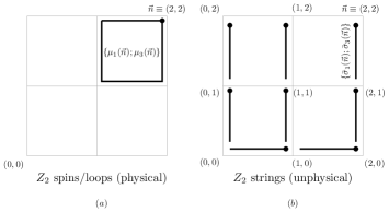
Figure 5: The physical $Z_{2}$ spin conjugate pairs $\{\mu_{1}(\vec{n});\mu_{3}(\vec{n})\}$ and the unphysical string conjugate pairs $\{\bar{\sigma}_{1}(\vec{n});\bar{\sigma}_{3}(\vec{n})\}$ dual to $Z_{2}$ lattice gauge theory are shown in (a) and (b) respectively. The co-ordinates of spin or loop operators are the co-ordinates of their top right corners. The co-ordinates of the horizontal (vertical) strings are the co-ordinates of their right (top) end points. These are shown by $\bullet$ in (a) and (b). The strings decouple from the physical Hilbert space as $\bar{\sigma}_{1}(\vec{n})={\cal G}(\vec{n})\approx 1$ by Gauss law constraint at $\vec{n}$. The corresponding dual SU(N) spin and SU(N) string operators are shown in Figure 10-a,b respectively.

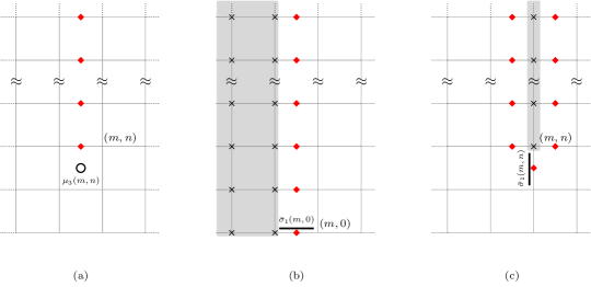
Figure 6: The non-local relations in the $Z_{2}$ gauge-spin duality transformations: (a) shows the relations (28b) expressing $\mu_{3}(m,n)$ as the product of $\sigma_{1}$ operators denoted by $\blacklozenge$. In (b) and (c), we show the relations (30b) expressing $\bar{\sigma}_{1}(m,0)$ and $\bar{\sigma}_{1}(m,n);~{}n\neq 0$ respectively as the product of $\sigma_{1}$ operators denoted by $\blacklozenge$. As $\sigma_{1}^{2}=1$, the string operators $\bar{\sigma}_{1}(m,0)$ and $\bar{\sigma}_{1}(m,n)$ are also a product of Gauss law operators at sites marked by x in the shaded regions. For similar SU(N) relations, see Figures 11.

II.2.1 Physical sector and $Z_{2}$ dual potentials

The final duality relations between the initial conjugate sets $\{\sigma_{1}(m,n;\hat{i});\sigma_{3}(m,n;\hat{i})\}$ on every lattice link $(m,n;\hat{i})$ and the final physical conjugate loop operators $\{\mu_{1}(m,n)$; $\mu_{3}(m,n)\}$ are (see Appendix A)

$$\mu_{1}(m,n) =\sigma_{3}(m-1,n-1;\hat{1})~{}\sigma_{3}(m-1,n-1;\hat{2})$$

$$~{}~{}~{}~{}~{}~{}~{}~{}\sigma_{3}(m,n;-\hat{2})\sigma_{3}(m,n;-\hat{1}),$$ (28a)

$$\mu_{3}(m,n)=\prod\limits_{n^{\prime}=n}^{N}\sigma_{1}(m-1,n^{\prime};\hat{1}).$$ (28b)

In (28a) we have defined $\sigma_{1}(m,n;-\hat{1})\equiv\sigma_{1}(m-1,n;\hat{1})$ and $\sigma_{1}(m,n;-\hat{2})\equiv\sigma_{1}(m,n-1;\hat{2})$. The relations (28a) and (28b) are the extension of the single plaquette relations (21a) to the entire lattice. They are illustrated in Figure 6-a. The canonical commutation relations are

$$\mu_{1}(m,n)\mu_{3}(m,n)+\mu_{3}(m,n)\mu_{1}(m,n)=0.$$ (29)

Further, $\mu_{3}(m,n)^{2}=1,\mu_{1}(m,n)^{2}=1$. The canonical transformations (28a) are important as they define the magnetic field operators $\mu_{1}(m,n)$ and its conjugate $\mu_{3}(m,n)$ as a new dual fundamental operators. The electric field is derived from the electric scalar potentials. This should be contrasted with the original description where electric fields $\sigma_{1}(m,n)$ were fundamental and the magnetic fields were derived from the magnetic magnetic vector potentials as $\sigma_{3}(l_{1})\sigma_{3}(l_{2})\sigma_{3}(l_{3})\sigma_{3}(l_{4})$.

II.2.2 Unphysical sector and $Z_{2}$ string operators

The unphysical string conjugate pair operators are (see Appendix A)

$$\bar{\sigma}_{3}(m,0) =\sigma_{3}(m-1,0;\hat{1}),$$

$$\bar{\sigma}_{3}(m,n) =\sigma_{3}(m,n-1;\hat{2});~{}~{}~{}~{}n\neq 0$$ (30a)

$$\bar{\sigma}_{1}(m,0) =\prod\limits_{m^{\prime}=0}^{m-1}\prod\limits_{n^{\prime}=0}^{N}{\cal G}(m^{\prime},n^{\prime})\approx 1,$$

$$\bar{\sigma}_{1}(m,n) =\prod\limits_{n^{\prime}=n}^{N}{\cal G}(m,n^{\prime})\approx 1;~{}~{}~{}~{}n\neq 0.$$ (30b)

The relations (30a) and (30b) are illustrated in Figure 6-b and Figure 6-c respectively. It is easy to see that in the full gauge theory Hilbert space $\bar{\sigma}_{1}(m,n)\bar{\sigma}_{3}(m,n)+\bar{\sigma}_{3}(m,n)\bar{\sigma}_{1}(m,n)=0$ and different string operators located at different lattice sites commute with each others. Further, one can check that all strings and plaquette operators are mutually independent and commute with each other:

$$\left[\mu_{3}(m,n),\bar{\sigma}_{1}(m^{\prime},n^{\prime})\right]=0,\left[\mu_{3}(m,n),\bar{\sigma}_{3}(m^{\prime},n^{\prime})\right]=0,$$ (31)

$$\left[\mu_{1}(m,n),\bar{\sigma}_{1}(m^{\prime},n^{\prime})\right]=0,\left[\mu_{1}(m,n),\bar{\sigma}_{3}(m^{\prime},n^{\prime})\right]=0.$$

II.2.3 Inverse relations

The inverse relations for the flux operators over the entire lattice are

$$\sigma_{3}(m,0;\hat{1}) =\bar{\sigma}_{3}(m+1,0),$$

$$\sigma_{3}(m,n;\hat{2}) =\bar{\sigma}_{3}(m,n+1)$$

$$\sigma_{3}(m,n;\hat{1}) =\bigg{(}\prod\limits_{l=1}^{n}\bar{\sigma}_{3}(m,l)\bigg{)}\bigg{(}\prod\limits_{q=1}^{n}\bar{\sigma}_{3}(m+1,q)\bigg{)}$$

$$~{}~{}~{}~{}~{}~{}~{}~{}~{}\bigg{(}\prod\limits_{p=1}^{n}{\mu}_{1}(m+1,p)\bigg{)};~{}~{}n\neq 0$$ (32)

On the other hand, the conjugate electric field operators are

$$\sigma_{1}(m,n;\hat{1})=\mu_{3}(m,n)\mu_{3}(m,n+1),~{}~{}~{}~{}~{}~{}$$

$$\sigma_{1}(m,n;\hat{2})=\mu_{3}(m,n+1)\mu_{3}(m+1,n+1).$$ (33)

In the second relation in (II.2.3), we have used Gauss laws at $(m,l)~{};l=n+1,n+2,\cdots$. The above relations are analogous to the inverse relations (22) and (II.2) in the single plaquette case.

II.2.4 $Z_{2}$ Gauss laws & solutions

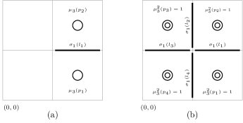
Figure 7: (a) shows the $Z_{2}$ link electric field operator $\sigma_{1}(m,n;\hat{1})$ as the product of nearest neighbor loop operators $\mu_{3}(p_{1})$ and $\mu_{3}(p_{2})$, (b) graphically illustrates how the spin or electric potential operators $\{\mu_{3}(p_{1}),\mu_{3}(p_{2}),\mu_{3}(p_{3}),\mu_{3}(p_{4})\}$ solve the $Z_{2}$ Gauss law (35) at site $(m,n)$. A similar SU(N) proof is involved and given in Appendix B.1.

It is easy to see that the Gauss law constraints are automatically satisfied by the dual spin operators as shown in Figure 7-a,b. We write the $Z_{2}$ electric fields around a site $(m,n)$ in terms of the electric scalar potentials:

$$\sigma_{1}(l_{1})\equiv\sigma_{1}(m,n;\hat{1})=\mu_{3}(p_{1})\mu_{3}(p_{2}),$$

$$\sigma_{1}(l_{2})\equiv\sigma_{1}(m,n;\hat{2})=\mu_{3}(p_{2})\mu_{3}(p_{3}),$$

$$\sigma_{1}(l_{3})\equiv\sigma_{1}(m-1,n;\hat{1})=\mu_{3}(p_{3})\mu_{3}(p_{4}),$$

$$\sigma_{1}(l_{4})\equiv\sigma_{1}(m,n-1;\hat{2})=\mu_{3}(p_{4})\mu_{3}(p_{1}).$$ (34)

In (34) we have used link and plaquette labels from Figure 7. As $\mu_{3}^{2}(p)=1$, we get

$${\cal G}(m,n) =\sigma_{1}(l_{1})\sigma_{1}(l_{2})\sigma_{1}(l_{3})\sigma_{1}(l_{4})\equiv 1.$$ (35)

The above duality property also generalizes to the SU(N) case. The dual SU(N) spin operators or potentials are the solutions of local SU(N) Gauss laws at all the sites except origin. However, unlike the trivial cancellations above, the non-abelian cancellations are highly nontrivial and are worked out in detail in Appendix B.1.

II.2.5 $Z_{2}$ dual dynamics

The $Z_{2}$ lattice gauge theory Hamiltonian (11) in terms of the physical spin operators takes the simple nearest neighbor interaction form:

$$H=-\sum_{<p,pm,n>}\mu_{3}(p)\mu_{3}(p^{\prime})-\lambda\sum\limits_{p}\mu_{1}(p)\equiv H_{E}+\lambda H_{B},$$

$$~{}~{}~{}~{}~{}~{}=\lambda\bigg{[}-\sum\limits_{p}\mu_{1}(p)-\frac{1}{\lambda}\sum\limits_{<p,p^{\prime}>}\mu_{3}(p)\mu_{3}(p^{\prime})\bigg{]}$$ (36)

In (36) $\sum_{<p,p^{\prime}>}$ denotes the sum over the nearest neighbor plaquettes. Note that the original fundamental non-interacting electric field terms are now described by nearest neighbor interacting electric scalar potentials. The non-interacting magnetic fields, on the other hand, have now acquired the fundamental status. Thus the two gauge-spin descriptions:

$$\{\sigma_{1}(l);\sigma_{3}(l)\}\leftrightarrow\{\mu_{1}(p);\mu_{3}(p)\}$$

are related by duality. Further, $Z_{2}$ lattice gauge theory at coupling $\lambda$ is mapped into $Z_{2}$ spin model at coupling $(1/\lambda)$, i.e,

$$H^{{}^{Z_{2}}}_{gauge}(\lambda)\simeq\lambda~{}H^{{}^{Z_{2}}}_{spin}({1}/{\lambda}).$$

We have used $\simeq$ above to emphasizes that this equivalence is only within the physical Hilbert space ${\cal H}^{p}$.

II.2.6 $Z_{2}$ Magnetic disorder operator

The dual spin model (36) on an infinite lattice has global $Z_{2}$ invariance:

$$\mu_{1}(p)\rightarrow\mu_{1}(p),~{}~{}~{}~{}\mu_{3}(p)\rightarrow-\mu_{3}(p),~{}~{}\forall p\in\Lambda.$$ (37)

Its generator ${G}_{\Lambda}\equiv\prod\limits_{p\in\Lambda}\mu_{1}(p)$ leaves the Hamiltonian (36) invariant: ${G}_{\Lambda}H{G}^{-1}_{\Lambda}=H$. Unlike the initial $Z_{2}$ gauge symmetry of $Z_{2}$ gauge theory, the global $Z_{2}$ symmetry of the dual spin model (36) is the symmetry of the spectrum. Being independent of gauge invariance, it allows the Ising spin model (36) to be magnetized through spontaneous symmetry breaking for $\lambda<<1$. As a consequence of duality:

$$\Big{<}\mu_{1}(p)\Big{>}_{{}_{H^{z_{2}}_{spin}({1}/{\lambda})}}=\Big{<} \sigma_{3}(l_{1})\sigma_{3}(l_{2})\sigma_{3}(l_{3})\sigma_{3}(l_{4})\Big{>}_{{}_{H^{z_{2}}_{gauge}(\lambda)}}$$

$$\Big{<}\mu_{3}(m,n)\Big{>}_{H^{z_{2}}_{spin}(1/\lambda)} =\left<\prod_{n^{\prime}=n}^{N}\sigma_{1}(m,n^{\prime})\right>_{H^{z_{2}}_{gauge}(\lambda)}$$ (38)

Figure 8: Duality and order, disorder in (a) $(2+1)$ dimensional $Z_{2}$ lattice gauge theory, (b) $(2+1)$ dimensional Ising model. The confining ($\lambda<<1$) and deconfining ($\lambda>>1$) phases of $Z_{2}$ lattice gauge theory correspond to the ferromagnetic and paramagnetic phases of the Ising spin model kogrev ; fradsuss ; horn ; savit .

The above two equations describe the relationship between order and disorder in the gauge and the dual spin system. Note that we always measure order or disorder with respect to the potentials. The first relation above states that at low temperature or large coupling $\lambda>>1$, the gauge system is in ordered phase. This is because all magnetic vector potentials $(\sigma_{3}(l))$ are aligned (close to unity) leading to $\sigma_{3}(l_{1})\sigma_{3}(l_{2})\sigma_{3}(l_{3})\sigma_{3}(l_{4})\approx 1$. This is the free phase of $Z_{2}$ gauge theory mentioned in the introduction with Wilson loop following perimeter law:

$$\langle W_{[{\cal C}]}\rangle\equiv\langle\prod_{l\in{\cal C}}\sigma_{3}(l)\rangle=exp\Big{(}-{\lambda}^{-2}~{}{\textrm{P}erimeter}{({\cal C})}\Big{)},$$

$$\hskip 56.9055pt\lambda>>1.$$ (39)

However, the dual spin system is now at high temperature. It is in the disordered phase as the dual electric scalar potential or the spin values $\mu_{3}(p)=\pm 1$ are equally probable. On the other hand, at small coupling ($\lambda<<1$), the spin system is ordered with all electric scalar potentials aligned to the value $\mu_{3}(p)=+1$ or $-1$. The gauge system is now disordered as the two values of the magnetic vector potentials $\sigma_{3}(l)=\pm 1$ are equally probable. This is the confining phase with the $Z_{2}$ Wilson loop $W_{[{\cal C}]}$ around a closed curve ${\cal C}$ following the area law:

$$\langle W_{[{\cal C}]}\rangle\equiv\langle\prod_{l\in{\cal C}}\sigma_{3}(l)\rangle\sim\left({\lambda}\right)^{Area({\cal C})}=exp\Big{(}-|ln\lambda|~{}{\textrm{A}rea}{({\cal C})}\Big{)},$$

$$\hskip 56.9055pt\lambda<<1.$$ (40)

Figure 9: Duality between SU(N) lattice gauge theory and an SU(N) spin model. Unlike the corresponding $Z_{2}$ duality in Figure 3-a,b, global SU(N) Gauss law constraints at the origin remain unsolved due to the non-abelian nature of the gauge transformations.

The disorder in the gauge system is the order in the dual spin system which is measured by the expectation value of electric scalar potential $\mu_{3}(p)$. It is a (non-local) product of the original link electric fields which flip the magnetic vector potentials $\sigma_{3}(l)$ along an infinite path. This is shown in Figure 6-a. For latter convenience and comparisons with SU(N) results, the $Z_{2}$ disorder operator is relabeled as:

$${\Sigma}(m,n)\equiv\mu_{3}(m,n)=\prod_{n^{\prime}=n}^{N}~{}\sigma_{1}(m,n^{\prime}).$$ (41)

Just like in the case of Kramers-Wannier duality km ; fradsuss ; kogrev ; horn , the disorder operator $\Sigma(m,n)$ in $Z_{2}$ gauge theory acting on an ordered state creates a kink state fradsuss ; kogrev which is orthogonal to the original ordered state. Note that a kink at plaquette $p$ is a magnetic vortex at $p$ in the original gauge language. Therefore the expectation value of the disorder operator in an ordered state (no kinks or vortices) is $0$. Below the critical point $\lambda_{c}$, its expectation value is non-zero. This is the disordered phase and can be understood in terms of kink or magnetic vortex condensation kogrev . We therefore obtain:

$$\left<\Sigma(m,n)\right>\neq 0~{}~{}~{}~{}~{}~{}~{}~{}~{}~{}~{}~{}~{}~{}\lambda<<1,$$

$$\left<\Sigma(m,n)\right>=0~{}~{}~{}~{}~{}~{}~{}~{}~{}~{}~{}~{}~{}~{}\lambda>>1.$$ (42)

The $Z_{2}$ gauge-spin duality and the phase diagrams are shown in Figure 8. Note that the disorder operator $\Sigma(m,n)$ is gauge invariant as it commutes with the local Gauss law operators ${\cal G}(n)$. We further define $\mu_{3}(m,n)\equiv e^{i\pi{\cal E}(m,n)}$. Using (9), we get:

$${\Sigma}(m,n)=~{}~{}exp{~{}i\Big{(}\tiny{\pi~{}{\cal E}(m,n)}\Big{)}}=$$

$$exp~{}i\Big{(}\pi\footnotesize{\sum_{n^{\prime}=n}^{N}E(m,n^{\prime};\hat{1})}\Big{)}\equiv{\Sigma}_{\pi}(m,n).$$ (43)

The order-disorder algebra is obtained by using the anti-commutation relation between $\sigma_{1}(l)$ and $\sigma_{3}(l)$:

$$W_{[{\cal C}]}~{}\Sigma_{\pi}(m,n)=\left(-1\right)^{q}~{}\Sigma_{\pi}(m,n)~{}W_{[{\cal C}]}.$$ (44)

As ${\cal C}$ is a closed loop: $q=1$ if the point $(m,n)$ is inside ${\cal C}$ and $q=0$ if $(m,n)$ is outside ${\cal C}$. This can be generalized to more complicated curves where $q$ equals the winding number which is the number of times the curve ${\cal C}$ winds around the plaquette at $(m,n)$. The algebra (44) is the standard Wilson-’t Hooft loop algebra for the simplest $Z_{2}$ lattice gauge theory in $(2+1)$ dimensions. In the next section, we construct SU(N) duality transformations and exploit them to generalize (43) and (44) to SU(N) lattice gauge theory.

II.3 SU(N) duality and SU(N) Spin Model

In this section, we construct SU(N) spin model which is dual to SU(N) lattice gauge theory. As mentioned earlier, dualities in abelian, non-abelian lattice gauge theories have been extensively studied in the past thmds ; hooft ; banks ; fradsuss ; kogrev ; savit ; horn ; sharatram ; manu . Most of these studies involve path integral approach and abelian gauge groups. The duality transformations are used to make the compactness of the abelian and non-abelian gauge groups manifest in the form of topological (magnetic monopoles) degrees of freedom banks . Our purpose in this section is to show that SU(N) lattice gauge theory can be constructively dualized like $Z_{2}$ lattice gauge theory in the previous section. This is illustrated in Figure 9. The SU(N) dual (spin) operators also lead to a new SU(N) disorder operator discussed in section II.3.6. We directly motivate the SU(N) results through the $Z_{2}$ lattice gauge theory duality discussed in the previous section. All algebraic details of SU(N) canonical transformations can be found in msprd . For the sake of comparison and convenience, all initial and final dual spin operators involved in $Z_{2}$ and $SU(N)$ lattice gauge theories are shown in Table-1. The abelian $U(1)$ results can be easily obtained by ignoring all non-abelian terms from the duality transformations at the end.

The basic operators involved in the Kogut-Susskind Hamiltonian formulation of SU(N) lattice gauge theories are $SU(N)$ flux operators $U(\vec{n};\hat{i})$ and the corresponding left, right electric fields $E^{a}_{+}(\vec{n};\hat{i})$ and $E^{a}_{-}(\vec{n}+\hat{i};\hat{i})$ and on every link ks . They satisfy the following canonical commutation relations:

$$\left[E^{a}_{+}(\vec{n};\hat{i}),U_{\alpha\beta}(\vec{n};\hat{i})\right]=-\left(\frac{\lambda^{a}}{2}U(\vec{n};\hat{i})\right)_{\alpha\beta},$$

$$\left[E^{a}_{-}(\vec{n}+\hat{i};\hat{i}),U_{\alpha\beta}(\vec{n};\hat{i})\right]=\left(U(\vec{n};\hat{i})\frac{\lambda^{a}}{2}\right)_{\alpha\beta}$$ (45a)

$$\left[E^{a}_{+}(\vec{n};\hat{i}),E^{b}_{+}(\vec{n};\hat{i})\right]=if^{abc}E^{c}_{+}(\vec{n};\hat{i}),$$

$$\left[E^{a}_{-}(\vec{n};\hat{i}),E^{b}_{-}(\vec{n};\hat{i})\right]=if^{abc}E^{c}_{-}(\vec{n};\hat{i}).$$ (45b)

In (45a) and (45b), $\lambda^{a}(a=1,2,\cdots,N^{2}-1)$ are the representation matrices in the fundamental representation of SU(N) satisfying $Tr\left(\lambda^{a}\lambda^{b}\right)=\frac{1}{2}\delta^{ab}$ and $f^{abc}$ are the SU(N) structure constants. $E_{-}^{a}(\vec{n}+\hat{i};\hat{i})$ and $E_{+}^{a}(\vec{n};\hat{i})$ are the generators of right and left gauge transformations on the link flux operator $U(\vec{n};\hat{i})$. The left and the right electric fields are not independent and are related by:

$$E_{-}^{a}(\vec{n}+\hat{i};\hat{i})=-R_{ab}(U^{\dagger}(\vec{n};\hat{i}))E_{+}^{b}(\vec{n};\hat{i});$$

$$~{}~{}~{}~{}R_{ab}(U(\vec{n};\hat{i}))\equiv\frac{1}{2}Tr\left(\lambda^{a}U(\vec{n};\hat{i})\lambda^{b}U^{\dagger}(\vec{n};\hat{i})\right).$$ (46)

The rotation operator R satisfies $R^{T}R=RR^{T}=1$. The local SU(N) gauge transformations rotate the link operators and the electric fields as:

$$E_{\pm}(\vec{n};\hat{i})\rightarrow\Lambda(\vec{n})~{}E_{\pm}(\vec{n};\hat{i})~{}\Lambda^{\dagger}(\vec{n}),$$

$$U(\vec{n};\hat{i})\rightarrow\Lambda(\vec{n})~{}U(\vec{n};\hat{i})~{}\Lambda^{\dagger}(\vec{n}+\hat{i})$$ (47)

the generators of SU(2) gauge transformations at any lattice site n are:

$${\cal G}^{a}(\vec{n})=\sum_{i=1}^{d=2}\Big{(}E_{-}^{a}(\vec{n};\hat{i})+E_{+}^{a}(\vec{n};\hat{i})\Big{)},~{}~{}~{}~{}~{}~{}~{}\forall~{}~{}\vec{n},~{}a.$$ (48)

Therefore there is a Gauss law constraint ${\cal G}^{a}(\vec{n})|\psi\rangle_{phys}=0$ at each lattice site $\vec{n}$, where $|\psi\rangle_{phys}$ is any physical state. The Hamiltonian is

$$H =\frac{g^{2}}{2}\sum\limits_{l}E^{a}(l)E^{a}(l)+\frac{1}{2g^{2}}\sum\limits_{p}\Big{(}2N-\left(Tr~{}U_{p}+h.c\right)\Big{)}$$

$$~{}~{}~{}~{}~{}~{}~{}~{}~{}~{}~{}~{}~{}~{}~{}\equiv~{}\left(g^{2}H_{E}+\frac{1}{g^{2}}H_{B}\right).$$ (49)

Above, $l$ and $p$ refer to links and plaquettes on the lattice. $U_{p}$ is the product of link operators corresponding to the links along a plaquette. $g^{2}$ is the coupling constant. Like in $Z_{2}$ gauge theory Hamiltonian (11), all interactions are contained in the magnetic part $H_{B}$ of the Hamiltonian. The electric part $H_{E}$, with no interactions, can be easily diagonalized leading to gauge invariant strong coupling expansion in terms of loop states ks ; manu . After duality in the next section, like $Z_{2}$ lattice gauge theory in section II.2.5, their roles will be reversed.

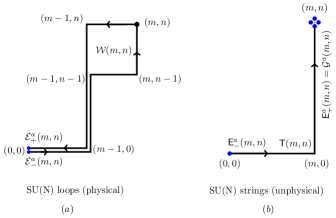
Figure 10: The physical SU(N) spin conjugate pairs $\{{\cal E}_{\pm};{\cal W}_{\alpha\beta}\}$ and the unphysical SU(N) string conjugate pairs $\{{\sf E}_{\pm}(n);{\sf T}(n)\}$ dual to SU(N) lattice gauge theory are shown in (a) and (b) respectively. Like in $Z_{2}$ case in Figure 5, we label the SU(N) spin operators by their top right corners and the SU(N) string operators by their endpoints. The strings decouple from the physical Hilbert space as ${\sf E}_{+}^{a}(m,n)\approx 0$ by the Gauss law constraints in ${\cal H}^{p}$.

II.3.1 Physical sector and SU(N) dual potentials

$Z_{2}$ lattice gauge theory		SU(N) lattice gauge theory
Gauge Operators	Dual/Spin Operators	Gauge Operators	Dual/Spin Operators
	$\left\{\mu_{1}(m,n);\mu_{3}(m,n)\right\}$		$\left\{{\cal E}_{\pm}^{a}(m,n);~{}{\cal W}_{\alpha\beta}(m,n)\right\}$
	($Z_{2}$ Loops/$Z_{2}$ Ising spins)		(SU(N) Loops/SU(N) spins)
$\left\{\sigma_{1}(m,n;\hat{i});\sigma_{3}(m,n;\hat{i})\right\}$		$\left\{E_{\pm}^{a}(m,n;\hat{i});U_{\alpha\beta}(m,n;\hat{i})\right\}$
	$\left\{\bar{\sigma}_{1}(m,n);\bar{\sigma}_{3}(m,n)\right\}$		$\left\{{\sf E}_{\pm}^{a}(m,n);~{}{\sf T}_{\alpha\beta}(m,n)\right\}$
	(Frozen $Z_{2}$ Strings)		(Frozen $SU(N)$ Strings)

Table 1: The basic conjugate operators of the original and the dual $Z_{2}$, SU(N) gauge theories in $(2+1)$ dimensions.

We now define the dual SU(N) spin and SU(N) string operators analogous to the $Z_{2}$ spins and strings in (28a), (28b) and (30a), (30b) respectively. They are pictorially described in Figure 10-a,b respectively. Due to the non-abelian nature of the electric field and the flux operators, the SU(N) duality relations have additional non-abelian structures msprd . To begin with, the ${\cal N}$ SU(N) Gauss law constraints at ${\cal N}$ different lattice sites are all mutually independent. In other words, identities like (27) do not exist. As a result, there is a global SU(N) invariance in the SU(N) spin model corresponding to the gauge transformations at the origin. All dual operators transform covariantly under this global SU(N). As shown in Figure 10, the SU(N) duality transformations involve parallel transports from the origin to the site of the dual operators. The string flux operator ${\sf T}(m,n)$ at a lattice site $(m,n)$ (analogous to $\bar{\sigma}_{3}(m,n)$ in the $Z_{2}$ case) is defined through the path $(0,0)\rightarrow(m,0)\rightarrow(m,n)$:

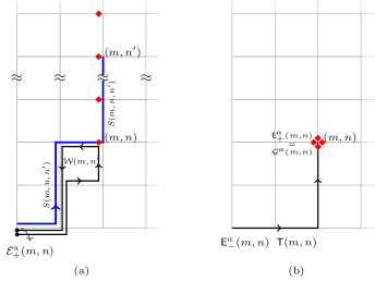
Figure 11: The non-local relations in SU(N) duality transformations and the Gauss law constraints. (a) We show the relations (51b) expressing ${\cal E}_{+}^{a}(m,n)$ as the sum of $E_{-}^{b}(m,n^{\prime};\hat{1})$. The Kogut-Susskind electric fields and and the plaquette loop electric fields are denoted by $\blacklozenge$ and $\bullet$ respectively. In (b) we show the SU(N) Gauss law constraints (57). The corresponding $Z_{2}$ illustrations are in Figure 6-a,b,c.

$${\sf T}(m,n)=\left(\prod_{m^{\prime}=0}^{m}U(m^{\prime},0;\hat{1})\prod_{n^{\prime}=0}^{n}U(m,n^{\prime};\hat{2})\right),$$ (50a)

$${\sf E}^{a}_{+}(m,n)={\cal G}^{a}(m,n)\approx 0,$$ (50b)

These strings and their electric fields ${\sf E}^{a}_{+}(m,n)$ are shown in Figure 10-b and Figure 11-b respectively. The relations (50a) and (50b) are the SU(N) analogues of the $Z_{2}$ string relations (30a) and (30b) respectively. The dual SU(N) spin and the SU(N) electric scalar potential operators in terms of the original Kogut-Susskind operators are defined msprd as

$${\mathcal{W}}(m,n) ={\sf T}(m-1,n-1)~{}U_{p}(m,n)~{}{\sf T}^{\dagger}(m-1,n-1),$$ (51a)

$${\mathcal{E}}_{+}^{a}(m,n) =\sum\limits_{n^{\prime}=n}^{\sf N}R_{ab}(S(m,n;n^{\prime}))E_{-}^{b}(m,n^{\prime};\hat{1}).$$ (51b)

The two operators in (51a) and (51b) are the non-abelian extensions of the two $Z_{2}$ dual operators defined in (28a) and (28b) respectively. In (51a), (51b), the plaquette operator $U_{p}(m,n)$ and the parallel transport $S(m,n;n^{\prime})$ are defined as

$$U_{p}(m,n)=U(m-1,n-1;\hat{1})~{}U(m,n-1;\hat{2})$$

$$~{}~{}~{}~{}~{}~{}~{}~{}U^{\dagger}(m-1,n;\hat{1})~{}U^{\dagger}(m-1,n-1;\hat{2}),$$ (52)

$$S(m,n;n^{\prime})\equiv{\sf T}(m-1,n)~{}U(m-1,n;\hat{1})~{}\prod_{q=n}^{n^{\prime}}~{}U(m,q;\hat{2}).$$

The relation (51a) defines the SU(N) magnetic field operator as a fundamental operator. The second relation (51b) defines SU(N) electric scalar potential ${\cal E}^{a}(m,n)$ which is dual to the original magnetic vector potential. The appearance of the ${\sf T}(m,n)$ and $S(m,n;n^{\prime})$ in (51a) ad (51b) is due to the non-abelian nature of the operators. These parallel transports from the origin are required to have consistent gauge transformation properties of the SU(N) magnetic fields and the SU(N) electric scalar potentials (see (58)).

The dual or loop operators satisfy the expected non-abelian duality or quantization rules:

$$\left[{\cal E}^{a}_{-}(m,n),{\cal W}_{\alpha\beta}(m,n)\right] =-\left(\frac{\lambda^{a}}{2}{\cal W}(m,n)\right)_{\alpha\beta},$$

$$\left[{\cal E}^{a}_{+}(m,n),{\cal W}_{\alpha\beta}(m,n)\right] =\left({\cal W}(m,n)\frac{\lambda^{a}}{2}\right)_{\alpha\beta},$$ (53a)

$$\left[{\cal E}^{a}_{-}(m,n),{\cal E}_{-}^{b}(m,n)\right] =if^{abc}{\cal E}^{c}_{-}(m,n),$$

$$\left[{\cal E}^{a}_{+}(m,n),{\cal E}_{+}^{b}(m,n)\right] =if^{abc}{\cal E}^{c}_{+}(m,n).$$ (53b)

Further, the two electric fields are related through parallel transport and commute:

$${\cal E}_{-}^{a}(m,n)\equiv-R_{ab}({\cal W}^{\dagger}(m,n)){\cal E}_{+}^{b}(m,n)$$

$$=>\left[{\cal E}^{a}_{-}(m,n),{\cal E}^{b}_{+}(m,n)\right]=0.$$ (54)

The quantization relations (53a), (53b) and (54) are exactly similar to the original quantization rules (45a) and (45b) respectively. Thus the electric field operator $E^{a}(m,n;\hat{i})$ and the magnetic vector potential operator $U_{\alpha\beta}(m,n;i)$ have been replaced by their dual electric scalar potential ${\cal E}^{a}(m,n)$ and the dual magnetic field operator ${\cal W}_{\alpha\beta}(m,n)$. This is similar to $Z_{2}$ lattice gauge theory duality where $\{\sigma_{1}(m,n);\sigma_{3}(m,n)\}$ get replaced by $\{\mu_{3}(m,n);\mu_{1}(m,n)\}$. We again emphasize that ${\cal E}^{a}(m,n)$ defines the dual electric scalar potential as it is conjugate to the fundamental magnetic flux operator ${\cal W}_{\alpha\beta}(m,n)$.

II.3.2 Unphysical sector and SU(N) string operators

The unphysical sector, representing the gauge degrees of freedom, consists of the string flux operators ${\sf T}(m,n)$ in (50a) and their conjugate electric fields ${\sf E}^{a}(m,n)$ in (50b). They satisfy the canonical quantization relations:

$$\left[{\sf E}^{a}_{-}(m,n),{\sf T}_{\alpha\beta}(m,n)\right] =-\left(\frac{\lambda^{a}}{2}{\sf T}(m,n)\right)_{\alpha\beta},$$

$$\left[{\sf E}^{a}_{+}(m,n),{\sf T}_{\alpha\beta}(m,n)\right] =\left({\sf T}(m,n)\frac{\lambda^{a}}{2}\right)_{\alpha\beta}$$ (55a)

$$\left[{\sf E}^{a}_{-}(m,n),{\sf E}_{-}^{b}(m,n)\right] =if^{abc}{\sf E}^{c}_{-}(m,n),$$

$$\left[{\sf E}^{a}_{+}(m,n),{\sf E}_{+}^{b}(m,n)\right] =if^{abc}{\sf E}^{c}_{+}(m,n).$$ (55b)

Again, the operators ${\sf T}_{+}^{a}$ and ${\sf T}_{-}^{b}$ are related through parallel transport and commute amongst themselves:

$$~{}~{}{\sf E}_{-}^{a}(m,n)\equiv-R_{ab}({\sf T}^{\dagger}(m,n)){\sf E}_{+}^{b}(m,n)$$

$$=>~{}~{}\left[{\sf E}^{a}_{-}(m,n),{\sf E}^{b}_{+}(m,n)\right]=0.$$ (56)

The right string electric fields are

$${\sf E}^{a}_{+}(m,n) =\sum_{i=1}^{2}\left[E^{a}_{-}(m,n;\hat{i})+E^{a}_{+}(m,n;\hat{i})\right]$$ (57)

$$={\cal G}^{a}(m,n)\approx 0,~{}~{}\forall(m,n)\neq(0,0).$$

Thus as in $Z_{2}$ lattice gauge theory, the SU(N) Gauss law constraints freeze all SU(N) string degrees of freedom. This is shown in Figure 10-b. As a consequence, all strings (or gauge degrees of freedom) completely decouple from the theory.

II.3.3 The residual Gauss law

Unlike $Z_{2}$ lattice gauge theory, the SU(N) Gauss law at the origin is independent of the SU(N) Gauss laws at other sites. In other words, the abelian identity (27) has no non-abelian analogue. Under this residual global gauge invariance at the origin $\Lambda\equiv\Lambda(0,0)$, all loop operators transform like adjoint matter fields:

$${\cal E}_{\pm}(p)\rightarrow\Lambda~{}{\cal E}_{\pm}(p)~{}\Lambda^{\dagger},~{}~{}~{}{\cal W}(p)\rightarrow\Lambda~{}{\cal W}(p)~{}\Lambda^{\dagger}.$$ (58)

Above, ${\cal E}_{\pm}(p)\equiv{\cal E}_{\pm}(m,n),{\cal W}(p)\equiv{\cal W}(m,n)$ and $\Lambda\equiv\Lambda(0,0)$ is the gauge transformation at the origin. This global invariance at the origin is fixed by the $(N^{2}-1)$ global SU(N) Gauss laws:

$$~{}{\cal G}^{a}\equiv{\cal G}^{a}(0,0)=E^{a}_{+}(0,0;\hat{1})+E^{a}_{-}(0,0;\hat{2})$$

$$=\sum_{m=1}^{\sf N}\sum_{n=1}^{\sf N}\left[\underbrace{{\sf E}^{a}_{-}(m,n)}_{=0}+\underbrace{{\cal E}^{a}_{+}(m,n)+{\cal E}^{a}_{-}(m,n)}_{\equiv{\mathbb{L}}^{a}(m,n)}\right]$$

$$~{}~{}~{}~{}~{}~{}~{}~{}\equiv\sum_{m=1}^{\sf N}\sum_{n=1}^{\sf N}{\mathbb{L}}^{a}(m,n)=0.$$ (59)

In (59), the total left and right electric flux operators on a plaquette located at $p=(m,n)$ are donated by ${\mathbb{L}}^{a}(m,n)$ and equations (56), (57) are used to get ${\sf E}^{a}_{-}(m,n)=0$. In Appendix B.1 we show that the dual SU(N) electric scalar potentials, like $Z_{2}$ electric potentials in (35), solve the SU(N) Gauss law constraints away from the origin and lead to (59) at the origin. The residual global constraints (59) can be solved by using the angular momentum or spin network basis sharatram ; manu ; msplb ; msprd . Note that in the abelian U(1) case there is no residual Gauss law as ${\mathbb{L}}^{a}(m,n)\rightarrow{\mathbb{L}}(m,n)\equiv{\cal E}_{+}(m,n)+{\cal E}_{-}(m,n)\equiv 0$.

II.3.4 Inverse relations

The inverse flux operator relations, analogous to the $Z_{2}$ relations (32), are

$$U(m,n;\hat{1})={\sf T}^{\dagger}(m,n)~{}{\cal W}(m+1,n)~{}{\cal W}(m+1,n-1)\cdot$$

$$\cdots{\cal W}(m+1,1)~{}{\sf T}(n+1,y),~{}~{}~{}~{}~{}~{}~{}~{}~{}$$

$$U(m,n;\hat{2})=~{}T(m,n+1)~{}T^{\dagger}(m,n).\hskip 56.9055pt$$ (60)

The inverse electric field relations, analogous to the $Z_{2}$ electric field relations (II.2.3), are

$$E_{+}^{a}(m,n;\hat{1})=R_{ab}({\sf T}(m,n))\bigg{\{}{\cal E}_{-}^{b}(m+1,n+1)~{}~{}~{}~{}~{}~{}~{}$$

$$+~{}{\cal E}_{+}^{b}(m+1,n)+\delta_{n,0}\sum_{\bar{m}=m+2}^{L}\sum_{\bar{n}=1}^{\sf N}{\mathbb{L}}^{b}(\bar{m},\bar{n})\bigg{\}},~{}~{}$$

$$E_{+}^{a}(m,n;\hat{2})=R_{ab}({\sf T}(m,n))\bigg{\{}{\cal E}_{+}^{b}(m+1,n+1)+~{}~{}~{}~{}$$

$$R_{bc}({W}(m,n)){\cal E}_{-}^{c}(m,n+1)+\sum\limits_{\bar{n}=n+2}^{\sf N}{\mathbb{L}}^{b}(m+1,\bar{n})\bigg{\}}.$$ (61)

In the last step in (61) we have defined, $R_{ab}({W}(m,n))\equiv R_{ab}\big{(}{\cal W}(m,n){\cal W}(m,n-1)\cdots{\cal W}(m,1)\big{)},{\mathbb{L}}^{a}(m,n)\equiv\left({\cal E}_{-}^{a}(m,n)+{\cal E}_{+}^{a}(m,n)\right)$. In the abelian U(1) case (61) involves only the nearest neighbor loop electric fields as there are no color indices ${\mathbb{L}}^{a}\rightarrow{\mathbb{L}}\equiv 0$ and $R_{ab}({U})\rightarrow 1$.

II.3.5 SU(N) dual dynamics

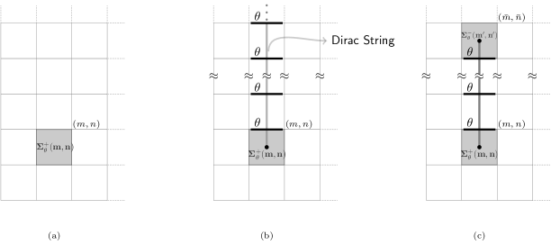
Figure 12: The disorder operator $\Sigma_{\theta}^{+}(m,n)$ creating a magnetic vortex at $(m,n)$ (a) in the dual spin description, (b) in the original Kogut-Susskind gauge description but now with an infinitely long Dirac string, (c) a vortex-anti-vortex pair connected through a finite length Dirac string. The dark heavy horizontal links across the Dirac strings in (b) and (c) represent rotations of the Kogut-Susskind link operators $U(m-1,n^{\prime};\hat{1}),n^{\prime}\geq n$ by $\theta$. More details are given in Appendix B.2.

The Hamiltonian of pure SU(N) gauge theory in terms of the dual operators is

$$H=\sum_{m,n\in\Lambda}\frac{g^{2}}{2}\Bigg{\{}\Big{[}\vec{\cal E}_{-}(m+1,n+1)+\vec{\cal E}_{+}(m+1,n)+{\Delta}_{XY}(m,n)\Big{]}^{2}$$

$$+\Big{[}\vec{\cal E}_{+}(m+1,n+1)+R_{bc}({W}(m,n))\vec{\cal E}_{-}^{c}(m,n+1)+\Delta_{Y}(m,n)\Big{]}^{2}\Bigg{\}}$$

$$~{}~{}+\frac{1}{2g^{2}}\Big{(}2N-(Tr~{}{\cal W}(m,n)+h.c)\Big{)}\equiv g^{2}\tilde{H}_{E}+\frac{1}{g^{2}}\tilde{H}_{B}.$$ (62)

In (62) we have defined msprd , ${\Delta}^{a}_{XY}(m,n)\equiv\delta_{m,0}\sum\limits_{\bar{m}=m+2}^{\sf N}\sum\limits_{\bar{n}=1}^{\sf N}{\mathbb{L}}^{a}(\bar{m},\bar{n})$ and ${\Delta}^{a}_{Y}(m,n)\equiv\sum\limits_{\bar{n}=n+2}^{\sf N}{\mathbb{L}}^{a}(m,\bar{n})$, where ${\mathbb{L}}(m,n)$ is given in the equation (59).

Thus the SU(N) Kogut-Susskind Hamiltonian in its dual description (unlike the $Z_{2}$ lattice gauge theory Ising model Hamiltonian) becomes non-local. The non-localities in (62) comes from the terms ${\cal R}({\cal W}),{\Delta}^{a}_{XY}(m,n)$ and ${\Delta}^{a}_{Y}(m,n)$. But, since ${\cal R}({\cal W})=1+o(g)+o(g^{2})+\cdots$ , ${\mathbb{L}}$ is of order $g^{n},~{}(n\geq 1)$ which implies that ${\Delta}^{a}_{XY}(m,n)$ and ${\Delta}^{a}_{Y}(m,n)$ are both at least of the order of $g$. Therefore we expect that in the $g^{2}\rightarrow 0$ continuum limit, these non-local parts can be ignored to the lowest order at low energies. This leads to a simplified local effective Hamiltonian $H_{spin}$ which may describe pure SU(N) gauge theory at low energies, sufficiently well.

$$H_{spin}=\frac{g^{2}}{2}\left\{\sum\limits_{p=1}^{\cal P}4\vec{\cal E}^{~{}2}(p)+\sum_{<p,p^{\prime}>}\vec{\cal E}_{-}(p)\cdot\vec{\cal E}_{+}(p^{\prime})\right\}+$$

$$\frac{1}{2g^{2}}\Bigg{\{}2N-\left(Tr{\cal W}(p)+h.c\right)\Bigg{\}}\equiv\frac{g^{2}}{2}{\tilde{H}}^{\prime}_{E}+\frac{1}{2g^{2}}{\tilde{H}}_{B}.~{}~{}$$ (63)

In (63), ${<p,p^{\prime}>}$ is used to show the nearest plaquettes. The above simplified SU(N) spin Hamiltonian $H_{spin}$ describes nearest neighbouring SU(N) spins interacting through their left and right electric fields. All interactions are now contained in the ’electric part’ $\tilde{H}^{\prime}_{E}$ and the magnetic part $\tilde{H}_{B}\sim Tr{\cal W}(p)$ is a non-interacting term. As a result, the coupling constant of the dual model is the inverse of that of the original Kogut Susskind model:

$H^{SU(N)}_{gauge}\big{(}\frac{1}{g^{2}}\big{)}\simeq H^{SU(N)}_{spin}\big{(}{g^{2}}\big{)}$.

We have used $\simeq$ above to state that this equivalence is only within the physical Hilbert space ${\cal H}^{p}$. The above relation is SU(N) analogue of the $Z_{2}$ result $H^{{}^{Z_{2}}}_{gauge}(\lambda)\simeq H^{{}^{Z_{2}}}_{spin}(\lambda^{-1})$ discussed earlier.

Note that the global SU(N) invariance (58) of the dual SU(N) spin model is to be fixed by imposing the Gauss law (59) at the origin. The degrees of freedom before and after duality match exactly as follows. We have converted the initial $3{\cal L}$ Kogut-Susskind link operators into $3{\cal P}$ plaquette spin operators and $3({\cal N}-1)$ string operators (see Table 1) and ${\cal L}={\cal P}+({\cal N}-1)$. There are ${\cal N}$ mutually independent Gauss laws in SU(N) (but $({\cal N}-1)$ in $Z_{2}$ case) lattice gauge theory. Out of these, $({\cal N}-1)$ freeze the $({\cal N}-1)$ strings. We are thus left with a single Gauss law constraint (59) in SU(N) spin model after duality and none in $Z_{2}$ case.

II.3.6 SU(N) Magnetic disorder operator

Exploiting duality transformations, we now construct a SU(N) gauge invariant operator which measure the magnetic disorder in the gauge system hooft . Such disorder operators and their correlations in the context of 2-dimensional Ising model and Kramers-Wannier duality have been extensively discussed in the path integral approach by Kadanoff and Ceva kadanoff . These disorder variables were called magnetic dislocations.

In this section we work with dual SU(2) spin model with global SU(2) gauge invariance (58). We construct a SU(2) invariant magnetic disorder or vortex operator which creates a magnetic vortex on a single plaquette. We focus on a single plaquette $p=(m,n)$ in $\Lambda$ with fixed $m$ and $n$ as in Figure (12) and write the SU(2) magnetic spin operator ${\cal W}_{\alpha\beta}$ in the magnetic field eigen basis as:

$${\cal W}{(m,n)}\equiv cos\left(\frac{\omega_{(m,n)}}{2}\right)\sigma_{0}+i\left(\hat{w}_{(m,n)}\cdot\vec{\sigma}\right)\sin\left(\frac{\omega_{(m,n)}}{2}\right)$$

$$\hskip 51.21504pt\hat{w}_{(m,n)}\cdot\hat{w}_{(m,n)}=1.$$ (64)

In (64), $\omega(m,n)$ are gauge invariant angles, $\hat{w}(m,n)$ are the unit vectors in the group manifold $S^{3}$ and $\sigma_{0},\vec{\sigma}$ are the unit, Pauli matrices. Under global gauge transformation $\Lambda\equiv\Lambda(0,0)$ in (58), $(\omega,\hat{w})$ transform as:

$$\omega(m,n)\rightarrow\omega(m,n),~{}~{}\hat{w}^{a}(m,n)\rightarrow R_{ab}(\Lambda)~{}\hat{w}^{b}(m,n).$$ (65)

Above, $R_{ab}(\Lambda)$ are given in (46). We define two unitary operators:

$${\Sigma}^{\pm}_{\theta}(m,n)\equiv exp~{}i\Big{(}{\hat{w}}(m,n)\cdot{\cal E}_{\pm}(m,n)\phantom{.}{\theta}\Big{)},$$ (66)

which are located on a plaquette $p\equiv(m,n)$ as shown in the Figure 12-a. They both are gauge invariant because ${\cal E}_{\pm}^{a}(m,n)$ and $\hat{w}(m,n)$ gauge transform like vectors. In other words, $\left[{\cal G}^{a},\Sigma^{\pm}_{\theta}(m,n)\right]=0$, where ${\cal G}^{a}$ is defined in (59). As the left and right SU(N) electric scalar potentials are related through (54), ${\Sigma}^{\pm}_{\theta}(m,n)$ are not independent and satisfy:

$${\Sigma}^{+}_{\theta}(m,n)~{}{\Sigma}^{-}_{\theta}(m,n)={\Sigma}^{-}_{\theta}(m,n)~{}{\Sigma}^{+}_{\theta}(m,n)={\it I}.$$ (67)

Above ${\it I}$ denotes the unit operator in the physical Hilbert space ${\cal H}^{p}$ and $\Sigma_{\theta}^{-}=\Sigma_{-\theta}^{+}$. The physical meaning of the operators $\Sigma_{\theta}^{\pm}(m,n)$ is simple and exactly similar in spirit as $\Sigma_{\pi}(m,n)$ in (43) in the $Z_{2}$ lattice gauge theory case. The non-abelian electric scalar potentials ${\cal E}^{a}_{\pm}(m,n)$ are conjugate to the magnetic flux operators ${\cal W}_{\alpha\beta}(m,n)$. They satisfy the canonical commutation relations (53a). Therefore the gauge invariant operator ${\Sigma}^{\pm}_{\theta}(m,n)$ locally and continuously changes the magnetic flux on the plaquette $p=(m,n)$ as a function of $\theta$ . They are the magnetic vortex operators. To see this explicitly, we consider eigenstates $\ket{\omega(m,n),\hat{w}(m,n)}$ of ${\cal W}_{\alpha\beta}(m,n)$ on a single plaquette. These states are explicitly constructed in (104) in Appendix C. They satisfy:

$$Tr{\cal W}~{}\ket{\omega,\hat{w}}=2\cos\left(\frac{\omega}{2}\right)~{}\ket{\omega,\hat{w}}.$$ (68)

We have ignored the irrelevant plaquette index $p\equiv(m,n)$ in (68) as we are dealing with a single plaquette. It is easy to check:

$$\ket{\omega,\hat{w}}_{\pm\theta}\equiv\Sigma_{\theta}^{\pm}\ket{\omega,\hat{w}}=\ket{\omega\pm\theta,\hat{w}},$$ (69)

implying,

$$Tr~{}{\cal W}~{}|\omega,\hat{w}\rangle_{\pm\theta}=2~{}cos\left(\frac{\omega\pm\theta}{2}\right)~{}|\omega,\hat{w}\rangle_{\pm\theta}.$$ (70)

The equations (68) and (70) state:

$$\Sigma^{\pm}_{2\pi}\phantom{}\left(Tr{\cal W}\right)=-~{}\left(Tr{\cal W}\right)\phantom{.}\Sigma^{\pm}_{2\pi}.$$ (71)

We thus recover the standard Wilson-’t Hooft loop $Z_{2}$ algebra hooft ; to for SU(2) at $\theta=2\pi$. Similarly, we get

$$\left(Tr{\cal W}^{q}\right)~{}\Sigma^{\pm}_{2\pi}=\left(-1\right)^{q}~{}\Sigma^{\pm}_{2\pi}~{}\left(Tr{\cal W}^{q}\right).$$ (72)

These relations are analogous to the $Z_{2}$ results (44). The operator $\Sigma_{2\pi}$ is the well known SU(2) ’t Hooft operator. The relations (71) and (72) can be easily generalized to an arbitrary Wilson loop $W_{C}$. In the dual spin model any Wilson loop can be written in terms of the ${\cal P}$ fundamental loops ${\cal W}_{\alpha\beta}$ as shown in Figure 13:

$$W_{C}={\cal W}(p_{1})~{}{\cal W}(p_{2})~{}{\cal W}(p_{3})\cdots\cdots{\cal W}(p_{n_{c}}).$$ (73)

Here $p_{1}$ is the plaquette operator in the bottom right corner of $C$ and $p_{n_{c}}$ is the plaquette operator at the left top corner of $C$. Now the factor $(-1)^{q}$ in (72) is the phase when the curve $C$ winds the magnetic vortex at $(m,n)$ (created by $\Sigma^{\pm}_{2\pi}(m,n)$) $q$ number of times.

The plaquette magnetic flux or the vortex operators $\Sigma^{\pm}_{\theta}(m,n)$ in (66) can also be written as a non-local sum of Kogut-Susskind link electric fields along a line and the corresponding parallel transports using (51b). The magnetic charge on the plaquette $p=(m,n)$ thus develops an infinite Dirac string in the original (standard) $\{E^{a}(l);U(l)\}$ description. This is similar to the discrete $Z_{2}$ disorder operator ${\Sigma}(m,n)$ written in terms of the original electric field operators $\sigma_{1}(m,n^{\prime})$ in (41) and (43). The Dirac string is shown in Figure 12-b for our choice of canonical transformations. Note that it can be rotated by choosing a different scheme for the canonical transformations. Only the end points of Dirac strings (location of the vortex) are physical and independent of the canonical transformation schemes. This is exactly analogous to the rotations of the $Z_{2}$ Dirac strings and the location of $Z_{2}$ vortices in (41) or (43). Their orientations do not matter as Dirac strings themselves are invisible. In $Z_{2}$ or U(1) gauge theories they are trivially invisible as two horizontal links in Figure (12)-b change by opposite phases which commute through the plaquette links and cancel each other. However, in the present non-abelian case, the non-local parallel transport $R_{ab}(S(m,n;n^{\prime}))$ in relation (51b) plays an important role in making the Dirac string invisible. These issues are further discussed in detail in Appendix B.2. We note that the disorder operators in the strong coupling vacuum satisfy:

$$\left\langle 0|\Sigma^{\pm}_{\theta}(m,n)|0\right\rangle=1.$$

The vacuum expectation values of all Wilson loops, on the other hand, are zero: $\left\langle 0|W_{C}(U)|0\right\rangle=0$. It will be interesting to study the behavior of the vacuum expectation values of $\Sigma_{\theta}^{\pm}$ for the finite values of the coupling along with the vacuum correlation functions $\left\langle\Sigma^{\pm}_{\theta}(p)\Sigma^{\mp}_{\theta}(p^{\prime})\right\rangle$, shown in Figure 12-c, as $|p-p^{\prime}|\rightarrow\infty$. The work in this direction is in progress and will be reported elsewhere.

III A variational ground state of SU(N) spin model

In this section, we study the ground state of the dual spin model with nearest neighbor interactions. We then compare the results with those obtained from the variational analysis of the standard Kogut Susskind formulation arisue ; suranyi ; drstump . Note that after canonical transformations each plaquette loop is a fundamental degree of freedom. Therefore gauge invariant computations in the dual spin model become much simpler. For simplicity we consider $N=2$. For the ground state of SU(2) gauge theory, the magnetic fluctuations in a region are independent of fluctuation in another region sufficiently far away feynman ; greensite . So, the largest contributions to the vacuum state comes from states with little magnetic correlations. Therefore we use the following separable state without any spin-spin correlations as our variational ansatz:

$$|\psi_{0}\rangle =e^{S/2}|0\rangle; S =\alpha\sum\limits_{{p}}Tr{\cal W}({p}).$$

$$=\prod\limits_{p}~{}|\psi_{0}\rangle_{p}.$$ (74)

Above, $|0\rangle$ is the strong coupling vacuum state defined by ${\cal E}^{a}_{\pm}(m,n)|0\rangle=0$ and $\alpha$ is the variational parameter. Since this state doesn’t have long distance correlations, it satisfies Wilson’s area law criterion. We consider a Wilson loop $Tr~{}(W_{C})$ along a large space loop C on the lattice and compute its ground state expectation value: $<\psi_{0}|TrW_{C}|\psi_{0}>/~{}\langle\psi_{0}|\psi_{0}\rangle$.

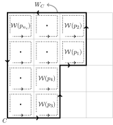
Figure 13: A Wilson loop $W_{C}$ can be written as the product of fundamental plaquette loop operators ${\cal W}(p)$. $W_{C}={\cal W}(p_{1})~{}{\cal W}(p_{2})~{}{\cal W}(p_{3})\cdots\cdots{\cal W}(p_{n_{c}})$. The tails of the fundamental plaquette loop operators connecting them to the origin (see Figure 10-a) are not shown for clarity.

As shown in the Appendix C (see (107)):

$$\frac{\langle\psi_{0}|TrW_{C}|\psi_{0}\rangle}{\langle\psi_{0}|\psi_{0}\rangle} =2\left(\frac{I_{2}(2\alpha)}{I_{1}(2\alpha)}\right)^{n_{c}}=2e^{-n_{c}\ln\left(\frac{I_{1}(2\alpha)}{I_{2}(2\alpha)}\right)}$$ (75)

In (75), we have used the decomposition (73) and $n_{c}$ is the number of plaquettes in the loop C. The function $I_{l}$ is the $l$-th order modified Bessel function of the first kind. The string tension is given by $\sigma_{T}(\alpha)=\ln\left(\frac{I_{1}(2\alpha)}{I_{2}(2\alpha)}\right)$.

We now calculate $\alpha$ by minimizing

$$\langle H_{spin}\rangle=\frac{\langle\psi_{0}|H_{spin}|\psi_{0}\rangle}{\langle\psi_{0}|\psi_{0}\rangle}.$$

In order to calculate $\langle H_{spin}\rangle$, we first find the expectation value of ${\cal E}_{-}(p)\cdot{\cal E}_{+}(p^{\prime})$ and ${\cal E}(p)\cdot{\cal E}(p)\equiv{\cal E}_{+}(p)\cdot{\cal E}_{+}(p)\equiv{\cal E}_{-}(p)\cdot{\cal E}_{-}(p)$ in (63). This calculation is done in Appendix D. The expectation values are (see (115))

$$\langle{\cal E}_{-}(p)\cdot{\cal E}_{+}(p^{\prime})\rangle=0,~{}~{}~{}~{}\langle{\cal E}(p)\cdot{\cal E}(p)\rangle=\frac{3\alpha}{16}\langle Tr{\cal W}(p)\rangle.$$

Putting $n_{c}=1$ in equation (75), we get $\langle Tr{\cal W}(p)\rangle=\frac{2I_{2}(2\alpha)}{I_{1}(2\alpha)}$. Therefore the expectation value of the effective Hamiltonian $H_{spin}$ is

$$\frac{\langle\psi_{0}|H_{spin}|\psi_{0}\rangle}{\langle\psi_{0}|\psi_{0}\rangle} =2{\cal P}\left\{\left(\frac{3\alpha}{4}g^{2}-\frac{1}{g^{2}}\right)\frac{I_{2}(2\alpha)}{I_{1}(2\alpha)}+\frac{1}{g^{2}}\right\}.$$ (76)

Above, ${\cal P}$ is the number of plaquettes in the lattice. $\frac{I_{2}(2\alpha)}{I_{1}(2\alpha)}$ is a monotonously increasing bounded function of $\alpha$. It takes values between $+1$ and $-1$ with $+1$ at $\alpha\rightarrow\infty$ and $-1$ at $\alpha\rightarrow-\infty$. In the weak coupling limit, $g^{2}\rightarrow 0$, $\frac{I_{2}(2\alpha)}{I_{1}(2\alpha)}$ should be maximum for the expectation value of $H_{spin}$ to be minimum and therefore, $\alpha\rightarrow\infty$. But, using the asymptotic form of the modified Bessel function of the first kind $I_{l}(2\alpha)$,

$$I_{l}(2\alpha)\xrightarrow{\alpha\rightarrow\infty}\frac{e^{2\alpha}}{\sqrt{2\pi(2\alpha)}}\left(1+\frac{(1-2l)(1+2l)}{16\alpha}+\cdots\right)$$

In the weak coupling limit , $\frac{I_{2}(2\alpha)}{I_{1}(2\alpha)}\approx 1-\frac{3}{4\alpha}$. Hence,

$$\frac{\langle\psi_{0}|H_{spin}|\psi_{0}\rangle}{\langle\psi_{0}|\psi_{0}\rangle} =\sum\limits_{p}2\left\{\left(\frac{3\alpha}{4}g^{2}-\frac{1}{g^{2}}\right)\left(1-\frac{3}{4\alpha}\right)+\frac{1}{g^{2}}\right\}$$ (77)

Minimizing the expectation value in the weak coupling limit, $\alpha=\frac{1}{g^{2}}$. The string tension is given by $\sigma_{T}(\frac{1}{g^{2}})=ln\left(I_{1}(\frac{1}{g^{2}})/I_{2}(\frac{1}{g^{2}})\right)$. This is exactly the result obtained in suranyi ; arisue using variational calculation with the fully disordered ground state and Kogut-Susskind Hamiltonian (49) which is dual to the full non-local spin Hamiltonian. As shown in Appendix D, the expectation value of the non-local part of the Hamiltonian in the variational ground state $|\psi_{0}\rangle$ vanishes. So, the simplified Hamiltonian with nearest neighbor interactions gives the same variational ground state to the lowest order as the full Hamiltonian. The disorder operator expectation value in this variational ground state is

$$\frac{\langle\psi_{0}|\Sigma_{\theta=2\pi}^{\pm}(m,n)|\psi_{0}\rangle}{\langle\psi_{0}|\psi_{0}\rangle}=\frac{16\pi^{2}}{{}_{p}\langle\psi_{0}|\psi_{0}\rangle_{{}_{p}}}=\frac{\pi\alpha}{2I_{1}(2\alpha)}.$$ (78)

Above, we have defined $p\equiv(m,n)$ and written the separable state $|\psi_{0}\rangle$ as the direct product of the state vectors corresponding to each plaquette i.e, $|\psi_{0}\rangle=\prod_{p}~{}|\psi_{0}\rangle_{p}$.

IV Summary and Discussion

In this work, we have shown that the canonical transformations provide a method to generalize Wegner duality between $Z_{2}$ lattice gauge theory and quantum Ising model to SU(N) lattice gauge theories. The similarities between $Z_{2}$ Wegner and SU(N) dualities were emphasized. The SU(N) dual formulation leads to a new gauge invariant disorder operator creating, annihilating magnetic vortices. This disorder operator can be measured in Monte-Carlo simulations. At $\theta=2\pi$ it reduces to ’t Hooft disorder operator creating center vortices. It will be interesting to see its behavior across the deconfinement transition. In the weak coupling continuum limit, the Hamiltonian of the dual model reduces to an effective SU(N) spin Hamiltonian with nearest neighbouring interactions. We use a variational analysis of the spin model with a completely disordered ground state ansatz. The effective spin Hamiltonian leads to the same results as the standard Kogut Susskind Hamiltonian. Further analysis of the SU(N) spin model and its spectrum is required. This is the subject of our future investigations. It will also be interesting to generalize these transformations to $(3+1)$ dimensions to define dual electric vector potentials with a dual gauge group. The work in this direction is also in progress.

Appendix A Wegner gauge-spin duality through canonical transformations

In this Appendix, we describe the canonical transformation involved in the construction of the duality relation between the basic operators of $Z_{2}$ gauge theory and Ising model in $2+1$ dimensions. The net effect of the canonical transformation involved in the construction of the spin operators on a single plaquette, described in section 2, can be summarized as follows:

• It replaces the top link $l_{3}$ on the plaquette by a plaquette spin operator with the same ‘electric field’ as the top link:

  $$\mu_{1}(p) =\sigma_{3}(l_{1})\sigma_{3}(l_{2})\sigma_{3}(l_{3})\sigma_{3}(l_{4}), \mu_{3}(p) =\sigma_{1}(l_{3}).$$ (79)

• The ‘electric field’ of the top link $l_{3}$ that vanishes gets absorbed into the electric fields of other links $l_{1},l_{2},l_{4}$:

  $$\bar{\sigma}_{3}(l_{1}) =\sigma_{3}(l_{1}), \bar{\sigma}_{1}(l_{1}) =\sigma_{1}(l_{1})\sigma_{1}(l_{3})$$

  $$\bar{\sigma}_{3}(l_{2}) =\sigma_{3}(l_{2}), \bar{\sigma}_{1}(l_{2}) =\sigma_{1}(l_{2})\sigma_{1}(l_{3})$$

  $$\bar{\sigma}_{3}(l_{4}) =\sigma_{3}(l_{4}), \bar{\sigma}_{1}(l_{4}) =\sigma_{1}(l_{4})\sigma_{1}(l_{3})$$ (80)

  It is convenient to call the above net canonical transformation a ‘plaquette canonical transformation (C.T)’. We now generalize the duality transformation relation to a finite lattice by iterating the plaquette C.T all over the two dimensional lattice starting from the top left plaquette of the lattice and systematically repeating it from top to bottom and left to right. We will illustrate this procedure on a $2\times 2$ lattice which contains all the essential features of the construction on any finite lattice. The sites of the lattice are labelled as $O\equiv(0,0),A\equiv(0,1),B\equiv(0,2),C\equiv(1,0),D\equiv(1,1),E\equiv(1,2),F\equiv(2,0),G\equiv(2,1),H\equiv(2,2)$ and the plaquettes are numbered from top to bottom and left to right (see Figure 14) for convenience. The dual spin operators are constructed on a $2\times 2$ lattice in 4 steps.

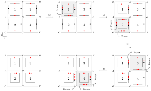
Figure 14: The ‘plaquette’ canonical transformations involved in the construction of the duality transformation between $Z_{2}$ lattice gauge theory and $Z_{2}$ spin model on a $2\times 2$ lattice. The steps (a), (b), (c) and (d) are plaquette canonical transformations on the plaquettes 1, 2, 3 and 4 respectively. The electric field $\sigma_{1}(l)$ corresponding to the vertical and horizontal links are denoted by $\bullet$ and $\blacklozenge$ respectively.

1. We begin by performing the plaquette canonical transformation (79),(80) on plaquette 1. The spin conjugate operators $\{\mu_{1}(1);\mu_{3}(1)\}$ on plaquette 1 are

   $$\mu_{1}(1)\equiv\mu_{1}(E)=\sigma_{3}(A;\hat{1})\sigma_{3}(D;\hat{2})\sigma_{3}(B;\hat{1})\sigma_{3}(A;\hat{2}),$$

   $$~{}~{}~{}~{}~{}~{}~{}~{}~{}~{}~{}~{}~{}~{}~{}~{}\mu_{3}(1)\equiv\mu_{3}(E)=\sigma_{1}(B;\hat{1}).$$ (81)

   The redefined link and string operators around plaquette 1 are

   $$\sigma_{3[x]}(D;\hat{2})=\sigma_{3}(D;\hat{2}),~{}~{}~{}\sigma_{1[x]}(D;\hat{2})=\sigma_{1}(D;\hat{2})\sigma_{1}(B;\hat{1})$$

   $$\sigma_{3[x]}(A;\hat{2})=\sigma_{3}(A;\hat{2}),~{}~{}~{}\sigma_{1[x]}(A;\hat{2})=\sigma_{1}(A;\hat{2})\sigma_{1}(B;\hat{1})$$

   $$\sigma_{3[x]}(A;\hat{1})=\sigma_{3}(A;\hat{1}),~{}~{}~{}\sigma_{1[x]}(A;\hat{1})=\sigma_{1}(A;\hat{1})\sigma_{1}(B;\hat{1}).$$

   Our notation is such that $\sigma_{3}(A;\hat{1})$ denotes the $\sigma_{3}$ variable of the link which starts at site A and is in the $\hat{1}$ direction. The subscript $[x]$ on $\sigma_{3[x]}(A;\hat{1})$ indicates that the electric field $\sigma_{1}(A;\hat{1})$ absorbs the electric field of the vanishing horizontal link $(B;\hat{1})$ to become $\sigma_{1[x]}(A;\hat{1})$ during the plaquette C.T. Note that by our convention, the plaquette or spin operators are labelled by the top right corner of the plaquette. This plaquette C.T is illustrated in Figure 14 (a). As a result of Gauss law at B:

   $$\sigma_{1[x]}(A;\hat{2})\equiv{\cal G}(B)\approx 1.$$

   Therefore, $\left\{\sigma_{1[x]}(A;\hat{2});\sigma_{3[x]}(A;\hat{2})\right\}\equiv\left\{\bar{\sigma}_{1}(B);\bar{\sigma}_{3}(B)\right\}$ are frozen and hence decouple from the physical Hilbert space. Again, as in the main text, the string operators are labelled by their right/top endpoints. We are now left with the conjugate spin operators $\left\{\mu_{1}(1);\mu_{3}(1)\right\}$ and the two link conjugate pair operators $\left\{\sigma_{1[x]}(D;\hat{2});\sigma_{3[x]}(D;\hat{2})\right\},\left\{\sigma_{1[x]}(A;\hat{1});\sigma_{3[x]}(A;\hat{1})\right\}$. These link operators undergo further canonical transformations.

2. We now iterate the plaquette C.T. on plaquette 2 to construct the spin or plaquette conjugate operators $\left\{\mu_{1}(2);\mu_{3}(2)\right\}$ and the link conjugate operators $\left\{\sigma_{1[x]}(C;\hat{2});\sigma_{3[x]}(C;\hat{2})\right\}$, $\left\{\sigma_{1[x]}(O;\hat{1});\sigma_{3[x]}(O;\hat{1})\right\}$, $\left\{\sigma_{1[x]}(O;\hat{2});\sigma_{3[x]}(O;\hat{2})\right\}$ as illustrated in Figure 14-b. The spin operators are

   $$\mu_{1}(2)\equiv\mu_{1}(D)=\sigma_{3}(A;\hat{1})\sigma_{3}(O;\hat{2})\sigma_{3}(O;\hat{1})\sigma_{3}(C;\hat{2}),$$

   $$\mu_{3}(2)\equiv\mu_{3}(D)=\sigma_{1[x]}(A;\hat{1})=\sigma_{1}(A;\hat{1})\sigma_{1}(B;\hat{1})$$ (82)

   The redefined link and new string operators around plaquette 2 are

   $$\sigma_{3[x]}(C;\hat{2})=\sigma_{3}(C;\hat{2}),$$

   $$\sigma_{1[x]}(C;\hat{2})=\sigma_{1}(C;\hat{2})\sigma_{1[x]}(A;\hat{1})=\sigma_{1}(C;\hat{2})\sigma_{1}(A;\hat{1})\sigma_{1}(B;\hat{1})$$

   $$\sigma_{3[x]}(O;\hat{1})=\sigma_{3}(O;\hat{1}),$$

   $$\sigma_{1[x]}(O;\hat{1})=\sigma_{1}(O;\hat{1})\sigma_{1[x]}(A;\hat{1})={\cal G}(O){\cal G}(A){\cal G}(B)\approx 1$$

   $$\sigma_{3[x]}(O;\hat{2})=\sigma_{3}(O;\hat{2}),$$ (83)

   $$\sigma_{1[x]}(O;\hat{2})=\sigma_{1}(O;\hat{2})\sigma_{1[x]}(A;\hat{1})={\cal G}(A){\cal G}(B)\approx 1.$$

   Thus the string conjugate pairs $\left\{\sigma_{1[x]}(O;\hat{1});\sigma_{3[x]}(O;\hat{1})\right\}\equiv\left\{\bar{\sigma}_{1}(C);\bar{\sigma}_{3}(C)\right\}$ and $\left\{\sigma_{1[x]}(O;\hat{2});\sigma_{3[x]}(O;\hat{2})\right\}\equiv\left\{\bar{\sigma}_{1}(A);\bar{\sigma}_{3}(A)\right\}$ are frozen due to Gauss law at O, A and B.

3. The third step involves iterating the plaquette C.T. on plaquette 3 as shown in Figure 14(c). This leads to decoupling of $\left\{\sigma_{1[x]}(G;\hat{2});\sigma_{3[x]}(G;\hat{2})\right\}\equiv\left\{\bar{\sigma}_{1}(H);\bar{\sigma}_{3}(H)\right\}$, $\left\{\sigma_{1[xx]}(D,\hat{2});\sigma_{3[xx]}(D,\hat{2})\right\}\equiv\left\{\bar{\sigma}_{1}(E);\bar{\sigma}_{3}(E)\right\}$ due to the $Z_{2}$ Gauss laws at E and H. The canonical transformations on plaquette 3 defining the spins are

   $$\mu_{1}(3)\equiv\mu_{1}(H)=\sigma_{3}(E;\hat{1})\sigma_{3}(G;\hat{2})\sigma_{3}(D;\hat{1})\sigma_{3}(D;\hat{2}),$$

   $$\mu_{3}(3)\equiv\mu_{3}(H)=\sigma_{3}(E;\hat{1}).$$ (84)

   The redefined links and strings around plaquette 3 are

   $$\sigma_{3[xx]}(D,\hat{2})=\sigma_{3[x]}(D;\hat{2})=\sigma_{3}(D;\hat{2}),$$

   $$\sigma_{1[xx]}(D;\hat{2})=\sigma_{1[x]}(D;\hat{2})\sigma_{1}(E;\hat{1})={\cal G}(E)\approx 1$$

   $$\sigma_{3[x]}(G;\hat{2})=\sigma_{3}(G;\hat{2}),$$

   $$\sigma_{1[x]}(G;\hat{2})=\sigma_{1}(G;\hat{2})\sigma_{1}(E;\hat{1})={\cal G}(H)\approx 1$$

   $$\sigma_{3[x]}(D;\hat{1})=\sigma_{3}(D;\hat{1}),$$

   $$\sigma_{1[x]}(D;\hat{1})=\sigma_{1}(D;\hat{1})\sigma_{1}(E;\hat{1})$$ (85)

4. Finally, we iterate the plaquette C.T. on plaquette 4 which are shown in Figure 14(d). The conjugate spin operators $\{\mu_{1}(4);\mu_{3}(4)\}$ on plaquette 4 are

   $$\mu_{1}(4)\equiv\mu_{1}(G)=\sigma_{3}(D;\hat{1})\sigma_{3}(F;\hat{2})\sigma_{3}(C;\hat{1})\sigma_{3}(C;\hat{2}),$$

   $$\mu_{3}(4)\equiv\mu_{3}(G)=\sigma_{1[x]}(D;\hat{1})=\sigma_{1}(D;\hat{1})\sigma_{1}(E;\hat{1})$$ (86)

   The remaining string operators are

   $$\sigma_{3[xx]}(C;\hat{2})=\sigma_{3[x]}(C;\hat{2})=\sigma_{3}(C;\hat{2}),$$

   $$\sigma_{1[xx]}(C;\hat{2})=\sigma_{1[x]}(C;\hat{2})\sigma_{1[x]}(D;\hat{1})={\cal G}(D){\cal G}(E)\approx 1$$

   $$\sigma_{3[x]}(C;\hat{1})=\sigma_{3}(C;\hat{1})$$

   $$\sigma_{1[x]}(C;\hat{1})=\sigma_{1}(C;\hat{1})\sigma_{1[x]}(D;\hat{1})$$

   $$\hskip 42.67912pt={\cal G}(C){\cal G}(O){\cal G}(A){\cal G}(D){\cal G}(B){\cal G}(E)\approx 1$$

   $$\sigma_{3[x]}(F;\hat{2})=\sigma_{3}(F;\hat{2}),$$ (87)

   $$\sigma_{1[x]}(F;\hat{2})=\sigma_{1}(F;\hat{2})\sigma_{1[x]}(D;\hat{1})={\cal G}(G){\cal G}(H)\approx 1.$$

   Gauss laws at $O,A,B,C,D,E,G$ and H implies that the remaining string operators $\left\{\sigma_{1[xx]}(C;\hat{2});\sigma_{3[xx]}(C;\hat{2})\right\}\equiv\left\{\bar{\sigma}_{1}(D);\bar{\sigma}_{3}(D)\right\}$, $\left\{\sigma_{1[x]}(C,\hat{1});\sigma_{3[x]}(C,\hat{1})\right\}\equiv\left\{\bar{\sigma}_{1}(F);\bar{\sigma}_{3}(F)\right\}$ and $\left\{\sigma_{1[x]}(F,\hat{2});\sigma_{3[x]}(F,\hat{2})\right\}\equiv\left\{\bar{\sigma}_{1}(G);\bar{\sigma}_{3}(G)\right\}$ are frozen. As a result, after the series of 4 plaquette C.T.s, all the Gauss law constraints are solved. Only the plaquette/spin variables $\left\{\mu_{1}(1);\mu_{3}(1)\right\},\left\{\mu_{1}(2);\mu_{3}(2)\right\},\left\{\mu_{1}(3);\mu_{3}(3)\right\}$ and $\left\{\mu_{1}(4);\mu_{3}(4)\right\}$ remains in the physical Hilbert space. This leads to a dual $Z_{2}$ spin model. These results can be directly generalized to any finite lattice without any new issues, to give the duality relations (28a),(28b), (30a)-(30b).

Appendix B Non-abelian Duality & Non-locality

In this Appendix we discuss the role of non local terms in non-abelian duality transformations. We show that they lead to magical cancellations required for (a) the SU(N) Gauss laws to be satisfied, (b) the Dirac strings associated with U(1) vortices to be invisible. These non-trivial cancellations should be contrasted with the similar but trivial $Z_{2}$ lattice gauge theory cancellations in terms of the electric scalar potentials discussed in section II.2.4 and illustrated in Figure 7.

B.1 SU(N) Gauss laws & Solutions

In this part we show that the dual SU(N) electric scalar potentials solve the local SU(N) Gauss laws at all lattice sites except the origin. At the origin they lead to the global constraints (59). This is SU(N) generalization of the $Z_{2}$ results discussed in section II.2.4.

We show explicit calculations for all the possible cases namely ($m\neq 0,n\neq 0$), ($m=0,n\neq 0$), ($m\neq 0,n=0$) and ($m=0,n=0$).

• $m\neq 0,n\neq 0$

  The Kogut-Susskind SU(N) electric fields meeting at $(m,n)$ in terms of the spin operators (61) are:

  $$E_{+}^{a}(m,n;\hat{1})=\underbrace{R_{ab}({\sf T}^{\dagger}(m,n))\bigg{[}{\cal E}^{b}_{+}(m+1,n)+{\cal E}_{-}^{b}(m+1,n+1)\bigg{]}}_{T_{1}}$$

  $$E_{+}^{a}(m,n;\hat{2})=\underbrace{R_{ab}({\sf T}^{\dagger}(m,n))\bigg{[}\sum\limits_{\bar{n}=n+2}^{{{\sf N}}}\{{\cal E}_{+}^{b}(m+1,\bar{n})+{\cal E}_{-}^{b}(m+1,\bar{n})\}+{\cal E}_{+}^{b}(m+1,n+1)\bigg{]}}_{T_{2}}+\underbrace{R_{ab}(U^{\dagger}(m-1,n;\hat{1})){\sf T}^{\dagger}(m-1,n){\cal E}_{-}^{b}(m,n+1)}_{T_{3}}$$

  $$E_{-}^{a}(m,n;\hat{1})=\underbrace{-R_{ab}({U}^{\dagger}(m-1,n;\hat{1}){\sf T}^{\dagger}(m-1,n){\cal E}_{-}^{b}(m,n+1)}_{-T_{3}}+\underbrace{-R_{ab}({U}^{\dagger}(m-1,n;\hat{1}){\sf T}^{\dagger}(m-1,n)){\cal E}_{+}^{b}(m,n)}_{-T_{4}}$$

  $$E_{-}^{a}(m,n;\hat{2})=\underbrace{-R_{ab}({\sf T}^{\dagger}(m,n))\bigg{\{}{\cal E}_{+}^{b}(m+1,n)+{\cal E}_{-}^{b}(m+1,n+1)\bigg{\}}}_{-T_{1}}+$$ (88)

  $$\hskip 39.83368pt\underbrace{-R_{ab}({\sf T}^{\dagger}(m,n))\bigg{\{}{\cal E}_{+}^{b}(m+1,n+1)+\sum\limits_{\bar{n}=n+2}^{{\sf N}}\left[{\cal E}_{+}^{b}(m+1,\bar{n})+{\cal E}_{-}^{b}(m+1,\bar{n})\right]\bigg{\}}}_{-T_{2}}+\underbrace{R_{ab}(U^{\dagger}(m-1,n,\hat{1}){\sf T}^{\dagger}(m-1,n)){\cal E}_{+}^{b}(m,n)}_{T_{4}}.$$

  Therefore all $T_{1},T_{2},T_{3},T_{4}$ cancel and ${\cal G}^{a}(m\neq 0,n\neq 0)=E_{+}^{a}(m,n;\hat{1})+E_{+}^{a}(m,n;\hat{2})+E_{-}^{a}(m,n;\hat{1})+E_{-}^{a}(m,n;\hat{2})\equiv 0.$

• $m=0,~{}n\neq 0$

  Similarly, the SU(N) electric fields at $(0,n\neq 0)$ in terms of dual SU(N) spin operators in (61) are

  $$E_{+}^{a}(0,n;\hat{1})=R_{ab}({\sf T}(0,n))\big{\{}\underbrace{{\cal E}^{b}_{-}(1,n+1)}_{T_{1}}+\underbrace{{\cal E}^{b}_{+}(1,n)}_{T_{2}}\big{\}}$$

  $$E_{+}^{a}(0,n;\hat{2})=R_{ab}({\sf T}(0,n))\big{\{}\underbrace{{\cal E}^{b}_{+}(1,n+1)}_{T_{3}}+\underbrace{\sum\limits_{\bar{n}=n+2}^{\sf N}{\mathbb{L}}^{b}(1,\bar{n})}_{T_{4}}\big{\}}$$ (89)

  $$E_{-}^{a}(0,n;\hat{2})=-R_{ab}(U(0,m,\hat{2}))E_{+}^{b}(0,n-1,\hat{2})=-R_{ab}({\sf T}(0,n))\big{\{}{\cal E}^{b}_{+}(1,n)+\sum\limits_{\bar{n}=n+1}^{\sf N}{\mathbb{L}}^{b}(1,\bar{n})\big{\}}$$

  $$=-R_{ab}({\sf T}(0,n))\big{\{}{\cal E}^{b}_{+}(1,n)+{\mathbb{L}}^{b}(1,{n+1})+\sum\limits_{\bar{n}=n+2}^{\sf N}{\mathbb{L}}^{b}(1,\bar{n})\big{\}}$$

  $$=-R_{ab}({\sf T}(0,n))\big{\{}\underbrace{{\cal E}^{b}_{+}(1,n)}_{T_{2}}+\underbrace{{\cal E}^{b}_{+}(1,n+1)}_{T_{3}}+\underbrace{{\cal E}^{b}_{-}(1,n+1)}_{T_{1}}+\underbrace{\sum\limits_{\bar{n}=n+2}^{\sf N}{\mathbb{L}}^{b}(1,\bar{n})}_{T_{4}}\big{\}}.$$ (90)

  All $T_{1},T_{2},T_{3},T_{4}$ cancel and ${{\cal G}^{a}(0,n\neq 0)}=E_{+}^{a}(0,n;\hat{1})+E_{+}^{a}(0,n;\hat{2})+E_{-}^{a}(0,n;\hat{2})\equiv 0$.

• $m\neq 0,n=0$

  The Kogut-Susskind electric fields at site $(m\neq 0,0)$ are

  $$E_{+}^{a}(m,0,\hat{1})=R_{ab}({\sf T}(m,0))\Big{\{}\underbrace{{\cal E}_{-}^{b}(m+1,1)}_{T_{1}}+\underbrace{\sum\limits_{\bar{m}=m+2}^{\sf N}\sum\limits_{\bar{n}=1}^{\sf N}{\mathbb{L}}^{b}(\bar{m},\bar{n})}_{T_{2}}\Big{\}}$$

  $$E_{+}^{a}(m,0,\hat{2})=R_{ab}({\sf T}(m,0))\Big{\{}\underbrace{{\cal E}_{+}^{b}(m+1,1)}_{T_{3}}+\underbrace{{\cal E}_{-}^{b}(m,1)}_{T_{4}}+\underbrace{\sum_{\bar{n}=2}^{\sf N}{\mathbb{L}}^{b}(m+1,\bar{n})}_{T_{5}}\Big{\}}$$ (91)

  $$E_{-}^{a}(m,0,\hat{1})=R_{ab}({\sf T}(m-1,0,\hat{1}))E_{+}^{a}(m-1,0,\hat{1})=-R_{ab}({\sf T}(m,0))\Big{\{}{\cal E}_{-}^{b}(m,1)+\sum\limits_{\bar{m}=m+1}^{\sf N}\sum\limits_{\bar{n}=1}^{\sf N}{\mathbb{L}}^{b}(\bar{m},\bar{n})\Big{\}}$$

  $$=-R_{ab}({\sf T}(m,0))\Big{\{}\underbrace{{\cal E}_{-}^{b}(m,1)}_{T_{4}}+\underbrace{{\cal E}^{b}_{+}(m+1,1)}_{T_{3}}+\underbrace{{\cal E}^{b}_{-}(m+1,1)}_{T_{1}}+\underbrace{\sum\limits_{\bar{n}=2}^{\sf N}{\mathbb{L}}^{b}(m+1,\bar{n})}_{T_{5}}+\underbrace{\sum\limits_{\bar{m}=m+2}^{\sf N}\sum\limits_{\bar{n}=1}^{\sf N}{\mathbb{L}}^{b}(\bar{m},\bar{n})}_{T_{2}}\Big{\}}$$ (92)

  As before, all $T_{1},T_{2},T_{3},T_{4},T_{5}$ cancel leading to ${\cal G}^{a}(m\neq 0,n=0)=E_{+}^{a}(m,0;\hat{1})+E_{+}^{a}(m,0;\hat{2})+E_{-}^{a}(m,0;\hat{1})\equiv 0$.

• $m=0,~{}n=0$

  The electric fields $E_{+}^{a}(0,0;\hat{1})$ and $E_{+}^{a}(0,0;\hat{2})$ in (61) are

  $$\hskip 56.9055ptE_{+}^{a}(0,0;\hat{1})={\cal E}_{-}^{a}(1,1)+\sum\limits_{\bar{m}=2}^{{\sf N}}\sum\limits_{\bar{n}=1}^{{\sf N}}{\mathbb{L}}^{a}(\bar{m},\bar{n})\hskip 56.9055ptE_{+}^{a}(0,0;\hat{2})={\cal E}_{+}^{a}(1,1)+\sum\limits_{\bar{n}=2}^{{\sf N}}{\mathbb{L}}^{a}(1,\bar{n}).$$ (93)

  Therefore the Gauss law operator at the origin is given by:

  $${\cal G}^{a}(0,0)=E_{+}^{a}(0,0;\hat{1})+E_{+}^{a}(0,0;\hat{2})=\sum\limits_{\bar{m}=1}^{{\sf N}}\sum\limits_{\bar{n}=1}^{{\sf N}}{\mathbb{L}}^{a}(\bar{m},\bar{n})=0.$$ (94)

Thus the $SU(N)$ Gauss law constraints at the origin are not redundant and lead to the residual global SU(N) Gauss law (59) in terms of the SU(N) spin operators. Note that in the abelian $U(1)$ case these cancellations are trivial as there are no color indices and $R_{ab}(U)\rightarrow 1$. The global Gauss law constraint identically vanishes as ${\mathbb{L}}\equiv 0$ in the abelian case.

B.2 The invisible Dirac strings

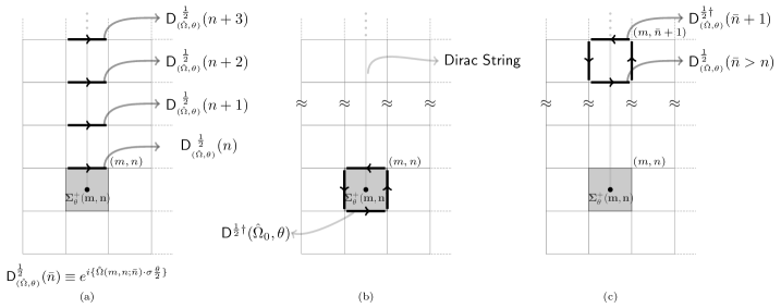
Figure 15: The invisible Dirac strings. The disorder operator $\Sigma_{\theta}^{+}(m,n)$ rotates (a) all horizontal link operators $U(m-1,\bar{n}\geq n;\hat{1})$ by a factor ${\sf D}^{\frac{1}{2}}_{\theta}(\bar{n})\equiv D^{\frac{1}{2}}(\hat{\Omega}(m,n;\bar{n}),\theta)$ in (97), (100), (b) the plaquette operator ${U}^{p}(m,n)$ rotates by ${\sf D}^{\frac{1}{2}\dagger}(\hat{\Omega}_{0},\theta)$ as in (99) (c) all other plaquette operators ${U}^{p}(m,\bar{n}>n)$ do not rotate. As shown in (102), the two factors ${\sf D}^{\frac{1}{2}\dagger}_{\theta}(\bar{n})$ and ${\sf D}^{\frac{1}{2}}({\bar{n}}+1)$ cancel highlighting the role of non-locality in non-abelian duality. The plaquette loop operators $U^{p}(\bar{m}\neq m,\bar{n})$ are trivially invariant under $\Sigma_{\theta}^{+}(m,n)$. At $\theta=2\pi$, all ${\sf D}_{(\hat{\Omega},\theta=2\pi)}^{~{}\frac{1}{2}}(n)=-1$ in (a) and all dark horizontal links change sign creating a $Z_{2}$ center vortex at $(m,n)$ hooft .

In this part we show how the SU(N) duality transformations make the non-local Dirac strings invisible. We start with the Dirac strings in the simple $Z_{2}$ lattice gauge theory. The $Z_{2}$ magnetic vortex operators (43) is

$${\Sigma}_{\pi}(m,n)=exp~{}i\Bigg{\{}\sum_{\bar{n}=n}^{\infty}E(m-1,\bar{n};\hat{1})~{}\pi\Big{\}}.$$ (95)

It is clear that this rotation operator by $\pi$ flips all

$$\sigma_{3}(m^{\prime},\bar{n};\hat{1}),~{}~{}~{}~{}m^{\prime}=m-1,~{}\bar{n}\geq n$$

along an infinitely long vertical Dirac string. The remaining operators over the entire lattice remain unaffected. Note that only the end point of the Dirac string is visible where $\Sigma_{\pi}(m,n)$ creates a magnetic vortex at $(m,n)$. We now generalize this result to SU(2) lattice gauge theory. The SU(2) disorder operator is

$$~{}~{}~{}{\Sigma}^{+}_{\theta}(m,n)\equiv exp~{}i\Bigg{\{}\left({\hat{w}}(m,n)\cdot{\cal E}_{+}(m,n)\right)\theta\Bigg{\}}$$

$$~{}=exp~{}i~{}\Bigg{\{}~{}{\tiny{\sum\limits_{\bar{n}=n}^{\infty}}}\hat{\Omega}(m,n;\bar{n})\cdot E_{-}(m,\bar{n};\hat{1})~{}\theta\Bigg{\}}.$$ (96)

In (96) we have used the defining equation (51b) for the electric scalar potentials

$${\mathcal{E}}_{+}^{a}(m,n)=\sum\limits_{\bar{n}=n}^{\sf N}R_{ab}(S(m,n;\bar{n}))~{}E_{-}^{b}(m,\bar{n};\hat{1}).$$

and

$$\hat{\Omega}^{a}(m,n;\bar{n})\equiv\hat{w}^{b}(m,n)~{}R_{ba}(S(m,n;\bar{n})).$$ (97)

From (96) it is clear that the SU(2) disorder operator $\Sigma_{\theta}^{+}(m,n)$ rotates only the following Kogut-Susskind flux operators:

$$U({\bar{m}},\bar{n};\hat{1});~{}~{}~{}~{}{\bar{m}}=m-1,~{}\bar{n}\geq n.$$ (98)

All other link operators $U(\bar{m},\bar{n},\hat{i})$ over the entire lattice remain unaffected. We now show that the disorder operator $\Sigma_{\theta}^{+}(m,n)$ rotates only ${U}_{p}(m,n)$ and leaves all other plaquette operators ${U}_{p}(\bar{m},\bar{n});~{}(\bar{m},\bar{n})\neq(m,n)$ unaffected. The non-local parallel transport operators $R_{ab}(S(m,n;\bar{n}))$ in non-abelian duality transformations play extremely crucial role in the cancellations involved.

We consider two relevant cases: (a) The plaquette $U_{p}(m,n)$,   (b) The plaquettes $U_{p}(m,\bar{n}>n)$. The action of the disorder operator on these plaquettes is graphically illustrated in Figure 15. Any plaquette $U^{p}(\bar{m},\bar{n})$ with $\bar{m}\neq m$ is not affected as none of the affected links (98) are present.

• The plaquette $U_{p}(m,n)$:

  This case is illustrated in Figure 15-b. For convenience sake, we define $U^{p}(m,n)=U(m-1,n-1;\hat{1})~{}U(m,n-1;\hat{2})~{}U^{\dagger}(m-1,n;\hat{1})~{}U^{\dagger}(m-1,n-1;\hat{2})\equiv U_{1}~{}U_{2}~{}U_{3}^{\dagger}~{}U_{4}^{\dagger}.$ From (96) it is clear that the disorder operators $\Sigma^{\pm}_{\theta}(m,n)$ act only on $U^{\dagger}(m-1,n,\hat{2})\equiv U^{\dagger}_{3}$ resulting in the rotation of the $U^{p}(m,n)$:

  $$\Sigma_{\theta}^{+}(m,n){U}^{p}_{\alpha\beta}(m,n)\Sigma_{\theta}^{-}(m,n)=\Big{(}U_{1}~{}U_{2}\Big{)}_{\alpha\gamma}\Bigg{\{}\Sigma_{\theta}^{+}(m,n)~{}\left(U^{\dagger}_{3}\right)_{\gamma\delta}~{}\Sigma_{\theta}^{-}(m,n)\Bigg{\}}\left(U_{4}\right)_{\delta\beta}=\Big{(}U_{1}~{}U_{2}\Big{)}_{\alpha\gamma}~{}\left(~{}D^{\frac{1}{2}\dagger}\Big{(}\hat{\Omega}(m,n;n),\theta\Big{)}~{}U^{\dagger}_{3}\right)_{\gamma\delta}~{}\left(U^{\dagger}_{4}\right)_{\delta\beta}$$

  $$~{}~{}=\Bigg{\{}\left(U_{1}~{}U_{2}\right)~{}D^{\frac{1}{2}\dagger}\Big{(}\hat{\Omega}(m,n;n),\theta\Big{)}~{}\left(U_{1}U_{2}\right)^{\dagger}\Bigg{\}}_{\alpha\gamma}~{}U^{p}_{\gamma\beta}(m,n)=\Bigg{(}D^{\frac{1}{2}\dagger}\Big{(}\hat{\Omega}_{0}(m,n),\theta\Big{)}\Bigg{)}_{\alpha\gamma}~{}U^{p}_{\gamma\beta}(m,n)\equiv{\sf D}_{\alpha\gamma}^{\frac{1}{2}}(\hat{\Omega}_{0},\theta)U_{\gamma\beta}^{p}(m,n).$$ (99)

  In (99) $D^{\frac{1}{2}}\Big{(}\hat{\omega},\theta\Big{)}$ are the Wigner rotation matrices implementing rotations by $\theta$ around $\hat{\omega}$ axis in the spin half representation:

  $$D^{\frac{1}{2}}(\hat{\omega},\theta)\equiv exp~{}i\left(\hat{\omega}\cdot\sigma\right)\frac{\theta}{2}$$ (100)

  In the first step we have used the canonical commutation relations (45a) to get these Wigner matrices. In the third step we have used: $U~{}{\sigma^{a}}~{}U^{\dagger}=R_{ab}(U^{\dagger})~{}\sigma^{b}$ with $U\equiv U_{1}U_{2}$ and $R_{ab}(U)$ defined in (46). Using (97) and the above relations, the final axis of rotation in (99) is

  $$\hat{\Omega}^{a}_{0}(m,n)=\hat{\omega}^{b}(m,n)R_{ba}\left({\sf T}(m-1,n-1)U_{p}(m,n)\right).$$ (101)

  In (101) the parallel transport string ${\sf T}(m-1,n-1)$ is defined in (50a). It is clear from (99) that under the action of the disorder operator $\Sigma_{\theta}^{+}(m,n)$, the SU(N) spin operators ${\cal W}_{\alpha\beta}(m,n)$ gets rotated to $D^{\frac{1}{2}}_{\alpha\gamma}(\hat{w},\theta){\cal W}_{\gamma\beta}(m,n)$. Therefore, (99) is consistent with (69).

• The plaquettes $U^{p}({m},\bar{n}>n)$

  This case is illustrated in Figure 15-c. Again for convenience we write $U^{p}(m,\bar{n}>n)=U_{1}U_{2}U^{\dagger}_{3}U^{\dagger}_{4}\equiv U(m-1,\bar{n}-1,\hat{1})U(m,\bar{n}-1,\hat{2})U^{\dagger}(m-1,\bar{n},\hat{2})U^{\dagger}(m-1,\bar{n}-1,\hat{2}).$

  $$\Sigma_{\theta}^{-}(m,n)~{}{U}^{p}(m,\bar{n}>n)~{}\Sigma_{\theta}^{+}(m,n)=\Bigg{\{}\Sigma_{\theta}^{-}(m,n)~{}U_{1}~{}\Sigma_{\theta}^{+}(m,n)\Bigg{\}}U_{2}\Bigg{\{}\Sigma_{\theta}^{-}(m,n)~{}U^{\dagger}_{3}~{}\Sigma_{\theta}^{+}(m,n)\Bigg{\}}~{}U^{\dagger}_{4}=\Bigg{\{}U_{1}~{}D^{\frac{1}{2}}\left(\hat{\Omega}(m,n;\bar{n}),\theta\right)\Bigg{\}}~{}U_{2}$$

  $$\Bigg{\{}D^{\frac{1}{2}\dagger}\left(\hat{\Omega}(m,n;\bar{n}+1),\theta\right)U^{\dagger}_{3}\Bigg{\}}~{}U_{4}^{\dagger}\equiv U_{1}D^{\frac{1}{2}}\left(\hat{\Omega}(m,n;\bar{n}),\theta\right)\underbrace{\Bigg{\{}U_{2}~{}D^{\frac{1}{2}\dagger}\left(\hat{\Omega}(m,n;\bar{n}+1),\theta\right)U_{2}^{\dagger}\Bigg{\}}}_{D^{\frac{1}{2}\dagger}\left(\hat{\Omega}(m,n;\bar{n}),\theta\right)}U_{2}U_{3}^{\dagger}U_{4}^{\dagger}=U_{1}U_{2}U_{3}^{\dagger}U_{4}^{\dagger}=U^{p}(m,\bar{n}).$$ (102)

In the last step we have used the following simple result:

$$D^{\frac{1}{2}}(\hat{\Omega}(m,n;\bar{n}),\theta)=U(m,\bar{n},\hat{2})~{}D^{\frac{1}{2}}(\hat{\Omega}(m,n;\bar{n}+1),\theta)U^{\dagger}(m,\bar{n},\hat{2})$$ (103)

Thus we see that the infinite number of cancellations crucially depends on the very specific form of the non-local parallel transport operators $R_{ab}(m,n;n^{\prime})$ in (51b) involved in the non-abelian duality.

Appendix C The ground state & area law

In this Appendix, we calculate the expectation value of a large Wilson loop $W_{C}$ in the variational ground state $|\psi_{0}\rangle$ and show that it satisfies Wilson’s Area law criterion. Any Wilson loop can be written as the product of fundamental plaquette loop operators, $W_{C}=\prod\limits_{p_{i}}{\cal W}(p_{i})$. Here, $p_{i}$ denotes the plaquettes inside the loop $C$ in the order bottom right to top left (See Figure 13). It is convenient to define a complete basis $\prod_{p}|\omega_{p},\hat{w}_{p}\rangle$,which diagonalises all Wilson loops. Above, $\prod_{p}$ is over all the plaquettes in the lattice and

$$\ket{\omega_{p},\hat{w}_{p}}=\sum\limits_{jm_{-}m_{+}}\sqrt{2j+1}~{}D^{~{}~{}j}_{m_{-}m_{+}}(\hat{w}_{p},\omega_{p})\ket{jm_{-}m_{+}}_{p}.$$ (104)

In (104), $D^{~{}~{}j}_{m_{-}m_{+}}(\hat{w}_{p},\omega_{p})$ is a Wigner D matrix in spin $j$ representation and $|jm_{-}m_{+}\rangle_{p}$ is the eigenbasis of $\left(\vec{\cal E}_{+}(p)\right)^{2}=\left(\vec{\cal E}_{-}(p)\right)^{2}\equiv\left(\vec{\cal E}(p)\right)^{2}$, $\vec{\cal E}_{-}^{a=3}(p)$ and $\vec{\cal E}_{+}^{a=3}(p)$. Also, $(\omega_{p},\hat{w}_{p})$ is the angle axis parameterization of the $SU(2)$ group element associated with the plaquette loop operator at $p$, as defined in section II.3.6. The plaquette loop operator ${\cal W}_{\alpha\beta}(p)$ is diagonal in this basis,

$${\cal W}_{\alpha\beta}(p)|\omega_{p},\hat{w}_{p}\rangle=z_{\alpha\beta}(p)|\omega_{p},\hat{w}_{p}\rangle.$$

with

$$z_{\alpha\beta}=\begin{bmatrix}\left(\cos\frac{\omega}{2}-i\sin\frac{\omega}{2}\cos\theta\right)&i\sin\frac{\omega}{2}\sin\theta e^{-i\phi}\\ -i\sin\frac{\omega}{2}\sin\theta e^{-i\phi}&\left(\cos\frac{\omega}{2}+i\sin\frac{\omega}{2}\cos\theta\right)\end{bmatrix}_{\alpha\beta}$$

where $\theta$ and $\phi$ are the angles characterizing $\hat{w}_{p}$. In particular,

$$Tr{\cal W}(p)|\omega_{p},\hat{w}_{p}\rangle=2\cos(\omega_{p}/2)|\omega_{p},\hat{w}_{p}\rangle.$$

The expectation value of $TrW_{C}$ in $|\psi_{0}\rangle$ is given by

$$\langle TrW_{C}\rangle~{}\equiv~{}\frac{\langle\psi_{0}|TrW_{C}|\psi_{0}\rangle}{\langle\psi_{0}|\psi_{0}\rangle}$$

$$=\frac{1}{\langle\psi_{0}|\psi_{0}\rangle}\prod\limits_{p\in p_{i}}\int d\mu(\omega_{p},\hat{w}_{p})\big{\langle}0|e^{S}Trz(C)|\omega_{p},\hat{w}_{p}\big{\rangle}\big{\langle}\omega_{p},\hat{w}_{p}|0\big{\rangle}$$

$$=\frac{\prod_{p}\int d\mu(\omega_{p},\hat{w}_{p})~{}e^{2\alpha\cos{\omega_{p}/2}}~{}2\cos\left(\omega(C)/2\right)}{\prod_{p}\int d\mu(\omega_{p},\hat{w}_{p})~{}e^{2\alpha\cos(\frac{\omega_{p}}{2})}}$$ (105)

In (105), $\int d\mu(\omega_{p},\hat{\omega}_{p})\equiv\int\limits_{0}^{2\pi}4\sin^{2}\frac{\omega}{2}d\omega~{}\int\limits_{0}^{\pi}\sin\theta d\theta~{}\int\limits_{0}^{2\pi}d\phi$. We have also used the completeness relation of the $|\omega,\hat{w}\rangle$ basis. $z(C)$ is the eigenvalue of ${W}_{C}$ corresponding to the eigenstate $\prod_{p}|\omega_{p},\hat{w}_{p}\rangle$. Since $W_{C}=\prod_{p_{i}}{\cal W}(p_{i}),~{}z(C)=\prod_{p_{i}}z(p_{i})$ and $Trz(C)=2\cos\left(\omega(C)/2\right)$. Here, $\omega(C)$ is the gauge invariant angle characterizing the $SU(2)$ matrix $z(C)$ in its angle axis representation. Using the expression for the product of 2 SU(2) matrices repeatedly, it is easy to show that $\cos(\omega(C)/2)=\prod_{i}\cos(\omega_{p_{i}}/2)~{}+$ terms which vanish on $\theta$ integration Therefore,

$$\langle TrW_{C}\rangle =2\left(\frac{I_{2}(2\alpha)}{I_{1}(2\alpha)}\right)^{n_{c}}=~{}2e^{-n_{c}~{}\ln\left(\frac{I_{1}(2\alpha)}{I_{2}(2\alpha)}\right)}$$ (107)

In (107), $n_{c}$ is the number of plaquettes in the loop C and $I_{l}(2\alpha)$ is the $l$-th order modified Bessel function of the first kind. We have used the relation

$$I_{l}(2\alpha)=\frac{1}{\pi}\int\limits_{0}^{\pi}e^{2\alpha\cos\omega}\cos l\omega~{}d\omega$$ (108)

and the recurrence relation abrahamovich

$$I_{l-1}(2\alpha)-I_{l+1}(2\alpha)=\frac{2l}{2\alpha}I_{l}(2\alpha)$$ (109)

to arrive at (107).

The expectation value of the disorder operator in the variational ground state $|\psi_{0}\rangle$ is

$$\frac{\langle\psi_{0}|\Sigma^{\pm}_{\theta=2\pi}(P)|\psi_{0}\rangle}{\langle\psi_{0}|\psi_{0}\rangle}=\frac{\prod\limits_{\bar{p}\neq P}~{}{}_{\bar{p}}\langle\psi_{0}|\psi_{0}\rangle_{\bar{p}}~{}{}_{P}\langle\psi_{0}|\Sigma^{\pm}_{2\pi}(P)|\psi_{0}\rangle_{P}}{\prod\limits_{\bar{p}\neq P}{}_{\bar{p}}\langle\psi_{0}|\psi_{0}\rangle_{\bar{p}}~{}{}_{P}\langle\psi_{0}|\psi_{0}\rangle_{P}}$$

$$=\frac{\int d\mu(\omega_{p},\hat{\omega}_{p})e^{2\alpha[\cos(\frac{\omega_{P}+2\pi}{2})+\cos{\frac{\omega_{P}}{2}]}}}{\int d\mu(\omega_{p},\hat{\omega}_{p})e^{2\alpha\cos{\omega_{P}/2}}}~{}~{}~{}=~{}~{}\frac{\pi\alpha}{2I_{1}(2\alpha)}$$ (110)

Above, we have again used relations (108) and (109) to get the last equality.

Appendix D Calculation of $\frac{\langle\psi_{0}|H_{spin}|\psi_{0}\rangle}{\langle\psi_{0}|\psi_{0}\rangle}$.

The local effective SU(2) spin model Hamiltonian is

$$H_{spin}=\sum\limits_{p=1}^{\cal P}\left\{4g^{2}\vec{\cal E}^{~{}2}(p)+\frac{1}{g^{2}}\left[2-\left(Tr{\cal W}(p)\right)\right]\right\}+$$

$${g^{2}}\sum_{\langle p,p^{\prime}\rangle}\left\{\vec{\cal E}_{-}(p)\cdot\vec{\cal E}_{+}(p^{\prime})\right\}$$ (111)

First, lets calculate $\langle\psi_{0}|{\cal E}_{-}^{a}(p){\cal E}_{+}^{a}(P)|\psi_{0}\rangle$. Here, $P$ is any plaquette.

$$\langle\psi_{0}|{\cal E}_{-}^{a}(p){\cal E}_{+}^{a}(P)|\psi_{0}\rangle$$

$$=\Big{\langle}0\Big{|}\left(e^{S/2}{\cal E}_{-}^{a}(p)e^{-S/2}\right)e^{S}\left(e^{-S/2}{\cal E}_{+}^{a}(P)e^{S/2}\right)\Big{|}0\Big{\rangle}$$

$$=\frac{-1}{4}\big{\langle}\psi_{0}\big{|}\big{[}{\cal E}_{-}^{a}(p),S\big{]}\big{[}{\cal E}_{+}^{a}(P),S\big{]}\big{|}\psi_{0}\big{\rangle}$$ (112)

In (D), we have used the fact that ${\cal E}_{\pm}|0\rangle=0$. Evaluating $\langle\psi_{0}|{\cal E}_{-}^{a}(p){\cal E}_{+}^{a}(P)|\psi_{0}\rangle$ in a different way,

$$\langle\psi_{0}|{\cal E}_{-}^{a}(p){\cal E}_{+}^{a}(P)|\psi_{0}\rangle$$

$$=\Big{\langle}0\Big{|}e^{S/2}{\cal E}_{-}^{a}(p)e^{S/2}\left(e^{-S/2}{\cal E}_{+}^{a}(P)e^{S/2}\right)\Big{|}0\Big{\rangle}$$

$$=\frac{1}{2}\big{\langle}\psi_{0}\big{|}\Big{[}{\cal E}_{-}^{a}(p),\big{[}{\cal E}_{+}^{a}(P),S\big{]}\Big{]}\big{|}\psi_{0}\big{\rangle}$$

$$\hskip 28.45274pt+\frac{1}{4}\big{\langle}\psi_{0}\big{|}\big{[}{\cal E}_{+}^{a}(P),S\big{]}\big{[}{\cal E}_{-}^{a}(p),S\big{]}\big{|}\psi_{0}\big{\rangle}$$ (113)

The equations (D) and (D) implies:

$$\big{\langle}\psi_{0}\big{|}{\cal E}_{-}(p)\cdot{\cal E}_{+}(P)\big{|}\psi_{0}\big{\rangle}=\frac{1}{4}\big{\langle}\psi_{0}\big{|}\Big{[}{\cal E}_{-}^{a}(p),\big{[}{\cal E}_{+}^{a}(P),S\big{]}\Big{]}\big{|}\psi_{0}\big{\rangle}$$ (114)

The expression in (114) vanishes when $P\neq p$. In particular,

$$~{}~{}~{}~{}~{}~{}\langle\psi_{0}|{\cal E}_{-}(p)\cdot{\cal E}_{+}(p^{\prime})|\psi_{0}\rangle=0,$$ (115)

$$\langle\psi_{0}|{\cal E}_{-}(p)\cdot{\cal E}_{-}(p)|\psi_{0}\rangle=\frac{3\alpha}{16}\langle\psi_{0}|Tr{\cal W}(p)|\psi_{0}\rangle.$$

Above $p,p^{\prime}$ are nearest neighbors. Putting $n_{c}=1$ in equation (107), $\langle Tr{\cal W}(p)\rangle=\frac{2I_{2}(2\alpha)}{I_{1}(2\alpha)}.$ Using the above relations, the expectation value of $H_{spin}$ is

$$\frac{\langle\psi_{0}|H_{spin}|\psi_{0}\rangle}{\langle\psi_{0}|\psi_{0}\rangle}=\sum\limits_{p}\left\{\left(\frac{3\alpha}{4}g^{2}-\frac{1}{g^{2}}\right)\frac{2I_{2}(2\alpha)}{I_{1}(2\alpha)}+\frac{2}{g^{2}}\right\}$$ (116)

The general non-local Hamiltonian $H$ differs from the above effective local spin Hamiltonian $H_{spin}$ by terms of the form $R_{ab}({W})~{}{\cal E}^{a}_{-}(p){\cal E}^{b}_{+}(\bar{p})$, where $p$ and $\bar{p}$ are any 2 plaquettes on the lattice which are at least 2 lattice spacing away from each other. Above, ${W}$ is in general the product of many plaquette loop operators. The expectation value of the full Hamiltonian in the variational ground state $|\psi_{0}\rangle$ reduces to $\langle\psi_{0}|H_{spin}|\psi_{0}\rangle$ as the expectation value of the non-local terms in $|\psi_{0}\rangle$ vanishes.

References

- (1) F.J. Wegner, J. Math. Phys. 12 (1971) 2259, arXiv:1411.5815.
- (2) H.A. Kramers and G.H. Wannier, Phys. Rev. 60 (1941) 252, 263; G.H. Wannier, Rev. Mod. Phys. 17 (1945) 50.
- (3) S. Mandelstam, Phys. Rep. C 23 (1976) 245; G. ’t Hooft, ”High Energy Physics”, Zichichi, Editrice Compositori, Bologna, 1976; S. Mandelstam, Phys. Rev. D 19 (1979) 2391.
- (4) G. ’t Hooft, Nucl. Phys. B 138 (1978) 1, Nucl. Phys. B 153 (1979) 141; G. ’t Hooft in ’Recent Developments in Gauge Theories’, G. ’t Hooft, et al., Plenum Press, 117, (1980); G. ’t Hooft, Nucl. Phys., B 190 (1981) 455; G. Mack, ibidem, 217; G. Mack, V. B. Petkova, Annals of phys, 123, (1979) 442; M. E. Peskin, Annals of Phys. 113 (1978) 122.
- (5) B. Nielsen and P. Olesen, Nucl. Phys. B 61 (1973) 45; Y. Nambu, Phys. Rev. D 10, (1974), 4262; M. Creutz, Phys. Rev. D 10 (1974) 2696; G. Parisi, Phys. Rev. D 11 (1975) 970; A. Jevicki and P. Senjanovic, Phys. Rev. D 11 (1975) 860.
- (6) T. Banks, R. Myerson, J. Kogut, Nucl. Phys. B 129 (1977) 493.
- (7) R. Savit, Rev. Mod. Phys. 52(1980) 453 and references therein; M.B. Green, Nucl. Phys. B 144 (1978) 473.
- (8) E. Fradkin, L. Susskind, Phys. Rev. D 17 (1978) 2637.
- (9) J.B. Kogut, Rev. Mod. Phys. 51 (1979) 659.
- (10) D. Horn, M. Weinstein, S. Yankielowicz, Phys. Rev. D 19 (1979) 3715; D. Horn, Phys. Rep. 67 (1980) 103; T. Yoneya, Nucl. Phys. B 144 (1978) 195; A. Ukawa and P. Windey, A. H. Guth, Phys. Rev. D 21 (1980) 1013; C.P. Korthal Altes, Nucl. Phys. B 142 (1978) 315; E. Fradkin, S. Raby, Phys. Rev. D 20 (1979) 2566.
- (11) Confinement, Duality, and Non-Perturbative Aspects of QCD, edited by Pierre Van Baal (Plenum, New York, 1998); J.M. Carmona, M. D’Elia, A. DiGiacomo, B. Lucini, and G. Paffuti , Phys. Rev. D 64 114507, 2001, (hep-lat/0103005) and references therein.
- (12) Ramesh Anishetty and H. S. Sharatchandra, Phys. Rev. Letts., 65 (1990) 813; R. Anishetty, P. Majumdar, H.S. Sharatchandra, Phys. Lett. B 478 (2000) 373; R. Oeckl, H. Pfeiffer Nucl.Phys. B 598 (2001) 400.
- (13) M. Mathur, Nuclear Physics B 779 (2007) 32-62; M. Mathur, Phys. Lett. B 640 (2006) 292; G. Burgio, R.De. Pietri, H.A. Morales-Tecotl, L.F. Urrutia, J.D. Vergara, Nucl. Phys. B 566 (2000) 547.
- (14) Zohar E and Reznik B, Phys. Rev. Lett. 107 (2011) 275301; Hendrik Weimer, Markus Muller, Igor Lesanovsky, Peter Zoller and Hans Peter Buchler, Nature physics, 6 (2010) 382;Zohar E, Cirac J I and Reznik B, Phys. Rev. Lett. 110 (2013) 125304; L. Tagliacozzo, A. Celi, P. Orland, M. Mitchell, and M. Lewenstein, Nature comm. 4, 2615 (2013); L. Tagliacozzo, A. Celi, A. Zamora and M. Lewenstein, Ann. of Phys. 330 (2013) 160–191; E. Zohar, J. I. Cirac, and B. Reznik, Reports on Progress in Physics 79, 014401 (2016).
- (15) E. Zohar, J. I. Cirac, and B. Reznik, Phys. Rev. A 88 (2013) 023617; K. Stannigel, P. Hauke, D. Marcos, M. Hafezi, S. Diehl, M. Dalmonte, and P. Zoller, Phys. Rev. Lett. 112, 120406 (2014).
- (16) F. Verstraete, V. Murg, and J. Cirac, Advances in Physics 57, 143 (2008); S. Singh and G. Vidal, Phys. Rev. B 86, 195114 (2012).
- (17) Manu Mathur, T. P. Sreeraj, Phys. Rev. D 92 (2015) 125018.
- (18) Manu Mathur, T. P. Sreeraj, Phys. Lett. B 749 (2015) 137.
- (19) L. P. Kadanoff, H. Ceva, Phys. Rev. B 3 (1971) 3918.
- (20) J. Kogut, L Susskind, Phys. Rev. D 11 (1975) 395.
- (21) T. Schultz, D. Mattis, and E. Lieb, Rev. Mod. Phys. 36 (1964) 856.
- (22) E. Fradkin, M. Srednicki, L. Susskind, Phys. Rev. D 21 (1980) 2885; M. Srednicki, Phys. Rev. D 21 (1980) 2878.
- (23) E. Fradkin, “Field Theories of Condensed Matter Physics”, Second Edition, Cambridge University Press, Cambridge, UK, 2013.
- (24) A. Y. Kitaev, Ann. Phys., 303 (2003) 2.
- (25) T. Sugihara, JHEP 0507 (2005) 022.
- (26) B. Swingle, X. G. Wen, arXiv:1001.4517; S. Aoki, T. Iritani, M. Nozaki, T. Numasawa, N. Shiba, H. Tasaki, JHEP 1506 (2015) 187.
- (27) P.V. Buividovich, M.I. Polikarpov, Phys. Lett. B 670 (2008) 141.
- (28) E. Tomboulis, Phys. Rev. D 23 (1981) 2371-2383; H. Reinhardt, Phys. Letts. B 557 (2003) 317-323 .
- (29) P. Suranyi , Nuclear Physics B 210 (1982) 519.
- (30) H.Arisue, M.Kato and T.Fujiwara, Prog. Theor. Phys 70 (1983) 229 ; H. Arisue , Prog. Theor. Phys, 84 (1990) 951.
- (31) D. W. Heys and D. R. Stump, Phys. Rev. D 29 (1984) 1791. and references therein.
- (32) R. P. Feynman, Nucl. Phys. B 188 (1981) 479.
- (33) J.P, Greensite, Nucl. Phys. B 158 (1979) 469; Nucl. Phys. B 166 (1980) 113; T. Hofsäs and R. Horsley, Phys. Lett. B 123 (1983) 65.
- (34) D. A. Varshalovich, A. N. Moskalev and V. K. Khersonskii, Quantum Theory of Angular Momentum, World Scientific (1988).
- (35) M. Abramowitz, I. A. Stegun, Handbook of Mathematical Functions, National Bureau of standards, Applied mathematical series 55 (1964).