On choosing mixture components via non-local priors

Abstract

Choosing the number of mixture components remains an elusive challenge. Model selection criteria can be either overly liberal or conservative and return poorly-separated components of limited practical use. We formalize non-local priors (NLPs) for mixtures and show how they lead to well-separated components with non-negligible weight, interpretable as distinct subpopulations. We also propose an estimator for posterior model probabilities under local and non-local priors, showing that Bayes factors are ratios of posterior to prior empty-cluster probabilities. The estimator is widely applicable and helps set thresholds to drop unoccupied components in overfitted mixtures. We suggest default prior parameters based on multi-modality for Normal/T mixtures and minimal informativeness for categorical outcomes. We characterise theoretically the NLP-induced sparsity, derive tractable expressions and algorithms. We fully develop Normal, Binomial and product Binomial mixtures but the theory, computation and principles hold more generally. We observed a serious lack of sensitivity of the Bayesian information criterion (BIC), insufficient parsimony of the AIC and a local prior, and a mixed behavior of the singular BIC. We also considered overfitted mixtures, their performance was competitive but depended on tuning parameters. Under our default prior elicitation NLPs offered a good compromise between sparsity and power to detect meaningfully-separated components.

Keywords: Mixture models, Non-local priors, Model selection, Bayes factor.

1. Introduction

Mixture models have many applications, e.g. in human genetics (Schork et al., 1996), false discovery rate control (Efron, 2008), signal deconvolution (West and Turner, 1994), density estimation (Escobar and West, 1995) and cluster analysis (Fraley and Raftery, 2002; Baudry et al., 2012). See Frühwirth-Schnatter (2006) and Mengersen et al. (2011) for an extensive treatment. Despite having such a fundamental role, their irregular nature (multi-modal and unbounded likelihood, non-identifiability) creates difficulties in choosing the number of components both in the Bayesian and frequentist paradigms. As discussed below, although existing formal criteria may achieve model selection consistency as the sample size grows to infinity (Gassiat and Handel, 2013), in practice they often lead to too many or too few components and require the data analyst to perform some ad-hoc post-processing. Our main contributions are proposing the use of non-local priors (NLPs) to select the number of components, characterizing the properties of the associated inference (improved sparsity) and proposing computationally tractable algorithms. This includes the ECP algorithm, a new strategy to obtain posterior model probabilities applicable both to local and non-local priors. We also emphasise prior elicitation to obtain default prior parameters and illustrate the framework in popular families that include Normal, Student-$t$ (T), Binomial and product Binomial mixtures. Our formulation, theory and computational algorithms hold more generally, however.

Consider a sample ${\bf y}=({\bf y}_{1},...,{\bf y}_{n})$ of independent observations from a finite mixture where ${\bf y}_{i}\in\mathbb{R}^{p}$ arises from the density

(1.1) $$p({\bf y}_{i}\mid\bm{\vartheta}_{k},\mathcal{M}_{k})=\sum_{j=1}^{k}\eta_{j}p({\bf y}_{i}\mid\bm{\theta}_{j}).$$

The component densities $p({\bf y}\mid\bm{\theta}_{j})$ are indexed by a parameter $\bm{\theta}_{j}\in\Theta$, $\bm{\eta}=(\eta_{1},...,\eta_{k})\in\mathcal{E}_{k}$ denotes the weights, $\mathcal{E}_{k}$ the unit simplex and $\mathcal{M}_{k}$ the model with $k$ components. Our main goal is to infer $k$. For simplicity we assume that there is an upper bound $K$ such that $k\in\{1,\ldots,K\}$, e.g. given by subject-matter considerations, but our framework remains valid for a prior distribution on $k$ with support on the natural numbers. The whole parameter is $\bm{\vartheta}_{k}=(\bm{\theta},\bm{\eta})\in\Theta_{k}=\Theta^{k}\times\mathcal{E}_{k}$ where $\bm{\theta}=(\bm{\theta}_{1},...,\bm{\theta}_{k})$. As an example, in Normal mixtures $p({\bf y}\mid\bm{\theta}_{j})=\text{N}({\bf y};\bm{\mu}_{j},\Sigma_{j})$ and $\bm{\theta}_{j}=(\bm{\mu}_{j},\Sigma_{j})$ where $\bm{\mu}_{j}\in\mathbb{R}^{p}$ is the mean and $\Sigma_{j}$ the covariance matrix of component $j$. One may also consider heavy-tailed alternatives such as T densities $p({\bf y}\mid\bm{\theta}_{j})=\text{T}({\bf y};\bm{\mu}_{j},\Sigma_{j},\upsilon_{j})$, where $\bm{\theta}_{j}=(\bm{\mu}_{j},\Sigma_{j},\upsilon_{j})$ and $\upsilon_{j}$ is the degrees of freedom parameter. Another class illustrated here are product Binomial mixtures with mass function $p({\bf y}_{i}\mid\bm{\theta}_{j})=\prod_{f=1}^{p}{L_{if}\choose y_{if}}\theta_{jf}^{y_{if}}(1-\theta_{jf})^{L_{if}-y_{if}}$, where ${\bf y}_{i}=(y_{i1},\ldots,y_{ip})$ are the number of successes for individual $i$ across $p$ outcomes, $L_{if}$ the number of trials and $\theta_{jf}$ the success probability for outcome $f$ under component $j$, and $\bm{\theta}_{j}=(\theta_{j1},\ldots,\theta_{jp})$. The case $p=1$ corresponds to a Binomial mixture. Throughout, we assume that ${\bf y}$ are generated by $p({\bf y}\mid\bm{\vartheta}_{k^{*}}^{*},\mathcal{M}_{k^{*}})$ for some $k^{*}\in\{1,\ldots,K\}$, $\bm{\vartheta}_{k^{*}}^{*}\in\Theta_{k^{*}}$.

Mixtures suffer from a lack of identifiability that plays a fundamental role both in estimation and model selection. This issue can be caused by the invariance of the likelihood to relabeling the components or by posing overfitted models that could be equivalently defined with $k^{\prime}<k$ components, e.g. setting $\eta_{j}=0$ or $\bm{\theta}_{i}=\bm{\theta}_{j}$ for some $i\neq j$. Relabeling (also known as label switching) is due to there being $k!$ ways of rearranging the components that give the same $p({\bf y}\mid\bm{\vartheta}_{k},\mathcal{M}_{k})$. Although relabelling creates some technical difficulties, it does not seriously hamper inference. For instance, if $k=k^{*}$ then the maximum likelihood estimator (MLE) is consistent and asymptotically Normal as $n\rightarrow\infty$ in the quotient topology (Redner, 1981), and from a Bayesian perspective the integrated likelihood behaves asymptotically as in regular models (Crawford, 1994). Non-identifiability due to overfitting has more serious consequences, e.g. estimates for $p({\bf y}\mid\bm{\vartheta}_{k},\mathcal{M}_{k})$ are consistent under mild conditions (Ghosal and der Vaart, 2001) but the MLE and posterior mode of $\bm{\vartheta}_{k}$ can behave erratically (Leroux, 1992; Rousseau and Mengersen, 2011; Ho and Nguyen, 2016). In addition, as we now discuss, frequentist and Bayesian methods to choose $\mathcal{M}_{k}$ can behave unsatisfactorily.

The literature on criteria to choose $k$ is too large to cover here, the reader is referred to Richardson and Green (1997), Fraley and Raftery (2002), Baudry et al. (2012) and Gassiat and Handel (2013). We review a few model-based criteria, as these are most closely related to our proposal and can be applied to any probability model. From a frequentist perspective the likelihood ratio test between $\mathcal{M}_{k}$ and $\mathcal{M}_{k+1}$ may diverge as $n\rightarrow\infty$ when data truly arise from $\mathcal{M}_{k}$ unless restrictions on the parameters or likelihood penalties are imposed (Ghosh and Sen (1985); Liu and Shao (2004); Chen and Li (2009)). As an alternative one may consider criteria such as the Bayesian information criterion (BIC), Akaike’s information criterion (AIC), the integrated complete likelihood (Biernacki et al., 2000) or the singular BIC (Drton and Plummer (2017), sBIC). Although the BIC justification as an approximation to the Bayesian evidence (Schwarz, 1978) is not valid for overfitted mixtures, it is often adopted as a useful criterion (Fraley and Raftery, 2002). One issue is that the BIC ignores that $p({\bf y}\mid\bm{\vartheta}_{k},\mathcal{M}_{k})$ has $k!$ maxima, causing a loss of sensitivity to detect truly present components. More importantly, the dimensionality penalty $p_{k}=\mbox{dim}(\Theta_{k})$ used by the BIC is too large for overfitted mixtures (Watanabe, 2013), again decreasing power. These theoretical observations align with the empirical results we present here. The sBIC builds on Watanabe (2009, 2013) to improve the BIC’s asymptotic approximation of the integrated likelihood. In our results the sBIC over-penalized model complexity in some examples (albeit less so than the BIC) but under-penalized in others, where it gave similar results to the AIC.

From a Bayesian perspective, model selection is often based on the posterior probability $P(\mathcal{M}_{k}\mid{\bf y})=p({\bf y}\mid\mathcal{M}_{k})P(\mathcal{M}_{k})/p({\bf y})$, where $P(\mathcal{M}_{k})$ is the prior probability,

(1.2) $$p({\bf y}\mid\mathcal{M}_{k})=\int_{\Theta_{k}}p({\bf y}\mid\bm{\vartheta}_{k},\mathcal{M}_{k})p(\bm{\vartheta}_{k}\mid\mathcal{M}_{k})d\bm{\vartheta}_{k}$$

the integrated (or marginal) likelihood and $p(\bm{\vartheta}_{k}\mid\mathcal{M}_{k})$ a prior distribution under $\mathcal{M}_{k}$. One may also use Bayes factors $B_{k^{\prime},k}({\bf y})=p({\bf y}\mid\mathcal{M}_{k^{\prime}})/p({\bf y}\mid\mathcal{M}_{k})$ to compare any pair $\mathcal{M}_{k^{\prime}},\mathcal{M}_{k}$. A common argument for (1.2) is that it automatically penalizes overly complex models, however this parsimony is not as strong as one would ideally wish. To gain intuition, for regular models with fixed $p_{k}$ one obtains

(1.3) $$\log p({\bf y}\mid\mathcal{M}_{k})=\log p({\bf y}\mid\hat{\bm{\vartheta}}_{k},\mathcal{M}_{k})-\frac{p_{k}}{2}\log(O_{p}(n))+O_{p}(1)$$

as $n\rightarrow\infty$ (Dawid, 1999). This implies that $B_{k^{*},k}({\bf y})$ grows exponentially as $n\rightarrow\infty$ when $\mathcal{M}_{k^{*}}\not\subset\mathcal{M}_{k}$ but is only $O_{p}(n^{-(p_{k}-p_{k^{*}})/2})$ when $\mathcal{M}_{k^{*}}\subset\mathcal{M}_{k}$. That is, overfitted models are only penalized at a slow polynomial rate. Key to the current manuscript, Johnson and Rossell (2010) showed that either faster polynomial or quasi-exponential rates are obtained by letting $p(\bm{\vartheta}_{k}\mid\mathcal{M}_{k})$ be a NLP (defined below). Expression (1.3) remains valid for many mixtures with $k\leq k^{*}$ (including Normal mixtures, Crawford (1994)), however this is no longer the case for $k>k^{*}$. Using algebraic statistics, Watanabe (2009, 2013) gave expressions analogous to (1.3) for $k>k^{*}$ where $p_{k}/2$ is replaced by a rational number $\lambda\in[p_{k^{*}}/2,p_{k}/2]$ called the real canonical threshold and the remainder term is $O_{p}(\log\log n)$ instead of $O_{p}(1)$. The exact value of $\lambda$ is complicated but the implication is that $p_{k}$ in (1.3) imposes an overly stringent penalty that can decrease the sensitivity of the BIC, and also that the Bayes factor to penalize overfitted $k>k^{*}$ mixtures is $B_{k,k^{*}}({\bf y})=O_{p}(n^{-(\lambda-p_{k^{*}}/2)})$. That is, akin to regular models, $k>k^{*}$ is penalized only at a slow polynomial rate. These results align with those in Chambaz and Rousseau (2008). Denoting by $\hat{k}=\arg\max_{k}P(\mathcal{M}_{k}\mid{\bf y})$, these authors found that the frequentist probability $P_{\vartheta_{k^{*}}^{*}}(\hat{k}<k^{*})=O(e^{-an})$ but in contrast $P_{\vartheta^{*}}(\hat{k}>k^{*})=O((\mbox{log}n)^{b}/\sqrt{n})$ for some constants $a,b>0$, again implying that spurious components are not sufficiently penalized. We emphasize that these results apply to a wide class of priors but not to the NLP class proposed in this paper, for which faster rates are attained. Note also that the BIC and related likelihood penalties attain consistency as $n\to\infty$ for fairly general mixtures (Gassiat and Handel, 2013), as long as $\log(n)$ is replaced by a rate strictly between $\log\log(n)$ and $n$, but as illustrated here for finite (potentially quite large) $n$ the BIC can lack sensitivity.

An interesting alternative to considering $k\in\{1,\ldots,K\}$ is to set a single large $k$ and subsequently discard unoccupied components, a strategy often referred to as overfitted mixtures. Rousseau and Mengersen (2011) showed that the prior on the weights $p(\bm{\eta}\mid\mathcal{M}_{k})$ strongly influences posterior inference when $k>k^{*}$. Under $p(\bm{\eta}\mid\mathcal{M}_{k})=\mbox{Dir}(\bm{\eta};q_{1},...,q_{k})$ with max_j$q_{j}<d/2$ where $d=\mbox{dim}(\Theta)$ the posterior of $\bm{\eta}$ collapses to 0 for redundant components, but if $\min_{j}q_{j}>d/2$ then it collapses on a solution where at least two components $i\neq j$ have identical parameters $\bm{\theta}_{i}=\bm{\theta}_{j}$ and non-zero weights $\eta_{i}>0$, $\eta_{j}>0$. That is, the posterior shrinkage induced by $q_{j}<d/2$ helps discard spurious components. Gelman et al. (2013) set $q_{1}=...=q_{k}=1/k$, but Havre et al. (2015) argued that this leads to insufficient shrinkage and proposed smaller $q_{j}$. Petralia et al. (2012) argued that faster shrinkage may be obtained via overfitted repulsive priors, i.e. assigning vanishing density to $\bm{\theta}_{i}=\bm{\theta}_{j}$ for $i\neq j$. Affandi et al. (2013) and Xu et al. (2016) gave related determinantal point process frameworks, and Xie and Xu (2019) proposed extensions to non-parametric Gaussian mixtures. A recent approach by Malsiner-Walli et al. (2017) resembling repulsive mixtures is to encourage nearby components merging into groups at a first hierarchical level and to then enforce between-group separation at the second level. Interestingly, repulsive mixtures are a shrinkage counterpart to our framework, but, as we shall see, NLPs penalize not only $\bm{\theta}_{i}=\bm{\theta}_{j}$ but also small weights.

In spite of their usefulness, overfitted mixtures (whether repulsive or not) also bear limitations. On the practical side one can study the number of components but cannot address more general model selection questions, say choosing equal versus different component-specific covariances. Also inference may be sensitive to the chosen $q_{j}$, $k$, or the threshold to discard unoccupied components (Section 4.6). In terms of interpretation, cluster occupancy probabilities given by overfitted mixtures are different from model probabilities $p(\mathcal{M}_{k}\mid{\bf y})$. In Section 3 we show that Bayes factors, and hence $p(\mathcal{M}_{k}\mid{\bf y})$, are given by ratios of posterior to prior empty cluster probabilities. This result motivates a novel empty cluster probability (ECP) estimator to obtain $p(\mathcal{M}_{k}\mid{\bf y})$ from standard MCMC output that is computationally convenient and applicable to very general mixtures, both under local and non-local priors. We remark that estimating $p(\mathcal{M}_{k}\mid{\bf y})$ requires one to consider multiple $k$, relative to overfitted mixtures where one sets a single large $k$, however this is an easily parallelized problem. Building upon Johnson and Rossell (2010, 2012), we formally define NLPs in the context of mixtures.

Definition 1.

Let $\mathcal{M}_{k}$ be the $k$-component mixture in (1.1). A continuous prior density $p(\bm{\vartheta}_{k}\mid\mathcal{M}_{k})$ is a NLP iff

$$\mathop{\lim}\limits_{\bm{\vartheta}_{k}\to{\bf t}}p(\bm{\vartheta}_{k}\mid\mathcal{M}_{k})=0$$

for any ${\bf t}\in\Theta_{k}$ such that $p({\bf y}\mid{\bf t},\mathcal{M}_{k})=p({\bf y}\mid\bm{\vartheta}_{k^{\prime}},\mathcal{M}_{k^{\prime}})$ for some $\bm{\vartheta}_{k^{\prime}}\in\Theta_{k^{\prime}}$, $k^{\prime}<k$.

A local prior (LP) is any $p(\bm{\vartheta}_{k}\mid\mathcal{M}_{k})$ not satisfying Definition 1. Intuitively for nested $\mathcal{M}_{k^{\prime}}\subset\mathcal{M}_{k}$ a NLP $p(\bm{\vartheta}_{k}\mid\mathcal{M}_{k})$ penalizes any $\bm{\vartheta}_{k}$ that would be consistent with $\mathcal{M}_{k^{\prime}}$, in our setting any $k$-mixture with redundant components. For instance an NLP under $\mathcal{M}_{2}$ must assign $p(\bm{\vartheta}_{2}\mid\mathcal{M}_{2})=0$ whenever $p({\bf y}\mid\bm{\vartheta}_{2},\mathcal{M}_{2})$ reduces to a one-component mixture, e.g. $\bm{\theta}_{1}=\bm{\theta}_{2}$ or $\eta_{1}\in\{0,1\}$. That is one must penalize situations where two components have the same parameters (as in a repulsive mixture) and also when there are zero-weight components. This intuition is made precise in Section 2 for the wide class of generically identifiable mixtures.

Beyond their philosophical appeal in separating probabilistically the models under consideration, Johnson and Rossell (2010) showed that for asymptotically Normal models NLPs penalize spurious parameters at a faster rate than (1.3). Johnson and Rossell (2012) found that NLPs are necessary and sufficient to achieve posterior consistency $P(\mathcal{M}_{k^{*}}\mid{\bf y})\stackrel{{\scriptstyle P}}{{\longrightarrow}}1$ in certain high-dimensional linear regression with $o(n)$ predictors, whereas Shin et al. (2018) showed a similar result with $o(e^{n})$ predictors. These authors also observed model selection gains relative to popular penalized likelihood methods.

Here we investigate theoretical, computational and practical issues to enable the use of NLPs in mixtures. In Section 2 we formulate a general NLP class, show how it leads to stronger parsimony than LPs, and propose a particular choice leading to tractable expressions. Importantly we consider a natural elicitation for prior parameters, a key issue that defines what separation between components is deemed practically relevant. Section 3 outlines computational schemes for model selection and parameter estimation, including a novel ECP estimator of interest both for local and non-local priors. In Section 4 we illustrate the performance of the BIC, AIC, sBIC, overfitted mixtures, repulsive overfitted mixtures, LPs and NLPs in synthetic and real examples. Conclusions are presented in Section 5. All proofs and further results are in the Supplementary material. Our methodology is implemented in R packages mombf and NLPmix available at CRAN and www.warwick.ac.uk/go/msteel/steel_homepage/software.

2. Prior formulation and parsimony properties

A NLP under $\mathcal{M}_{k}$ assigns vanishing density to any $\bm{\vartheta}_{k}$ such that (1.1) is equivalent to a mixture with $k^{\prime}<k$ components. A necessary condition is to avoid vanishing ($\eta_{j}=0$) and overlapping components ($\bm{\theta}_{i}=\bm{\theta}_{j}$) but for this to also be a sufficient condition we need generic identifiability. Definition 2 is adapted from Leroux (1992).

Definition 2.

Let $p({\bf y}\mid\bm{\vartheta}_{k},\mathcal{M}_{k})=\sum_{j=1}^{k}\eta_{j}p({\bf y}\mid\bm{\theta}_{j})$ and $p({\bf y}\mid\widetilde{\bm{\vartheta}}_{\tilde{k}},\mathcal{M}_{\tilde{k}})=\sum_{j=1}^{\tilde{k}}\tilde{\eta}_{j}p({\bf y}\mid\widetilde{\bm{\theta}}_{j})$ be two mixtures as in (1.1). Assume that $\eta_{j}>0,\tilde{\eta}_{j}>0$ for all $j$ and that $\bm{\theta}_{j}\neq\bm{\theta}_{j^{\prime}}$, $\widetilde{\bm{\theta}}_{j}\neq\widetilde{\bm{\theta}}_{j^{\prime}}$ for all $j\neq j^{\prime}$. The class $p({\bf y}\mid\bm{\theta})$ defines a generically identifiable mixture if $p({\bf y}\mid\bm{\vartheta}_{k},\mathcal{M}_{k})=p({\bf y}\mid\widetilde{\bm{\vartheta}}_{\tilde{k}},\mathcal{M}_{\tilde{k}})$ for almost every ${\bf y}$ implies that $k=\tilde{k}$ and $\bm{\vartheta}_{k}=\tilde{\bm{\vartheta}}_{\Psi(\tilde{k})}$ for some permutation $\Psi(\tilde{k})$ of the component labels in $\mathcal{M}_{\tilde{k}}$.

That is, assuming that all components have non-zero weights and distinct parameters the mixture is uniquely identified by its parameters up to label permutations. Teicher (1963) showed that mixtures of univariate Normal, Exponential and Gamma distributions are generically identifiable. Yakowitz and Spragins (1968) extended the result to several multivariate distributions, including the Normal case. See also Grün and Leisch (2008) for a study of generic identifiability for mixtures of GLMs and Allman et al. (2009) for multivariate Bernoulli mixtures, finite and infinite product Binomial mixtures, hidden Markov Models and random graph mixture models. In particular Binomial mixtures are generically identifiable if and only if the number of Binomial trials $L\geq 2k-1$ (Grün and Leisch (2008)), and product Binomial mixtures with $p\geq 3$ are generically identifiable when $L$ is above a small threshold (Allman et al. (2009), Theorem 4), e.g. when the number of trials $L_{if}=L$ for all $(i,f)$ then it suffices that $3L^{p/3}>2(k+1)$. Throughout we assume $p({\bf y}\mid\bm{\vartheta}_{k},\mathcal{M}_{k})$ to be generically identifiable. Then $p(\bm{\vartheta}_{k}\mid\mathcal{M}_{k})$ defines a NLP if and only if $\lim\;p(\bm{\vartheta}_{k}\mid\mathcal{M}_{k})=0$ as either (i) $\eta_{j}\rightarrow 0$ for any $j=1,...,k$ or (ii) $\bm{\theta}_{i}\rightarrow\bm{\theta}_{j}$ for any $i\neq j$. Let $d_{\vartheta}(\bm{\vartheta}_{k})$ be a continuous penalty function converging to 0 under (i) or (ii), then a general NLP class is defined by

(2.1) $$p(\bm{\vartheta}_{k}\mid\mathcal{M}_{k})=d_{\vartheta}(\bm{\vartheta}_{k})p^{L}(\bm{\vartheta}_{k}\mid\mathcal{M}_{k}),$$

where $p^{L}(\bm{\vartheta}_{k}\mid\mathcal{M}_{k})$ is an arbitrary LP with the restriction that $p(\bm{\vartheta}_{k}\mid\mathcal{M}_{k})$ is proper. We consider $p^{L}(\bm{\vartheta}_{k}\mid\mathcal{M}_{k})=p^{L}(\bm{\theta}\mid\mathcal{M}_{k})p^{L}(\bm{\eta}\mid\mathcal{M}_{k})$ and $d_{\vartheta}(\bm{\vartheta}_{k})=d_{\theta}(\bm{\theta})d_{\eta}(\bm{\eta})$, where

(2.2) $$d_{\theta}(\bm{\theta})=\frac{1}{C_{k}}\left(\prod_{1\leq i<j\leq k}d(\bm{\theta}_{i},\bm{\theta}_{j})\right),$$

is a repulsive force between components akin to Petralia et al. (2012), $C_{k}=\int p^{L}(\bm{\theta}\mid\mathcal{M}_{k})\prod_{1\leq i<j\leq k}d(\bm{\theta}_{i},\bm{\theta}_{j})d\bm{\theta}$ a prior normalization constant and $d_{\eta}(\bm{\eta})\propto\prod_{i=1}^{k}\eta_{j}^{r}$ with $r>0$. Evaluating $C_{k}$ may require numerical approximations (e.g. Monte Carlo) but below we give closed expressions for specific $d_{\bm{\theta}}(\bm{\theta})$ and $p^{L}(\bm{\theta}\mid\mathcal{M}_{k})$. Regarding the weights, we set the symmetric Dirichlet $p(\bm{\eta}\mid\mathcal{M}_{k})=\mbox{Dir}(\bm{\eta};q)\propto d_{\eta}(\bm{\eta})\mbox{Dir}(\bm{\eta};q-r)$, where importantly one must set $q>1$ to satisfy (i) above and $r\in[q-1,q)$. Summarising, we set

(2.3) $$p(\bm{\vartheta}_{k}\mid\mathcal{M}_{k})=d_{\theta}(\bm{\theta})p^{L}(\bm{\theta}\mid\mathcal{M}_{k})\mbox{Dir}(\bm{\eta};q),$$

where $q>1$ and $d_{\theta}(\bm{\theta})$ is as in (2.2).

The specific form of $d(\bm{\theta}_{i},\bm{\theta}_{j})$ depends on the model under consideration. For instance consider $\bm{\theta}_{i}=(\bm{\mu}_{i},\Sigma_{i})$ for a location parameter $\bm{\mu}_{i}$ and scale matrix $\Sigma_{i}$. Then one may adapt earlier proposals for variable selection and define MOM penalties (Johnson and Rossell, 2010) $d(\bm{\theta}_{i},\bm{\theta}_{j})=(\bm{\mu}_{i}-\bm{\mu}_{j})^{{}^{\prime}}A^{-1}(\bm{\mu}_{i}-\bm{\mu}_{j})/g$ where $A$ is a symmetric positive-definite matrix and $g$ is a prior dispersion parameter, or alternatively eMOM penalties (Rossell et al., 2013) $d(\bm{\theta}_{i},\bm{\theta}_{j})=\exp\{-g/(\bm{\mu}_{i}-\bm{\mu}_{j})^{{}^{\prime}}A^{-1}(\bm{\mu}_{i}-\bm{\mu}_{j})\}$, also adopted by Petralia et al. (2012) for repulsive mixtures. Note that $C_{k}$ is guaranteed to be finite for eMOM penalties as $d(\bm{\theta}_{i},\bm{\theta}_{j})\leq 1$. The main difference between MOM and eMOM is that the latter induce a stronger model separation that give faster sparsity rates. However, empirical results in Johnson and Rossell (2010, 2012) and Rossell and Telesca (2017) suggest that by setting $g$ adequately both MOM and eMOM are often equally satisfactory. We now offer theoretical results for both penalties, but in our implementations we focus on the MOM for the practical reasons that $C_{k}$ has closed form and leads to simple prior elicitation. Both MOM and eMOM remain applicable when $\bm{\theta}_{i}$ is a vector of probabilities, as we illustrate for Binomial and product Binomial mixtures. More generally $d(\bm{\theta}_{i},\bm{\theta}_{j})$ can be based on any distance or divergence between probability measures, see Section 2.2. We defer discussion of prior elicitation to Section 2.3.

2.1. Parsimony enforcement

We show that NLPs induce extra parsimony via the penalty term $d_{\vartheta}(\bm{\vartheta}_{k})$, which specifically affects overfitted mixtures. We first lay out technical conditions for the result to hold. Recall that $k^{*}$ is the true number of components and $\bm{\vartheta}_{k^{*}}^{*}$ the true parameter value. Let $p_{k}^{*}({\bf y})$ be the density minimising Kullback-Leibler (KL) divergence between the data-generating $p({\bf y}\mid\bm{\vartheta}_{k^{*}}^{*},\mathcal{M}_{k^{*}})$ and the class $\{p({\bf y}\mid\bm{\vartheta}_{k},\mathcal{M}_{k}),\bm{\vartheta}_{k}\in\Theta_{k}\}$. When $k\leq k^{*}$ for generically identifiable mixtures $p_{k}^{*}({\bf y})$ is defined by a unique parameter $\bm{\vartheta}_{k}^{*}\in\Theta_{k}$ (up to label permutations). When $k>k^{*}$ there are multiple minimizers giving $p_{k}^{*}({\bf y})=p({\bf y}\mid\bm{\vartheta}_{k^{*}}^{*},\mathcal{M}_{k^{*}})$. $p^{L}(\bm{\vartheta}_{k}\mid\mathcal{M}_{k})$ denotes a LP and $p(\bm{\vartheta}_{k}\mid\mathcal{M}_{k})$ a NLP as in (2.1). $P^{L}(\cdot\mid{\bf y},\mathcal{M}_{k})$ and $E^{L}(\cdot\mid{\bf y},\mathcal{M}_{k})$ are the posterior probability and expectation under $p^{L}(\bm{\vartheta}_{k}\mid{\bf y},\mathcal{M}_{k})$.

NLP parsimony conditions

1. $L_{1}$ consistency. For all fixed $\epsilon>0$ as $n\rightarrow\infty$

   $$P^{L}\left(\int\left|p({\bf z}\mid\bm{\vartheta}_{k},\mathcal{M}_{k})-p_{k}^{*}({\bf z})\right|d{\bf z}>\epsilon\mid{\bf y},\mathcal{M}_{k}\right)\rightarrow 0$$

   in probability with respect to $p({\bf y}\mid\bm{\vartheta}_{k^{*}}^{*},\mathcal{M}_{k^{*}})$.

2. Continuity. $p({\bf y}\mid\bm{\vartheta}_{k},\mathcal{M}_{k})$ is a continuous function in $\bm{\vartheta}_{k}$.

3. Penalty boundedness. There is a constant $c_{k}$ such that $d_{\vartheta}(\bm{\vartheta}_{k})\leq c_{k}$ for all $\bm{\vartheta}_{k}$. Alternatively, if $p(\bm{\vartheta}_{k}\mid\mathcal{M}_{k})$ involves the MOM-IW prior (2.4) and $k>k^{*}$ then there exist finite $\epsilon,U>0$ such that

   $$\mathop{\lim}\limits_{n\to\infty}P\left(E^{L}\left[\exp\left\{\frac{1}{2g}\sum_{j=1}^{k}\bm{\mu}_{j}^{\prime}A^{-1}\bm{\mu}_{j}\frac{\epsilon}{1+\epsilon}\right\}\mid{\bf y},\mathcal{M}_{k}\right]<U\right)=1.$$

Condition B1 amounts to posterior $L_{1}$ consistency of $p({\bf y}\mid\bm{\vartheta}_{k},\mathcal{M}_{k})$ to the data-generating truth when $k\geq k^{*}$ and to the KL-optimal density when $k<k^{*}$. Note that B1 is assumed under the underlying local $p^{L}$ and hence follows from standard theory. Specifically, B1 is a milder version of Condition A1 in Rousseau and Mengersen (2011) where rather than fixed $\epsilon$ one has $\epsilon=\sqrt{\log n}/\sqrt{n}$. See the discussion therein and Ghosal and der Vaart (2001) for results on finite Normal mixtures, Rousseau (2007) for Beta mixtures and Ghosal and Van Der Vaart (2007) for infinite Normal mixtures. For strictly positive $p^{L}(\bm{\vartheta}_{k}\mid\mathcal{M}_{k})>0$ Condition B1 is intimately connected to MLE consistency (Ghosal, 2002), proven for fairly general mixtures by Redner (1981) for $k\leq k^{*}$ and by Leroux (1992) for $k>k^{*}$. The $L_{1}$ consistency results above focus on the case where the data-generating truth lies in the assumed family, but see Ramamoorthi et al. (2015) (Theorem 2) for posterior concentration results under model misspecification for independent and identically distributed data. Condition B2 holds when the kernel $p({\bf y}\mid\bm{\theta})$ is continuous in $\bm{\theta}$, as in the vast majority of common models. B3 is trivially satisfied when NLPs are defined using bounded penalties (e.g. eMOM or MOM-Beta priors in Section 2.2). For the MOM-IW (Section 2.2) we require the technical condition that the posterior exponential moment in B3 is bounded in probability when $k>k^{*}$. To gain intuition, B3 requires that under the posterior distribution $p^{L}(\bm{\mu}\mid\mathcal{M}_{k},{\bf y})$ none of the elements in $\bm{\mu}$ diverges to infinity, and in particular is satisfied if $\bm{\mu}$ is restricted to a compact support.

Theorem 1 below states that $d_{\vartheta}(\bm{\vartheta}_{k})$ imposes a complexity penalty concentrating on 0 when $k>k^{*}$ and on a constant when $k\leq k^{*}$. Part (i) applies to any model, Part (ii) only requires B1-B3 and Part (iii) holds under the mild conditions A1-A4 in Rousseau and Mengersen (2011) (Supplementary Section S1), hence the result applies to an ample class of mixtures. The proof of Part(iii) only requires posterior contraction of the sum of redundant weights at a $n^{-1/2}$ rate, and can be trivially adjusted when this rate is slower. Rousseau and Mengersen (2011) showed that the $n^{-1/2}$ rate is achieved under Conditions A1-A3 and a strong identifiability condition A4. Interestingly, Ho and Nguyen (2016) showed that strong identifiability can be expressed in terms of partial differential equations involving the kernel $p({\bf y}\mid\bm{\theta})$ and its first and second derivatives. In particular location-scale Gaussian and Gamma mixtures are not strongly identifiable for certain problematic $\bm{\vartheta}_{k}$. When the data-generating $\bm{\vartheta}_{k}^{*}$ is one of those problematic values then the MLE of the component parameters $\hat{\bm{\theta}}$ is slower than $n^{-1/2}$, however remarkably the MLE of the mixing weights $\hat{\bm{\eta}}$ does still contract at the $n^{-1/2}$ rate required by Part(iii).

Theorem 1.

Let $p({\bf y}\mid\bm{\vartheta}_{k},\mathcal{M}_{k})$ be a generically identifiable mixture, $p({\bf y}\mid\mathcal{M}_{k})$ and $p^{L}({\bf y}\mid\mathcal{M}_{k})$ the integrated likelihoods under $p(\bm{\vartheta}_{k}\mid\mathcal{M}_{k})$ and $p^{L}(\bm{\vartheta}_{k}\mid\mathcal{M}_{k})$. Then

1. $p({\bf y}\mid\mathcal{M}_{k})=p^{L}({\bf y}\mid\mathcal{M}_{k})E^{L}\left(d_{\vartheta}(\bm{\vartheta}_{k})\mid{\bf y}\right),$ where

   $$E^{L}\left(d_{\vartheta}(\bm{\vartheta}_{k}\mid{\bf y})\right)=\int d_{\vartheta}(\bm{\vartheta}_{k})p^{L}(\bm{\vartheta}_{k}\mid{\bf y},\mathcal{M}_{k})d\bm{\vartheta}_{k}.$$

2. If B1-B2 are satisfied then as $n\rightarrow\infty$

   $$P^{L}\left(|d_{\vartheta}(\bm{\vartheta}_{k})-d_{k}^{*}|>\epsilon\mid{\bf y},\mathcal{M}_{k}\right)\rightarrow 0$$

   where $d_{k}^{*}=0$ for $k>k^{*}$ and $d_{k}^{*}=d_{\vartheta}(\bm{\vartheta}_{k}^{*})$ for $k\leq k^{*}$.

   If B3 also holds then $E^{L}\left(d_{\vartheta}(\bm{\vartheta}_{k})\mid{\bf y}\right)\xrightarrow{P}d_{k}^{*}$.

3. Let $k>k^{*}$ and $p(\bm{\vartheta}_{k}\mid\mathcal{M}_{k})\propto d_{\theta}(\bm{\theta})p^{L}(\bm{\theta}\mid\mathcal{M}_{k})\mbox{Dir}(\bm{\eta};q)$, where $q>1$. If B3 and A1-A4 in Rousseau and Mengersen (2011) hold for $p^{L}(\bm{\theta}\mid\mathcal{M}_{k})$ then for all $\epsilon>0$ and all $\delta\in(0,\mbox{dim}(\Theta)/2)$ there exists a finite $\tilde{c}_{k}>0$ such that

   $$P^{L}\left(d_{\vartheta}(\bm{\vartheta}_{k})>\tilde{c}_{k}n^{-\frac{k-k^{*}}{2}(q-\delta)+\epsilon}\mid{\bf y},\mathcal{M}_{k}\right)\rightarrow 0$$

   in probability as $n\rightarrow\infty$.

Part (i) extends Theorem 1 in Rossell and Telesca (2017) to mixtures and shows that $p({\bf y}\mid\mathcal{M}_{k})$ differs from $p^{L}({\bf y}\mid\mathcal{M}_{k})$ by a term $E^{L}\left(d_{\vartheta}(\bm{\vartheta}_{k})\mid{\bf y}\right)$ that intuitively should converge to 0 for overfitted models. Part (i) also eases computation as $E^{L}(d_{\vartheta}(\bm{\vartheta}_{k})\mid{\bf y})$ can be estimated from standard MCMC output from $p^{L}(\bm{\vartheta}_{k}\mid{\bf y},\mathcal{M}_{k})$, as we exploit in Section 3. Part (ii) confirms that the posterior of $d_{\vartheta}(\bm{\vartheta}_{k})$ under $p^{L}(\bm{\vartheta}_{k}\mid{\bf y},\mathcal{M}_{k})$ concentrates around 0 for overfitted models and a finite constant otherwise, and that its expectation also converges. Part (iii) states that for overfitted models this concentration rate is essentially $n^{-(k-k^{*})q/2}$, leading to an accelerated sparsity-inducing Bayes factor $B_{k,k^{*}}({\bf y})=E^{L}(O_{p}(n^{-(k-k^{*})q/2}))B_{k,k^{*}}^{L}({\bf y})$. Recall that the LP-based $B_{k,k^{*}}^{L}({\bf y})=O_{p}(n^{-(\lambda-p_{k^{*}}/2)})$ for some $\lambda\in[p_{k^{*}}/2,p_{k}/2]$ under the conditions in Watanabe (2013). For instance, one might set $q$ such that $(k-k^{*})q/2=\lambda-p_{k^{*}}/2$ so that $B_{k,k^{*}}({\bf y})$ converges to 0 at twice the rate for $B_{k,k^{*}}^{L}({\bf y})$. As $\lambda$ is unknown in general one could conservatively take its upper bound $\lambda=p_{k}/2$, then $q=(p_{k}-p_{k^{*}})/(k-k^{*})$ is the number of parameters per component. See Section 2.3 for further discussion on prior elicitation.

2.2. Choice of penalty function

Although our theory holds for fairly general $d(\bm{\theta}_{i},\bm{\theta}_{j})$ in (2.2), we now propose choices that simplify interpretation and obtaining $C_{k}$. Consider first the case where $\bm{\theta}_{i}=(\bm{\mu}_{i},\Sigma_{i})$, $\bm{\mu}_{i}$ is a location parameter and $\Sigma_{i}$ a positive-definite matrix, as in Normal or T mixtures. Then in (2.3) we may set the MOM-Inverse Wishart (MOM-IW) prior $p(\bm{\theta}\mid\mathcal{M}_{k})=$

(2.4) $$d_{\theta}(\bm{\theta})p^{L}(\bm{\theta}\mid\mathcal{M}_{k})=\frac{1}{C_{k}}\prod_{1\leq i<j\leq k}\frac{(\bm{\mu}_{i}-\bm{\mu}_{j})^{{}^{\prime}}A_{\Sigma}^{-1}(\bm{\mu}_{i}-\bm{\mu}_{j})}{g}\prod_{j=1}^{k}N\left(\bm{\mu}_{j}\mid\bm{0},gA_{\Sigma}\right)\text{IW}(\Sigma_{j}\mid\nu,S),$$

where $A_{\Sigma}^{-1}$ is a symmetric positive-definite matrix and $(g,\nu,S)$ are fixed prior hyperparameters. A trivial choice is $A_{\Sigma}^{-1}=I$ but it has the inconvenience of not being invariant to changes in scale of ${\bf y}$. Instead we use $A_{\Sigma}^{-1}=\frac{1}{k}\sum_{j=1}^{k}\Sigma_{j}^{-1}$, which is symmetric, positive-definite and is related to the $L_{2}$ distance between Normal distributions. In the particular case where $\Sigma_{1}=\ldots=\Sigma_{k}=\Sigma$, a parsimonious model sometimes considered to borrow information across components, clearly $A_{\Sigma}=\Sigma$. In our model-fitting algorithms and examples we consider both the equal and unequal covariance cases. We remark that for unequal covariances the NLP in (2.4) penalizes $\bm{\mu}_{i}=\bm{\mu}_{j}$ even when $\Sigma_{i}\neq\Sigma_{j}$. We do not view this as problematic, given that in most applications the interest is to identify components with well-separated locations. However, if one is interested in detecting components that differ only in $\Sigma_{i}\neq\Sigma_{j}$ then $d(\bm{\theta}_{i},\bm{\theta}_{j})$ should be adjusted, e.g. $d(\bm{\theta}_{i},\bm{\theta}_{j})$ could be any measure of distance or divergence between probability distributions. As illustration, consider the squared Hellinger distance between Normal distributions

(2.5) $$d_{\theta}(\bm{\theta})=\frac{1}{C_{k}}\prod_{1\leq i<j\leq k}1-\frac{\det(\Sigma_{i})^{1/4}\det(\Sigma_{j})^{1/4}}{\det\left((\Sigma_{i}+\Sigma_{j})/2\right)^{1/2}}\exp\left\{-\frac{1}{8}\frac{(\bm{\mu}_{i}-\bm{\mu}_{j})^{{}^{\prime}}2(\Sigma_{i}+\Sigma_{j})^{-1}(\bm{\mu}_{i}-\bm{\mu}_{j})}{g},\right\}.$$

For this choice $d_{\theta}(\bm{\theta})=0$ if and only if $\bm{\mu}_{i}=\bm{\mu}_{j}$ and $\Sigma_{i}=\Sigma_{j}$.

We now consider binary data, specifically for product Binomial mixtures (Binomial mixtures are the particular case where $p=1$). We define the MOM-Beta prior

(2.6) $$p(\bm{\theta}\mid\mathcal{M}_{k})=\frac{1}{C_{k}}\prod_{1\leq i<j\leq k}(\bm{\theta}_{i}-\bm{\theta}_{j})^{\prime}(\bm{\theta}_{i}-\bm{\theta}_{j})\prod_{j=1}^{k}\prod_{f=1}^{p}\text{Beta}(\theta_{jf};ag,(1-a)g),$$

where $\theta_{jf}>0$ is the success probability for outcome $f$ in component $j$ and $a>0$, $g>0$ are known prior parameters. In our parameterization $a>0$ is the prior mean and $g>0$ the prior sample size for the underlying Beta prior. In (2.6) $g$ determines the prior separation in the binomial success probabilities across components and the prior informativeness. As discussed in Section 2.3 large $g$ leads to informative priors with little separation across components, and there is a range of $g$ values that can be interpreted as being minimally informative in a fairly robust manner across $k$. See also Consonni et al. (2013) for strategies to set MOM prior parameters when comparing Binomial probabilities and Collazo and Smith (2016) for their use in Chain Event Graphs.

An issue in (2.4) and (2.6) is the computation of the normalising constant $C_{k}$, a non-trivial expectation of a product of quadratic forms. Lemma 1 (supplementary material) gives a recursive formula for $C_{k}$ for any prior with the generic form

(2.7) $$p(\bm{\zeta}\mid\mathcal{M}_{k})=\frac{1}{C_{k}}\prod_{1\leq i<j\leq k}(\bm{\zeta}_{i}-\bm{\zeta}_{j})^{\prime}(\bm{\zeta}_{i}-\bm{\zeta}_{j})\prod_{j=1}^{k}\prod_{f=1}^{p}p^{L}(\zeta_{jf})$$

where $\bm{\zeta}=(\bm{\zeta}_{1},\ldots,\bm{\zeta}_{k})\in\mathbb{R}^{pk}$. Note that (2.4) is the particular case where $\bm{\zeta}_{i}=(gA_{\Sigma})^{-1/2}\bm{\mu}_{i}$ and that (2.6) corresponds to $\bm{\zeta}_{i}=\bm{\theta}_{i}$. An interesting alternative to (2.6) suggested by a referee is to consider a MOM-Normal prior on the Binomial logit-probabilities, which can be achieved by setting $\zeta_{jf}=\log(\theta_{jf}/(1-\theta_{jf}))$. We focus on the MOM-Beta for its simplicity and easy prior elicitation (Section 2.3), but we note that a logit parameterization would be particularly natural in settings where one wishes to regress $\theta_{jf}$ on covariates. When $p^{L}$ is a Normal prior Lemma 1 can be simplified, see Corollary 1. Further simplifications are possible when $p=1$ or $k=2$, these are given for Normal and product Binomial mixtures in Corollaries 2 and 3 respectively.

Corollary 1.

MOM-IW, general $(p,k)$. The normalization constant in (2.4) is

(2.8) $$C_{k}=\frac{1}{s!}\sum_{\upsilon_{(1,2)}=0}^{1}...\sum_{\upsilon_{(k-1,k)}=0}^{1}(-1)^{\sum\limits_{i,j}^{s}\upsilon_{(i,j)}}\mathcal{Q}_{s}(B_{\upsilon}),$$

where $v_{(i,j)}\in\{0,1\}$, $s=\binom{k}{2}$, $\mathcal{Q}_{s}(B_{\upsilon})=s!2^{s}d_{s}(B_{\upsilon})$, $d_{s}(B_{\upsilon})=\frac{1}{2s}\sum_{i=1}^{s}tr(B_{\upsilon}^{i})d_{s-i}(B_{\upsilon})$, $d_{0}(B_{\upsilon})=1$ and $B_{\upsilon}$ is a $pk\times pk$ matrix with element $(l,m)$ given by

$$\left\{\begin{array}[]{ll}b_{ll}=\dfrac{1}{2}(k-1)-\sum_{i<j}\upsilon_{(i,j)},\;\;\;l=1+p(i-1),\ldots,pi\\ b_{lm}=b_{ml}=-\dfrac{1}{2}+\sum_{i<j}\upsilon_{(i,j)},\;\;\;(l,m)=(1+p(i-1),1+p(j-1)),\ldots,(pi,pj)\\ \end{array}\right.$$

where $i\neq j$, $i=1,\ldots,k$, $j=1,\ldots,k$ and $b_{lm}=0$ otherwise.

Corollary 2.

MOM-IW, univariate or two-component mixtures. Let $C_{k}$ be as in (2.4)

1. If $p=1$, then $C_{k}=\prod_{j=1}^{k}\Gamma(j+1)$.

2. If $k=2$, then $C_{k}=2p$.

Corollary 3.

MOM-Beta, univariate or two-component mixtures. Let $C_{k}$ be as in (2.6)

1. If $p=1$, then

   $${C_{k}}=\left(\dfrac{\Gamma(g)}{\Gamma(ag)\Gamma((1-a)g)}\right)^{k}\prod_{j=1}^{k}\dfrac{\Gamma(ag+k-j)\Gamma((1-a)g+k-j)\Gamma(j+1)}{\Gamma(g+2k-j-1)}.$$

2. If $k=2$, then ${C_{k}}=2pa(1-a)/(g+1)$.

Despite having closed-form $C_{k}$ its evaluation for general $(p,k$) can be cumbersome, e.g. $S_{k}$ in Lemma 1 is the set of partitions of $k(k-1)/2$ and has size exponential in $k$ (Andrews, 1998). The sum in (2.8) is simpler but contains $k(k-1)/2$ terms, still prohibitive for large $k$. A practical option for large $k$ is to evaluate $C_{k}$ via Monte Carlo as the prior mean of $d_{k}(\bm{\theta})$ under $p^{L}$ and tabulate it upfront, prior to data analysis. This is particularly convenient in Corollary 1 where $C_{k}$ does not depend on the prior parameter $g$. To facilitate implementation Tables S2-S3 provide $C_{k}$ for (2.4) and (2.6) (respectively) and various $(p,k)$. $C_{k}$ is also implemented in the R package mombf, function bfnormmix.

2.3. Prior elicitation

A critical aspect in a NLP is its induced separation between components, driven by $g$ and $q$ in (2.3). We propose defaults that can be used in the absence of a priori knowledge, whenever the latter is available we naturally recommend to include it in the prior. To facilitate use these defaults are included in the R package mombf.

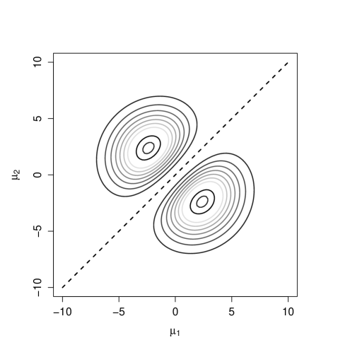
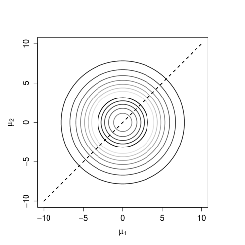
Figure 1. Default MOM-IW $p(\mu_{1},\mu_{2}\mid\sigma^{2}=1,g=5.68,\mathcal{M}_{2})$ (left) and Normal-IW $p^{L}(\mu_{1},\mu_{2}\mid\sigma^{2}=1,g^{L}=11.56,\mathcal{M}_{2})$ (right)

We start by discussing $g$, first for Normal and T mixtures and subsequently for Binomial and product Binomial mixtures. The main idea for Normal and T mixtures is that we wish to find clearly-separated components, so we can interpret the data-generating process in terms of distinct sub-populations. We thus set $g$ such that there is small prior probability that any two components are poorly-separated, i.e. give rise to a unimodal density. In Normal mixtures the number of modes depends on non-trivial parameter combinations (Ray and Lindsay, 2005), but when $\eta_{1}=\eta_{2}=0.5$ and $\Sigma_{1}=\Sigma_{2}$ the mixture is bimodal if and only if $\kappa=(\bm{\mu}_{1}-\bm{\mu}_{2})^{{}^{\prime}}\Sigma^{-1}(\bm{\mu}_{1}-\bm{\mu}_{2})>4$. Thus we set $g$ such that $P(\kappa<4\mid\mathcal{M}_{2})=0.05$. This is trivial, the prior on $\kappa$ implied by (2.4) is $p(\kappa\mid\mathcal{M}_{2})=\text{Gamma}(\kappa;p/2+1,1/(4g))$. For instance in a univariate Normal mixture $g=5.68$, Figure 1 (left) portrays the associated prior. For comparison the right panel shows a Normal prior with $g^{L}=11.56$, which also assigns $P^{L}(\kappa<4\mid\mathcal{M}_{2})=0.05$. To assess sensitivity we considered $g$ such that $P(\kappa<4\mid\mathcal{M}_{2})=0.1$, finding that $P(\kappa<4\mid\mathcal{M}_{2})=0.05$ is slightly preferable for balancing parsimony vs. sensitivity (Supplementary Section S12).

For T mixtures Došlá (2009) showed that a univariate mixture with two components and equal degrees of freedom $\upsilon$ is bimodal if $\kappa>4\upsilon/(\upsilon+2)$. For multivariate T mixtures, again with $\eta_{1}=\eta_{2}=0.5$ and $\Sigma_{1}=\Sigma_{2}$, it is easy to develop the arguments in Ray and Lindsay (2005) (Theorem 1 and Remark 4) to show that the mixture is bimodal if and only if $\kappa>4\upsilon/(\upsilon+p+1)$. This matches the result from Došlá (2009) for $p=1$ and for Normal mixtures in Ray and Lindsay (2005) as $\upsilon\rightarrow\infty$. Summarising, we set $g$ such that $P(\kappa<4\upsilon/(\upsilon+p+1)\mid\upsilon,\mathcal{M}_{k})=0.05$, where we recall that $p(\kappa\mid\upsilon,\mathcal{M}_{2})=\text{Gamma}(\kappa;p/2+1,1/(4g))$.

Consider now the MOM-Beta prior (2.6). In contrast to continuous mixtures here one cannot use multi-modality to set the prior parameters $(a,g)$. Instead we set $(a,g)$ such that the amount of prior information (measured by the variance) is comparable to that in

(2.9) $$p^{L}(\bm{\theta}\mid\mathcal{M}_{k})=\prod_{j=1}^{k}\prod_{f=1}^{p}\mbox{Beta}(\theta_{jf};g_{L}a_{L},g_{L}(1-a_{L})),$$

where $a_{L}=0.5$ and $g_{L}=2$ are typically viewed as minimally informative. Specifically we recommend $a=0.5$ and $g$ as listed in Table S1 for $p\in[1,20]$, and $g=2$ for $p>20$. We briefly outline the reasoning, further details are in Supplementary Section S3. Simple algebra shows that the variance under $p^{L}$ is

$$\mbox{Var}_{p^{L}}(\theta_{jf}-\theta_{j^{\prime}f}\mid\mathcal{M}_{k})=2\left[\frac{a_{L}(g_{L}a_{L}+1)}{g_{L}+1}-a_{L}^{2}\right],$$

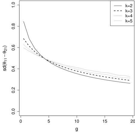
Figure S2. Prior standard deviation $\mbox{SD}(\theta_{11}-\theta_{21}\mid\mathcal{M}_{k})$ under a MOM-Beta$(0.5g,0.5(1-g))$

and for $(a_{L},g_{L})=(0.5,2)$ this variance is 1/6. We seek $g$ such that the variance under the MOM-Beta prior $\mbox{Var}_{p}(\theta_{jf}-\theta_{j^{\prime}f}\mid\mathcal{M}_{k})=1/6$. Although such $g$ depends on $(k,p)$ the dependence on $k$ is mild (in fact for large $k$ the variance grows less sensitive to $g$, Figure S2) and one can focus on the $k=2$ case. See Supplementary Section S3 for the variance under general $(a,g)$ and $k=2$. Interestingly as $p$ grows one may simply set $(a,g)=(0.5,2)$, since then

$$\mbox{Var}_{p}(\theta_{jf}-\theta_{j^{\prime}f}\mid\mathcal{M}_{2})=\frac{1}{p}\left(\frac{2}{5}+\frac{p-1}{6}\right),$$

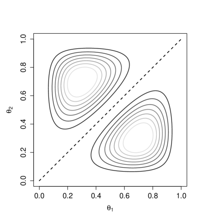
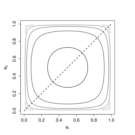
Figure S1. Default MOM-Beta ($a=0.5$, $g=7.11$) (left) and Beta(1,1) (right)

which converges to $1/6$ as $p\rightarrow\infty$, thus for large $p$ one may simply set $g=2$. Figure S1 displays the default MOM-Beta and Beta(1,1) priors for $k=2$. See also Section S6 for an illustration of the sensitivity of results to various $g$ in an application.

Regarding $q$, as discussed earlier $q>1$ is required for (2.3) to define a NLP. One option is to set $q=3$ so that $p(\bm{\eta}\mid\mathcal{M}_{k})\propto\prod_{j=1}^{k}\eta_{j}^{2}$ induces a quadratic penalty comparable to the MOM prior on $\bm{\mu}$ given in (2.4). Alternatively from the discussion after Proposition 1 setting $q=(p_{k}-p_{k^{*}})/(k-k^{*})$, the number of parameters per component, seeks to (at least) double the Bayes factor sparsity rate of the underlying LP. For instance, for Normal mixtures with common covariances this leads to $q=p+1$, and under unequal covariances to $q=p+0.5p(p+1)+1$. These are the values we used in our examples with $p=1$ or $p=2$ (Section 4), but we remark that for larger $p$ such $q$ may lead to an overly informative prior on $\bm{\eta}$. In our experience $q\in[2,4]$ (Supplementary Section S12) gives fairly robust results and satisfactory sparsity, thus larger values do not seem warranted.

The prior distribution on the remaining parameters, which may be thought of as nuisance parameters, will typically reduce to a standard form for which defaults are available. For example, for location-scale mixtures we set $p(\Sigma_{1},\ldots,\Sigma_{k}\mid\mathcal{M}_{k})=\prod_{j=1}^{k}\mbox{IW}(\Sigma_{j};\nu,S)$. We follow the recommendation in Hathaway (1985) that eigenvalues of $\Sigma_{i}\Sigma_{j}^{-1}$ for any $i\neq j$ should be bounded away from 0 to prevent the posterior from becoming unbounded, which is achieved if $\nu\geq p+4$ (Frühwirth-Schnatter, 2006, Ch. 6). We assume that the data are standardized to have mean 0 and variance 1 and set a default $S=(p+4)^{-1}I$ and $\nu=p+4$, so that $E(\Sigma_{j}^{-1})=I$. For T mixtures, we also consider a prior the degrees of freedom $\upsilon$. We refer to Rossell and Steel (2018) for a review of popular options.

3. Computational algorithms

Computation for mixtures is challenging, and potentially more so when embarking upon non-standard formulations such as ours. Fortunately, Theorem 1(i) allows estimating the integrated likelihood $p({\bf y}\mid\mathcal{M}_{k})$ for arbitrary mixtures through direct extensions of existing algorithms. Intuitively, one can use any algorithm to estimate a local prior integrated likelihood $\tilde{p}({\bf y}\mid\mathcal{M}_{k})$ and the mean of $d_{\vartheta}(\bm{\vartheta}_{k})$ under the local posterior. In Section 3.1 we outline the main idea. Section 3.2 gives two algorithms to estimate $\tilde{p}({\bf y}\mid\mathcal{M}_{k})$ from MCMC output. The first one was proposed by Marin and Robert (2008) and, while we found it to be reasonably accurate, it is limited to conjugate models and requires an MCMC post-processing step that can have non-negligible cost. The second algorithm is novel (to our knowledge), applicable to non-conjugate models and only requires cluster probabilities readily available as an MCMC by-product. This algorithm is based on a novel result connecting Bayes factors with the ratio of posterior to prior empty cluster probabilities, i.e. a type of Savage-Dickey ratio, hence we named it the empty cluster probability (ECP) estimator. We found that in some situations the ECP estimator can increase precision by an order of magnitude relative to that in Marin and Robert (2008) (Supplementary Section S7, Figures S4-S5) using the same number of MCMC iterations. Further, as explained below the ECP estimator can have a substantially smaller per-iteration cost. We remark that the result has interest beyond purely computational purposes, e.g. to set thresholds on empty cluster probabilities in overfitted mixtures. Also note that computations are easily done in parallel, e.g. to consider multiple $k$ or process MCMC output in batches. See Section 4.1 for further discussion and empirical results on the run time required by our algorithms. Although our main interest is to infer $k$, in Section 3.3 we discuss posterior mode parameter estimates via an Expectation-Maximimation (EM) algorithm (Dempster et al. (1977)). Relative to local priors the EM algorithm only requires an extra gradient evaluation, which typically has negligible cost.

3.1. Approximation of $p({\bf y}\mid\mathcal{M}_{k})$

Theorem 1(i) suggests the estimator

(3.1) $$\hat{p}({\bf y}\mid\mathcal{M}_{k})=\tilde{p}({\bf y}\mid\mathcal{M}_{k})\dfrac{1}{T}\sum_{t=1}^{T}\omega(\bm{\vartheta}_{k}^{(t)}),$$

where $\omega(\bm{\vartheta}_{k})=p(\bm{\vartheta}_{k}\mid\mathcal{M}_{k})/\tilde{p}(\bm{\vartheta}_{k}\mid\mathcal{M}_{k})$ and $\tilde{p}(\bm{\vartheta}_{k}\mid\mathcal{M}_{k})$ is an arbitrary LP conveniently chosen so that MCMC algorithms to sample $\bm{\vartheta}_{k}^{(t)}\sim\tilde{p}(\bm{\vartheta}_{k}\mid{\bf y},\mathcal{M}_{k})\propto p({\bf y}\mid\bm{\vartheta}_{k},\mathcal{M}_{k})\tilde{p}(\bm{\vartheta}_{k}\mid\mathcal{M}_{k})$ are readily available. See Supplementary Section S9 for standard Gibbs algorithms for Normal and product Binomial mixtures. For the MOM-IW in (2.4) we used

$$\tilde{p}(\bm{\vartheta}_{k}\mid\mathcal{M}_{k})=\text{Dir}(\bm{\eta};q)\prod_{j=1}^{k}N\left(\bm{\mu}_{j}\mid\bm{0},g\Sigma_{j}\right)\text{IW}(\Sigma_{j}\mid\nu,S),$$

with $q>1$, which gives

$$\omega(\bm{\vartheta}_{k})=\dfrac{1}{C_{k}}\prod_{1\leq i<j\leq k}\frac{(\bm{\mu}_{i}-\bm{\mu}_{j})^{{}^{\prime}}A_{\Sigma}^{-1}(\bm{\mu}_{i}-\bm{\mu}_{j})}{g}\prod_{j=1}^{k}\frac{N(\bm{\mu}_{j}\mid{\bf 0},gA_{\Sigma})}{N(\bm{\mu}_{j}\mid{\bf 0},g\Sigma_{j})}.$$

For the MOM-Beta in (2.6) we used $\tilde{p}(\bm{\vartheta}_{k}\mid\mathcal{M}_{k})=\text{Dir}(\bm{\eta};q)\prod_{j=1}^{k}\prod_{f=1}^{p}\text{Beta}(\theta_{jf};ag,(1-a)g)$, hence

$$\omega(\bm{\vartheta}_{k})=\frac{1}{C_{k}}\prod_{1\leq i<j\leq k}(\bm{\theta}_{i}-\bm{\theta}_{j})^{\prime}(\bm{\theta}_{i}-\bm{\theta}_{j}).$$

Our strategy is admittedly simple but has convenient advantages. After obtaining $\tilde{p}({\bf y}\mid\mathcal{M}_{k})$ one need only compute a posterior average. Furthermore, only posterior sampling under $\tilde{p}(\bm{\vartheta}_{k}\mid{\bf y},\mathcal{M}_{k})$ is required. As a caveat the posterior variance of $\omega(\bm{\vartheta}_{k})$ has an effect on $\hat{p}({\bf y}\mid\mathcal{M}_{k})$, specifically when the local and non-local posteriors differ substantially this variance can potentially be large. However from Theorem 1 these posteriors differ mainly in overfitted mixtures ($k>k^{*}$), and only the numerator but not the denominator in $\omega(\bm{\vartheta}_{k})$ may vanish (provided $\tilde{p}$ is positive over its domain, as is the case), hence in practice we found (3.1) to be quite stable (Supplementary Section S8). We remark that $\omega(\bm{\vartheta}_{k})$ is not a reweighting to convert samples from $\tilde{p}(\bm{\vartheta}_{k}\mid{\bf y},\mathcal{M}_{k})$ into samples from $p(\bm{\vartheta}_{k}\mid{\bf y},\mathcal{M}_{k})$, but a direct approximation to the posterior mean of $d(\bm{\vartheta}_{k})$ under $\tilde{p}(\bm{\vartheta}\mid{\bf y},\mathcal{M}_{k})$. However, if interested in posterior samples from $p(\bm{\vartheta}_{k}\mid{\bf y},\mathcal{M}_{k})$ one could clearly use such a reweighting. Alternatively one can devise a sampler directly for the non-local $p(\bm{\vartheta}_{k}\mid{\bf y},\mathcal{M}_{k})$, e.g. using slice sampling (Petralia et al., 2012), latent truncations (Rossell and Telesca, 2017) or collapsed Gibbs (Xie and Xu, 2019), but we do not pursue this as our main interest is model selection.

3.2. Approximation of $\tilde{p}({\bf y}\mid\mathcal{M}_{k})$

There are a number of proposals to estimate $\tilde{p}({\bf y}\mid\mathcal{M}_{k})$ in the literature, e.g. trans-dimensional MCMC (Richardson and Green, 1997), Bridge sampling (Frühwirth-Schnatter, 2004), dual importance sampling (Lee and Robert, 2016) and collapsed Gibbs sampling (Xie and Xu, 2019). Each of these has its own set of advantages and limitations, but ultimately obtaining $\tilde{p}({\bf y}\mid\mathcal{M}_{k})$ in a truly scalable fashion remains an open problem.

We focus on two algorithms that are simple to implement and we found to attain a good cost versus precision tradeoff. We denote by $z_{i}\in\{1,\ldots,k\}$ the latent cluster indicators, i.e. $z_{i}=j$ if observation $i$ is assigned to component $j$, ${\bf z}=(z_{1},\ldots,z_{n})$ and $n_{j}=\sum_{i=1}^{n}\mbox{I}(z_{i}=j)$ is the number of individuals in cluster $j$. The first algorithm is a refinement proposed by Marin and Robert (2008) of an algorithm by Chib (1995). The strategy uses the identity

(3.2) $$\tilde{p}({\bf y}\mid\mathcal{M}_{k})=\frac{p({\bf y}\mid\hat{\bm{\vartheta}}_{k},\mathcal{M}_{k})\tilde{p}(\hat{\bm{\vartheta}}_{k}\mid\mathcal{M}_{k})}{\tilde{p}(\hat{\bm{\vartheta}}_{k}\mid{\bf y},\mathcal{M}_{k})}=\frac{p({\bf y}\mid\hat{\bm{\vartheta}}_{k},\mathcal{M}_{k})\tilde{p}(\hat{\bm{\vartheta}}_{k}\mid\mathcal{M}_{k})}{\sum_{\psi\;\in\;\mathfrak{N}(k)}\tilde{p}(\psi(\hat{\bm{\vartheta}}_{k})\mid{\bf y},\mathcal{M}_{k})/(k!)},$$

where $\hat{\bm{\vartheta}}_{k}$ is the posterior mode and $\mathfrak{N}(k)$ the set of $k!$ possible permutations of $\{1,...,k\}$. The right-hand side holds for exchangeable $\tilde{p}(\bm{\vartheta}_{k}\mid\mathcal{M}_{k})$, as then the posterior is invariant to label-switching. The numerator in (3.2) simply requires evaluating the likelihood and prior at $\hat{\bm{\vartheta}}_{k}$. Marin and Robert (2008) propose estimating the denominator by

(3.3) $$\dfrac{1}{Tk!}\sum_{\psi\;\in\;\mathfrak{N}(k)}\sum_{t=1}^{T}\tilde{p}(\psi(\hat{\bm{\vartheta}}_{k})\mid{\bf y},{\bf z}^{(t)},\mathcal{M}_{k}),$$

where ${\bf z}^{(t)}=(z_{1}^{(t)},\ldots,z_{n}^{(t)})$ are samples from $\tilde{p}({\bf z},\bm{\vartheta}_{k}\mid{\bf y},\mathcal{M}_{k})$. The estimator (3.2)-(3.3) can be applied as long as the posterior density $\tilde{p}(\psi(\hat{\bm{\vartheta}}_{k})\mid{\bf y},{\bf z}^{(t)},\mathcal{M}_{k})$ has closed-form, e.g. in conjugate models. Specifically for Normal mixtures

$$\tilde{p}(\psi(\hat{\bm{\vartheta}}_{k})\mid{\bf y},\bm{z}^{(t)},\mathcal{M}_{k}) =\prod_{j=1}^{k}N\left(\psi(\hat{\bm{\mu}}_{j});\frac{gn_{j}^{(t)}\bar{{\bf y}}_{j}^{(t)}}{1+gn_{j}^{(t)}},\dfrac{g}{1+gn_{j}^{(t)}}\Sigma_{j}^{(t)}\right)\text{IW}\left(\psi(\hat{\Sigma}_{j});\nu+n_{j}^{(t)},S_{j}^{(t)}\right)$$

$$\times\text{Dir}(\psi(\hat{\bm{\eta}});q+n_{1}^{(t)},...,q+n_{k}^{(t)}),$$

and for product Binomial mixtures

$$\tilde{p}(\psi(\hat{\bm{\vartheta}}_{k})\mid{\bf y},\bm{z}^{(t)},\mathcal{M}_{k})= \prod_{j=1}^{k}\prod_{f=1}^{p}\text{Beta}\left(\psi(\hat{\theta}_{jf});ag+\sum_{z_{i}^{(t)}=j}y_{if},(1-a)g+\sum_{z_{i}^{(t)}=j}(L_{if}-y_{if})\right)$$

$$\times\text{Dir}(\psi(\hat{\bm{\eta}});q+n_{1}^{(t)},...,q+n_{k}^{(t)}).$$

We now outline our ECP algorithm, which relies on Proposition 1 below expressing Bayes factors as a ratio of posterior to prior empty cluster probabilities. This representation can be viewed as a Savage-Dickey probability ratio, a natural extension of the familiar density ratio. The result applies to any mixture and prior satisfying the minimal conditions C1-C4 below. In the remainder of this section $p(\bm{\vartheta}_{k}\mid\mathcal{M}_{k})$ denotes an arbitrary prior for which one wants to obtain posterior model probabilities, e.g. in our examples this is the local prior $\tilde{p}(\bm{\vartheta}_{k}\mid M_{k})$ and then non-local posterior probabilities are obtained from (3.1).

1. Conditional independence. $p({\bf y}\mid{\bf z},\bm{\vartheta}_{k},\mathcal{M}_{k})=\prod_{j=1}^{k}\prod_{z_{i}=j}p({\bf y}_{i}\mid\bm{\theta}_{j},\mathcal{M}_{k})$

2. Invariance to label permutations. $p({\bf y}\mid\bm{\vartheta}_{k})=p({\bf y}\mid\psi(\bm{\vartheta}_{k}))$ and $p({\bf z}\mid\mathcal{M}_{k})=p(\varrho({\bf z})\mid\mathcal{M}_{k})$ for any permutation of component parameters $\psi$ and component indexes $\varrho$.

3. Coherence of prior on cluster allocations. $p({\bf z}\mid n_{k}=0,\mathcal{M}_{k})=p({\bf z}\mid\mathcal{M}_{k-1})$

4. Coherence of prior on parameters. For any $\bm{\theta}_{1},\ldots,\bm{\theta}_{k-1}$ and any ${\bf z}$ such that $n_{k}=0$, it holds that

   $$p(\bm{\theta}_{1},\ldots,\bm{\theta}_{k-1}\mid{\bf z},\mathcal{M}_{k-1})=\int p(\bm{\theta}_{1},\ldots,\bm{\theta}_{k},\mid{\bf z},\mathcal{M}_{k})d\bm{\theta}_{k}$$

Conditions C1-C2 hold for the vast majority of mixtures, including mixtures of regressions and most hidden Markov models. Conditions C3-C4 hold for most common priors. For instance C3 holds when $p(\bm{\eta}\mid\mathcal{M}_{k})$ and $p(\bm{\eta}\mid\mathcal{M}_{k-1})$ are both symmetric Dir$(q)$ distributions and C4 is satisfied by priors that factor across components, e.g. $p(\bm{\vartheta}_{k}\mid\mathcal{M}_{k})=\mbox{Dir}(\bm{\eta};q)\prod_{j=1}^{k}p(\bm{\theta}_{j}\mid\mathcal{M}_{k})$.

Proposition 1.

Suppose that C1-C4 hold. Then the Bayes factor for ${\mathcal{M}_{k-1}}$ versus $\mathcal{M}_{k}$ is

$$B_{k-1,k}({\bf y})=\frac{\sum_{j=1}^{k}P(n_{j}=0\mid{\bf y},\mathcal{M}_{k})/k}{P(n_{j}=0\mid\mathcal{M}_{k})}.$$

Once $B_{k-1,k}({\bf y})$ for $k\in\{2,\ldots,K\}$ are available then $P(\mathcal{M}_{k}\mid{\bf y})$ are obtained as usual. Proposition 1 is easy to implement, e.g. if $p(\bm{\eta}\mid M_{j})=\mbox{Dir}(\bm{\eta};q)$ for all $j$ then

$$P(n_{j}=0\mid\mathcal{M}_{k})=\frac{\Gamma(kq)\Gamma(n+(k-1)q)}{\Gamma((k-1)q)\Gamma(n+kq)}.$$

Further, given draws $\bm{\vartheta}_{k}^{(t)}\sim p(\bm{\vartheta}_{k}\mid{\bf y},\mathcal{M}_{k})$ one can obtain Rao-Blackwellised estimates

(3.4) $$\hat{P}(n_{j}=0\mid{\bf y},\mathcal{M}_{k})=\frac{1}{T}\sum_{t=1}^{T}P(n_{j}=0\mid{\bf y},\bm{\vartheta}_{k}^{(t)},\mathcal{M}_{k})=\frac{1}{T}\sum_{t=1}^{T}\prod_{i=1}^{n}P(z_{i}\neq j\mid{\bf y},\bm{\vartheta}_{k}^{(t)},\mathcal{M}_{k}).$$

That is, the Bayes factor under local priors $\tilde{B}_{k-1,k}({\bf y})$ is obtained dividing (3.4) by $P(n_{j}=0\mid\mathcal{M}_{k})$. To estimate Bayes factors under NLPs $\hat{B}_{k-1,k}({\bf y})$ we use the estimator in 3.1

$$\hat{B}_{k-1,k}({\bf y})=\tilde{B}_{k-1,k}({\bf y})\dfrac{\sum_{t=1}^{T}\omega(\bm{\vartheta}_{k-1}^{(t)})}{\sum_{t=1}^{T}\omega(\bm{\vartheta}_{k}^{(t)})},$$

Note that ECP only requires cluster probabilities, hence it remains valid for non-conjugate models.

Proposition 1 is of independent interest to help discard unoccupied clusters in overfitted mixtures. It suggests that the threshold on posterior empty cluster probabilities should depend on the corresponding prior empty cluster probabilities. The latter are a function of $n$, $k$ and $q$, hence using fixed thresholds may be suboptimal. Note also that Proposition 1 can be used to compare structurally different models. For instance let $B_{k1}$ be the Bayes factor between a $k$-component unequal-covariance Normal mixture vs. a one-component Normal, and $B^{c}_{k1}$ that for a $k$-component common-covariance Normal mixture vs. a one-component Normal. Then $B_{k1}/B^{c}_{k1}$ is the Bayes factor comparing $k$ components with unequal vs. equal covariances. Similarly one could combine the Bayes factor between a one-component Normal vs. a one-component T (which is easy to compute) with Proposition 1 to obtain Bayes factors between any $k$-component Normal vs. T mixture. That is, the ECP estimator is connected to empty cluster probabilities but really is a tool to obtain $P(\mathcal{M}_{k}\mid{\bf y})$ and hence remains applicable in more general settings.

3.3. Posterior modes

The EM algorithm provides a fast way to obtain posterior modes $\hat{\bm{\vartheta}}_{k}=\arg\max_{\bm{\vartheta}_{k}}p(\bm{\vartheta}_{k}\mid{\bf y},\mathcal{M}_{k})$ or cluster assigments $\hat{z}_{i}=\arg\max_{j\in\{1,\ldots,K\}}p(z_{i}=j\mid{\bf y},\hat{\bm{\vartheta}}_{k},\mathcal{M}_{k})$. This optimization problem is conceptually related to maximizing a penalized likelihood, e.g. setting fused LASSO penalties on the separation between means (Heinzl and Tutz, 2014), although we remark that the latter shrink components closer to each other rather than pushing them apart as is the case for non-local priors.

We briefly describe our algorithm, which is derived in Supplementary Sections S10 and S11. At iteration $t$ the E-step computes

$$\bar{z}_{ij}^{(t)}=P(z_{i}=j\mid{\bf y}_{i},\bm{\vartheta}_{j}^{(t-1)})=\eta_{j}^{(t-1)}p({\bf y}_{i}\mid\bm{\theta}_{j}^{(t-1)})/\sum_{j=1}^{k}\eta_{j}^{(t-1)}p({\bf y}_{i}\mid\bm{\theta}_{j}^{(t-1)})$$

and is trivial to implement. The M-step requires updating $\bm{\vartheta}_{k}^{(t)}$ in a manner that increases the expected complete log-posterior, which we denote by $\xi(\bm{\vartheta}_{k})$, but under our prior $p(\bm{\vartheta}_{k}\mid\mathcal{M}_{k})=d_{\vartheta}(\bm{\vartheta}_{k})\tilde{p}(\bm{\vartheta}_{k}\mid\mathcal{M}_{k})$ this cannot be done in closed-form. A key observation is that if $\tilde{p}(\bm{\vartheta}_{k}\mid\mathcal{M}_{k})$ leads to closed-form updates, the corresponding target $\tilde{\xi}(\bm{\vartheta}_{k})$ only differs from $\xi(\bm{\vartheta}_{k})$ by a term $d_{\vartheta}(\bm{\vartheta}_{k})$, thus one may approximate $\xi(\bm{\vartheta}_{k})$ via a first order Taylor expansion of $d_{\vartheta}(\bm{\vartheta}_{k})$. These approximate updates need not lead to an increase in $\xi(\bm{\vartheta}_{k})$ (although they typically do since $d_{\vartheta}(\bm{\vartheta}_{k})$ has a mild influence for moderately large $n$), and whenever this happens we use gradient algorithm updates. Algorithms 1 and S5 detail the steps for Normal and product Binomial mixtures (extensions to other models follow similar lines), for simplicity outlining the approximate updates (see Supplementary Section S10 for the gradient algorithm). In our implementation we initialize $\bm{\vartheta}_{k}^{(0)}$ to the MLE and stop when the increase in $\xi(\bm{\vartheta}_{k})$ is below a tolerance $\epsilon^{*}=0.0001$ or a maximum number of iterations $T=10,000$ is reached. For ease of notation in Algorithm 1 we define $d_{ij}=(\bm{\mu}_{i}-\bm{\mu}_{j})^{\prime}A_{\Sigma}^{-1}(\bm{\mu}_{i}-\bm{\mu}_{j})$ evaluated at the current value of $\bm{\mu}_{1},\ldots,\bm{\mu}_{k},\Sigma_{1},\ldots,\Sigma_{k}$.

Set $t=1$. while $\zeta>\epsilon^{*}$ and $t<T$ do

       for $t\geq 1$ and $j=1,...,k$ do

             E-step. Let $\bar{z}^{(t)}_{ij}=\dfrac{\eta_{j}^{(t-1)}N({\bf y}_{i};\bm{\mu}_{j}^{(t-1)},\Sigma_{j}^{(t-1)})}{\sum_{j=1}^{k}\eta_{j}^{(t-1)}N({\bf y}_{i};\bm{\mu}_{j}^{(t-1)},\Sigma_{j}^{(t-1)})}$ and $n_{j}^{(t)}=\sum_{i=1}^{n}\bar{z}^{(t)}_{ij}$.

            M-step. Let $\bar{{\bf y}}_{j}^{(t)}=\sum_{i=1}^{n}\bar{z}^{(t)}_{ij}{\bf y}_{i}/n_{j}^{(t)}$. Update

$$\bm{\mu}_{j}^{(t)}=\left(\left(\Sigma_{j}^{-1}\right)^{(t-1)}n_{j}^{(t)}+A_{\Sigma^{(t-1)}}^{-1}\left(\dfrac{1}{g}+\sum_{\begin{subarray}{c}i\neq j\end{subarray}}\frac{2}{d_{ij}}\right)\right)^{-1}$$

$$\times\left(\Sigma^{-1(t-1)}n_{j}^{(t)}\bar{{\bf y}}_{j}^{(t)}+A_{\Sigma^{(t-1)}}^{-1}\left(\sum_{\begin{subarray}{c}i\neq j\end{subarray}}\frac{\bm{\mu}_{j}^{(t-1)}-(\bm{\mu}_{i}^{(t-1)}-\bm{\mu}_{j}^{(t-1)})}{d_{ij}}\right)\right),$$

            Update $(\nu-p+n_{j}^{(t)})\Sigma^{(t)}_{j}=$

$$S^{-1}+\dfrac{\bm{\mu}_{j}^{(t)}(\bm{\mu}_{j}^{(t)})^{\prime}}{kg}+\sum_{i=1}^{n}\bar{z}^{(t)}_{ij}({\bf y}_{i}-\bm{\mu}_{j}^{(t)})({\bf y}_{i}-\bm{\mu}_{j}^{(t)})^{{}^{\prime}}-\dfrac{1}{k}\sum_{\begin{subarray}{c}i\neq j\end{subarray}}\dfrac{2(\bm{\mu}_{j}^{(t)}-\bm{\mu}_{k}^{(t)})(\bm{\mu}_{j}^{(t)}-\bm{\mu}_{k}^{(t)})^{{}^{\prime}}}{d_{ij}}.$$

Update $\eta^{(t)}_{j}=\dfrac{n_{j}^{(t)}+q-1}{n+k(q-1)}$.

       end for

      Compute $\zeta=|\xi(\bm{\vartheta}_{k}^{(t)})-\xi(\bm{\vartheta}_{k}^{(t-1)})|$ and set $t=t+1$.

end while

Algorithm 1 EM under MOM-IW-Dir priors.

4. Empirical Results

We compared our MOM-IW-Dir and MOM-Beta-Dir priors with default parameters (Section 2.3) to their local counterparts, Normal-IW-Dir and Beta(1,1)-Dir respectively. As described in Section 2.3 the Normal-IW-Dir prior parameter $g^{L}$ was set to match the 95% percentile for the separation parameter $\kappa$. Throughout we use uniform model priors $P(\mathcal{M}_{j})=1/K,j=1\dots,K$. Unless otherwise stated we estimated the integrated likelihoods using Algorithm S2 and S3 based on 5,000 MCMC draws after a 2,500 burn-in. We also considered the BIC, AIC, sBIC, overfitted mixtures and repulsive overfitted mixtures. We only found an sBIC implementation for Normal mixture with $\Sigma_{i}\neq\Sigma_{j}$. For Normal mixtures we used the function GaussianMixtures and for Binomial mixtures we used the function BinomialMixtures from the R package sBIC (Weihs and Plummer, 2016). In GaussianMixtures we used the default real canonical threshold value given by $\lambda\leq\frac{1}{2}(jd+j-1+(k-j)\varphi)$ with $\varphi$ chosen in relation to a prior on mixture weights and we denote this by sBIC. In BinomialMixtures we tried two sBIC versions, named $\overline{\text{sBIC}}$ and $\overline{\text{sBIC}}_{05}$ corresponding to setting the real canonical threshold to $\lambda\leq\frac{1}{2}(k+j-1)$ and $\lambda\leq\frac{1}{4}(j+3k)-\frac{1}{2}$ respectively.

In Sections 4.1-4.6 we use Normal mixtures. Section 4.1 presents a simulation study for univariate and bivariate Normal mixtures. Section 4.2 explores model misspecification by simulating data from T mixtures. In Sections 4.3-4.5 we analyse several datasets, including a flow cytometry experiment and Fisher’s Iris data for which there is a known ground truth. Section 4.6 offers a comparison to applying overfitted mixtures to these datasets. Section 4.7 reproduces a Binomial mixture example used by Drton and Plummer (2017) to illustrate the sBIC, and Section 4.8 analyses a US political blog dataset via product Binomial mixtures. We used R package NLPmix for the EM algorithm and the estimate $\hat{p}({\bf y}\mid\mathcal{M}_{k})$ from Marin and Robert (2008), and for our ECP estimator we used bfnormmix from R package mombf. As illustration, the code for a simulation in Section 4.1 is provided in Supplementary Section S14 and that for Section 4.2 in a supplementary file. See also Supplementary Section S15 for a simulation experiment for product Binomial mixtures to illustrate the usage of diagnostics for multiple EM and MCMC runs.

4.1. Simulation study with Normal mixtures

We consider choosing amongst the three competing models

$$\mathcal{M}_{1} :N({\bf y}_{i};\bm{\mu},\Sigma),$$

$$\mathcal{M}_{2} :\eta_{1}N({\bf y}_{i};\bm{\mu}_{1},\Sigma)+(1-\eta_{1})N({\bf y}_{i};\bm{\mu}_{2},\Sigma)$$

$$\mathcal{M}_{3} :\eta_{1}N({\bf y}_{i};\bm{\mu}_{1},\Sigma)+\eta_{2}N({\bf y}_{i};\bm{\mu}_{2},\Sigma)+(1-\eta_{1}-\eta_{2})N({\bf y}_{i};\bm{\mu}_{3},\Sigma),$$

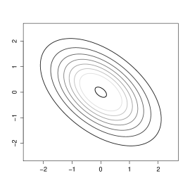
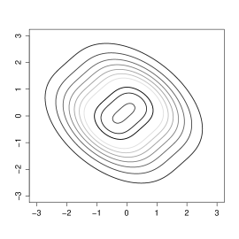
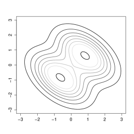
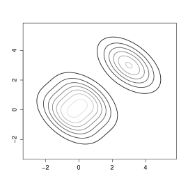
Figure S9. Simulation study data-generating truth. Case 1: $k^{*}$=1, $\bm{\mu}_{1}$=0; Case 2: $k^{*}$=2, $\bm{\mu}_{1}$=-1, $\bm{\mu}_{2}$=1, $\bm{\eta}=(0.5,0.5)$; Case 3: $k^{*}$=2, $\bm{\mu}_{1}=-2,\bm{\mu}_{2}=2$, $\bm{\eta}$=0.5; Case 4: $k^{*}$=3, $\bm{\mu}_{1}=-1,\bm{\mu}_{2}=1,\bm{\mu}_{3}=4$, $\bm{\eta}=$(0.45,0.45,0.1); Case 5: $k^{*}$=1, $\bm{\mu}=(0,0)^{\prime}$; Case 6: $k^{*}$=2, $\bm{\mu}_{1}=(-0.4,-0.6)^{\prime}$, $\bm{\mu}_{2}=-\bm{\mu}_{1}$; Case 7: $k^{*}$=2, $\bm{\mu}_{1}=(-0.65,-0.85)^{\prime}$, $\bm{\mu}_{2}=-\bm{\mu}_{1}$; Case 8: $k^{*}$=3, $\bm{\mu}_{1}=(-0.65,-0.85)^{\prime}$, $\bm{\mu}_{2}=-\bm{\mu}_{1}$, $\bm{\mu}_{3}=(3,3)^{\prime}$, $\bm{\eta}$=(0.35,0.35,0.3). $\Sigma=1$ in Cases 1-4, $\sigma^{2}_{11}=\sigma^{2}_{22}=1$ and $\sigma^{2}_{12}=\sigma^{2}_{21}=-0.5$ in Cases 5-8.

where independence is assumed across $i=1,\ldots,n$. We simulated 100 datasets under each of the 8 data-generating truths with Normal components depicted in Figure S9 for univariate (Cases 1-4) and bivariate outcomes (Cases 5-8). Case 1 corresponds to $k^{*}=1$ components, Cases 2-3 to $k^{*}=2$ moderately and strongly-separated components respectively, and Case 4 to $k^{*}=3$ with two strongly overlapping components and a third component with smaller weight. Cases 5-8 are analogous for the bivariate outcome.

Figure 2 shows the average posterior probability assigned to the data-generating model $P(\mathcal{M}_{k^{*}}\mid{\bf y})$ as a function of $n$ under NLP and LP. To compare frequentist and Bayesian methods Figure 3 reports the (frequentist) proportion of correct model selections, i.e. the proportion of simulated datasets in which $\hat{k}=k^{*}$, where $\hat{k}$ is the selected number of components by any given method (for Bayesian methods $\hat{k}=\arg\max_{k}p(\mathcal{M}_{k}\mid{\bf y})$).

Case 1	Case 2
Case 3	Case 4
Case 5	Case 6
Case 7	Case 8

Figure 2. Simulation study. $P(\mathcal{M}_{k^{*}}\mid{\bf y})$ versus $n$ for the MOM-IW (solid line) and Normal-IW (dashed line).

Case 1	Case 2
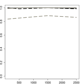
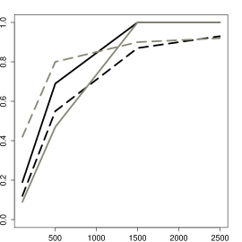
Case 3	Case 4
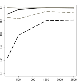
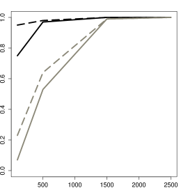
Case 5	Case 6
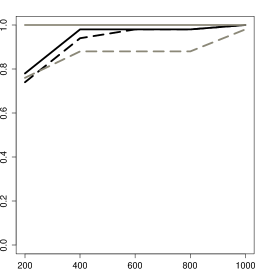
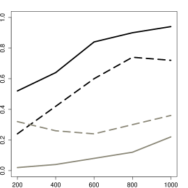
Case 7	Case 8

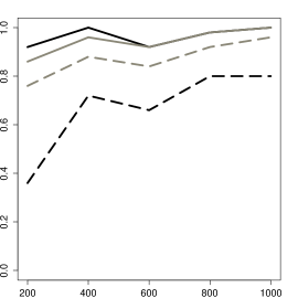
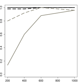
Figure 3. Simulation study. Proportion of correct $\hat{k}=k$ vs. $n$ for MOM-IW (solid black), Normal-IW (dashed black), AIC (dashed gray) and BIC (solid gray)

Figures S10-S12 show the corresponding posterior expected model size $E(k\mid{\bf y})$ and average $\hat{k}$. For $E(k\mid{\bf y})$ we set $q=p+1$ as the default prior specification of $q$ and we perform a sensitivity prior analysis (Subsection 2.3) with another $q$ suggested in Frühwirth-Schnatter (2006). Figure S13 plots $P(\mathcal{M}_{k^{*}}\mid{\bf y})$ setting $g$ so that $P(\kappa<4\mid\mathcal{M}_{k})=0.1$ instead of 0.05. Overall a similar behavior is observed in the univariate and bivariate cases. The BIC adequately favoured sparse solutions (Cases 1,3,5,7) but showed an important lack of sensitivity to detect some truly present components (Cases 2,4,6,8). AIC was suboptimal in almost all scenarios. As seen in Figure 2, the Normal-IW led to substantially less posterior concentration of $P(\mathcal{M}_{k^{*}}\mid{\bf y})$ than our MOM-IW in all cases except the non-sparse Cases 4 and 8, where results were practically indistinguisable. As predicted by theory, the LP put too much posterior mass on overfitted models. Interestingly, Cases 2 and 6 illustrate that additionally to enforcing parsimony NLPs can sometimes also increase sensitivity to detect moderately-separated components. This is due to assigning a prior $p(\bm{\vartheta}_{k}\mid\mathcal{M}_{k})$ with that degree of separation between the component parameters. Figures S10 and S13 show similar results, but $P(\kappa<4\mid\mathcal{M}_{k})=0.05$ led to slightly better parsimony than $P(\kappa<4\mid\mathcal{M}_{k})=0.10$.

		MOM-IW-Dir			Normal-IW-Dir
	n	k=1	k=2	k=3	k=1	k=2	k=3	CPU time
Case 1	200	0.860	0.061	0.079	0.701	0.190	0.109	1.8 sec.
	1000	0.989	0.010	0.001	0.893	0.089	0.018	8.3 sec.
Case 3	200	0.000	0.727	0.273	0.000	0.592	0.408	1.8 sec.
	1000	0.000	0.933	0.067	0.000	0.776	0.224	8.4 sec.
Case 5	200	0.937	0.060	0.003	0.871	0.110	0.019	2.7 sec.
	1000	0.994	0.006	0.000	0.925	0.070	0.006	12.9 sec.
Case 7	200	0.611	0.343	0.046	0.675	0.277	0.048	2.7 sec.
	1000	0.000	0.955	0.045	0.000	0.879	0.121	13.3 sec.

Table 1. Simulation study. Mean $P(\mathcal{M}_{k}\mid{\bf y})$ for $k\in\{1,2,3\}$ and Cases 1, 3, 5 and 7 under MOM-IW-Dir and Normal-IW-Dir priors. Median CPU time (seconds) to compute $P(\mathcal{M}_{k}\mid{\bf y})$ for both priors and all $k$

We extended the study to the case where the model (wrongly) assumes unequal covariances. Here we used the ECP estimator in Proposition 1 (9,000 iterations after a 1,000 burnin), to study its precision and scalability. We generated 50 simulations under Cases 1, 3, 5 and 7 for $n\in\{200,1000\}$, and for each dataset we obtained $\hat{P}(\mathcal{M}_{k}\mid{\bf y})$ for $k\in\{1,2,3\}$, under MOM-IW-Dir and Normal-IW-Dir priors. Table 1 reports the average $P(\mathcal{M}_{k}\mid{\bf y})$ and computing time on a laptop running OS X 10.11.6 with 1.6 GHz processor and 8Gb 1600MHz DDR3. This is the total time of obtaining $\hat{P}(\mathcal{M}_{k}\mid{\bf y})$ for all $k$ and both priors, using function bfnormmix in R package mombf, and no parallel processing. It ranged from 1.8 seconds for Case 1 where $n=200$ and $p=1$ to 13.3 seconds for Case 7, where $n=1000$ and $p=2$. Analogously to the earlier results we observed a higher posterior concentration around $k^{*}$ for the MOM-IW-Dir than for the Normal-IW-Dir prior.

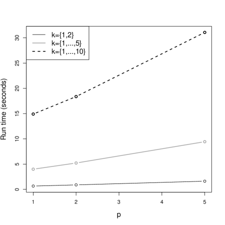
Figure S8. Median run time (seconds) to compute $P(\mathcal{M}_{k}\mid{\bf y})$ for all $k=1,\ldots,K$ via the ECP estimator (function bfnormmmix in R package mombf). Data was generated from a one-component standard multivariate Normal

We conducted further experiments to assess the computational scalability of the ECP estimator as a function of $n$, $p$ and the upper bound $K$ on the number of clusters. We simulated data for $n\in\{200,1000\}$, $p\in\{1,2,5\}$ and $K=\{2,5,10\}$ under a single-component multivariate Normal with zero mean and identity covariance matrix. Figure S8 shows the median run times. The time increased linearly with $n$ and slightly supra-linearly in $k$ and $p$. It is easy to show that the per-iteration computational complexity of the Gibbs sampler is linear in $n$, whereas to sample the covariance matrix (via a Cholesky decomposition) it is cubic in $p$. Regarding $k$ the Gibbs per-iteration complexity under a Normal-IWishart prior grows linearly with $k$ (hence so does obtaining ECP-based posterior model probabilities), however the post-processing step in (3.1) to evaluate the MOM-IW penalty contains $k(k-1)/2$ terms. Despite such supra-linear complexity our results show that for moderately large $(k,p)$ computations remain feasible. We reported total times for $k=1,\ldots,K$; one could use parallel computing or stop at the smallest $k$ such that $P(\mathcal{M}_{k}\mid{\bf y})<P(\mathcal{M}_{k-1}\mid{\bf y})$ which typically happens well before reaching $K$ (Chambaz and Rousseau, 2008).

4.2. Inference under a misspecified model

In practice the data-generating density may present non-negligible departures from the assumed class. An important case we investigate here is the presence of heavy tails, which under an assumed Normal mixture likelihood may affect both the chosen $k$ and the parameter estimates. We generated $n=600$ observations from $k^{*}=3$ bivariate T components with $4$ degrees of freedom, means $\bm{\mu}_{1}=(-1,1)^{\prime}$, $\bm{\mu}_{2}=-\bm{\mu}_{1}$, $\bm{\mu}_{3}=(6,6)^{\prime}$, a common scale matrix with elements $\sigma_{11}=\sigma_{22}=2$ and $\sigma_{12}=\sigma_{21}=-1$ and $\eta_{1}=\eta_{2}=\eta_{3}=1/3$. We considered up to $K=6$ components with either homogeneous $\Sigma_{1}=\ldots=\Sigma_{k}$ or heterogeneous covariances, giving a total of 11 models.

Table S4 summarises the results. BIC and sBIC strongly favoured $\hat{k}=4$ components with unequal covariances, AIC chose $\hat{k}=6$ components with unequal covariances, and the Normal-IW prior placed most posterior probability on $k\in\{5,6\}$ with common covariances. In contrast, our MOM-IW assigned posterior probability 1 (up to rounding) to $k=3$ with equal covariances. To provide further insight Figure 4 shows the component contours for $\hat{k}$ under each method, estimating $\hat{\bm{\vartheta}}_{\hat{k}}$ via maximum likelihood (AIC, BIC, sBIC) or posterior modes (Normal-IW, MOM-IW). The means of the three MOM-IW components matched those of the true T components. The BIC and sBIC approximated the two mildly-separated components with two normals centered roughly at (0,0), whereas the AIC split the components even further. The two extra components in the Normal-IW solution essentially account for heavy tails. This example illustrates how by penalizing poorly-separated or low-weight components NLPs may induce a form of robustness to model misspecification, although we remark that this is a finite-sample effect and would eventually vanish as $n\rightarrow\infty$.

BIC/sBIC	AIC
Normal-IW	MOM-IW

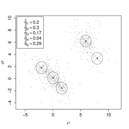
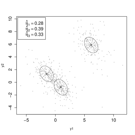
Figure 4. Misspecified model. Estimated contours for BIC and sBIC (top left), AIC (top right), Normal-IW (bottom left) and MOM-IW (bottom right). Points indicate the simulated data.

4.3. Cytometry data

We analysed the Graf-versus-Host flow cytometry data in Brinkman et al. (2007), an experiment used for cell counting, e.g. to diagnose diseases. The data contain $p=4$ variables called CD3, CD4, CD8b and CD8. The study goal was to find cell subpopulations with positive CD3, CD4 and CD8b (CD3+/CD4+/CD8b+), i.e. high values in the first three variables. Interestingly, the authors created a control sample designed not to contain any CD4+/CD8b+ cells. Following the analysis in Baudry et al. (2012), we selected the $n=1,126$ cells in the control sample for which CD3 $>280$.

BIC	AIC/sBIC
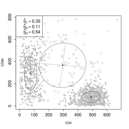
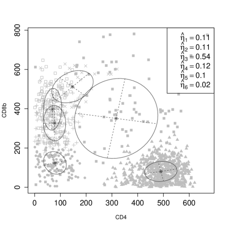
Normal-IW	MOM-IW

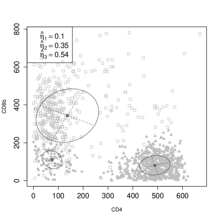
Figure 5. Projection of the variables CD4 and CD8b for the Cytometry data-set, classification of observations and contours using EM algorithm for BIC and AIC/sBIC (top), and under Normal-IW and MOM-IW (bottom).

Figure 5 plots (CD4,CD8b) values and the solution chosen by BIC, AIC, sBIC, Normal-IW and MOM-IW. The first four methods identified a CD4+/CD8b+ subpopulation that, as discussed, is not there by design, whereas it was not present in the MOM-IW solution. Intuitively, the spurious CD4+/CD8b+ cluster contains a few outlying observations, and our MOM-IW penalises such a low-weight component. These results illustrate the benefits of jointly penalising small weights and overlapping components. See Table S5 for further details, e.g. the Normal-IW and MOM-IW chose $k=3$ with 0.928 and 0.995 posterior probability, respectively.

4.4. Old Faithful

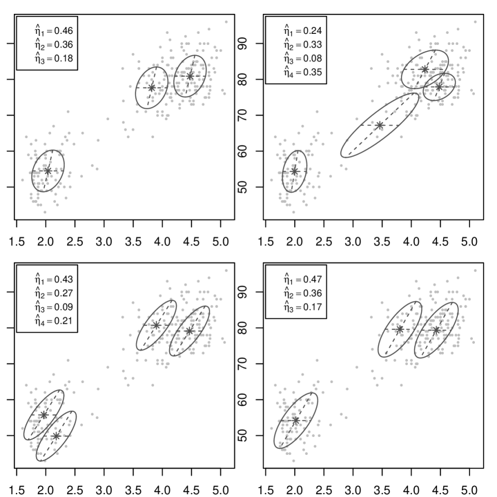
Figure S14. Faithful dataset. The x-axis portrays the eruption time (minutes) and the y-axis the waiting time until the next eruption (minutes). Contours for the model chosen by BIC/sBIC and AIC (top), Normal-IW and MOM-IW (bottom), from left to right and the points indicate the data.

We briefly describe this classical example to illustrate potential issues with poorly-separated components. The results are in Table S6 and Figure S14. The Old Faithful is a cone-type geyser in the Yellowstone National Park. We seek clusters in a dataset with $n=272$ eruptions recording their duration and the time to the next eruption (dataset faithful in R). We considered up to $K=6$ Normal components either with equal or unequal covariance matrices. Our MOM-IW selected $k=3$ equal-covariance components with 0.967 posterior probability. The Normal-IW chose $k=4$ with 0.473 posterior probability, this resulted from splitting an MOM-IW component in the lower-left corner into two. The sBIC and BIC chose $\hat{k}=3$ components with roughly the similar location as the MOM-IW, though their shapes were slightly different, whereas AIC returned $\hat{k}=4$.

4.5. Fisher’s Iris data

We present another classical dataset by Fisher (1936) for the practical reason that there is a ground truth for the underlying number of subpopulations. The data contain four variables ($p=4$) measuring the dimensions of $n=150$ iris flowers. The plants are known to belong to $k^{*}=3$ species, setosa, versicolor and virginica, each with 50 observations. We compare the ability of the various methods to recover these three species in an unsupervised fashion. We considered up to $K=6$ Normal components with either equal or unequal covariances.

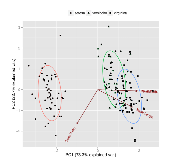
Figure S15. Principal components for the Fisher’s Iris data-set, classification of observations and contours using EM algorithm under MOM-IW.

Table S7 provides posterior model probabilities. The BIC and sBIC supported $\hat{k}=2$ and $\hat{k}=4$ components with unequal covariances, respectively. Upon inspection the BIC solution merged the versicolor and virginica species into a single component, akin to its lack of sensitivity observed in Section 4.1, whereas the sBIC split the versicolor species into two components. The AIC supported $\hat{k}=6$ with unequal covariances. Both the Normal-IW and our MOM-IW chose $\hat{k}=3$, but the evidence under the former was weaker ($P^{L}(\mathcal{M}_{3}\mid{\bf y})=0.81$ and $P(\mathcal{M}_{3}\mid{\bf y})=1$ respectively). Figure S15 shows the MOM-IW solution contours for the first two principal components (accounting for 96.0% of the variance), which closely resemble the three species.

4.6. Comparison to overfitted mixtures

Table 2 and Table S8 summarise the results from analysing the datasets from Sections 4.2-4.5 with overfitted mixtures and repulsive overfitted mixtures (respectively). Here repulsion was induced by a pMOM penalty where $g$ is set to its default in Section 2.3. We set $k=6$ and report the posterior distribution of the number of empty components (with no assigned observations) from the MCMC output. Note that $k=6$ implies overfitted mixtures as our analyses in Sections 4.2-4.5 suggested less than 6 components. To assess sensitivity we tested prior parameter values $q=1$ (no shrinkage), $q=0.01$ (satisfying Rousseau and Mengersen (2011) and Gelman et al. (2013)) and $3\times 10^{-8}$ (proposed by Havre et al. (2015)). We observed little differences between overfitted and repulsive overfitted mixtures. As expected, in general smaller $q$ led to less occupied components in the posterior, except in the cytometry data where the posterior focused on 6 components for all $q$. Note that $q=3\times 10^{-8}$ recovered the true $k^{*}=3$ in the misspecified example from Section 4.2, whereas this was not the case in the Iris and Cytometry data that truly contain 3 subpopulations. The results for the faithful data matched those of the MOM-IW.

Table 2. Posterior distribution on the number of non-empty components $m=\sum_{j=1}^{k}\mbox{I}(n_{j}>0)$ in overfitted mixtures with common $\Sigma_{j}=\Sigma$. The Misspecified, Faithful, Iris and Cytometry data.

	$\hat{P}(m\mid{\bf y},\mathcal{M}_{6})$
	$m=1$	$m=2$	$m=3$	$m=4$	$m=5$	$m=6$
			$q=1$
Misspecified	0.00	0.00	0.00	0.00	0.07	0.93
Faithful	0.00	0.00	0.00	0.01	0.15	0.85
Fisher’s Iris	0.00	0.99	0.01	0.00	0.00	0.00
Cytometry	0.00	0.00	0.00	0.00	0.00	1.00
			$q=0.01$
Misspecified	0.00	0.00	0.03	0.35	0.56	0.06
Faithful	0.00	0.00	0.63	0.31	0.04	0.02
Fisher’s Iris	0.00	1.00	0.00	0.00	0.00	0.00
Cytometry	0.00	0.00	0.00	0.00	0.00	1.00
			$q=3.10^{-8}$
Misspecified	0.00	0.00	0.95	0.00	0.00	0.05
Faithful	0.00	0.00	0.96	0.00	0.01	0.03
Fisher’s Iris	0.00	1.00	0.00	0.00	0.00	0.00
Cytometry	0.00	0.00	0.00	0.00	0.00	1.00

4.7. Simulation with Binomial mixtures

To assess the performance of MOM-Beta (default $a=1/2$, $g=7.11$) and Beta(1,1) priors as well as the BIC and sBIC, we reproduced the Binomial mixture example used by Drton and Plummer (2017) to illustrate the sBIC. We generated 200 data sets of sample sizes $n=50$, 200 and 500 from a $k^{*}=4$ component Binomial mixture with $L_{if}=30$ trials for all $i=1,\ldots,n$, equal component weights $\eta_{j}=1/4$ and component-specific success probabilities $\theta_{j}=j/5$ for $j=1,\ldots,4$. We computed the two sBIC versions $\overline{\text{sBIC}}$ and $\overline{\text{sBIC}}_{05}$.

Figure 6 shows the results. The two sBIC versions ameliorated the BIC’s overpenalization as reported in Drton and Plummer (2017), whereas the Beta prior often returned too many components. The proportion of correct model selections was generally highest for the MOM-Beta, particularly for smaller $n$ (roughly 50% of the simulations when $n=50$, relative to 25% for $\overline{\text{sBIC}}_{05}$). To assess sensitivity Figure S3 shows the results for alternative prior parameter settings $g=16.09$ and $g=29.99$ discussed in Supplementary Section S6. These larger $g$ values result in more informative priors that adversely affect inference, reinforcing our recommendation for $g=7.11$.

n=50

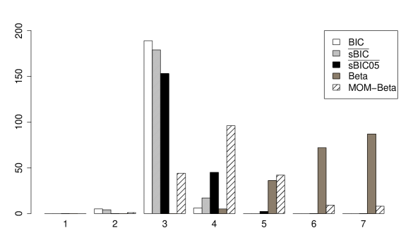
n=200

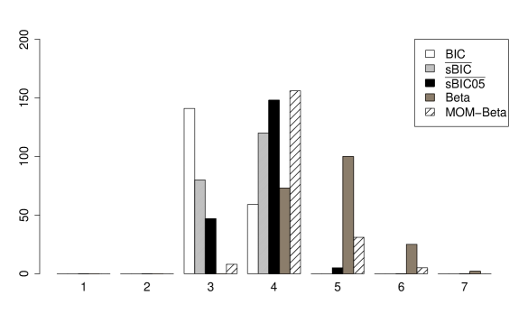
n=500

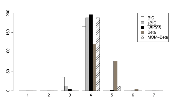
Figure 6. Binomial mixture. Frequencies of $\hat{k}$ for BIC, $\overline{\text{sBIC}}$, $\overline{\text{sBIC}}_{05}$, Beta and MOM-Beta. Results from 200 data sets with $n=50$, 200 and 500, $L=30$ and $k^{*}=4$

4.8. Political blog data

We illustrate product Binomial mixtures using a dataset on $n=773$ USA political blogs from 2008 (Chang, 2015). Each blog provides word counts (how many times a given word was used). To facilitate interpretation we combined similar words (e.g. america, american and americans, see Table S9) and selected the $p=234$ words with overall frequency above 100. We fitted a product Binomial mixture $y_{if}\mid z_{i}=j,\theta_{jf}\sim\text{Bin}(\theta_{jf},L_{i})$, where $L_{i}$ is the total number of words in blog $i=1,...,773$. We considered MOM-Beta and Beta priors, the BIC and AIC. The MOM-Beta parameters were set to the default $(a,g)=(0.5,2)$ whereas as a local prior we chose the Beta$(1,1)$ (Section 2.3).

BIC	AIC
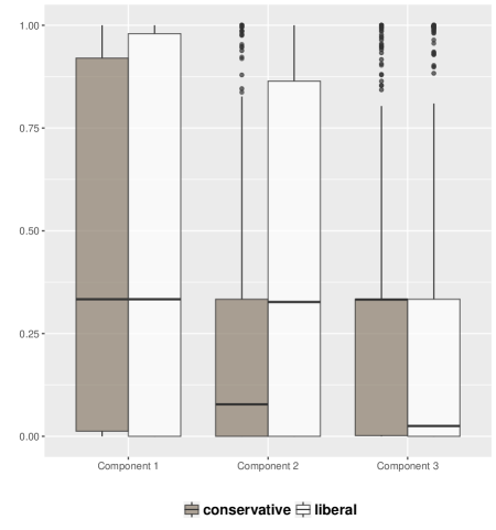
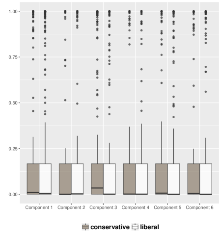
Beta	MOM-Beta

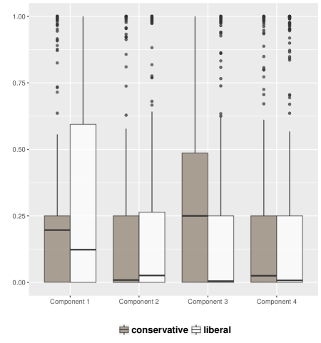
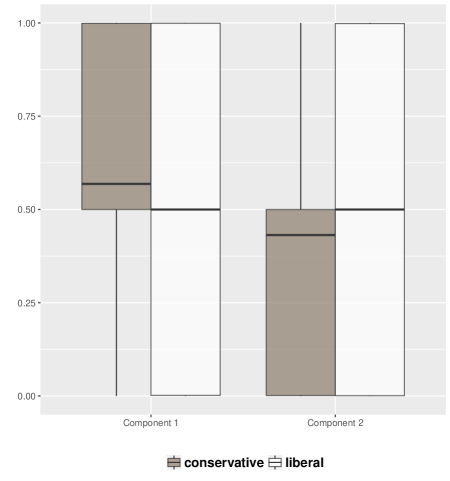
Figure S16. Estimated cluster probabilities $p(z_{i}=j|{\bf y},\mathcal{M}_{j})$ under BIC, AIC, Beta and MOM-Beta for documents labelled as conservative or liberal

The MOM-Beta and Beta selected $\hat{k}=2$ and $\hat{k}=4$ both with posterior probability one (up to rounding), whereas BIC and AIC chose $\hat{k}=3$ and $\hat{k}=6$ respectively (Table S10). To assess the inferred components, these data contain an independent labeling that classifies blogs either as liberal or conservative. Figure S16 displays the estimated cluster probabilities (Algorithm S5) for liberal and conservative blogs. Interestingly under the MOM-Beta prior conservative blogs fell mostly in Component 1. Figure 7 shows the most characteristic words for each MOM-Beta component ($\chi^{2}$ residual$>2$ when cross-tabulating word count versus assigned component). For instance, “war, iraq, tax, government” are representative of Component 1 whereas “polls, votes, percent, delegates” are representative of Component 2. In contrast, under the Beta prior Components 2 and 4 showed a similar distribution for liberal and conservative blogs and the clusters returned by the AIC did not show appreciable differences between conservative or liberal blogs.

Component 1	Component 2

Figure 7. Political blog data. Each word was assigned to its most probable component under a MOM-Beta prior. Word sizes based on $\chi^{2}$ residuals from cross-tabulating word frequency versus assigned component

5. Conclusions

The use of NLPs for selecting mixture components leads to solutions that balance parsimony and sensitivity, and also facilitates interpretation in terms of well-separated subpopulations. From a theoretical standpoint the formulation asymptotically enforces parsimony under the wide class of generically identifiable mixtures, which we confirmed in finite $n$ examples. As another practical issue defining prior dispersion is often regarded as an inconvenience, here we showed how it can be advantageously calibrated to detect well-separated components resulting in multimodality. We also showed that the computations required to implement NLPs are comparable to those for standard local priors and, although not exploited here, they can easily be parallelized for multiple $k$. In particular the ECP estimator provides a convenient strategy to estimate posterior model probabilities for non-local and local priors, by utilizing readily available MCMC output.

Our examples showed that BIC may pathologically miss components, in some instances even with large $n$. The AIC and local priors tended to add spurious components in simulations and in datasets with known subgroup structure. The sBIC showed a mixed behavior that was similar to the BIC in some instances and to local priors or the AIC in others. Overfitted and repulsive overfitted mixtures proved useful in several examples, but prior parameters and the choice of $k$ need to be carefully calibrated. Our framework can also be sensitive to prior specification, but as we illustrated there are natural defaults based on multi-modality and minimal informativeness that result in competitive behaviour. Despite the resemblance between NLPs and repulsive overfitted mixtures we emphasise that the former require not only a repulsive force but also penalising low-weight components, and that this was found to improve inference in our examples. A related intriguing observation was that, by penalizing poorly-separated and low-weight components, NLPs showed robustness to model misspecification in an example. It would be interesting to study the combined effect of NLPs and robust likelihoods.

Supplementary material

S1. Conditions A1-A4 in Rousseau and Mengersen [2011]

For convenience we reproduce verbatim Conditions A1-A4 in Rousseau and Mengersen [2011], adjusted to the notation we used in this paper. Their Condition A5 is trivially satisfied by our $\bm{\eta}\sim\mbox{Dir}(q)$ prior, hence is not reproduced here. Recall that we defined $p_{k^{*}}^{*}({\bf y})=p({\bf y}\mid\bm{\vartheta}_{k^{*}}^{*},\mathcal{M}_{k^{*}})$ to be the data-generating truth.

We denote $\Theta_{k}^{*}=\{\bm{\vartheta}_{k}\in\Theta_{k};p({\bf y}\mid\bm{\vartheta}_{k},\mathcal{M}_{k})=p_{k^{*}}^{*}({\bf y})\}$ and let $\log(p({\bf y}\mid\bm{\vartheta}_{k},\mathcal{M}_{k}))$ be the log-likelihood calculated at $\bm{\vartheta}_{k}$. Denote $F_{0}(g)=\int p({\bf y}\mid\bm{\vartheta}_{k^{*}}^{*},\mathcal{M}_{k^{*}})g({\bf y})d{\bf y}$ where $g(\cdot)$ is a probability density function, denote by $\text{Leb}(A)$ the Lebesgue measure of a set $A$ and let $\nabla p({\bf y}\mid\bm{\theta})$ be the vector of derivatives of $p({\bf y}\mid\bm{\theta})$ with respect to $\bm{\theta}$, and $\nabla^{2}p({\bf y}\mid\bm{\theta})$ be the second derivatives with respect to $\bm{\theta}$. Define for $\epsilon\geq 0$

$$\bar{p}({\bf y}\mid\bm{\theta}) =\sup_{|\bm{\theta}^{l}-\bm{\theta}|\leq\epsilon}p({\bf y}\mid\bm{\theta}^{l}), \underline{p}({\bf y}\mid\bm{\theta}) =\inf_{|\bm{\theta}^{l}-\bm{\theta}|\leq\epsilon}p({\bf y}\mid\bm{\theta}^{l})$$

We now introduce some notation that is useful to characterize $\Theta_{k}^{*}$, following Rousseau and Mengersen [2011]. Let ${\bf w}=(w_{i})_{i=0}^{k^{*}}$ with $0=w_{0}<w_{1}<...<w_{k^{*}}\leq k$ be a partition of $\{1,...,k\}$. For all $\bm{\vartheta}_{k}\in\Theta_{k}$ such that $p({\bf y}\mid\bm{\vartheta}_{k},\mathcal{M}_{k})=p_{k}^{*}({\bf y})$ there exists ${\bf w}$ as defined above such that, up to a permutation of the labels,

$$\forall i=1,...,k^{*},\;\;\;\bm{\theta}_{w_{i-1}+1}=...=\bm{\theta}_{w_{i}}=\bm{\theta}_{i}^{*},\;\;\;\eta(i)=\sum_{j=w_{i-1}+1}^{w_{i}}\eta_{j}=\eta_{i}^{*},\;\;\;\eta_{w_{k^{*}+1}}=...=\eta_{k}=0.$$

In other words, $I_{i}=\{w_{i-1}+1,...,w_{i}\}$ represents the cluster of components in $\{1,...,k\}$ having the same parameter as $\bm{\theta}_{i}^{*}$. Then define the following parameterisation of $\bm{\vartheta}_{k}\in\Theta_{k}$ (up to permutation)

$$\bm{\iota_{w}} =\left((\bm{\theta}_{j})_{j=1}^{w_{k^{*}}},(r_{i})_{i=1}^{k^{*}-1},(\eta_{j})_{j=w_{k^{*}+1}}^{k}\right)\in\mathbb{R}^{pw_{k^{*}}+k^{*}+k-w_{k^{*}}-1}, r_{i} =\eta(i)-\eta_{i}^{*}, i =1,...,k^{*},$$

and

$$\bm{\varpi_{w}} =\left((f_{j})_{j=1}^{w_{k^{*}}},\bm{\theta}_{w_{k^{*}}+1},...,\bm{\theta}_{{k}}\right), f_{j} =\dfrac{\eta_{j}}{\eta(i)},\;\;\;\text{when}\;\;\;j\in I_{i}=\{w_{i-1}+1,...,w_{i}\},$$

note that for $p({\bf y}\mid\bm{\vartheta}_{k^{*}}^{*},\mathcal{M}_{k^{*}})$

$$\bm{\iota_{w}}^{*}=(\bm{\theta}_{1}^{*},...,\bm{\theta}_{1}^{*},\bm{\theta}_{2}^{*},...,\bm{\theta}_{2}^{*},...,\bm{\theta}_{k^{*}}^{*},...,\bm{\theta}_{k^{*}}^{*},0...0...0)$$

where $\bm{\theta}_{i}^{*}$ is repeated $w_{i}-w_{i-1}$ times in the above vector for any $\bm{\varpi_{w}}$. Then we parameterize $(\bm{\iota_{w}},\bm{\varpi_{w}})$, so that $p({\bf y}\mid\bm{\vartheta}_{k},\mathcal{M}_{k})=p({\bf y}\mid(\bm{\iota_{w}},\bm{\varpi_{w}}),\mathcal{M}_{k})$ and we denote

$\nabla p({\bf y}\mid(\bm{\iota_{w}^{*}},\bm{\varpi_{w}}),\mathcal{M}_{k})$ and $\nabla^{2}p({\bf y}\mid(\bm{\iota_{w}^{*}},\bm{\varpi_{w}}),\mathcal{M}_{k})$ the first and second derivatives of $p({\bf y}\mid(\bm{\iota_{w}},\bm{\varpi_{w}}),\mathcal{M}_{k})$ with respect to $\bm{\iota_{w}}$ and computed at $\bm{\vartheta}_{k^{*}}^{*}=(\bm{\iota_{w}^{*}},\bm{\varpi_{w}})$. We also denote by $P^{L}(\cdot\mid{\bf y},\mathcal{M}_{k})$ the posterior distribution using a LP.

Conditions

1. $L_{1}$ consistency. For all $\epsilon=(\log n)^{e}/\sqrt{n}$ with $e\geq 0$ as $n\rightarrow\infty$

   $$P^{L}\left(\int\left|p({\bf z}\mid\bm{\vartheta}_{k},\mathcal{M}_{k})-p_{k}^{*}({\bf z})\right|d{\bf z}>\epsilon\mid{\bf y},\mathcal{M}_{k}\right)\rightarrow 0$$

   in probability with respect to $p({\bf y}\mid\bm{\vartheta}_{k^{*}}^{*},\mathcal{M}_{k^{*}})$.

2. Regularity. The component density $p({\bf y}\mid\bm{\theta})$ indexed by a parameter $\bm{\theta}\in\Theta$ is three times differentiable and regular in the sense that for all $\bm{\theta}\in\Theta$ the Fisher information matrix associated with $p({\bf y}\mid\bm{\theta})$ is positive definite at $\bm{\theta}$. Denote $\nabla^{3}p({\bf y}\mid\bm{\theta})$ the array whose components are

   $$\frac{\partial^{3}p({\bf y}\mid\bm{\theta})}{\partial_{\bm{\theta}_{i1}}\partial_{\bm{\theta}_{i2}}\partial_{\bm{\theta}_{i3}}}$$

   For all $i\leq k^{*}$, there exists $\epsilon>0$ such that

   $$F_{0} \left(\dfrac{\bar{p}({\bf y}\mid\bm{\theta}_{i}^{*})^{3}}{\underline{p}({\bf y}\mid\bm{\theta}_{i}^{*})^{3}}\right)<\infty, F_{0} \left(\dfrac{\sup_{|\bm{\theta}-\bm{\theta}^{*}|\leq\epsilon}|\nabla p({\bf y}|\bm{\theta})|^{3}}{\underline{p}({\bf y}\mid\bm{\theta}_{i}^{*})^{3}}\right)<\infty, F_{0} \left(\frac{|p({\bf y}|\bm{\theta}_{i}^{*})|^{4}}{(p({\bf y}\mid\bm{\vartheta}_{k^{*}}^{*},\mathcal{M}_{k^{*}}))^{4}}\right)<\infty,$$

   $$F_{0} \left(\dfrac{\sup_{|\bm{\theta}-\bm{\theta}^{*}|\leq\epsilon}|\nabla^{2}p({\bf y}\mid\bm{\theta})|^{2}}{\underline{p}({\bf y}\mid\bm{\theta}_{i}^{*})^{2}}\right)<\infty, F_{0} \left(\dfrac{\sup_{|\bm{\theta}-\bm{\theta}^{*}|\leq\epsilon}|\nabla^{3}p({\bf y}\mid\bm{\theta})|^{2}}{\underline{p}({\bf y}\mid\bm{\theta}_{i}^{*})}\right)<\infty.$$

   Assume also that for all $i=1,...,k^{*}$, $\bm{\theta}_{i}^{*}\in\text{int}(\Theta^{k})$ the interior of $\Theta^{k}$.

3. Integrability. There exists $\Theta^{k^{*}}\subset\Theta^{k}$ satisfying $\text{Leb}(\Theta^{k^{*}})>0$ and for all $i\leq k^{*}$

   $$d(\bm{\theta}_{i}^{*},\Theta^{k^{*}})=\inf_{\bm{\theta}\in\Theta^{k^{*}}}|\bm{\theta}-\bm{\theta}_{i}^{*}|>0$$

   and such that for all $\bm{\theta}\in\Theta^{k^{*}}$,

   $$F_{0} \left(\dfrac{p({\bf y}\mid\bm{\theta})^{4}}{(p({\bf y}\mid\bm{\vartheta}_{k^{*}}^{*},\mathcal{M}_{k^{*}}))^{4}}\right)<\infty, F_{0} \left(\dfrac{p({\bf y}\mid\bm{\theta})^{3}}{\underline{p}({\bf y}\mid\bm{\theta}_{i}^{*})^{3}}\right)<\infty, \forall i\leq k^{*}.$$

4. Stronger identifiability.

   For all ${\bf w}$ partitions of $\{1,...,k\}$ as defined above, let $\bm{\vartheta}_{k}\in\Theta_{k}$ and write $\bm{\vartheta}_{k}$ as $(\bm{\iota_{w}},\bm{\varpi_{w}})$; then

   $$(\bm{\iota_{w}}-\bm{\iota_{w}}^{*})^{{}^{\prime}}\nabla p({\bf y}\mid(\bm{\iota_{w}^{*}},\bm{\varpi_{w}}),\mathcal{M}_{k})+\dfrac{1}{2}(\bm{\iota_{w}}-\bm{\iota_{w}}^{*})^{{}^{\prime}}\nabla^{2}p({\bf y}\mid(\bm{\iota_{w}^{*}},\bm{\varpi_{w}}),\mathcal{M}_{k})(\bm{\iota_{w}}-\bm{\iota_{w}}^{*})=0\Leftrightarrow$$

   $$\forall i\leq k^{*},r_{i}=0\;\;\text{and}\;\;\forall j\in I_{i}\;\;f_{j}(\bm{\theta}_{j}-\bm{\theta}_{j}^{*})=0,\;\;\forall i\geq w_{k^{*}}+1,\;\;p_{i}=0.$$

Assuming also that if $\bm{\theta}\notin\{\bm{\theta}_{1},...,\bm{\theta}_{k}\}$ then for all functions $h_{\bm{\theta}}$ which are linear combinations of derivatives of $p({\bf y}\mid\bm{\theta})$ of order less than or equal to 2 with respect to $\bm{\theta}$, and all functions $h_{1}$ which are also linear combinations of derivatives of the $p({\bf y}\mid\bm{\theta}_{j})$’s $j=1,2,..,k$ and its derivatives of order less or equal to 2, then $\alpha h_{\bm{\theta}}+\beta h_{1}=0$ if and only if $\alpha h_{\bm{\theta}}=\beta h_{1}=0$.

Extension to non compact spaces: If $\subset\Theta^{k}$ is not compact then we also assume that for all sequences $\bm{\theta}_{n}$ converging to a point in $\partial\Theta^{k}$ the frontier of $\Theta^{k}$, considered as a subset of $\Re\cup\left\{-\infty,\infty\right\}^{p}$, $p({\bf y}\mid\bm{\theta}_{n})$ converges pointwise either to a degenerate function or to a proper density $p(\cdot)$ such that $p(\cdot)$ is linearly independent of any null combinations of $p^{*}({\bf y}\mid\bm{\theta}_{i})$, $\nabla p^{*}({\bf y}\mid\bm{\theta}_{i})$ and $\nabla^{2}p^{*}({\bf y}\mid\bm{\theta}_{i})$, $i=1,...,k^{*}$.

S2. Prior normalization constant for MOM priors

Lemma 1.

Let $p(\bm{\zeta}\mid\mathcal{M}_{k})$ be as in (2.7). Then

$$C_{k}=\sum_{s\in S_{k}}\left(\prod_{l=1}^{pk}\kappa_{s}\right)\sum_{v(1,2)=0}^{1}\ldots\sum_{v(k-1,k)=0}^{1}(-1)^{\sum_{i<j}v(i,j)}\left(\prod_{l=1}^{pk}\prod_{m=1}^{pk}\frac{b_{lm}^{s_{l,m}}(v)}{s_{l,m}!}\right)$$

where $\kappa_{s}=E^{L}(\theta_{11}^{\sum_{m=1}^{pk}s_{lm}+s_{ml}})$, $S_{k}=\left\{(s_{1,1},s_{1,2},\ldots,s_{pk,pk}):\sum_{l=1}^{pk}\sum_{m=1}^{pk}s_{l,m}=k(k-1)/2\right\}$ with non-negative integers $0\leq s_{l,m}\leq k(k-1)/2$, and $b_{lm}(v)$ is the $(l,m)$ element of the $pk\times pk$ matrix $B_{v}$ given by

$$\begin{cases}b_{ll}=\frac{1}{2}(k-1)-\sum_{i<j}v(i,j)\mbox{, }l=1+p(i-1),\ldots,pi\\ b_{lm}=b_{ml}=-\frac{1}{2}+\sum_{i<j}v(i,j)\mbox{, }(1+p(i-1),1+p(j-1)),\ldots,(pi,pj)\end{cases}.$$

We remark that Lemma 1 holds for any $p^{L}(\bm{\zeta})$ composed by independent and identically-distributed $p^{L}(\zeta_{jf})$ and that $\kappa_{s}$ requires raw moments up to order $k(k-1)/2$, which can be pre-computed. Specifically, for the MOM-Beta prior in (2.6)

$$\kappa_{s}=\left(\frac{\Gamma(g)}{\Gamma(ag)}\right)^{pk}\frac{\Gamma\left(ag+\sum_{m=1}^{pk}s_{lm}+s_{ml}\right)}{\Gamma\left(g+\sum_{m=1}^{pk}s_{lm}+s_{ml}\right)}.$$

For certain common settings with MOM-IW and MOM-Beta priors, Lemma 1 can be simplified, see Corollaries 1-3.

		$\mbox{Var}(\theta_{jf}-\theta_{j^{\prime}f}\mid\mathcal{M}_{2})$
$p$	Default $g$	Default $g$	$g=2$
1	7.11	1/6	0.400
2	4.39	1/6	0.283
3	3.54	1/6	0.244
4	3.13	1/6	0.225
5	2.89	1/6	0.213
6	2.74	1/6	0.206
7	2.63	1/6	0.200
8	2.55	1/6	0.196
9	2.48	1/6	0.193
10	2.43	1/6	0.190
11	2.39	1/6	0.188
12	2.36	1/6	0.186
13	2.33	1/6	0.185
14	2.31	1/6	0.183
15	2.29	1/6	0.182
16	2.27	1/6	0.181
17	2.25	1/6	0.180
18	2.24	1/6	0.180
19	2.23	1/6	0.179
20	2.21	1/6	0.178

Table S1. Default $g$ in MOM-Beta$(0.5g,0.5g)$ prior giving $\mbox{Var}(\theta_{jf}-\theta_{j^{\prime}f}\mid\mathcal{M}_{2})=1/6$ as a function of $p$, and variance for $g=2$. For $p>20$ we recommend the default $g=2$

S3. Prior variance under MOM-Beta priors

Let $p(\bm{\theta}\mid\mathcal{M}_{k})$ be the MOM-Beta prior in (2.6) and $p^{L}(\bm{\theta}\mid\mathcal{M}_{k})$ be the Beta prior in (2.9) with parameters $(a_{L},g_{L})=(0.5,2)$. Our suggested defaults are setting $a=0.5$ and $g$ (2.6) such that

$$\mbox{Var}_{p}(\theta_{jf}-\theta_{j^{\prime}f}\mid\mathcal{M}_{k})=\mbox{Var}_{p^{L}}(\theta_{jf}-\theta_{jf^{\prime}}\mid\mathcal{M}_{k})=\frac{1}{6}.$$

It is in principle possible to find such $g$ by noting that, due to $(\theta_{jf},\theta_{jf^{\prime}})$ being exchangeable a priori we have $E_{p}(\theta_{jf}-\theta_{j^{\prime}f}\mid\mathcal{M}_{k})=0$. Hence $\mbox{Var}_{p}(\theta_{jf}-\theta_{j^{\prime}f}\mid\mathcal{M}_{k})=$

$$\int\frac{(\theta_{jf}-\theta_{j^{\prime}f})^{2}}{C_{k}}\prod_{1\leq i<j\leq k}\sum_{f}(\theta_{if}-\theta_{jf})^{2}\prod_{j=1}^{k}\prod_{f=1}^{p}\text{Beta}(\theta_{jf};ag,(1-a)g)d\bm{\theta}$$

and one may expand the product within the integral as a sum involving products of polynomials. As illustration for $p=1$ and $a=0.5$ simple algebra shows

$$\mbox{Var}_{p}(\theta_{j1}-\theta_{j^{\prime}1}\mid\mathcal{M}_{2})=1.5\frac{2+g}{(1+g)(3+g)}$$

$$\mbox{Var}_{p}(\theta_{j1}-\theta_{j^{\prime}1}\mid\mathcal{M}_{3})=2\frac{4+g}{(3+g)(5+g)}$$

and so on for larger $k$. For instance if $k=2$ then the desired defaults are $(a,g)=(0.5,7.11)$, and for $k=3$ they would be $(a,g)=(0.5,8.08)$. This strategy grows tedious for larger $k$ as the expressions become less manageable and even evaluating $C_{k}$ becomes non-trivial for general $p$.

We adopt the simpler alternative strategy of focusing on the $k=2$ case, this is analogous to the approach to set the MOM-Normal prior dispersion in continuous mixtures and in practice we observed that the target prior variance becomes more robust to $g$ as $k$ grows (Figure S2). That is, our strategy is

$$\frac{1}{6}=\mbox{Var}_{p}(\theta_{jf}-\theta_{j^{\prime}f}\mid\mathcal{M}_{2})=2\left[E_{p}(\theta_{11}^{2}\mid\mathcal{M}_{2})-E_{p}(\theta_{11}\theta_{21}\mid\mathcal{M}_{2})\right],$$

where the right-hand side follows from exchangeability. We first state the result and subsequently outline its derivation.

$$E_{p}(\theta_{11}^{2}\mid\mathcal{M}_{2}) =\frac{ag+1}{2p(1-a)}\left[\frac{(ag+2)(ag+3)}{(g+2)(g+3)}+\frac{a(ag+1)+2(p-1)a(1-a)}{g+1}-\frac{2a(ag+2)}{g+2}\right]$$

$$E_{p}(\theta_{11}\theta_{21}\mid\mathcal{M}_{2}) =\frac{a}{p(1-a)}\left[\frac{(ag+1)(ag+2)}{g+2}-\frac{(ag+1)^{2}}{(g+1)}+(p-1)a(1-a)\right]$$

For the particular case $(a,g)=(0.5,2)$ one obtains

$$\mbox{Var}_{p}(\theta_{jf}-\theta_{j^{\prime}f}\mid\mathcal{M}_{2})=\frac{1}{p}\left(\frac{2}{5}+\frac{p-1}{6}\right),$$

which clearly converges to $1/6$ as $p\rightarrow\infty$. Table S1 lists the default $g$ giving $\mbox{Var}_{p}(\theta_{jf}-\theta_{j^{\prime}f}\mid\mathcal{M}_{2})=1/6$ for various $p$. For $p=20$ setting $g=2$ already gives $\mbox{Var}_{p}(\theta_{jf}-\theta_{j^{\prime}f}\mid\mathcal{M}_{2})=0.178$ and thus for $p>20$ we recommend $(a,g)=(0.5,2)$.

The remainder of this section outlines the derivation of $E_{p}(\theta_{11}^{2}\mid\mathcal{M}_{2})$ and $E_{p}(\theta_{11}\theta_{21}\mid\mathcal{M}_{2})$.

$$E_{p}(\theta_{11}^{2}\mid\mathcal{M}_{2})=\int\frac{\theta_{11}^{2}(\theta_{11}-\theta_{21})^{2}}{C_{2}}\prod_{j=1}^{2}\mbox{Beta}(\theta_{j1};ag,(1-a)g)d\theta_{j1}$$

$$+\int\frac{\theta_{11}^{2}}{C_{2}}\sum_{f=2}^{p}(\theta_{1f}-\theta_{2f})^{2}\prod_{j=1}^{2}\prod_{f=1}^{p}\mbox{Beta}(\theta_{jf};ag,(1-a)g)d\bm{\theta}$$

$$=\frac{a(ag+1)}{C_{2}(g+1)}\left[\frac{(ag+2)(ag+3)}{(g+2)(g+3)}+\frac{a(ag+1)}{g+1}-\frac{2a(ag+2)}{(g+2)}\right]-\frac{a(ag+1)\tilde{C}_{2}}{C_{2}(g+1)},$$

where the right-hand side follows from the moments of a Beta distribution and $\tilde{C}_{2}$ is the prior normalization constant for $p-1$ variables. Using that $C_{2}=2pa(1-a)/(g+1)$ and $\tilde{C}_{2}=2(p-1)a(1-a)/(g+1)$ gives the desired expression for $E_{p}(\theta_{11}^{2}\mid\mathcal{M}_{2})$. Similarly,

$$E_{p}(\theta_{11}\theta_{21}\mid\mathcal{M}_{2})=\int\frac{\theta_{11}\theta_{21}(\theta_{11}^{2}+\theta_{21}^{2}-2\theta_{11}\theta_{21})}{C_{2}}\prod_{j=1}^{2}\mbox{Beta}(\theta_{j1};ag,(1-a)g)d\theta_{j1}$$

$$+\int\frac{\theta_{11}\theta_{21}}{C_{2}}\sum_{f=2}^{p}(\theta_{1f}-\theta_{2f})^{2}\prod_{j=1}^{2}\prod_{f=1}^{p}\mbox{Beta}(\theta_{jf};ag,(1-a)g)d\theta_{jf}$$

$$\frac{2a^{2}(ag+1)}{C_{2}(g+1)}\left[\frac{ag+2}{g+2}-\frac{ag+1}{g+1}\right]-\frac{a^{2}\tilde{C}_{2}}{C_{2}}.$$

The result is obtained by plugging in $C_{2}=2pa(1-a)/(g+1)$, $\tilde{C}_{2}=2(p-1)a(1-a)/(g+1)$ and rearranging terms.

S4. Proofs

S4.1. Auxiliary lemmas to prove Theorem 1

We state and prove two auxiliary lemmas that will be used in the proof of Theorem 1.

Lemma 2.

Let $p(\bm{\vartheta}_{k}\mid\mathcal{M}_{k})=d_{\theta}(\bm{\theta})p^{L}(\bm{\theta}\mid\mathcal{M}_{k})p(\bm{\eta}\mid\mathcal{M}_{k})$ be the MOM prior in (2.4). Then $p(\bm{\vartheta}_{k}\mid\mathcal{M}_{k})=\tilde{d}_{\theta}(\bm{\theta})\tilde{p}^{L}(\bm{\theta}\mid\mathcal{M}_{k})p(\bm{\eta}\mid\mathcal{M}_{k})$, where $\tilde{d}_{\theta}(\bm{\theta})\leq c_{k}$ for some finite $c_{k}$,

$$\tilde{p}^{L}(\bm{\vartheta}_{k}\mid\mathcal{M}_{k})=\prod_{j=1}^{k}N\left(\bm{\mu}_{j};{\bf 0},(1+\epsilon)gA_{\Sigma}\right),$$

and $\epsilon\in(0,1)$ is an arbitrary constant.

Proof. The MOM prior has an unbounded penalty

$$d_{\theta}(\bm{\theta})=\frac{1}{C_{k}}\prod_{1\leq i<j\leq k}\left((\bm{\mu}_{i}-\bm{\mu}_{j})^{{}^{\prime}}A_{\Sigma}^{-1}(\bm{\mu}_{i}-\bm{\mu}_{j})/g\right)^{t},$$

however we may rewrite $d_{\theta}(\bm{\theta})p^{L}(\bm{\theta}\mid\mathcal{M}_{k})$

$$= d_{\theta}(\bm{\theta})\prod_{j=1}^{k}N\left(\bm{\mu}_{j};{\bf 0},gA_{\Sigma}\right)\dfrac{N\left(\bm{\mu}_{j};{\bf 0},(1+\epsilon)gA_{\Sigma}\right)}{N\left(\bm{\mu}_{j};{\bf 0},(1+\epsilon)gA_{\Sigma}\right)},$$

(S1) $$= \tilde{d}_{\theta}(\bm{\theta})\prod_{j=1}^{k}N\left(\bm{\mu}_{j};{\bf 0},(1+\epsilon)gA_{\Sigma}\right),$$

where $\epsilon\in(0,1)$ is an arbitrary constant and $\tilde{d}_{\theta}(\bm{\theta})=$

$$d_{\theta}(\bm{\theta})\prod_{j=1}^{k}\frac{N\left(\bm{\mu}_{j};{\bf 0},gA_{\Sigma}\right)}{N\left(\bm{\mu}_{j};{\bf 0},(1+\epsilon)gA_{\Sigma}\right)}=d_{\theta}(\bm{\theta})\prod_{j=1}^{k}(1+\epsilon)^{1/2}\exp\left\{-\dfrac{1}{2}\dfrac{\epsilon\bm{\mu}_{j}^{{}^{\prime}}A_{\Sigma}^{-1}\bm{\mu}_{j}}{(1+\epsilon)g}\right\}.$$

The fact that $\tilde{d}_{\theta}(\bm{\theta})$ is bounded follows from the fact that the product term is a Normal kernel and hence bounded, whereas $d_{\theta}(\bm{\theta})$ can only become unbounded when $\bm{\mu}_{j}A_{\Sigma}^{-1}\bm{\mu}_{j}\rightarrow\infty$ for some $j$, but this polynomial increase is countered by the exponential decrease in $\exp\left\{-\dfrac{1}{2}\dfrac{\epsilon\bm{\mu}_{j}^{{}^{\prime}}A_{\Sigma}^{-1}\bm{\mu}_{j}}{(1+\epsilon)g}\right\}$. ∎

Lemma 3.

Let $d_{\vartheta}(\bm{\vartheta}_{k})\in[0,c_{k}]$ be a bounded continuous function in $\bm{\vartheta}_{k}$, where $c_{k}$ is a finite constant. Let

$$g_{k}({\bf y})=E^{L}(d_{\vartheta}(\bm{\vartheta}_{k})\mid{\bf y},\mathcal{M}_{k})=\int d_{\vartheta}(\bm{\vartheta}_{k})p^{L}(\bm{\vartheta}_{k}\mid{\bf y},\mathcal{M}_{k})d\bm{\vartheta}_{k}.$$

If for any $\epsilon>0$ we have that $P^{L}(d_{\vartheta}(\bm{\vartheta})>\epsilon\mid{\bf y},\mathcal{M}_{k})\stackrel{{\scriptstyle P}}{{\longrightarrow}}0$ then $g_{k}({\bf y})\stackrel{{\scriptstyle P}}{{\longrightarrow}}0$. Alternatively, if there exists some $d_{k}^{*}>0$ such that for any $\epsilon>0$ $P^{L}(|d_{\vartheta}(\bm{\vartheta}_{k})-d_{k}^{*}|>\epsilon\mid{\bf y},\mathcal{M}_{k})\stackrel{{\scriptstyle P}}{{\longrightarrow}}1$, then $g_{k}({\bf y})\stackrel{{\scriptstyle P}}{{\longrightarrow}}d_{k}^{*}$.

Proof. Consider the case $P^{L}(d_{\vartheta}(\bm{\vartheta})>\epsilon\mid{\bf y},\mathcal{M}_{k})\stackrel{{\scriptstyle P}}{{\longrightarrow}}0$, then $g_{k}({\bf y})=$

$$\int_{d_{\vartheta}(\bm{\vartheta}_{k})<\epsilon}d_{\vartheta}(\bm{\vartheta}_{k})p^{L}(\bm{\vartheta}_{k}\mid{\bf y},\mathcal{M}_{k})d\bm{\vartheta}_{k}+\int_{d_{\vartheta}(\bm{\vartheta}_{k})>\epsilon}d_{\vartheta}(\bm{\vartheta}_{k})p^{L}(\bm{\vartheta}_{k}\mid{\bf y},\mathcal{M}_{k})d\bm{\vartheta}_{k}$$

$$\leq\epsilon P^{L}(d_{\vartheta}(\bm{\vartheta}_{k})<\epsilon\mid{\bf y},\mathcal{M}_{k})+c_{k}P^{L}(d_{\vartheta}(\bm{\vartheta}_{k})>\epsilon\mid{\bf y},\mathcal{M}_{k})$$

$$\leq\epsilon+c_{k}P^{L}(d_{\vartheta}(\bm{\vartheta}_{k})>\epsilon\mid{\bf y},\mathcal{M}_{k})\stackrel{{\scriptstyle P}}{{\longrightarrow}}\epsilon,$$

where $\epsilon>0$ is arbitrarily small. Hence $g_{k}({\bf y})\stackrel{{\scriptstyle P}}{{\longrightarrow}}0$.

Next consider the case $P^{L}(|d_{\vartheta}(\bm{\vartheta}_{k})-d_{k}^{*}|>\epsilon\mid{\bf y},\mathcal{M}_{k})\stackrel{{\scriptstyle P}}{{\longrightarrow}}1$. Then

$$g_{k}({\bf y}) >\int_{d_{\vartheta}(\bm{\vartheta}_{k})>d_{k}^{*}-\epsilon}d_{\vartheta}(\bm{\vartheta}_{k})p^{L}(\bm{\vartheta}_{k}\mid{\bf y})d\bm{\vartheta}_{k}$$

$$\geq(d_{k}^{*}-\epsilon)P^{L}\left(d_{\vartheta}(\bm{\vartheta}_{k})>d_{k}^{*}-\epsilon\mid{\bf y},\mathcal{M}_{k}\right)\stackrel{{\scriptstyle P}}{{\longrightarrow}}d_{k}^{*}-\epsilon,$$

and analogously $g_{k}({\bf y})=$

$$\int_{d_{\vartheta}(\bm{\vartheta}_{k})<d_{k}^{*}+\epsilon}d_{\vartheta}(\bm{\vartheta}_{k})p^{L}(\bm{\vartheta}_{k}\mid{\bf y},\mathcal{M}_{k})d\bm{\vartheta}_{k}+\int_{d_{\vartheta}(\bm{\vartheta}_{k})>d_{k}^{*}+\epsilon}d_{\vartheta}(\bm{\vartheta}_{k})p^{L}(\bm{\vartheta}_{k}\mid{\bf y},\mathcal{M}_{k})d\bm{\vartheta}_{k}$$

$$\leq(d_{k}^{*}+\epsilon)+c_{k}P^{L}(d_{\vartheta}(\bm{\vartheta}_{k})>d_{k}^{*}+\epsilon\mid{\bf y},\mathcal{M}_{k})\stackrel{{\scriptstyle P}}{{\longrightarrow}}d_{k}^{*}+\epsilon,$$

for any $\epsilon>0$ and hence $g_{k}({\bf y})\stackrel{{\scriptstyle P}}{{\longrightarrow}}d_{k}^{*}$. ∎

S4.2. Proof of Theorem 1

Part (i). The result is straightforward. Briefly, $p({\bf y}\mid\mathcal{M}_{k})=$

$$\int d_{\vartheta}(\bm{\vartheta}_{k})p({\bf y}\mid\bm{\vartheta}_{k},\mathcal{M}_{k})p^{L}(\bm{\vartheta}_{k}\mid\mathcal{M}_{k})d\bm{\vartheta}_{k}$$

$$=\int d_{\vartheta}(\bm{\vartheta}_{k})\frac{p({\bf y}\mid\bm{\vartheta}_{k},\mathcal{M}_{k})p^{L}(\bm{\vartheta}_{k}\mid\mathcal{M}_{k})}{p^{L}({\bf y}\mid\mathcal{M}_{k})}p^{L}({\bf y}\mid\mathcal{M}_{k})d\bm{\vartheta}_{k}$$

$$=p^{L}({\bf y}\mid\mathcal{M}_{k})E^{L}(d_{\vartheta}(\bm{\vartheta}_{k})\mid{\bf y}),$$

as desired.

Part (ii). Posterior concentration. We need to prove that

$$P^{L}\left(|d_{\vartheta}(\bm{\vartheta}_{k})-d_{k}^{*}|>\epsilon\mid{\bf y},\mathcal{M}_{k}\right)\rightarrow 0$$

where $d_{k}^{*}=0$ for $k>k^{*}$ and $d_{k}^{*}=d_{\vartheta}(\bm{\vartheta}_{k}^{*})$ for $k\leq k^{*}$. Intuitively, the result follows from the fact that by the $L_{1}$ posterior concentration assumption B1 the posterior concentrates on the KL-optimal model $p_{k}^{*}({\bf y})$, but for generically identifiable mixtures this corresponds to parameter values satisfying $d(\bm{\vartheta}_{k})=0$ if $k>k^{*}$ and $d(\bm{\vartheta}_{k})>0$ if $k\leq k^{*}$.

More formally, let $A_{k}$ be the set of $\bm{\vartheta}_{k}\in\Theta_{k}$ defining $p_{k}^{*}({\bf y})$, i.e. minimizing KL divergence between the data-generating $p({\bf y}\mid\bm{\vartheta}_{k^{*}}^{*},\mathcal{M}_{k^{*}})$ and $p({\bf y}\mid\bm{\vartheta}_{k},\mathcal{M}_{k})$. Consider first the overfitted model case $k>k^{*}$, then generic identifiability gives that

$$A_{k}=\left\{\bm{\vartheta}_{k}\in\Theta_{k}:\eta_{j}=0\mbox{ for some }j=1,\ldots,k\mbox{ or }\bm{\theta}_{i}=\bm{\theta}_{j}\mbox{ for some }i\neq j\right\}.$$

This implies that for all $\bm{\vartheta}_{k}\in A_{k}$ we have that $d_{\vartheta}(\bm{\vartheta}_{k})=0$ and also that the $L_{1}$ distance

$$l(\bm{\vartheta}_{k})=\int\!\,\left|p_{k}^{*}({\bf y})-p({\bf y}\mid\bm{\vartheta}_{k},\mathcal{M}_{k})\right|d{\bf y}=0.$$

Thus $d_{\vartheta}(\bm{\vartheta}_{k})>0\Rightarrow\bm{\vartheta}_{k}\not\in A_{k}\Rightarrow l(\bm{\vartheta}_{k})>0$. Given that by assumption $p({\bf y}\mid\bm{\vartheta}_{k},\mathcal{M}_{k})$ and $d_{\vartheta}(\bm{\vartheta}_{k})$ are continuous in $\bm{\vartheta}_{k}$, for all $\epsilon^{\prime}>0$ there is an $\epsilon>0$ such that $d_{\vartheta}(\bm{\vartheta}_{k})>\epsilon^{\prime}$ implies $l(\bm{\vartheta}_{k})>\epsilon$ and hence that the probability of the former event must be smaller. That is,

$$P^{L}\left(d_{\vartheta}(\bm{\vartheta}_{k})>\epsilon^{\prime}\mid{\bf y},\mathcal{M}_{k}\right)\leq P^{L}(l(\bm{\vartheta}_{k})>\epsilon\mid{\bf y},\mathcal{M}_{k})$$

and the right hand side converges to 0 in probability for an arbitrary $\epsilon$ by Condition B1, proving the result for the case $k>k^{*}$.

The proof for the $k\leq k^{*}$ case proceeds analogously. Briefly, when $k\leq k^{*}$ generic identifiability gives that $A_{k}=\{\bm{\vartheta}_{k}^{*}\}$ is a singleton with positive weights $\eta_{j}^{*}>0$ for all $j=1,\ldots,k$ and $\bm{\theta}_{i}^{*}\neq\bm{\theta}_{j}^{*}$ for $i\neq j$. Thus $d_{k}^{*}=d_{\vartheta}(\bm{\vartheta}_{k}^{*})>0$. By continuity of $p({\bf y}\mid\bm{\vartheta}_{k},\mathcal{M}_{k})$ and $d_{\vartheta}(\bm{\vartheta}_{k})$ with respect to $\bm{\vartheta}_{k}$ this implies that for all $\epsilon^{\prime}>0$ there exists an $\epsilon>0$ such that $|d_{\vartheta}(\bm{\vartheta}_{k})-d_{k}^{*}|>\epsilon^{\prime}\Rightarrow l(\bm{\vartheta}_{k})>\epsilon$, and thus that

$$P^{L}\left(|d_{\vartheta}(\bm{\vartheta}_{k})-d_{k}^{*}|>\epsilon^{\prime}\mid{\bf y},\mathcal{M}_{k}\right)\leq P^{L}\left(l(\bm{\vartheta}_{k})>\epsilon\mid{\bf y},\mathcal{M}_{k}\right),$$

where the right hand side converges to 1 in probability by Condition B1, proving the result.

Part (ii). Convergence of $E^{L}(d_{\vartheta}(\bm{\vartheta}_{k})\mid{\bf y})$

Consider first the case where $d_{\vartheta}(\bm{\vartheta}_{k})\in[0,c_{k}]$ is bounded below some finite constant $c_{k}$. Then Part (ii) above and Lemma 3 below give that

$$E^{L}\left(d_{\vartheta}(\bm{\vartheta})\mid{\bf y},\mathcal{M}_{k}\right)\stackrel{{\scriptstyle P}}{{\longrightarrow}}0 \mbox{, for }k>k^{*}$$

(S2) $$E^{L}\left(d_{\vartheta}(\bm{\vartheta})\mid{\bf y},\mathcal{M}_{k}\right)\stackrel{{\scriptstyle P}}{{\longrightarrow}}d_{k}^{*}>0 \mbox{, for }k\leq k^{*}$$

as we wished to prove. Next consider the MOM prior case $d_{\vartheta}(\bm{\vartheta})=$

$$d_{\eta}(\bm{\eta})\frac{1}{C_{k}}\prod_{1\leq i<j\leq k}\left((\bm{\mu}_{i}-\bm{\mu}_{j})^{\prime}A_{\Sigma}^{-1}(\bm{\mu}_{i}-\bm{\mu}_{j})\right),$$

where $d_{\eta}(\bm{\eta})$ is bounded by assumption. From Lemma 2

$$E^{L}\left(d_{\vartheta}(\bm{\vartheta})\mid{\bf y},\mathcal{M}_{k}\right)=\int\!\,\tilde{d}_{\theta}(\bm{\theta})d_{\eta}(\bm{\eta})\frac{p({\bf y}\mid\bm{\vartheta}_{k},\mathcal{M}_{k})\tilde{p}(\bm{\vartheta}_{k}\mid\mathcal{M}_{k})}{p^{L}({\bf y}\mid\mathcal{M}_{k})}\frac{\tilde{p}^{L}({\bf y}\mid\mathcal{M}_{k})}{\tilde{p}^{L}({\bf y}\mid\mathcal{M}_{k})}d\bm{\vartheta}_{k}$$

(S3) $$=\frac{\tilde{p}^{L}({\bf y}\mid\mathcal{M}_{k})}{p^{L}({\bf y}\mid\mathcal{M}_{k})}\int\!\,\tilde{d}_{\theta}(\bm{\theta})d_{\eta}(\bm{\eta})\tilde{p}^{L}(\bm{\vartheta}_{k}\mid{\bf y},\mathcal{M}_{k})d\bm{\vartheta}_{k},$$

where $\tilde{d}_{\theta}(\bm{\theta})d_{\eta}(\bm{\eta})$ is bounded and hence by Part (ii) and Lemma 3 the integral in (S3) converges to 0 in probability when $k>k^{*}$ and to a non-zero finite constant when $k\leq k^{*}$. Therefore it suffices to show that $\tilde{p}^{L}({\bf y}\mid\mathcal{M}_{k})/p^{L}({\bf y}\mid\mathcal{M}_{k})$ is bounded in probability, as this would then immediately imply the desired result (S2). From Lemma 2 $\tilde{p}^{L}({\bf y}\mid\mathcal{M}_{k})=$

$$\int\!\,p({\bf y}\mid\bm{\vartheta}_{k},\mathcal{M}_{k})\tilde{p}^{L}(\bm{\vartheta}_{k}\mid\mathcal{M}_{k})d\bm{\vartheta}_{k}=$$

$$\int\!\,p({\bf y}\mid\bm{\vartheta}_{k},\mathcal{M}_{k})p^{L}(\bm{\vartheta}_{k}\mid\mathcal{M}_{k})\frac{\tilde{p}^{L}(\bm{\vartheta}_{k}\mid\mathcal{M}_{k})}{p^{L}(\bm{\vartheta}_{k}\mid\mathcal{M}_{k})}d\bm{\vartheta}_{k}=$$

$$\int\!\,p({\bf y}\mid\bm{\vartheta}_{k},\mathcal{M}_{k})p^{L}(\bm{\vartheta}_{k}\mid\mathcal{M}_{k})\prod_{j=1}^{k}\frac{N(\bm{\mu}_{j};{\bf 0},(1+\epsilon)g\Sigma_{j})}{N(\bm{\mu}_{j};{\bf 0},g\Sigma_{j})}d\bm{\vartheta}_{k}$$

$$\int\!\,p({\bf y}\mid\bm{\vartheta}_{k},\mathcal{M}_{k})p^{L}(\bm{\vartheta}_{k}\mid\mathcal{M}_{k})\frac{1}{(1+\epsilon)^{kp/2}}\exp\left\{\frac{1}{2g}\sum_{j=1}^{k}\bm{\mu}_{j}^{\prime}A_{\Sigma}^{-1}\bm{\mu}_{j}\frac{\epsilon}{1+\epsilon}\right\}d\bm{\vartheta}_{k}$$

$$=\frac{p^{L}({\bf y}\mid\mathcal{M}_{k})}{(1+\epsilon)^{kp/2}}E^{L}\left(\exp\left\{\frac{1}{2g}\sum_{j=1}^{k}\bm{\mu}_{j}^{\prime}A_{\Sigma}^{-1}\bm{\mu}_{j}\frac{\epsilon}{1+\epsilon}\right\}\mid{\bf y},\mathcal{M}_{k}\right)$$

(S4) $$\geq\frac{p^{L}({\bf y}\mid\mathcal{M}_{k})}{(1+\epsilon)^{kp/2}},$$

thus $\tilde{p}^{L}({\bf y}\mid\mathcal{M}_{k})/p^{L}({\bf y}\mid\mathcal{M}_{k})\geq\frac{1}{(1+\epsilon)^{kp/2}}$. From (S3) this implies that when $k\leq k^{*}$ we obtain $E^{L}\left(d_{\vartheta}(\bm{\vartheta})\mid{\bf y},\mathcal{M}_{k}\right)\stackrel{{\scriptstyle P}}{{\longrightarrow}}d_{k}^{*}>0$. Further, by Condition B3 the $E^{L}()$ term in (S4) is bounded above in probability when $k>k^{*}$, implying that $E^{L}\left(d_{\vartheta}(\bm{\vartheta})\mid{\bf y},\mathcal{M}_{k}\right)\stackrel{{\scriptstyle P}}{{\longrightarrow}}0$. ∎

Part (iii).

By assumption $p(\bm{\eta}\mid\mathcal{M}_{k})=\mbox{Dir}(\bm{\eta};q)\propto d_{\eta}(\bm{\eta})\mbox{Dir}(\bm{\eta};q-r)$, where $d_{\eta}(\bm{\eta})=\prod_{j=1}^{k}\eta_{j}^{r}$ and $q>1$, $q-r<1$. Consider the particular choice $q-r<\mbox{dim}(\Theta)/2$ and without loss of generality let $k^{*}+1,\ldots,k$ be the labels for the spurious components. Theorem 1 in Rousseau and Mengersen [2011] showed that under the assumed A1-A4 and a further condition A5 trivially satisfied by $p^{L}(\bm{\eta}\mid\mathcal{M}_{k})=\mbox{Dir}(\bm{\eta};q-r)$ the corresponding posterior distribution of the spurious weights concentrates around 0, specifically

(S5) $$P^{L}\left(\sum_{j=k^{*}+1}^{k}\eta_{j}>n^{-\frac{1}{2}+\tilde{\epsilon}}\mid{\bf y},\mathcal{M}_{k}\right)\rightarrow 0$$

in probability for all $\tilde{\epsilon}>0$ as $n\rightarrow\infty$. Now, the fact that the geometric mean is smaller than the arithmetic mean gives that

$$(k-k^{*})\left(\prod_{j=k^{*}+1}^{k}\eta_{j}\right)^{\frac{1}{k-k^{*}}}\leq\sum_{j=k^{*}+1}^{k}\eta_{j},$$

and thus

$$P^{L}\left(\sum_{j=k^{*}+1}^{k}\eta_{j}>n^{-\frac{1}{2}+\tilde{\epsilon}}\mid{\bf y},\mathcal{M}_{k}\right)\geq$$

$$P^{L}\left((k-k^{*})\left(\prod_{j=k^{*}+1}^{k}\eta_{j}\right)^{\frac{1}{k-k^{*}}}>n^{-\frac{1}{2}+\tilde{\epsilon}}\mid{\bf y},\mathcal{M}_{k}\right)=$$

(S6) $$P^{L}\left(\prod_{j=k^{*}+1}^{k}\eta_{j}^{r}>\frac{1}{(k-k^{*})^{r}}n^{-\frac{r(k-k^{*})}{2}+\epsilon}\mid{\bf y},\mathcal{M}_{k}\right),$$

where $\epsilon=r(k-k^{*})\tilde{\epsilon}$ is a constant. Thus (S5) implies that (S6) also converges to 0 in probability. Finally, given that by assumption $d_{\vartheta}(\bm{\vartheta})=d_{\theta}(\bm{\theta})d_{\eta}(\bm{\eta})\leq c_{k}\prod_{j=k^{*}+1}^{k}\eta_{j}^{r}$ we obtain

(S7) $$P^{L}\left(d_{\vartheta}(\bm{\vartheta})>n^{-\frac{r(k-k^{*})}{2}+\epsilon}\mid{\bf y},\mathcal{M}_{k}\right)\leq P^{L}\left(\prod_{j=k^{*}+1}^{k}\eta_{j}^{r}>\frac{1}{c_{k}}n^{-\frac{r(k-k^{*})}{2}+\epsilon}\mid{\bf y},\mathcal{M}_{k}\right),$$

where the right hand side converges in probability to 0 given that (S6) converges to 0 in probability and $c_{k},k,k^{*},r$ are finite constants. As mentioned earlier this result holds for any $r>0$ satisfying $q-r<\mbox{dim}(\Theta)/2$, in particular we may set $q-r=\delta<\mbox{dim}(\Theta)/2$ (where $\delta>0$ can be arbitrarily small) so that plugging $r=q-\delta$ into the left hand side of (S7) gives the desired result. ∎

S4.3. Proof of Lemma 1

Let $D_{ij}$ be a $pk\times pk$ matrix where the $i^{th}$ and $j^{th}$ diagonal blocks are equal to the $p\times p$ identity matrix, and the $(i,j)$ off-diagonal block is minus the identity matrix, so that $(\bm{\zeta}_{i}-\bm{\zeta}_{j})^{\prime}(\bm{\zeta}_{i}-\bm{\zeta}_{j})=\bm{\zeta}^{\prime}D_{ij}\bm{\zeta}$. Then a direct application of Lemma 1 in Kan [2006] gives that

$$d_{k}(\bm{\zeta})=\prod_{i<j}(\bm{\zeta}_{i}-\bm{\zeta}_{j})^{\prime}(\bm{\zeta}_{i}-\bm{\zeta}_{j})=\prod_{i<j}\bm{\theta}^{\prime}D_{ij}\bm{\zeta}=$$

$$= \frac{1}{[k(k-1)/2]!}\sum_{v(1,2)=0}^{1}\sum_{v(k-1,k)=0}^{1}(-1)^{\sum_{i<j}v(i,j)}\left[\bm{\zeta}^{\prime}\left(\sum_{i<j}\left(\frac{1}{2}-v(i,j)\right)D_{ij}\right)\bm{\zeta}\right]^{\frac{k(k-1)}{2}}$$

(S8) $$= \frac{1}{[k(k-1)/2]!}\sum_{v(1,2)=0}^{1}\sum_{v(k-1,k)=0}^{1}(-1)^{\sum_{i<j}v(i,j)}\left[\bm{\zeta}^{\prime}B_{v}\bm{\zeta}\right]^{\frac{k(k-1)}{2}}$$

where $B_{v}=\left(\sum_{i<j}\left(\frac{1}{2}-v(i,j)\right)D_{ij}\right)$ is a matrix with element $(l,m)$ given by

$$\begin{cases}b_{ll}=\frac{1}{2}(k-1)-\sum_{i<j}v(i,j)\mbox{, }l=1+p(i-1),\ldots,pi\\ b_{lm}=b_{ml}=-\frac{1}{2}+\sum_{i<j}v(i,j)\mbox{, }(1+p(i-1),1+p(j-1)),\ldots,(pi,pj)\end{cases}.$$

Let $\zeta_{l}$ be the $l^{th}$ element in $\bm{\zeta}$, then following Expression (6.1) in [Mohsenipour, 2012]

(S9) $$\left[\bm{\zeta}^{\prime}B_{v}\bm{\zeta}\right]^{\frac{k(k-1)}{2}}=\sum_{s\in S_{k}}[k(k-1)/2]!\left(\prod_{l=1}^{pk}\prod_{m=1}^{pk}\frac{b_{lm}^{s_{lm}}}{s_{lm}!}\right)\prod_{l=1}^{pk}\bm{\zeta}_{l}^{\sum_{m=1}^{pk}s_{lm}+s_{ml}}$$

where $s=(s_{1,1},s_{1,2},\ldots,s_{pk,pk})$ is a $(pk)^{2}$ integer vector, $S_{k}$ denotes the set of partitions of $k(k-1)/2$ such that $\sum_{l=1}^{pk}\sum_{m=1}^{pk}s_{l,m}=k(k-1)/2$ with $0\leq s_{l,m}\leq k(k-1)/2$. Plugging (S9) into (S8) gives that the prior normalization constant is

(S10) $$E^{L}(d_{k}(\bm{\zeta}))=\sum_{v(1,2)=0}^{1}\sum_{v(k-1,k)=0}^{1}(-1)^{\sum_{i<j}v(i,j)}\sum_{s\in S_{k}}\left(\prod_{l=1}^{pk}\prod_{m=1}^{pk}\frac{b_{lm}^{s_{lm}}}{s_{lm}!}\right)\prod_{l=1}^{pk}\kappa_{s}$$

where $\kappa_{s}=E^{L}(\bm{\zeta}_{jf}^{\sum_{m=1}^{pk}s_{lm}+s_{ml}})$.∎

S4.4. Proof of Corollary 1

In order to compute the normalization, $C_{k}$ we need to find the expectation:

$$C_{k}=E\left(\prod_{1\leq i<j\leq k}\left(\frac{(\bm{\mu}_{i}-\bm{\mu}_{j})^{{}^{\prime}}A_{\Sigma}^{-1}(\bm{\mu}_{i}-\bm{\mu}_{j})}{g}\right)\right).$$

with respect to $(\bm{\mu}_{1},...,\bm{\mu}_{k}\sim N(\bm{0},A_{\Sigma})$. Moreover consider the Cholesky decomposition $A_{\Sigma}=\bm{L}\bm{L}^{{}^{\prime}}$ where $A_{\Sigma}^{-1}=(\bm{L}^{{}^{\prime}})^{-1}\bm{L}^{-1}$, by setting $\sqrt{g}\bm{L}\bm{\mu}_{j}^{*}=\bm{\mu}_{j}$ the jacobian of the transformation is the determinant of the block diagonal matrix:

$$|J(\bm{\mu}_{1}^{*},...,\bm{\mu}_{k}^{*})|=\left|\left(\begin{array}[]{ccc}\sqrt{g}\bm{L}&\cdots&0\\ \vdots&\ddots&\vdots\\ 0&\cdots&\sqrt{g}\bm{L}\end{array}\right)\right|=g^{k/2}(\text{det}(\bm{L}))^{k},$$

where $(\text{det}(\bm{L}))^{k}=(\text{det}(A_{\Sigma}))^{k/2}$. The normalization constant $C_{k}$ can be found by using the following expectation

(S11) $$C_{k}=E\left(\prod_{1\leq i<j\leq k}((\bm{\mu}_{i}^{*}-\bm{\mu}_{j}^{*})^{{}^{\prime}}(\bm{\mu}_{i}^{*}-\bm{\mu}_{j}^{*}))\right),$$

where $\bm{\mu}_{k}^{*}\sim N_{p}\left(\bm{\mu}_{k}^{*};\bm{0},\bm{I_{p}}\right)$.

To obtain the result we apply the adapted Proposition 4 in Kan [2006] to the $p\times k$ vector $\bm{\mu}^{*}=(\bm{\mu}^{*}_{1},...,\bm{\mu}^{*}_{k})$, where $k$ is the number of components and $\bm{\mu}^{*}_{j}\in\mathbb{R}^{p}$ for $j=1,\ldots,k$, which for convenience we reproduce below as Proposition 1.

Proposition 1.

Suppose $\bm{\mu}^{*}=(\mu_{1}^{*},...,\mu_{k}^{*})^{{}^{\prime}}\sim N_{k}(\bm{0},\bm{I}_{k})$, for symmetric matrices $A_{(1,2)},...,A_{(k-1,k)}$, we have

(S12) $$E\left(\prod_{1\leq i<j\leq k}(\bm{\mu}^{*^{\prime}}A_{(i,j)}\bm{\mu}^{*})\right)=\frac{1}{s!}\sum_{\upsilon_{(1,2)}=0}^{1}...\sum_{\upsilon_{(k-1,k)}=0}^{1}(-1)^{\sum\limits_{i,j}^{\binom{k}{2}}\upsilon_{(i,j)}}\mathcal{Q}_{s}(B_{\upsilon}),$$

where $s=\binom{k}{2}$, $B_{\upsilon}=(\frac{1}{2}-\upsilon_{(1,2)})A_{(1,2)}+,...,+(\frac{1}{2}-\upsilon_{(k-1,k)})A_{(k-1,k)}$ and $\mathcal{Q}_{s}(B_{\upsilon})$ is given by the recursive equation: $\mathcal{Q}_{s}(B_{\upsilon})=s!2^{s}d_{s}(B_{\upsilon})$ where $d_{s}(B_{\upsilon})=\frac{1}{2s}\sum_{i=1}^{s}tr(B_{\upsilon}^{i})d_{s-i}(B_{\upsilon})$ and $d_{0}(B_{\upsilon})=1$ and $A_{(i,j)}$ is a $pk\times pk$ matrix $(l,m)$ element

$$\left\{\begin{array}[]{ll}a_{ll}=1,\;\;\;l=1+p(i-1)...p_{i}\;\;\;\text{and}\;\;\;l=1+p(j-1)...p_{j}.\\ a_{lm}=a_{ml}=-1,\;\;\;(l,m)=(1+p(i-1),1+p(j-1))...(pi,pj).\\ a_{lm}=0\;\;\;\text{otherwise}.\end{array}\right.$$

We define now the $A_{(1,2)},...,A_{(k-1,k)}$ matrices with dimensions $pk\times pk$. These matrices can be found using $p\times p$ identity matrices in the diagonal blocks corresponding to the $i$ and $j$ components minus the identity matrix in the “cross-blocks” corresponding to $(i,j)$. Finally using the $A_{(i,j)}$ matrices, $B_{\upsilon}$ can be expressed as a $pk\times pk$ matrix with element $(l,m)$ as follows

$$\left\{\begin{array}[]{ll}b_{ll}=\dfrac{1}{2}(k-1)-\sum_{i<j}\upsilon_{(i,j)},\;\;\;l=1+p(i-1)...p_{i}\;\;\;\text{and}\;\;\;l=1+p(j-1)...p_{j}.\\ b_{lm}=b_{ml}=-\dfrac{1}{2}+\sum_{i<j}\upsilon_{(i,j)},\;\;\;(l,m)=(1+p(i-1),1+p(j-1))...(pi,pj).\\ \end{array}\right.$$

∎

S4.5. Proof of Corollary 2

Using Corollary 2.2 in Lu and Richards [1993], if $z>-1/n$, then

(S13) $$(2\pi)^{-n/2}\int_{-\infty}^{\infty}...\int_{-\infty}^{\infty}\prod_{1\leq i<j\leq n}(x_{i}-x_{j})^{2z}\prod_{j=1}^{n}\exp\{-x_{j}^{2}/2\}dx_{j}=\prod_{j=1}^{n}\dfrac{\Gamma(jz+1)}{\Gamma(z+1)},$$

and using $x_{i}=(\mu_{i}-m)/(\sqrt{a_{\sigma^{2}}g})$ with $i=1,...,k$, we have that the normalization constant for a Normal mixture $(p=1)$ is

(S14) $$C_{k}=E_{\mu_{1},...,\mu_{k}}\mid a_{\sigma^{2}}\left(\prod_{1\leq i<j\leq k}\left(\frac{\mu_{i}-\mu_{j}}{\sqrt{a_{\sigma^{2}}g}}\right)^{2t}\right)=\prod_{j=1}^{k}\dfrac{\Gamma(jt+1)}{\Gamma(t+1)},$$

and for $k=2$ is straightforward to show that $C_{k}=E(\bm{\mu}_{i}-\bm{\mu}_{j})^{\prime}(\mu_{i}-\bm{\mu}_{j})=2tr(I_{p})$.

∎

S4.6. Proof of Corollary 3

For $p=1$ $C_{k}$ is computed using (3.10) in Lu and Richards [1993] and for $k=2$ is straightforward to show that $C_{k}=E(\bm{\theta}_{i}-\bm{\theta}_{j})^{\prime}(\bm{\theta}_{i}-\bm{\theta}_{j})=2\sum_{f=1}^{p}V(\bm{\theta}_{jf})$. ∎

S4.7. Proof of Proposition 1

We start by noting that

(S15) $$p({\bf y}\mid\mathcal{M}_{k})=\sum_{{\bf z}:n_{k}=0}p({\bf y}\mid{\bf z},\mathcal{M}_{k})p({\bf z}\mid\mathcal{M}_{k})+\sum_{{\bf z}:n_{k}>1}p({\bf y}\mid{\bf z},\mathcal{M}_{k})p({\bf z}\mid\mathcal{M}_{k})$$

From C1, for any ${\bf z}$ such that $n_{k}=0$ we have that $p({\bf y}\mid{\bf z},\mathcal{M}_{k})=$

$$\int p({\bf y}\mid\bm{\vartheta}_{k},{\bf z},\mathcal{M}_{k})p(\bm{\vartheta}_{k}\mid{\bf z},\mathcal{M}_{k})d\bm{\vartheta}_{k}=\int\left(\prod_{j=1}^{k-1}\prod_{z_{i}=j}p({\bf y}_{i}\mid\bm{\theta}_{j})\right)p(\bm{\vartheta}_{k}\mid{\bf z},\mathcal{M}_{k})d\bm{\vartheta}_{k}=$$

$$\int\left(\prod_{j=1}^{k-1}\prod_{z_{i}=j}p({\bf y}_{i}\mid\bm{\theta}_{j})\right)p(\bm{\theta}_{1},\ldots,\bm{\theta}_{k-1}\mid{\bf z},\mathcal{M}_{k})d\bm{\theta}_{1}\ldots d\bm{\theta}_{k-1}=$$

(S16) $$\int\left(\prod_{j=1}^{k-1}\prod_{z_{i}=j}p({\bf y}_{i}\mid\bm{\theta}_{j})\right)p(\bm{\theta}_{1},\ldots,\bm{\theta}_{k-1}\mid{\bf z},\mathcal{M}_{k-1})d\bm{\theta}_{1}\ldots d\bm{\theta}_{k-1}=p({\bf y}\mid{\bf z},\mathcal{M}_{k-1})$$

where the third line in (S16) follows from C4. Further, from Condition C3, for any ${\bf z}$ such that $n_{k}=0$ we have

(S17) $$p({\bf z}\mid\mathcal{M}_{k-1})=p({\bf z}\mid n_{k}=0,\mathcal{M}_{k})=\frac{p({\bf z}\mid\mathcal{M}_{k})}{P(n_{k}=0\mid\mathcal{M}_{k})}\Rightarrow p({\bf z}\mid\mathcal{M}_{k})=p({\bf z}\mid\mathcal{M}_{k-1})P(n_{k}=0\mid\mathcal{M}_{k}).$$

Plugging (S16) and (S17) into (S15) gives that $p({\bf y}\mid\mathcal{M}_{k})=$

$$P(n_{k}=0\mid\mathcal{M}_{k})\sum_{{\bf z}:n_{k}=0}p({\bf y}\mid{\bf z},\mathcal{M}_{k-1})p({\bf z}\mid\mathcal{M}_{k-1})+\sum_{{\bf z}:n_{k}>1}p({\bf y}\mid{\bf z},\mathcal{M}_{k})p({\bf z}\mid\mathcal{M}_{k})=$$

(S18) $$P(n_{k}=0\mid\mathcal{M}_{k})p({\bf y}\mid\mathcal{M}_{k-1})+\sum_{{\bf z}:n_{k}>1}p({\bf y}\mid{\bf z},\mathcal{M}_{k})p({\bf z}\mid\mathcal{M}_{k})$$

That is, $p({\bf y}\mid\mathcal{M}_{k})$ is a linear combination of $p({\bf y}\mid\mathcal{M}_{k-1})$ and a sum of $p({\bf y},{\bf z}\mid\mathcal{M}_{k})$ over cluster configurations such that the last cluster $k$ is occupied. This recursive relation is an extension of Theorem 3.1 in Nobile [2004], who proved a similar result under more restrictive conditions than our C1-C4. Dividing both sides of (S18) by $p({\bf y}\mid\mathcal{M}_{k})$ and rearranging terms gives

$$B_{k-1,k}({\bf y})=\frac{1}{P(n_{k}=0\mid\mathcal{M}_{k})}\left(1-\sum_{{\bf z}:n_{k}>1}\frac{p({\bf y},{\bf z}\mid\mathcal{M}_{k})}{p({\bf y}\mid\mathcal{M}_{k})}\right)=\frac{P(n_{k}=0\mid{\bf y},\mathcal{M}_{k})}{P(n_{k}=0\mid\mathcal{M}_{k})}.$$

Finally, from Condition C2 both the likelihood and prior are invariant to label permutations and thus $P(n_{j}=0\mid{\bf y},\mathcal{M}_{k})=P(n_{k}=0\mid{\bf y},\mathcal{M}_{k})$ for any $j\neq k$, hence

$$B_{k-1,k}({\bf y})=\frac{1}{kP(n_{k}=0\mid\mathcal{M}_{k})}\sum_{j=1}^{k}P(n_{j}=0\mid{\bf y},\mathcal{M}_{k}),$$

as we wished to prove.

For completeness we derive $P(n_{k}=0\mid\mathcal{M}_{k})$ when $\bm{\eta}\sim\mbox{Dir}(q)$. From (S17), $P(n_{k}=0\mid\mathcal{M}_{k})=$

$$\frac{p({\bf z}\mid\mathcal{M}_{k})}{p({\bf z}\mid\mathcal{M}_{k-1})}=\frac{\Gamma(kq)\prod_{j=1}^{k}\Gamma(n_{j}+q)}{\Gamma(q)^{k}\Gamma(n+kq)}\frac{\Gamma(q)^{k-1}\Gamma(n+(k-1)q)}{\Gamma((k-1)q)\prod_{j=1}^{k-1}\Gamma(n_{j}+q)}=\frac{\Gamma(kq)\Gamma(n+(k-1)q)}{\Gamma(n+kq)\Gamma((k-1)q)}$$

S5. Monte Carlo estimation of the normalization constant

Table S2. Estimation of $\log(C_{k})$ and associated standard error (se) via Monte Carlo for the MOM-IW prior where $k=2,...,10$ and $p=1,...,10$. Values for $p=1$ and $k=2$ are based on the exact formulas in Corollary 2

				$p$
	1		2		3		4		5
$k$	$\log(C_{k})$	se	$\log(C_{k})$	se	$\log(C_{k})$	se	$\log(C_{k})$	se	$\log(C_{k})$	se
2	0.693	0	1.386	0	1.792	0	2.079	0	2.303	0
3	2.485	0	4.57	$<$0.01	5.70	$<$0.01	6.51	$<$0.01	7.14	$<$0.01
4	5.663	0	9.83	$<$0.01	11.98	$<$0.01	13.51	$<$0.01	14.70	$<$0.01
5	10.451	0	17.36	$<$0.01	20.83	$<$0.01	23.25	$<$0.01	25.16	$<$0.01
6	17.030	0	27.27	0.04	32.26	0.02	35.99	0.03	38.58	$<$0.01
7	25.555	0	38.81	0.07	46.33	0.04	51.11	0.02	55.01	0.02
8	36.160	0	53.01	0.10	62.05	0.05	69.70	0.07	74.51	0.04
9	48.961	0	66.46	0.08	80.73	0.11	89.83	0.08	96.35	0.05
10	64.066	0	82.71	0.10	100.43	0.08	111.81	0.09	120.87	0.10
				$p$
	6		7		8		9		10
$k$	$\log(C_{k})$	se	$\log(C_{k})$	se	$\log(C_{k})$	se	$\log(C_{k})$	se	$\log(C_{k})$	se
2	2.485	0	2.639	0	2.773	0	2.890	0	2.996	0
3	7.66	$<$0.01	8.09	$<$0.01	8.48	$<$0.01	8.82	$<$0.01	9.12	$<$0.01
4	15.68	$<$0.01	16.51	$<$0.01	17.25	$<$0.01	17.90	$<$0.01	18.49	$<$0.01
5	26.72	$<$0.01	28.04	$<$0.01	29.23	$<$0.01	30.26	$<$0.01	31.22	$<$0.01
6	40.81	$<$0.01	42.78	0.01	44.47	$<$0.01	45.99	$<$0.01	47.35	$<$0.01
7	58.21	0.04	60.78	0.02	63.05	0.01	65.15	0.01	67.08	0.01
8	78.44	0.04	82.13	0.04	84.96	0.02	88.01	0.04	90.19	0.02
9	101.82	0.05	106.15	0.05	110.12	0.05	113.81	0.04	116.87	0.03
10	127.88	0.07	133.19	0.05	138.22	0.05	143.08	0.06	146.70	0.04

Table S3. Estimation of $\log(C_{k})$ for $k=2,...,10$, $p=1,...,10$ via Monte Carlo and its standard error (se) for the MOM-Beta prior with $a=0.5$ and default $g$ in Table S1. Values for $p=1$ and $k=2$ are based on the exact formulas in Corollary 3

				$p$
	1		2		3		4		5
$k$	$\log(C_{k})$	se	$\log(C_{k})$	se	$\log(C_{k})$	se	$\log(C_{k})$	se	$\log(C_{k})$	se
2	-2.786	0	-1.685	0	-1.107	0	-0.725	0	-0.442	0
3	-8.305	0	-4.88	$<$0.01	-3.18	$<$0.01	-2.05	$<$0.01	-1.23	$<$0.01
4	-16.539	0	-9.47	$<$0.01	-6.09	$<$0.01	-3.89	$<$0.01	-2.26	$<$0.01
5	-27.481	0	-15.40	0.02	-9.75	0.02	-6.15	0.01	-3.48	$<$0.01
6	-41.130	0	-22.55	0.06	-14.15	0.04	-8.75	0.02	-4.82	0.02
7	-57.488	0	-31.45	0.11	-19.43	0.06	-11.74	0.05	-6.29	0.03
8	-76.556	0	-41.92	0.12	-25.40	0.13	-15.39	0.07	-7.90	0.05
9	-98.337	0	-54.12	0.20	-32.34	0.22	-19.11	0.16	-9.35	0.16
10	-122.834	0	-67.71	0.30	-40.06	0.29	-23.74	0.19	-11.81	0.17
				$p$
	6		7		8		9		10
$k$	$\log(C_{k})$	se	$\log(C_{k})$	se	$\log(C_{k})$	se	$\log(C_{k})$	se	$\log(C_{k})$	se
2	-0.220	0	-0.036	0	0.119	0	0.257	0	0.377	0
3	-0.57	$<$0.01	-0.03	$<$0.01	0.43	$<$0.01	0.83	$<$0.01	1.19	$<$0.01
4	-0.98	$<$0.01	0.07	$<$0.01	0.98	$<$0.01	1.78	$<$0.01	2.48	$<$0.01
4	-1.39	$<$0.01	0.36	$<$0.01	1.84	$<$0.01	3.15	$<$0.01	4.30	$<$0.01
6	-1.74	$<$0.01	0.84	$<$0.01	3.05	$<$0.01	4.99	$<$0.01	6.69	$<$0.01
7	-1.97	0.03	1.64	0.03	4.67	0.02	7.34	$<$0.01	9.70	$<$0.01
8	-2.20	0.06	2.66	0.06	6.59	0.04	10.24	0.03	13.34	0.03
9	-2.21	0.10	3.78	0.07	9.00	0.07	13.60	0.06	17.52	0.05
10	-2.45	0.15	5.22	0.11	11.61	0.09	17.41	0.10	22.31	0.07

S6. Sensitivity of choosing $g$ for MOM-Beta priors

n=50

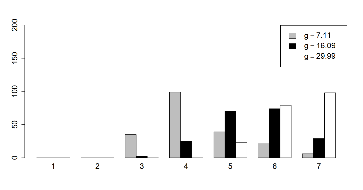
n=200

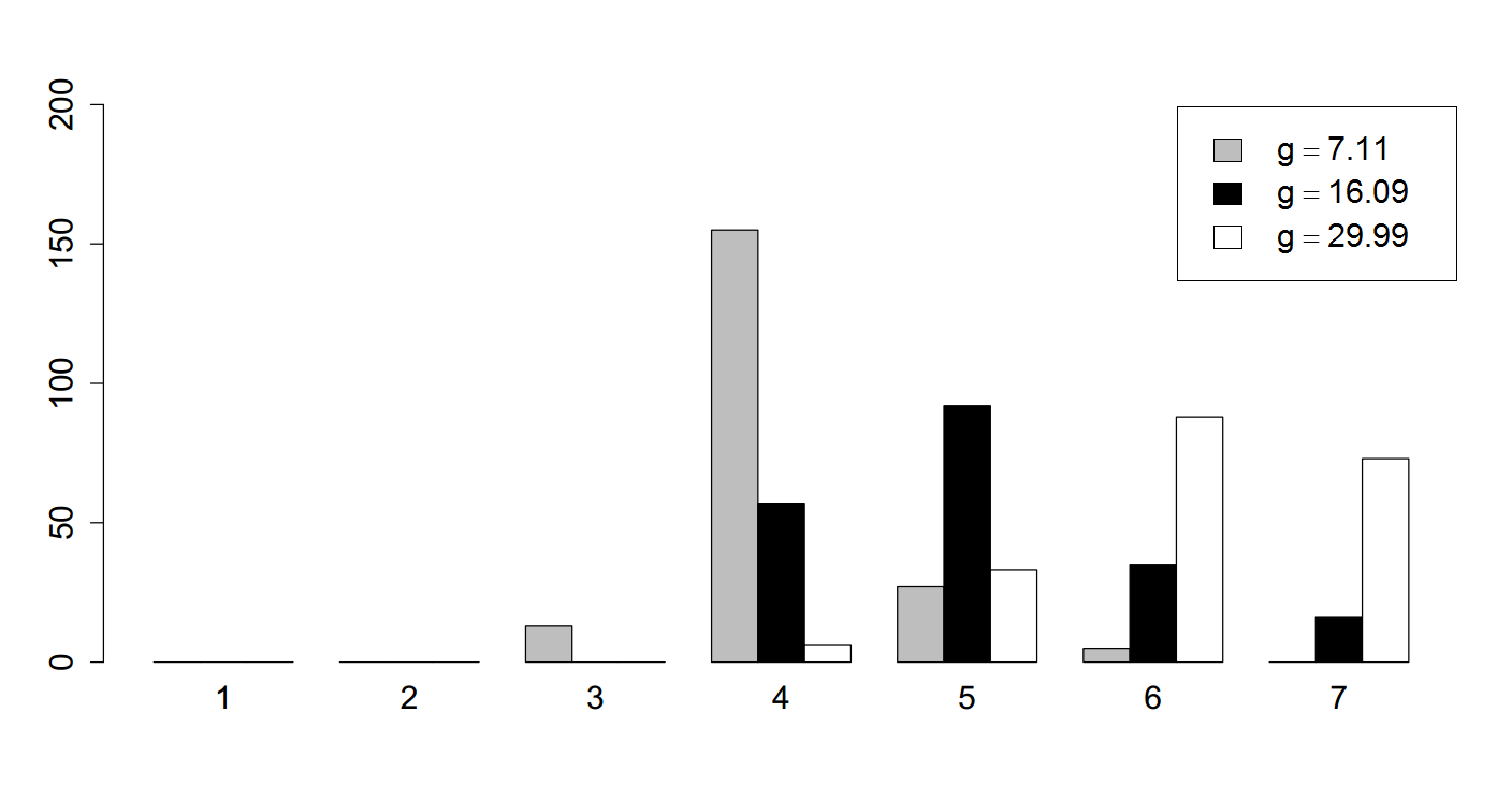
n=500

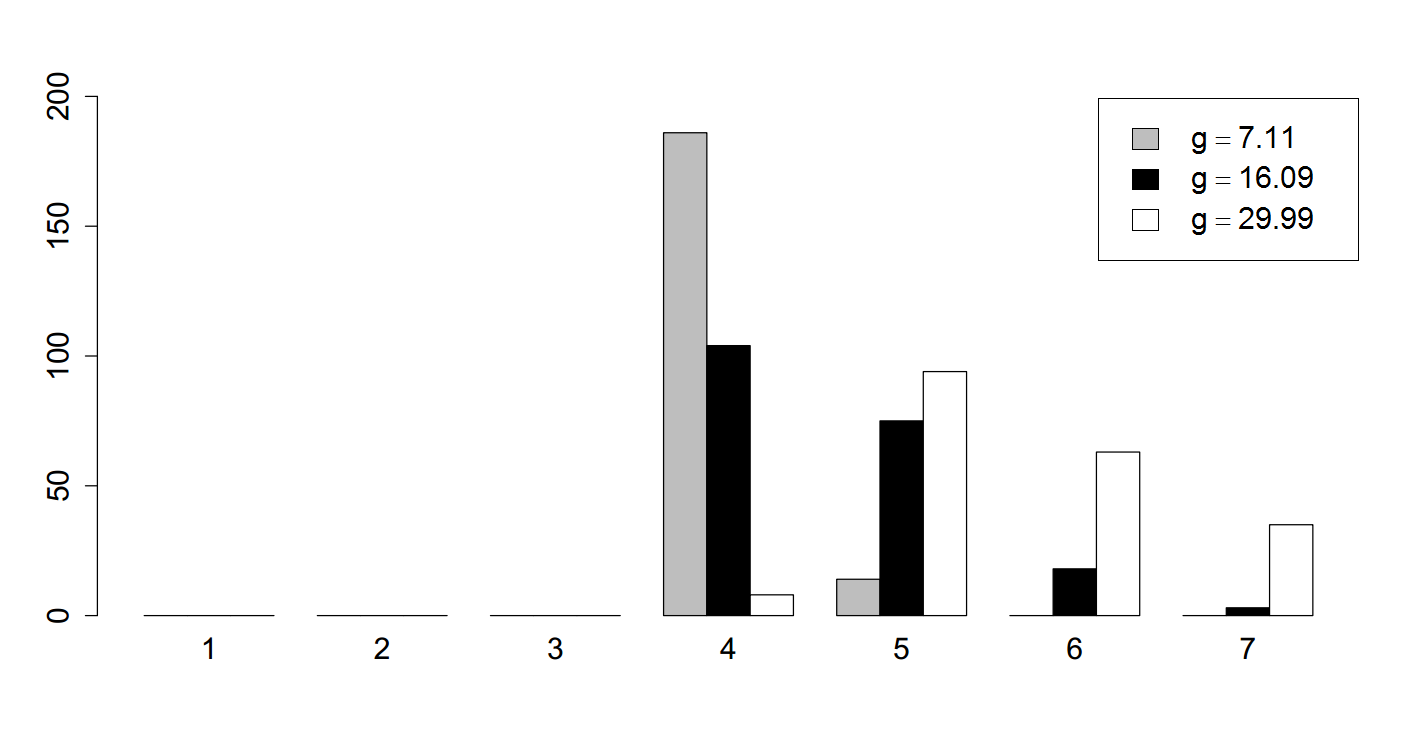
Figure S3. Binomial mixture. Frequencies of $\hat{k}$ for MOM-Beta for $g=7.11$, $g=16.09$ and $g=29.99$ with $q=2$. Results from 200 data sets with $n=50$, $n=200$ and $n=500$, $L=30$ and $k^{*}=4$

Figure S3 reproduces the Binomial mixture simulations from Section 4.7. Additionally to the default $g=7.11$ for the MOM-Beta prior, we now considered larger (more informative) $g=16.09,29.99$. Under these larger $g$ the performance remains competitive but does suffer, suggesting that the default $g=7.11$ is preferable. For a comparison to the BIC, sBIC and Beta priors see Figure 6.

S7. Comparison of ECP with other alternatives

We simulated a single data set of $n=200$ observations from Cases 1 and 3 in Section 4.1 and computed 50 times $\hat{P}(\mathcal{M}_{k}\mid{\bf y})$ under Normal-IW-Dir priors using the ECP estimator and the Marin and Robert [2008] estimator given by (3.3). Figures S4-S5 show that the medians of the ECP estimator and the Marin and Robert [2008] estimator with $k=\{1,...,4\}$ are similar, but that the ECP estimator produces higher precision estimates. To compute $\hat{P}(\mathcal{M}_{k}\mid{\bf y})$ using the ECP estimator we implement the bfnormmix function given in the R package mombf [Rossell et al., 2018].

$\hat{P}(\mathcal{M}_{1}\mid{\bf y})$	$\hat{P}(\mathcal{M}_{2}\mid{\bf y})$
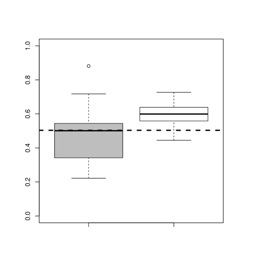
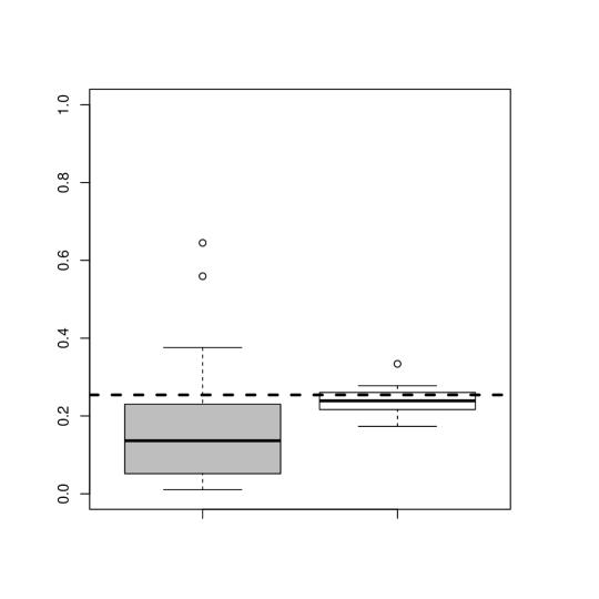
$\hat{P}(\mathcal{M}_{3}\mid{\bf y})$	$\hat{P}(\mathcal{M}_{4}\mid{\bf y})$

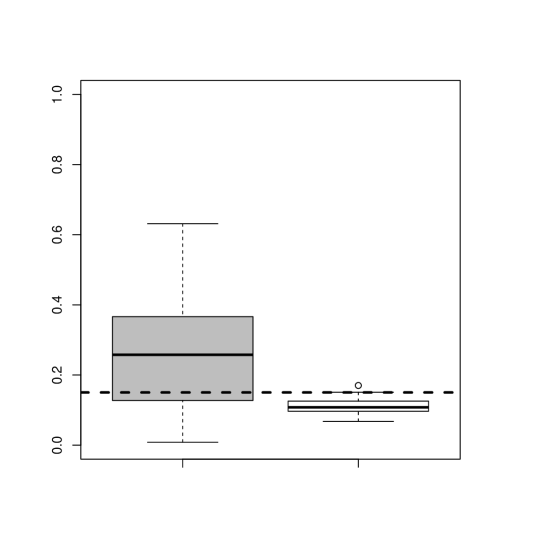
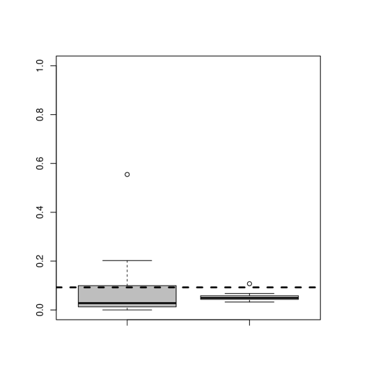
Figure S4. Boxplots display 50 independent estimates based on separate MCMC runs ($T=10,000$ iterations after a $T/10$ burn-in each). Precision of $\hat{P}(\mathcal{M}_{k}\mid{\bf y})$ under Normal-IW-Dir using the Marin and Robert [2008] estimator (gray) and ECP estimator (white) for $n=200$ observations in simulation Case 1. Dashed line indicate $\hat{P}(\mathcal{M}_{k}\mid{\bf y})$ under Normal-IW-Dir obtained by simulating $1,000,000$ values from the prior and averaging the likelihood.

$\hat{P}(\mathcal{M}_{1}\mid{\bf y})$	$\hat{P}(\mathcal{M}_{2}\mid{\bf y})$
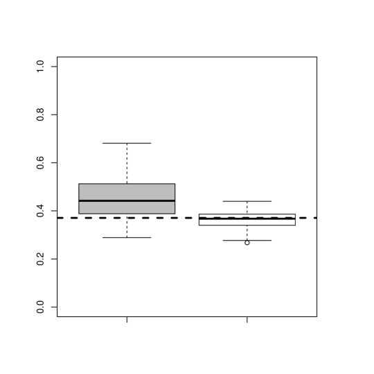
$\hat{P}(\mathcal{M}_{3}\mid{\bf y})$	$\hat{P}(\mathcal{M}_{4}\mid{\bf y})$

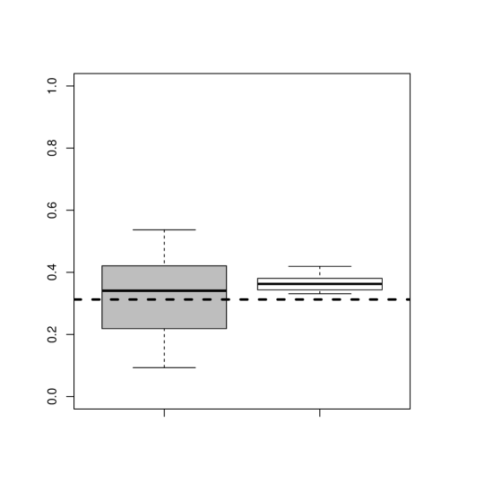
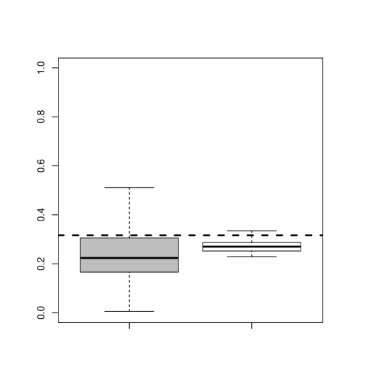
Figure S5. Boxplots display 50 independent estimates based on separate MCMC runs ($T=10,000$ iterations after a $T/10$ burn-in each). Precision of $\hat{P}(\mathcal{M}_{k}\mid{\bf y})$ under Normal-IW-Dir using the Marin and Robert [2008] estimator (gray) and ECP estimator (white) for $n=200$ observations in simulation Case 3. Dashed line indicate $\hat{P}(\mathcal{M}_{k}\mid{\bf y})$ under Normal-IW-Dir obtained by simulating $1,000,000$ values from the prior and averaging the likelihood.

S8. Precision of the Monte Carlo-estimated integrated likelihood

We compared empirically the precision of $\hat{p}({\bf y}\mid\mathcal{M}_{k})$ vs. the local prior-based $\tilde{p}({\bf y}\mid\mathcal{M}_{k})$ (Section 3.1) for univariate and bivariate Normal mixture and $k=2,3$ components (if $k=1$ then $p({\bf y}\mid\mathcal{M}_{k})=\tilde{p}({\bf y}\mid\mathcal{M}_{k})$ has closed form). To inspect whether the precision of $\hat{p}({\bf y}\mid\mathcal{M}_{k})$ suffers under overfitted mixtures we simulated a single data set of $n=500$ observations from a $k^{*}=1$ component mixture and computed 100 times both $\hat{p}({\bf y}\mid\mathcal{M}_{k})$ and $\tilde{p}({\bf y}\mid\mathcal{M}_{k})$. Figures S6 and S7 show the results for a univariate and bivariate outcome respectively. The precision of $\hat{p}({\bf y}\mid\mathcal{M}_{k})$ was comparable to that of $\tilde{p}({\bf y}\mid\mathcal{M}_{k})$, in fact in some situations the former was more precise (this is due to $\mbox{Var}(\log{\hat{p}})=\mbox{Var}(\log\tilde{p})+\mbox{Var}(\log\hat{\omega})+2\mbox{cov}(\log\tilde{p},\log\hat{\omega})$ where the latter covariance may be negative). More importantly, posterior model probabilities $\hat{p}(\mathcal{M}_{k}\mid{\bf y})$ (middle panels) were more precise than $\tilde{p}(\mathcal{M}_{k}\mid{\bf y})$, as in our experience tends to be the case due to $p(\mathcal{M}_{k}\mid{\bf y})$ having a higher concentration around 0 or 1 (Theorem 1). The lower panels show that as $k$ grows larger than $k^{*}$ the precision in $\hat{w}$ tends to degrade, however as mentioned this is compensated by the fact that $p(\mathcal{M}_{k}\mid{\bf y})$ is small for large $k$ (middle panels), thus it does not appear to be a practical concern.

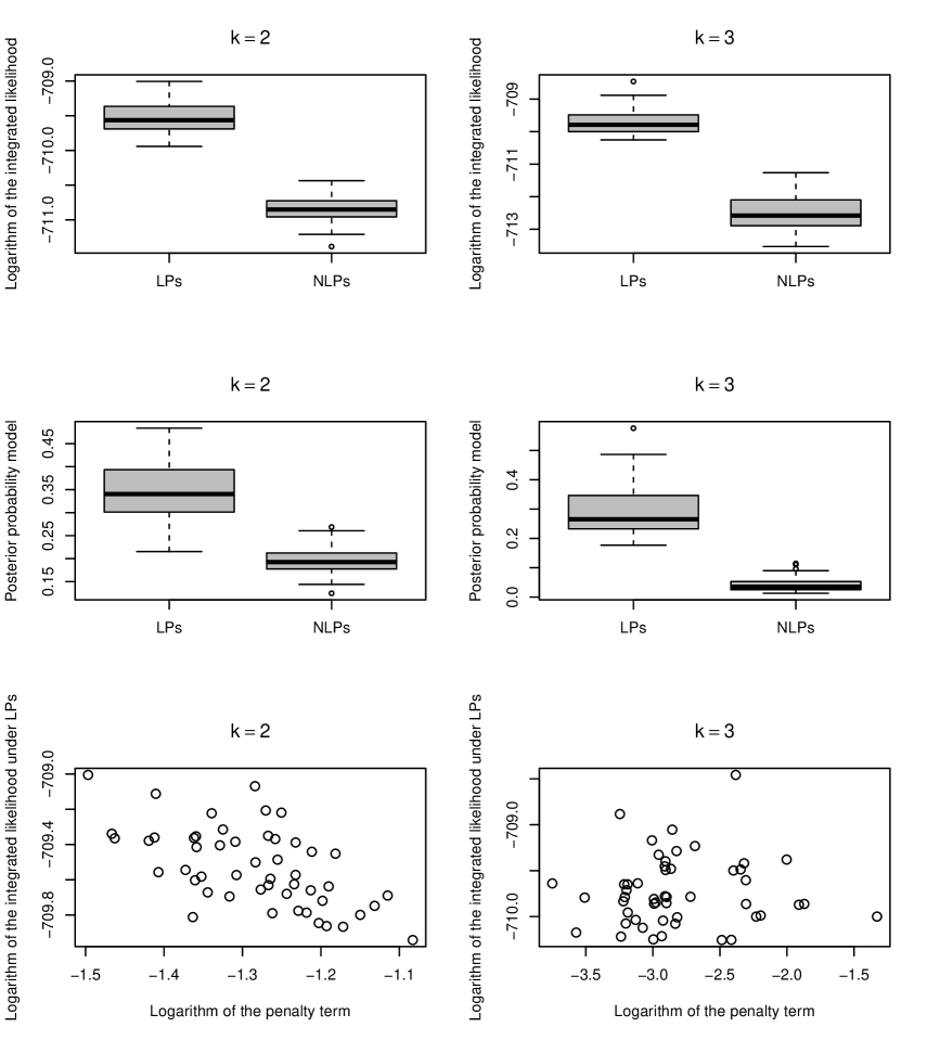
Figure S6. Precision of $\hat{p}({\bf y}\mid\mathcal{M}_{k})$ in 100 univariate simulations, $k^{*}=1$. Top: $\log\hat{p}({\bf y}\mid\mathcal{M}_{k})$. Middle: $\hat{p}(\mathcal{M}_{k}\mid{\bf y})$. Bottom: $\log\tilde{p}({\bf y}\mid\mathcal{M}_{k})$ vs. $\log\hat{E}(d_{\vartheta}(\bm{\vartheta}_{k})\mid{\bf y})$

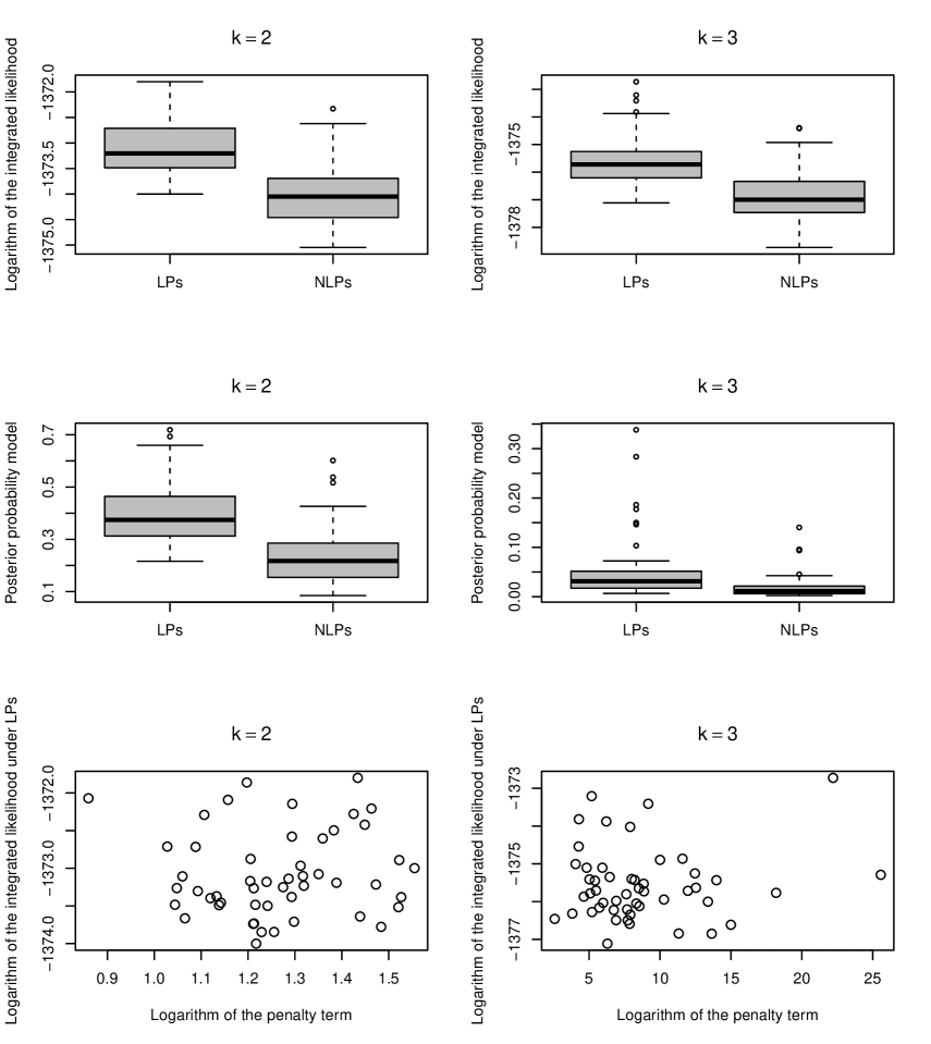
Figure S7. Precision of $\hat{p}({\bf y}\mid\mathcal{M}_{k})$ in 100 bivariate simulations, $k^{*}=1$. Top: $\log\hat{p}({\bf y}\mid\mathcal{M}_{k})$. Middle: $\hat{p}(\mathcal{M}_{k}\mid{\bf y})$. Bottom: $\log\tilde{p}({\bf y}\mid\mathcal{M}_{k})$ vs. $\log\hat{E}(d_{\vartheta}(\bm{\vartheta}_{k})\mid{\bf y})$

$n=200$	$n=1000$

S9. Gibbs sampling algorithms

Algorithm S2 outlines a Gibbs sampling algorithm for Normal mixtures under the Normal-IW-Dir prior

$$\mbox{Dir}(\bm{\eta};q)\prod_{j}N(\bm{\mu}_{j};0,g\Sigma_{j})\mbox{IW}(\Sigma_{j};\nu,S).$$

Analogously, Algorithm S3 outlines a Gibbs sampling algorithm for product Binomial mixtures under the Beta-Dirichlet prior

$$\mbox{Dir}(\bm{\eta};q)\prod_{jf}\mbox{Beta}\left(\theta_{jf};ag,(1-a)g\right).$$

1 Initialize $\bm{\vartheta}_{k}^{(0)}=(\bm{\theta}_{1}^{(0)},...,\bm{\theta}_{k}^{(0)},\bm{\eta}^{(0)})$ with $\bm{\theta}_{j}^{(0)}=(\bm{\mu}_{j}^{(0)},\Sigma_{j}^{(0)})$. for $t=1,...,T$ do

2       Draw $z_{i}^{(t)}=j$ with probability:

$$\dfrac{\eta^{(t-1)}_{k}N({\bf y}_{i};\bm{\mu}_{j}^{(t-1)},\Sigma_{j}^{(t-1)})}{\sum_{j=1}^{k}\eta^{(t-1)}_{j}N({\bf y}_{i};\bm{\mu}_{j}^{(t-1)},\Sigma_{j}^{(t-1)})}.$$

3      Let $n_{j}^{(t)}=\sum_{i=1}^{n}\mbox{I}(z_{i}^{(t)}=j)$ and $\bar{{\bf y}}_{j}^{(t)}=\dfrac{1}{n_{j}}\sum_{z_{i}^{(t)}=j}{\bf y}_{i}$ if $n_{j}^{(t)}>0$, else $\bar{{\bf y}}_{j}^{(t)}=0$. Draw

$$\bm{\eta}^{(t)} \sim\text{Dir}(q+n_{1}^{(t)},...,q+n_{k}^{(t)}).$$

4      Let $S_{j}=S^{-1}+\sum_{z_{i}=j}({\bf y}_{i}-\bar{{\bf y}}_{j}^{(t-1)})({\bf y}_{i}-\bar{{\bf y}}_{j}^{(t-1)})^{{}^{\prime}}+\sum_{j=1}^{k}\dfrac{n_{j}/g}{n_{j}+1/g}\bar{{\bf y}}_{j}^{(t)}\bar{{\bf y}}_{j}^{{}^{\prime}(t)}$. Draw

5      

$$\Sigma^{(t)}_{j}\sim\text{IW}\left(\nu+n_{j},S_{j}\right),$$

6      Draw

$$\bm{\mu}_{j}^{(t)}\sim N\left(\dfrac{gn_{j}^{(t)}\bar{{\bf y}}_{j}^{(t)}}{1+gn_{j}^{(t)}},\dfrac{g}{1+gn_{j}^{(t)}}\Sigma_{j}^{(t)}\right),$$

7 end for

Algorithm S 2 Gibbs sampling for Normal mixtures under a Normal-IW-Dir prior.

1Initialize $\bm{\vartheta}_{k}^{(0)}=(\bm{\theta}_{1}^{(0)},...,\bm{\theta}_{k}^{(0)},\bm{\eta}^{(0)})$ where $\bm{\theta}_{j}^{(0)}=(\theta_{j1}^{(0)},\ldots,\theta_{jp}^{(0)})$. for $t=1,...,T$ do

2       Draw $z_{i}^{(t)}=j$ with probability:

$$\dfrac{\eta^{(t-1)}_{j}\prod_{f=1}^{p}\text{Bin}(y_{if};L_{if},\theta_{jf}^{(t-1)})}{\sum_{j=1}^{k}\eta^{(t-1)}_{j}\prod_{f=1}^{p}\text{Bin}(y_{if};L_{if},\theta_{jf}^{(t-1)})}.$$

Draw

$$\bm{\eta}^{(t)} \sim\text{Dir}(q+n_{1}^{(t)},...,q+n_{k}^{(t)}).$$

where $n_{j}^{(t)}=\sum_{i=1}^{n}\mbox{I}(z_{i}^{(t)}=j)$. Draw

$$\theta_{jf}^{(t)}\sim\text{Beta}\left(ag+\sum_{z_{i}^{(t)}=j}y_{if},(1-a)g+\sum_{z_{i}^{(t)}=j}(L_{if}-y_{if})\right),$$

3 end for

Algorithm S 3 Gibbs sampling for product Binomial mixtures under the Beta-Dir prior.

S10. EM algorithm for multivariate Normal mixtures under MOM-Wishart-Dirichlet priors

The complete-data posterior can be written as follows

(S1) $$p(\bm{\vartheta}_{k}\mid{\bf y},{\bf z},\mathcal{M}_{k})=\prod_{j=1}^{k}\prod_{i=1}^{n}(\eta_{j}N({\bf y};\bm{\mu}_{j},\Sigma_{j}))^{z_{ij}}N\left(\bm{\mu}_{j};\bm{0},gA_{\Sigma}\right)\text{Wishart}(\Sigma_{j}^{-1};\nu,S)\mbox{Dir}(\bm{\eta};q).$$

The E-step at iteration $t$ requires the expectation of $\log p(\bm{\vartheta}_{k}\mid{\bf y},{\bf z},\mathcal{M}_{k})$ with respect to $p({\bf z}\mid{\bf y},\bm{\vartheta}_{k}^{(t-1)},\mathcal{M}_{k})$, where $\bm{\vartheta}_{k}^{(t-1)}=(\bm{\eta}^{(t-1)},\bm{\mu}_{1}^{(t-1)},...,\bm{\mu}_{k}^{(t-1)},\Sigma_{1}^{(t-1)},...,\Sigma_{k}^{(t-1)})$ are the parameter values at iteration $t-1$. Let

(S2) $$\bar{z}^{(t)}_{ij}=p(z_{i}=j\mid{\bf y}_{i},\bm{\vartheta}_{k}^{(t-1)})=\dfrac{\eta_{j}^{(t-1)}N({\bf y}_{i};\bm{\mu}_{j}^{(t-1)},\Sigma_{j}^{(t-1)})}{\sum_{j=1}^{k}\eta_{j}^{(t-1)}N({\bf y}_{i};\bm{\mu}_{j}^{(t-1)},\Sigma_{j}^{(t-1)})},$$

then the M-step seeks $\bm{\vartheta}_{k}^{(t)}$ maximising

(S3) $$\small\log(p(\bm{\vartheta}_{k}\mid{\bf y},\bar{z}_{ij},\mathcal{M}_{k}))= \sum_{j=1}^{k}n_{j}\log(\eta_{j})+\sum_{j=1}^{k}\sum_{i=1}^{n}\bar{z}_{ij}\log(N(\bm{y}_{i};\bm{\mu_{j}},\Sigma_{j}))+\sum_{j=1}^{k}\log(N\left(\bm{\mu}_{j};\bm{0},gA_{\Sigma}\right))$$

$$+\sum_{1\leq i<j\leq k}\log((\bm{\mu}_{i}-\bm{\mu}_{j})^{{}^{\prime}}A_{\Sigma}^{-1}(\bm{\mu}_{i}-\bm{\mu}_{j}))+\sum_{j=1}^{k}\log(\text{Wishart}(\Sigma_{j}^{-1};\nu,S))$$

$$+\log(\mbox{Dir}(\bm{\eta};q))$$

where $n_{j}^{(t)}=\sum_{i=1}^{n}\bar{z}^{(t)}_{ij}$. We successively update $\bm{\eta}^{(t)}$, $\bm{\mu}_{1}^{(t)}$,…,$\bm{\mu}_{k}^{(t)}$ and $\Sigma_{1}^{(t)},...,\Sigma_{k}^{(t)}$ in a fashion that guarantees that (S3) increases at each step. The update $\eta^{(t)}_{j}$ is

(S4) $$\eta^{(t)}_{j}=\dfrac{n_{j}^{(t)}+q-1}{n+k(q-1)},$$

which maximizes (S3) with respect to $\bm{\eta}$ conditional on the current $\bm{\mu}_{1}^{(t-1)}$,…,$\bm{\mu}_{k}^{(t-1)}$ and $\Sigma_{1}^{(t-1)},...,\Sigma_{k}^{(t-1)}$. To update $\bm{\mu}_{j}^{(t)}$ we seek to maximize

$$\xi(\bm{\mu}_{j}^{(t)})=\sum_{i\neq j}\log(\bm{C}_{ij}^{(t)^{\prime}}A_{\Sigma^{(t-1)}}^{-1}\bm{C}_{ij}^{(t)})-\dfrac{1}{2g}\bm{\mu}_{j}^{{}^{\prime}(t)}A_{\Sigma^{(t-1)}}^{-1}\bm{\mu}_{j}^{(t)}-\dfrac{1}{2}\sum_{i=1}^{n}\bar{z}^{(t)}_{ij}(\bm{y}_{i}-\bm{\mu}_{j}^{(t)})^{{}^{\prime}}A_{\Sigma^{(t-1)}}^{-1}(\bm{y}_{i}-\bm{\mu}_{j}^{(t)}),$$

where $\bm{C}_{ij}=(\bm{\mu}_{i}-\bm{\mu}_{j})$. The first derivative of $\xi(\bm{\mu}_{j}^{(t)})$ is

$$\nabla\xi(\bm{\mu}_{j}^{(t)}) =-2\sum_{i\neq j}\dfrac{A_{\Sigma^{(t-1)}}^{-1}\bm{C}_{ij}^{(t)}}{\bm{C}_{ij}^{(t)^{\prime}}A_{\Sigma^{(t-1)}}^{-1}\bm{C}_{ij}^{(t)}}-\dfrac{1}{g}(A_{\Sigma^{(t-1)}}^{-1}\bm{\mu}_{j}^{(t)})-\sum_{i=1}^{n}\bar{z}^{(t)}_{ij}(A_{\Sigma^{(t-1)}}^{-1}(\bm{y}_{i}-\bm{\mu}_{j}^{(t)})).$$

Because an analytic solution of $\nabla\xi(\bm{\mu}_{j}^{(t)})=\bm{0}$ in terms of $\bm{\mu}_{j}^{(t)}$ is not feasible we resort to a first order Taylor’s approximation for $-2\sum_{i\neq j}(A_{\Sigma^{(t-1)}}^{-1}\bm{C}_{ij}^{(t)})/(\bm{C}_{ij}^{(t)^{\prime}}A_{\Sigma^{(t-1)}}^{-1}\bm{C}_{ij}^{(t)})$ around $\bm{\mu}_{j}^{(t-1)}$. Finding the maximum of this Taylor approximation gives the candidate update

(S5) $$\bm{\mu}_{j}^{*}= \left(\Sigma_{j}^{-1(t-1)}n_{j}^{(t)}+A_{\Sigma^{(t-1)}}^{-1}\left(\dfrac{1}{g}+\sum_{\begin{subarray}{c}j\neq k\end{subarray}}\frac{2}{d_{ij}^{(t-1)}}\right)\right)^{-1}$$

$$\times\left(\Sigma^{-1(t-1)}n_{j}^{(t)}\bar{{\bf y}}_{j}^{(t)}+A_{\Sigma^{(t-1)}}^{-1}\left(\sum_{\begin{subarray}{c}i\neq j\end{subarray}}\frac{\bm{\mu}_{j}^{(t-1)}-(\bm{\mu}_{i}^{(t-1)}-\bm{\mu}_{j}^{(t-1)})}{d_{ij}^{(t-1)}}\right)\right),$$

where $d_{ij}^{(t-1)}=(\bm{\mu}_{i}^{(t-1)}-\bm{\mu}_{j}^{(t-1)})^{\prime}A_{\Sigma^{(t-1)}}^{-1}(\bm{\mu}_{i}^{(t-1)}-\bm{\mu}_{j}^{(t-1)})$. If $\xi(\bm{\mu}_{j}^{*})>\xi(\bm{\mu}_{j}^{(t-1)})$ we set $\bm{\mu}_{j}^{(t)}=\bm{\mu}_{j}^{*}$, else take the gradient step in Algorithm S4.

Finally we describe updating $\Sigma_{j}$ for $j=1,\ldots,k$. Redefine $\xi(\Sigma_{j})$ to now be (S3) viewed as a function of $\Sigma_{j}$. Due to the terms $\sum_{\begin{subarray}{c}i\neq j\end{subarray}}\log(\bm{\mu}_{i}^{(t)}-\bm{\mu}_{j}^{(t)})^{{}^{\prime}}A_{\Sigma^{(t)}}^{-1}(\bm{\mu}_{i}^{(t)}-\bm{\mu}_{j}^{(t)})$ and $-\frac{1}{2}\log(|A_{\Sigma^{(t)}}^{-1}|)$ an analytic solution of $\nabla\xi(\Sigma_{j})={\bf 0}$ is not available, hence we use the Taylor expansion around $\Sigma_{j}^{(t-1)}$

$$\small\sum_{\begin{subarray}{c}i\neq j\end{subarray}}\log(\bm{\mu}_{i}^{(t)}-\bm{\mu}_{j}^{(t)})^{{}^{\prime}}A_{\Sigma^{(t)}}^{-1}(\bm{\mu}_{i}^{(t)}-\bm{\mu}_{j}^{(t)})-\frac{1}{2}\log(|A_{\Sigma^{(t)}}^{-1}|)\approx$$

$$\sum_{\begin{subarray}{c}i\neq j\end{subarray}}\frac{(\bm{\mu}_{i}^{(t)}-\bm{\mu}_{j}^{(t)})^{{}^{\prime}}A_{\Sigma^{(t)}}^{-1}(\bm{\mu}_{i}^{(t)}-\bm{\mu}_{j}^{(t)})}{(\bm{\mu}_{i}^{(t-1)}-\bm{\mu}_{j}^{(t-1)})^{{}^{\prime}}A_{\Sigma^{(t-1)}}^{-1}(\bm{\mu}_{i}^{(t-1)}-\bm{\mu}_{j}^{(t-1)})}-\frac{1}{2}\log(|\Sigma_{j}^{(t)}|).$$

Note that when a common $\Sigma_{1}=\ldots=\Sigma_{k}$ is assumed then $A_{\Sigma^{(t)}}=\Sigma^{(t)}$ we only need a Taylor expansion of first term. Summarising, the candidate update is

$$(\nu-p+n_{j}^{(t)})\Sigma^{*}_{j}=S^{-1}+\dfrac{\bm{\mu}_{j}^{(t)}(\bm{\mu}_{j}^{(t)})^{\prime}}{kg}+\sum_{i=1}^{n}\bar{z}^{(t)}_{ij}({\bf y}_{i}-\bm{\mu}_{j}^{(t)})({\bf y}_{i}-\bm{\mu}_{j}^{(t)})^{{}^{\prime}}$$

$$-\dfrac{1}{k}\sum_{\begin{subarray}{c}i\neq j\end{subarray}}\dfrac{2(\bm{\mu}_{j}^{(t)}-\bm{\mu}_{k}^{(t)})(\bm{\mu}_{j}^{(t)}-\bm{\mu}_{k}^{(t)})^{{}^{\prime}}}{d_{ij}^{(t-1)}}.$$

If $\xi(\Sigma_{j}^{*})>\xi(\Sigma_{j}^{(t-1)})$ we set $\Sigma_{j}^{(t)}=\Sigma_{j}^{*}$, else take a gradient step (Algorithm S4) with a small enough step size to ensure that $\Sigma_{j}^{(t)}$ remains positive-definite.

1

2Initialization $\bm{\zeta}=\bm{\zeta}^{*}$, $\bar{k}=\sqrt{\dfrac{\|\bm{\zeta}^{*}-\bm{\zeta}^{(t-1)}\|}{\nabla\xi(\bm{\zeta}^{(t-1)})}}$ and $h=0$;

3 while $(\xi(\bm{\zeta}^{(t-1)})>\xi(\bm{\zeta}^{*}))$ do

4       $\bm{\zeta}^{*}=\bm{\zeta}^{(t-1)}+\dfrac{\bar{k}}{2^{h}}\nabla\xi(\bm{\zeta}^{(t-1)})$;

5       $h=h+1$

6 end while

$\bm{\zeta}^{(t)}=\bm{\zeta}^{*}$

Algorithm S 4 Gradient Ascend algorithm.

S11. EM algorithm for product Binomial mixture under MOM-Beta priors

The EM algorithm is derived analogously to that for Normal mixtures (Supplementary Section S10), and is described in Algorithm S5.

1 Set $t=1$. while $\zeta>\epsilon^{*}$ and $t<T$ do

2       for $t\geq 1$ and $j=1,...,k$ do

3             E-step. Let $\bar{z}^{(t)}_{ij}=\dfrac{\eta^{(t-1)}_{j}\prod_{f=1}^{p}\text{Bin}(y_{if};L_{if},\theta_{jf}^{(t-1)})}{\sum_{j=1}^{k}\eta^{(t-1)}_{j}\prod_{f=1}^{p}\text{Bin}(y_{if};L_{if},\theta_{jf}^{(t-1)})}.$ M-step. Update

$$\bm{\theta}_{j}^{(t)}=\dfrac{ag+\sum_{i=1}^{n}\bar{z}^{(t)}_{ij}{\bf y}_{i}+\ell_{1}(\bm{\theta}_{j}^{(t)})}{(1-a)g+\sum_{i=1}^{n}\bar{z}^{(t)}_{ij}(L_{if}-{\bf y}_{i})+2\ell_{2}(\bm{\theta}_{j}^{(t)})},$$

$\ell_{1}(\bm{\theta}_{j}^{(t)})=\dfrac{\bm{\theta}_{j}^{(t-1)}-(\bm{\theta}_{i}^{(t-1)}-\bm{\theta}_{j}^{(t-1)})}{(\bm{\theta}_{i}^{(t-1)}-\bm{\theta}_{j}^{(t-1)})^{\prime}(\bm{\theta}_{i}^{(t-1)}-\bm{\theta}_{j}^{(t-1)})},$ $\ell_{2}(\bm{\theta}_{j}^{(t)})=\left[(\bm{\theta}_{i}^{(t-1)}-\bm{\theta}_{j}^{(t-1)})^{\prime}(\bm{\theta}_{i}^{(t-1)}-\bm{\theta}_{j}^{(t-1)})\right]^{-1}.$ Update $\eta^{(t)}_{j}=\dfrac{n_{j}^{(t)}+q-1}{n+k(q-1)}$.

4       end for

5      Compute $\zeta=|\xi(\bm{\vartheta}_{k}^{(t)})-\xi(\bm{\vartheta}_{k}^{(t-1)})|$ and set $t=t+1$.

6 end while

Algorithm S 5 EM under MOM-Beta priors.

S12. Sensitivity to prior elicitation

We provide additional results for the simulation study in Section 4.1.

Regarding the univariate Normal mixtures in Cases 1-4, the four top panels in Figure S10 show the posterior expected number of components given by $E(k\mid{\bf y})=P(\mathcal{M}_{1}\mid{\bf y})+2P(\mathcal{M}_{2}\mid{\bf y})+3P(\mathcal{M}_{3}\mid{\bf y})$ for the alternative prior specification $q=2$ and $P(\kappa<4)=0.05$. The four top panels in Figure S11 show analogous results for $q=4$ and $P(\kappa<4)=0.05$, showing that the findings are fairly robust to mild deviations from our default $q$.

Regarding the bivariate Normal mixtures in Cases 5-8, the four bottom panels in Figure S10 shows $E(k\mid{\bf y})$ for $q=3$ and $P(\kappa<4)=0.05$. The four bottom panels in Figure S11 show the same results for $q=16.5$ (a value recommended in Frühwirth-Schnatter [2006] and Mengersen et al. [2011], Chapter 10) and $P(\kappa<4)=0.05$, showing again that the findings are fairly robust to mild deviations from our recommended prior setting.

Finally, to assess sensitivity to the prior elicitation of $g$, Figure S13 shows the average posterior probability $P(\mathcal{M}_{k^{*}}\mid{\bf y})$ for Cases 1-8 with $P(\kappa<4)=0.1$ and $q$ set as in Figure 2. Although the results are largely similar to those in Figure 2, the benefits in parsimony enforcement are somewhat reduced in some situations (e.g. Case 5), indicating that $P(\kappa<4\mid g,\mathcal{M}_{K})=0.05$ may be slightly preferable to 0.1 to achieve a better balance between parsimony and detection power.

Case 1 ($k^{*}=1$, q=2)	Case 2 ($k^{*}=2$, p=1, q=2)
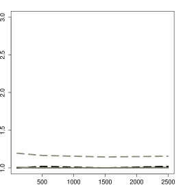
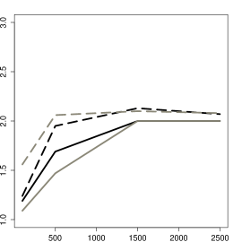
Case 3 ($k^{*}=2$, p=1, q=2)	Case 4 ($k^{*}=3$, p=1, q=2)
Case 5 ($k^{*}=1$, p=2, q=3)	Case 6 ($k^{*}=2$, p=2, q=3)
Case 7 ($k^{*}=2$, p=2, q=3)	Case 8 ($k^{*}=3$, p=2, q=3)

Figure S10. Simulation study. Posterior expected model size $E(k\mid{\bf y})$ versus $n$ for $q=p+1$ for the MOM-IW-Dir (solid line) and Normal-IW-Dir (dotted line).

Case 1 ($k^{*}=1$, q=4)	Case 2 ($k^{*}=2$, p=1, q=4)
Case 3 ($k^{*}=2$, p=1, q=4)	Case 4 ($k^{*}=3$, p=1, q=4)
Case 5 ($k^{*}=1$, p=2, q=16.5)	Case 6 ($k^{*}=2$, p=2, q=16.5)
Case 7 ($k^{*}=2$, p=2, q=16.5)	Case 8 ($k^{*}=3$, p=2, q=16.5)

Figure S11. Simulation study. Posterior expected model size $E(k\mid{\bf y})$ versus $n$ for $q=4$ and $q=16.5$ for univariate and bivariate Normal mixtures as recommended by Frühwirth-Schnatter [2006] for the MOM-IW-Dir (solid line) and Normal-IW-Dir (dotted line).

Case 1 ($k^{*}=1$, q=2)	Case 2 ($k^{*}=2$, p=1, q=2)
Case 3 ($k^{*}=2$, p=1, q=2)	Case 4 ($k^{*}=3$, p=1, q=2)
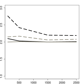
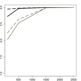
Case 5 ($k^{*}=1$, p=2, q=3)	Case 6 ($k^{*}=2$, p=2, q=3)
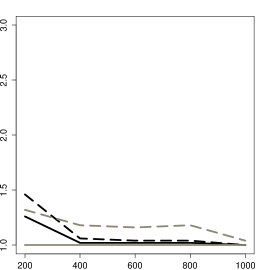
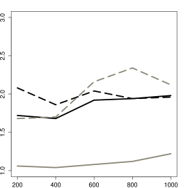
Case 7 ($k^{*}=2$, p=2, q=3)	Case 8 ($k^{*}=3$, p=2, q=3)

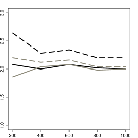
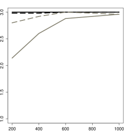
Figure S12. Simulation study. Average $\hat{k}$ versus $n$ for MOM-IW-Dir (solid black), Normal-IW-Dir (dotted black), AIC (dotted gray) and BIC (solid gray).

Case 1 ($k^{*}=1$, p=1, q=2)	Case 2 ($k^{*}=2$, p=1, q=2)
Case 3 ($k^{*}=2$, p=1, q=2)	Case 4 ($k^{*}=3$, p=1, q=2)
Case 5 ($k^{*}=1$, p=2, q=3)	Case 6 ($k^{*}=2$, p=2, q=3)
Case 7 ($k^{*}=2$, p=2, q=3)	Case 8 ($k^{*}=3$, p=2, q=3)

Figure S13. Simulation study. $P(\mathcal{M}_{k^{*}}\mid{\bf y})$ versus $n$ under $P(\kappa<4\mid\mathcal{M}_{k})=0.1$ for the MOM-IW-Dir (solid line) and Normal-IW-Dir (dotted line).

S13. Supplementary results for the applications

Table S4 provides more detailed results for the misspecified Normal model (Section 4.2). It indicates the posterior probability of 11 models with $k=1,...,6$ components, for each $k$, considering either homogeneous ($\Sigma_{j}=\Sigma$) or heterogeneous ($\Sigma_{i}\neq\Sigma_{j}$) covariance matrices. The model with highest posterior, BIC and AIC is indicated in bold face. Table S6 shows analogous results for the Faithful data (Section 4.4), Table S7 for the Iris data (Section 4.5) and Table S5 for the Cytometry data (Section 4.3).

As an alternative to formal Bayesian model selection suppose one fits a model with a large number of components ($k=6$ in our examples) to successively discard those deemed unnecessary. One strategy to discard components is to set a threshold on the estimated $\hat{\bm{\eta}}$, which results in the addition of spurious components. An alternative illustrated in Table 2 and Table S8 is to describe the number $m=\sum_{j=1}^{k}\mbox{I}(n_{j}>0)$ of non-empty components (no allocated observations) at each MCMC iteration when obtaining posterior draws from $p^{L}({\bf z},\bm{\vartheta}\mid{\bf y},\mathcal{M}_{6})$ and $p({\bf z},\bm{\vartheta}\mid{\bf y},\mathcal{M}_{6})$ (respectively). For instance, for the misspecified model roughly 95% of the MCMC iterations had 6 components with some allocated observations, and similarly for other data sets, which naively suggest that at least $k=6$ components are needed. This is in stark contrast with posterior model probabilities $P(\mathcal{M}_{k}\mid{\bf y})$ in Tables S4-S5, which suggest more parsimonious models. This difference is explained by the fact that $P(m\mid{\bf y},\mathcal{M}_{6})$ reported in Table 2 and Table S8 conditions on the larger model whereas $P(\mathcal{M}_{k}\mid{\bf y})$ is a formal measure of uncertainty for each of the models under consideration conditional on the observed data.

Table S4. Misspecified model. $P(\mathcal{M}_{k}\mid{\bf y})$ under Normal-IW-Dir and MOM-IW-Dir priors, BIC, AIC and sBIC for $k\in\{1,\ldots,6\}$ and homogeneous ($\Sigma_{j}=\Sigma$) or heterogeneous ($\Sigma_{i}\neq\Sigma_{j}$)

		Normal-IW-Dir	MOM-IW-Dir	BIC	AIC	sBIC
	$k$	$P(\mathcal{M}_{k}\mid{\bf y})$	$P(\mathcal{M}_{k}\mid{\bf y})$
	1	0.000	0.000	-2992.820	-2981.828
$\Sigma_{j}=\Sigma$	2	0.000	0.000	-2549.767	-2532.179
	3	0.003	1.000	-2548.774	-2524.591
	4	0.062	0.000	-2556.581	-2525.803
	5	0.469	0.000	-2566.122	-2528.748
	6	0.465	0.000	-2574.371	-2530.402
$\Sigma_{i}\neq\Sigma_{j}$	2	0.000	0.000	-2545.129	-2520.946	-2548.942
	3	0.000	0.000	-2529.037	-2491.663	-2534.729
	4	0.000	0.000	-2522.954	-2472.389	-2527.448
	5	0.000	0.000	-2535.703	-2471.948	-2528.207
	6	0.000	0.000	-2546.878	-2469.931	-2529.068

Table S5. Cytometry data. $P(\mathcal{M}_{k}\mid{\bf y})$ under Normal-IW-Dir and MOM-IW-Dir priors, BIC, AIC and sBIC for $k\in\{1,\ldots,6\}$ and homogeneous ($\Sigma_{j}=\Sigma$) or heterogeneous ($\Sigma_{i}\neq\Sigma_{j}$)

		Normal-IW-Dir	MOM-IW-Dir	BIC	AIC	sBIC
	$k$	$P(\mathcal{M}_{k}\mid{\bf y})$	$P(\mathcal{M}_{k}\mid{\bf y})$
	1	0.000	0.000	-28337.23	-28295.02
$\Sigma_{j}=\Sigma$	2	0.000	0.000	-27720.64	-27665.86
	3	0.000	0.000	-27541.73	-27474.39
	4	0.000	0.000	-27443.22	-27363.31
	5	0.000	0.000	-27271.67	-27179.19
	6	0.000	0.000	-27226.41	-27121.36
$\Sigma_{i}\neq\Sigma_{j}$	2	0.072	0.005	-27357.56	-27277.65	-37869.06
	3	0.928	0.995	-27015.35	-26897.74	-36478.20
	4	0.000	0.000	-27048.60	-26893.29	-35247.11
	5	0.000	0.000	-27041.50	-26848.50	-34415.96
	6	0.000	0.000	-27075.18	-26844.48	-33888.20

Table S6. Faithful data. $P(\mathcal{M}_{k}\mid{\bf y})$ under Normal-IW-Dir and MOM-IW-Dir priors, BIC, AIC and sBIC for $k\in\{1,\ldots,6\}$ and homogeneous ($\Sigma_{j}=\Sigma$) or heterogeneous ($\Sigma_{i}\neq\Sigma_{j}$)

		Normal-IW-Dir	MOM-IW-Dir	BIC	AIC	sBIC
	$k$	$P(\mathcal{M}_{k}\mid{\bf y})$	$P(\mathcal{M}_{k}\mid{\bf y})$
	1	0.000	0.000	-558.006	-548.992
$\Sigma_{j}=\Sigma$	2	0.000	0.000	-416.805	-402.382
	3	0.132	0.967	-411.356	-391.524
	4	0.473	0.000	-419.748	-394.507
	5	0.353	0.000	-418.019	-387.369
	6	0.042	0.000	-427.821	-391.763
$\Sigma_{i}\neq\Sigma_{j}$	2	0.000	0.000	-415.291	-395.459	-419.103
	3	0.000	0.000	-422.609	-391.960	-415.938
	4	0.000	0.000	-425.370	-383.903	-417.278
	5	0.000	0.000	-439.754	-387.470	-420.569
	6	0.000	0.000	-448.896	-385.795	-422.231

Table S7. Iris data. $P(\mathcal{M}_{k}\mid{\bf y})$ under Normal-IW-Dir and MOM-IW-Dir priors, BIC, AIC and sBIC for $k\in\{1,\ldots,6\}$ and homogeneous ($\Sigma_{j}=\Sigma$) or heterogeneous ($\Sigma_{i}\neq\Sigma_{j}$)

		Normal-IW-Dir	MOM-IW-Dir	BIC	AIC	sBIC
	$k$	$P(\mathcal{M}_{k}\mid{\bf y})$	$P(\mathcal{M}_{k}\mid{\bf y})$
	1	0.000	0.000	-414.989	-393.915
$\Sigma_{j}=\Sigma$	2	0.000	0.000	-344.049	-315.448
	3	0.809	1.000	-316.483	-280.355
	4	0.029	0.000	-295.705	-252.051
	5	0.132	0.000	-302.465	-251.284
	6	0.030	0.000	-310.909	-252.201
$\Sigma_{i}\neq\Sigma_{j}$	2	0.000	0.000	-287.009	-243.355	-415.449
	3	0.000	0.000	-290.420	-224.186	-410.122
	4	0.000	0.000	-314.483	-225.669	-408.839
	5	0.000	0.000	-341.910	-230.517	-414.190
	6	0.000	0.000	-355.786	-221.813	-422.209

Table S8. Posterior distribution on non-empty components $m=\sum_{j=1}^{k}\mbox{I}(n_{j}>0)$ in repulsive overfitted mixtures under $\Sigma_{j}=\Sigma$. The Misspecified, Faithful, Iris and cytometry data considered in Section 4.

	$\hat{P}(m\mid{\bf y},\mathcal{M}_{6})$
	$m=1$	$m=2$	$m=3$	$m=4$	$m=5$	$m=6$
			$q=1$
Misspecified	0.00	0.00	0.00	0.00	0.02	0.98
Faithful	0.00	0.00	0.00	0.00	0.26	0.74
Iris	0.00	0.99	0.00	0.01	0.00	0.00
Cytometry	0.00	0.00	0.00	0.00	0.00	1.00
			$q=0.01$
Misspecified	0.00	0.00	0.00	0.35	0.63	0.02
Faithful	0.00	0.00	0.76	0.23	0.01	0.00
Iris	0.00	1.00	0.00	0.00	0.00	0.00
Cytometry	0.00	0.00	0.00	0.00	0.00	1.00
			$q=3.10^{-8}$
Misspecified	0.00	0.00	0.83	0.00	0.00	0.17
Faithful	0.00	0.00	0.99	0.01	0.00	0.00
Iris	0.00	1.00	0.00	0.00	0.00	0.00
Cytometry	0.00	0.00	0.00	0.00	0.00	1.00

Table S9. Combined words in the political blogs data

clinton	clintons
obama	obamas	barack
america	american	americans
candidate	candidates
democratic	democrats
new	news
president	presidential
senate	senator
year	years
vote	voters
thing	things

Table S10. Political blogs data. $P(\mathcal{M}_{k}\mid{\bf y})$ under a MOM-Beta and Beta priors and $k\in\{1,\ldots,6\}$, BIC and BIC.

		MOM-Beta	Beta	BIC	AIC
	$k$	$P(\mathcal{M}_{k}\mid{\bf y})$	$P(\mathcal{M}_{k}\mid{\bf y})$
	1	0.000	0.000	-257405.2	-256317.0
	2	1.000	0.000	-255488.8	-253307.8
	3	0.000	0.000	-255329.7	-252055.9
	4	0.000	1.000	-255358.8	-250992.2
	5	0.000	0.000	-255712.2	-250252.7
	6	0.000	0.000	-256366.0	-249813.7

S14. Sample R code

The R code below generates bivariate data from a single-component Normal mixture and uses bfnormmix from R package mombf to obtain posterior probabilities for 1-3 components, both under MOM-IW-Dir and Normal-IW-Dir priors, under default prior parameters. The obtained estimates are $P(\mathcal{M}_{1}\mid{\bf y})=0.889$ and $0.771$ for MOM-IW-Dir and Normal-IW-Dir priors, respectively.

> library(mombf)
> set.seed(1)
>      x <- matrix(rnorm(100*2),ncol=2)
>      bfnormmix(x=x,k=1:3)
mixturebf object with 2 variables

Use draw() to obtain posterior samples. postProb() returns posterior probabilities as given below

  k   pp.momiw     pp.niw logprobempty logbf.momiw     logpen logbf.niw
1 1 0.88864310 0.77117451         -Inf    0.000000  0.0000000  0.000000
2 2 0.09992687 0.18573876    -3.191547   -2.185257 -0.7616836 -1.423573
3 3 0.01143003 0.04308673    -2.470700   -4.353451 -1.4687516 -2.884700
        model
1 Normal, VVV
2 Normal, VVV
3 Normal, VVV

S15. An illustration for the computations for the product of Binomial mixture under MOM-Beta priors

We illustrate some computational issues and diagnostics related to posterior multi-modality, the EM and MCMC algorithms in product Binomial mixtures. We considered a simulation with $k^{*}=4$ components, $n=500$, $p=8$ variables and equal component weights $\eta_{1}^{*}=\eta_{2}^{*}=\eta_{3}^{*}=\eta_{4}^{*}=1/4$. Each component had two large success probabilities $\theta_{jf}^{*}=0.32$ whereas the remaining probabilities were small (0.04 and 0.08), specifically

(S1) $$\bm{\theta} =\begin{pmatrix}0.32&0.04&0.04&0.04\\ 0.32&0.08&0.08&0.08\\ 0.04&0.32&0.04&0.04\\ 0.08&0.32&0.08&0.08\\ 0.04&0.04&0.32&0.04\\ 0.08&0.08&0.32&0.08\\ 0.04&0.04&0.04&0.32\\ 0.08&0.08&0.08&0.32\\ \end{pmatrix}.$$

The default MOM-Beta prior parameters are $g=2.6$ and $q=2$ (Section 2.3). Although our EM algorithm is guaranteed to increase the log-posterior at each iteration, in practice there are potential issues with slow convergence or reaching local maxima/saddlepoints. To address this in our implementation we run the EM algorithm (Algorithm 5) from 30 different random starting values and keep the estimate achieving the highest log-posterior value. The obtained estimates were fairly close to the simulation truth, specifically

(S2) $$\hat{\bm{\eta}} =(0.28,0.26,0.24,0.22); \hat{\bm{\theta}} =\begin{pmatrix}0.34&0.05&0.04&0.04\\ 0.28&0.07&0.08&0.07\\ 0.04&0.31&0.04&0.05\\ 0.08&0.31&0.08&0.08\\ 0.05&0.05&0.35&0.06\\ 0.09&0.08&0.31&0.08\\ 0.03&0.04&0.04&0.33\\ 0.09&0.09&0.07&0.30\\ \end{pmatrix}$$

We also studied the ability of the BIC, AIC, and Beta and MOM-Beta priors to recover $k^{*}=4$, finding that all except for the AIC returned the correct value (Table S11). Recall that the posterior probabilities require estimating the integrated likelihood, for which in turn we run an MCMC algorithm. To assess practical MCMC convergence we used trace plots for 2,000 iterations targetting $p(\bm{\vartheta}_{4}\mid{\bf y},\mathcal{M}_{4})$ after a burn period of 1,000. The plots did not reveal any issues with the chain’s mixing.

Table S11. Product Binomial simulation. $P(\mathcal{M}_{k}\mid{\bf y})$ for $k\in\{1,\ldots,6\}$ under Beta and MOM-Beta priors, BIC and AIC.

	Beta	MOM-Beta	BIC	AIC
$k$	$P(\mathcal{M}_{k}\mid{\bf y})$	$P(\mathcal{M}_{k}\mid{\bf y})$
1	0.000	0.000	-22702.00	-22668.29
2	0.000	0.000	-21569.65	-21498.00
3	0.000	0.000	-20782.58	-20673.00
4	1.000	1.000	-20051.63	-19904.11
5	0.000	0.000	-20074.65	-19889.21
6	0.000	0.000	-20099.17	-19875.80

References

- Affandi et al. [2013] R. H. Affandi, E. B. Fox, and B. Taskar. Approximate inference in continuous determinantal processes. In Advances in Neural Information Processing Systems, pages 1430–1438, 2013.
- Allman et al. [2009] E. S. Allman, C. Matias, and J. A. Rhodes. Identifiability of parameters in latent structure models with many observed variables. The Annals of Statistics, 37(6):3099–3132, 2009.
- Andrews [1998] G. E. Andrews. The theory of partitions. Number 2 in 1. Cambridge university press, 1998.
- Baudry et al. [2012] J. P. Baudry, A. E. Raftery, G. Celeux, K. Lo, and R. Gottardo. Combining mixture components for clustering. Journal of Computational and Graphical Statistics, 2012.
- Biernacki et al. [2000] C. Biernacki, G. Celeux, and G. Govaert. Assessing a mixture model for clustering with the integrated completed likelihood. IEEE transactions on pattern analysis and machine intelligence, 22(7):719–725, 2000.
- Brinkman et al. [2007] R. R. Brinkman, M. Gasparetto, J. Lee, A. J. Ribickas, J. Perkins, W. Janssen, R. Smiley, and C. Smith. High-content flow cytometry and temporal data analysis for defining a cellular signature of graft-versus-host disease. Biology of Blood and Marrow Transplantation, 13(6):691–700, 2007.
- Chambaz and Rousseau [2008] A. Chambaz and J. Rousseau. Bounds for Bayesian order identification with application to mixtures. The Annals of Statistics, 36:928–962, 2008.
- Chang [2015] J. Chang. lda: Collapsed Gibbs Sampling Methods for Topic Models, 2015. URL https://CRAN.R-project.org/package=lda. R package version 1.4.2.
- Chen and Li [2009] J. Chen and P. Li. Hypothesis test for Normal mixture models: The EM approach. The Annals of Statistics, 37:2523–2542, 2009.
- Chib [1995] S. Chib. Marginal likelihood from the Gibbs output. Journal of the American Statistical Association, 90:1313–1321, 1995.
- Collazo and Smith [2016] R.A. Collazo and J.Q. Smith. A new family of non-local priors for chain event graph model selection. Bayesian Analysis, 11(4):1165–1201, 2016.
- Consonni et al. [2013] G. Consonni, J.J. Forster, and L. La Rocca. The whetstone and the alum block: Balanced objective bayesian comparison of nested models for discrete data. Statistical Science, 28(3):398–423, 2013.
- Crawford [1994] S.L. Crawford. An application of the Laplace method to finite mixture distributions. Journal of the American Statistical Association, 89:259–267, 1994.
- Dawid [1999] A.P. Dawid. The trouble with Bayes factors. Technical report, University College London, 1999.
- Dempster et al. [1977] A.P. Dempster, N. M. Laird, and D. B. Rubin. Maximum Likelihood from Incomplete Data via the EM Algorithm. Journal of the Royal Statistical Society, B, 39-1:1–38, 1977.
- Došlá [2009] Š. Došlá. Conditions for bimodality and multimodality of a mixture of two unimodal densities. Kybernetika, 45(2):279–292, 2009.
- Drton and Plummer [2017] M. Drton and M. Plummer. A Bayesian information criterion for singular models. Journal of the Royal Statistical Society: Series B (Statistical Methodology), 79(2):323–380, 2017.
- Efron [2008] B. Efron. Microarrays, empirical Bayes and the two-groups model. Statistical Science, 23-1:1–22, 2008.
- Escobar and West [1995] M. Escobar and M. West. Bayesian density estimation and inference using mixtures. Journal of the American Statistical Association, 90:577–588, 1995.
- Fisher [1936] R. A. Fisher. The use of multiple measurements in taxonomic problems. Annals of Eugenics, 7:179–188, 1936.
- Fraley and Raftery [2002] C. Fraley and A. E. Raftery. Model-based clustering, discriminant analysis, and density estimation. Journal of the American Statistical Association, 97:611–631, 2002.
- Frühwirth-Schnatter [2006] S. Frühwirth-Schnatter. Finite Mixtures and Markov Switching Models. Springer, New York, 2006.
- Frühwirth-Schnatter [2004] Silvia Frühwirth-Schnatter. Estimating marginal likelihoods for mixture and Markov switching models using bridge sampling techniques. Mixtures: Estimation and Applications, pages 213–239, 2004.
- Gassiat and Handel [2013] E. Gassiat and R. Van Handel. Consistent order estimation and minimal penalties. IEEE Transactions on Information Theory, 59(2):1115–1128, 2013.
- Gelman et al. [2013] A. Gelman, J. B. Carlin, H. S. Stern, D. B. Dunson, A. Vehtari, and D. B. Rubin. Bayesian Data Analysis, Third Edition. Boca Raton: Chapman and Hall/CRC, 2013.
- Ghosal [2002] S. Ghosal. A review of consistency and convergence of posterior distribution. In Division of theoretical statistics and mathematics, pages 1–10, Indian Statistical Institute, 2002.
- Ghosal and der Vaart [2001] S. Ghosal and A. V. der Vaart. Entropies and rates of convergence for maximum likelihood and bayes estimation for mixture of normal densities. Annals of Statistics, 29:1233–1263, 2001.
- Ghosal and Van Der Vaart [2007] S. Ghosal and A. Van Der Vaart. Posterior convergence rates of dirichlet mixtures at smooth densities. The Annals of Statistics, 35:697–723, 2007.
- Ghosh and Sen [1985] J. K. Ghosh and P. K. Sen. On the asymptotic performance of the log-likelihood ratio statistic for the mixture model and related results. In Le Cam, L. M., Olshen, R. A. (Eds.), Proceedings of the Berkeley conference in Honor of Jerzy Neyman and Jack Kiefer, volume II, pages 789–806, Wadsworth, Monterey, 1985.
- Grün and Leisch [2008] B. Grün and F. Leisch. Finite mixtures of generalized linear regression models. In Shalabh and C. Heumann, editors, Recent advances in linear models and related areas, pages 205–230. Springer, 2008.
- Hathaway [1985] R. J. Hathaway. A constrained formulation of maximum-likelihood estimation for Normal mixture distributions. Annals of Statistics, 13:795–800, 1985.
- Havre et al. [2015] Z. V. Havre, N. White, J. Rousseau, and K. Mengersen. Overfitting bayesian mixture models with and unknown number of components. PLoS ONE, 10 (7):1–27, 2015.
- Heinzl and Tutz [2014] F. Heinzl and G. Tutz. Clustering in linear-mixed models with a group fused lasso penalty. Biometrical Journal, 56(1):44–68, 2014.
- Ho and Nguyen [2016] N. Ho and X. Nguyen. Convergence rates of parameter estimation for some weakly identifiable finite mixtures. Annals of Statistics, 44(6):2726–2755, 2016.
- Johnson and Rossell [2010] V. E. Johnson and D. Rossell. On the use of non-local prior densities in Bayesian hypothesis tests. Journal Royal Statistical Society, B, 72:143–170, 2010.
- Johnson and Rossell [2012] V. E. Johnson and D. Rossell. Bayesian model selection in high-dimensional settings. Journal of the American Statistical Association, 107:649–655, 2012.
- Kan [2006] R. Kan. From moments of sums to moments of product. Journal of Multivariate Analysis, 99:542–554, 2006.
- Lee and Robert [2016] J. E. Lee and C. P. Robert. Importance sampling schemes for evidence approximation in mixture models. Bayesian Analysis, 11:573–597, 2016.
- Leroux [1992] B. G. Leroux. Consistence estimation of a mixing distribution. The Annals of Statistics, 20:1350–1360, 1992.
- Liu and Shao [2004] X. Liu and Y. Z. Shao. Asymptotics for likelihood ratio test in a two-component normal mixture model. Journal Statistical Planing and Inference, 123:61–81, 2004.
- Lu and Richards [1993] I-Li Lu and D. Richards. Random discriminants. The Annals of Statistics, 21:1982–2000, 1993.
- Malsiner-Walli et al. [2017] G. Malsiner-Walli, S. Frühwirth-Schnatter, and B. Grün. Identifying mixtures of mixtures using Bayesian estimation. Journal of Computational and Graphical Statistics, 26(2):285–295, 2017.
- Marin and Robert [2008] J. M. Marin and C. P. Robert. Approximating the marginal likelihood in mixture models. Bulleting of the Indian Chapter of ISBA, 1:2–7, 2008. URL https://arxiv.org/abs/0804.2414v1.
- Mengersen et al. [2011] K. L. Mengersen, C. P. Robert, and D. M. Titterington. Mixtures: Estimation and Applications. Wiley, 2011.
- Mohsenipour [2012] A. A. Mohsenipour. On the distribution of quadratic expressions in various types of random vectors. PhD thesis, The University of Western Ontario, Electronic Theses and Dissertation site, 2012.
- Nobile [2004] A. Nobile. On the posterior distribution of the number of components in a finite mixture. The Annals of Statistics, 32(5):2044–2073, 2004.
- Petralia et al. [2012] F. Petralia, V. Rao, and D. B. Dunson. Repulsive mixtures. In Advances in Neural Information Processing Systems, pages 1889–1897, 2012.
- Ramamoorthi et al. [2015] R.V. Ramamoorthi, K. Sriram, and R. Martin. On posterior concentration in misspecified models. Bayesian Analysis, 10(4):759–789, 2015.
- Ray and Lindsay [2005] S. Ray and B. Lindsay. The topography of multivariate normal mixtures. The Annals of Statistics, 33:2042–2065, 2005.
- Redner [1981] R. Redner. Note on the consistency of the maximum likelihood estimate for nonidentifiable distributions. The Annals of Statistics, 9:225–228, 1981.
- Richardson and Green [1997] S. Richardson and P. J. Green. On Bayesian analysis of mixture models with an unknown number of components. Journal of the Royal Statical Society, B-59:731–792, 1997.
- Rossell and Steel [2018] D. Rossell and M. F. J. Steel. Continuous mixtures with skewness and heavy tails. In G. Celeux, S. Frühwirth-Schnatter, and C. P. Robert, editors, Handbook of mixture analysis, chapter 10. CRC press, 2018.
- Rossell and Telesca [2017] D. Rossell and D. Telesca. Non-local priors for high-dimensional estimation. Journal of the American Statistical Association, 112(517):254–265, 2017.
- Rossell et al. [2013] D. Rossell, D. Telesca, and V. E. Johnson. High-dimensional Bayesian classifiers using non-local priors. In Statistical Models for Data Analysis, pages 305–314, Springer, 2013.
- Rossell et al. [2018] D. Rossell, J. Cook, D. Telesca, and P. Roebuck. mombf: Moment and Inverse Moment Bayes Factors, 2018. URL https://CRAN.R-project.org/package=mombf. R package version 2.1.1.
- Rousseau [2007] J. Rousseau. Approximating interval hypotheses: p-values and Bayes factors. In J.M. Bernardo, J. O. Berger, A. P. Dawid, and A.F.M. Smith, editors, Bayesian Statistics 8, pages 417–452. Oxford University Press, 2007.
- Rousseau and Mengersen [2011] J. Rousseau and K. Mengersen. Asymptotic behavior of the posterior distribution in over-fitted models. Journal of the Royal Statistical Society B, 73:689–710, 2011.
- Schork et al. [1996] N. J. Schork, D. B. Allison, and B. Thiel. Mixture distribution in human genetics. Statistical Methods in Medical Research, 5:155–178, 1996.
- Schwarz [1978] G. Schwarz. Estimating the dimension of a model. The Annals of statistics, 6:461–464, 1978.
- Shin et al. [2018] M. Shin, A. Bhattacharya, and V.E. Johnson. Scalable bayesian variable selection using nonlocal prior densities in ultrahigh-dimensional settings. Statistica Sinica, 28(2):1053, 2018.
- Teicher [1963] H. Teicher. Identifibility of finite mixtures. The Annals of Mathematical Statistics, 34:1265–1269, 1963.
- Watanabe [2009] S. Watanabe. Algebraic geometry and statistical learning theory, volume 25 of Cambridge monographs on applied and computational mathematics. Cambridge University Press, 2009.
- Watanabe [2013] S. Watanabe. A widely applicable Bayesian information criteria. Journal of Machine Learning Research, 14:867–897, 2013.
- Weihs and Plummer [2016] L. Weihs and M. Plummer. sBIC: Computing the Singular BIC for Multiple Models, 2016. URL https://CRAN.R-project.org/package=sBIC. R package version 0.2.0.
- West and Turner [1994] M. West and D. A. Turner. Deconvolution of mixtures in analysis of neural synaptic transmission. The Statistician, 43:31–43, 1994.
- Xie and Xu [2019] F. Xie and Y. Xu. Bayesian repulsive Gaussian mixture model. Journal of the American Statistical Association, 114:forthcoming, 2019.
- Xu et al. [2016] Y. Xu, P. Mueller, and D. Telesca. Bayesian inference for latent biologic structure with determinantal point processes (dpp). Biometrics, 72(3):955–964, 2016.
- Yakowitz and Spragins [1968] S. J. Yakowitz and J. D. Spragins. On the identifiability of finite mixtures. The Annals of Mathematics and Statistics, 39:209–214, 1968.