Network structure, metadata and the prediction of missing nodes and annotations

Abstract

The empirical validation of community detection methods is often based on available annotations on the nodes that serve as putative indicators of the large-scale network structure. Most often, the suitability of the annotations as topological descriptors itself is not assessed, and without this it is not possible to ultimately distinguish between actual shortcomings of the community detection algorithms on one hand, and the incompleteness, inaccuracy or structured nature of the data annotations themselves on the other. In this work we present a principled method to access both aspects simultaneously. We construct a joint generative model for the data and metadata, and a nonparametric Bayesian framework to infer its parameters from annotated datasets. We assess the quality of the metadata not according to its direct alignment with the network communities, but rather in its capacity to predict the placement of edges in the network. We also show how this feature can be used to predict the connections to missing nodes when only the metadata is available, as well as missing metadata. By investigating a wide range of datasets, we show that while there are seldom exact agreements between metadata tokens and the inferred data groups, the metadata is often informative of the network structure nevertheless, and can improve the prediction of missing nodes. This shows that the method uncovers meaningful patterns in both the data and metadata, without requiring or expecting a perfect agreement between the two.

I Introduction

The network structure of complex systems determine their function and serve as evidence for the evolutionary mechanisms that lie behind them. However, very often their large-scale properties are not directly accessible from the network data, and need to be indirectly derived via nontrivial methods. The most prominent example of this is the task of identifying modules or “communities” in networks, that has driven a substantial volume of research in recent years Fortunato (2010); Porter et al. (2009); Newman (2011). Despite these efforts, it is still an open problem both how to characterize such large-scale structures and how to effectively detect them in real systems. In order to assist in bridging this gap, many researchers have compared the features extracted from such methods with known information — metadata, or “ground truth” — that putatively correspond to the main indicators of large-scale structure Yang and Leskovec (2012a, b, c). However, this assumption is often accepted at face value, even when such metadata may contain a considerable amount of noise, is incomplete or is simply irrelevant to the network structure. Because of this, it is not yet understood if the discrepancy observed between the metadata and the results obtained with community detection methods Yang and Leskovec (2012a); Hric et al. (2014) is mainly due to the ineffectiveness of such methods, or to the lack of correlation between the metadata and actual structure.

In this work, we present a principled approach to address this issue. The central stance we take is to make no fundamental distinction between data and metadata, and construct generative processes that account for both simultaneously. By inferring this joint model from the data and metadata, we are able to precisely quantify the extent to which the data annotations are related to the network structure, and vice versa. This is different from approaches that explicitly assume that the metadata (or a portion thereof) are either exactly or approximately correlated with the best network division Moore et al. (2011); Leng et al. (2013); Peel (2015); Yang et al. (2013); Bothorel et al. (2015); Zhang et al. (2014); Zhang (2013); Freno et al. (2011). With our method, if the metadata happens to be informative on the network structure, we are able to determine how; but if no correlation exists between the two, this gets uncovered as well. Our approach is more in line with a recent method by Newman and Clauset Newman and Clauset (2016) — who proposed using available metadata to guide prior probabilities on the network partition — but here we introduce a framework that is more general in three important ways: Firstly, we do not assume that the metadata is present in such a way that it corresponds simply to a partition of the nodes. While the latter can be directly compared to the outcome of conventional community detection methods, or used as priors in the inference of typical generative models, the majority of datasets contain much richer metadata, where nodes are annotated multiple times, with heterogeneous annotation frequencies, such that often few nodes possess the exact same annotations. Secondly, we develop a nonparametric Bayesian inference method that requires no prior information or ad hoc parameters to be specified, such as the number of communities. And thirdly, we are able not only to obtain the correlations between structure and annotations based on statistical evidence, but also we are capable of assessing the metadata in its power to predict the network structure, instead of simply their correlation with latent partitions. This is done by leveraging the information available in the metadata to predict missing nodes in the network. This contrasts with the more common approach of predicting missing edges Liben-Nowell and Kleinberg (2007); Clauset et al. (2008); Guimerà and Sales-Pardo (2009, 2013); Rovira-Asenjo et al. (2013); Musmeci et al. (2013); Cimini et al. (2015), which cannot be used when entire nodes have not been observed and need to be predicted, and with other approaches to detect missing nodes, which are either heuristic in nature Rossi et al. (2012), or rely on very specific assumptions on the data generating process Bringmann et al. (2010); Kim and Leskovec (2011). Furthermore, our method is also capable of clustering the metadata themselves, separating them in equivalence classes according to their occurrence in the network. This clustering of the metadata is done simultaneously with the clustering of the network data itself, with both aspects aiding each other, and thus providing a full generalization of the task of community detection for annotated networks. As we show, both features allows us to distinguish informative metadata from less informative ones, with respect to the network structure, as well as to predict missing annotations.

In the following we describe our method and illustrate its use with some examples based on real data. We then follow with a systematic analysis of many empirical datasets, focusing on the prediction of nodes from metadata alone. We show that the predictiveness of network structure from metadata is widely distributed — both across and within datasets — indicating that typical network annotations vary greatly in their connection to network structure.

II Joint model for data and metadata

Our approach is based on a unified representation of the network data and metadata. We assume here the general case where the metadata is discrete, and may be arbitrarily associated with the nodes of the network. We do so by describing the data and metadata as a single graph with two node and edge types (or layers Kivelä et al. (2014); De Domenico et al. (2013)), as shown in Fig. 1. The first layer corresponds to the network itself (the “data”), where an edge connects two “data” nodes, with an adjacency matrix $\bm{A}$, where $A_{ij}=1$ if an edge exists between two data nodes $i$ and $j$, or $A_{ij}=0$ otherwise. This layer would correspond to the entire data if the metadata were to be ignored. In the second layer both the data and the metadata nodes are present, and the connection between them is represented by a bipartite adjacency matrix $\bm{T}$, where $T_{ij}=1$ if node $i$ is annotated with a metadata token $j$ (henceforth called a tag node), or $T_{ij}=0$ otherwise. Therefore, a single data node can be associated with zero, one or multiple tags, and likewise a single tag node may be associated with zero, one or multiple data nodes. Within this general representation we can account for a wide spectrum of discrete node annotations. In particular, as it will become clearer below, we make no assumption that individual metadata tags actually correspond to specific disjoint groups of nodes.

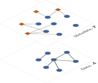
Figure 1: Schematic representation of the joint data-metadata model. The data layer is composed of data nodes and is described by an adjacency matrix $\bm{A}$, and the metadata layer is composed of the same data nodes, as well as tag nodes, and is described by a bipartite adjacency matrix $\bm{T}$. Both layers are generated by two coupled degree-corrected SBMs, where the partition of the data nodes into groups is the same in both layers.

We construct a generative model for the matrices $\bm{A}$ and $\bm{T}$ by generalizing the hierarchical stochastic block model (SBM) Peixoto (2014a) with degree-correction Karrer and Newman (2011) for the case with edge layers Peixoto (2015a). In this model, the nodes and tags are divided into $B_{d}$ and $B_{t}$ groups, respectively. The number of edges between data groups $r$ and $s$ are given by the parameters $e_{rs}$ (or twice that for $r=s$), and between data group $r$ and tag group $u$ by $m_{ru}$. Both data and tag nodes possess fixed degree sequences, $\{k_{i}\}$ and $\{d_{i}\}$, for the data and metadata layers, respectively, corresponding to an additional set of parameters. Given these constraints, a graph is generated by placing the edges randomly in both layers independently, with a joint likelihood

$$P(\bm{A},\bm{T}|\bm{b},\theta,\bm{c},\gamma)=P(\bm{A}|\bm{b},\theta)P(\bm{T}|\bm{b},\bm{c},\gamma),$$ (1)

where $\bm{b}=\{b_{i}\}$ and $\bm{c}=\{c_{i}\}$ are the group memberships of the data and tag nodes, respectively, and both $\theta=(\{e_{rs}\},\{k_{i}\})$ and $\gamma=(\{m_{ru}\},\{d_{i}\})$ are shorthands for the remaining model parameters in both layers. Inside each layer, the log-likelihood is Karrer and Newman (2011); Peixoto (2012)

$$\ln P(\bm{A}|\bm{b},\theta)\approx-E-\frac{1}{2}\sum_{rs}e_{rs}\ln\frac{e_{rs}}{e_{r}e_{s}}-\sum_{i}\ln k_{i}!,$$ (2)

and analogously for $P(\bm{T}|\bm{b},\bm{c},\gamma)$. Since the data nodes have the same group memberships in both layers, this provides a coupling between them, and we have thus a joint model for data and metadata. This model is general, since it is able to account simultaneously for the situation where there is a perfect correspondence between data and metadata (for example, when $B_{d}=B_{t}$ and the matrix $m_{ru}$ connects one data group to only one metadata group), when the correspondence is non-existent (the matrix $\bm{T}$ is completely random, with $B_{t}=1$), as well as any elaborate relationship between data and metadata in between. In principle, we could fit the above model by finding the model parameters that maximize the likelihood in Eq. 1. Doing so would uncover the precise relationship between data and metadata under the very general assumptions taken here. However, for this approach to work, we need to know a priori the number of groups $B_{d}$ and $B_{t}$. This is because the likelihood of Eq. 1 is parametric (i.e. it depends on the particular choices of $\bm{b}$, $\bm{c}$, $\theta$ and $\gamma$), and the degrees of freedom in the model will increase with $B_{d}$ and $B_{t}$. As the degrees of freedom increase, so will the likelihood, and the perceived quality of fit of the model. If we follow this criterion blindly, we will put each node and metadata tag in their individual groups, and our matrices $e_{rs}$ and $m_{rs}$ will correspond exactly to the adjacency matrices $\bm{A}$ and $\bm{T}$, respectively. This is an extreme case of overfitting, where we are not able to differentiate random fluctuations in data from actual structure that should be described by the model. The proper way to proceed in this situation is to make the model nonparametric, by including noninformative Bayesian priors on the model parameters $P(\bm{b})$, $P(\bm{c})$, $P(\theta)$ and $P(\gamma)$, as described in Ref. Peixoto (2014a, 2015b) (See also Appendix A). By maximizing the joint nonparametric likelihood $P(\bm{A},\bm{T},\bm{b},\theta,\bm{c},\gamma)=P(\bm{A},\bm{T}|\bm{b},\theta,\bm{c},\gamma)P(\bm{b})P(\theta)P(\bm{c})P(\gamma)$ we can find the best partition of the nodes and tags into groups, together with the number of groups themselves, without overfitting. This happens because, in this setting, the degrees of freedom of the model are themselves sampled from a distribution, which will intrinsically ascribe higher probabilities to simpler models, effectively working as a penalty on more complex ones. An equivalent way of justifying this is to observe that the joint likelihood can be expressed as $P(\bm{A},\bm{T},\bm{b},\theta,\bm{c},\gamma)=2^{-\Sigma}$, where $\Sigma$ is the description length of the data, corresponding to the number of bits necessary to encode both the data according to the model parameters as well as the model parameters themselves. Hence, maximizing the joint Bayesian likelihood is identical to the minimum description length (MDL) criterion Grünwald (2007); Rosvall and Bergstrom (2007), which is a formalization of Occam’s razor, where the simplest hypothesis is selected according to the statistical evidence available.

We note that there are some caveats when selecting the priors probabilities above. In the absence of a priori knowledge, the most straightforward approach is to select flat priors that encode this, and ascribe the same probability to all possible model parameters Jaynes (2003). This choice, however, incurs some limitations. In particular, it can be shown that with flat priors it is not possible to infer with the SBM a number of groups that exceeds an upper threshold that scales with $B_{\text{max}}\sim\sqrt{N}$, where $N$ is the number of nodes in the network Peixoto (2013). Additionally, flat priors are unlikely to be good models for real data, since they assume all parameters values are equally likely. This is an extreme form of randomness that encodes maximal ignorance about the model parameters. However no data is truly sampled from such a maximally random distribution; they are more likely to be sampled from some nonrandom distribution, but with an unknown shape. An alternative, therefore, is to postpone the decision on the prior until we observe the data, by sampling the prior distribution itself from a hyperprior. Of course, in doing so, we face the same problem again when selecting the hyperprior. For the model at hand, we proceed in the following manner: Since the matrices $\{e_{rs}\}$ and $\{m_{rs}\}$ are themselves adjacency matrices of multigraphs (with $B_{d}$ and $B_{d}+B_{t}$ nodes, respectively), we sample them from another set of SBMs, and so on, following a nested hierarchy, until the trivial model with $B_{d}=B_{t}=1$ is reached, as described in Ref. Peixoto (2014a). For the remaining model parameters we select only two-level Bayesian hierarchies, since it can be shown that higher-level ones have only negligible improvements asymptotically Peixoto (2015b). We review and summarize the prior probabilities in Appendix. A. With this Bayesian hierarchical model, not only we significantly increase the resolution limit to $B_{\text{max}}\sim N/\ln N$ Peixoto (2014a), but also we are able to provide a description of the data at multiple scales.

It is important to emphasize that we are not restricting ourselves to purely assortative structures, as it is the case in most community detection literature, but rather we are open to a much wider range of connectivity patterns that can be captured by the SBM. As mentioned in the introduction, our approach differs from the parametric model recently introduced by Newman and Clauset Newman and Clauset (2016), where it is assumed that a node can connect to only one metadata tag, and each tag is parametrized individually. In our model, a data node can possess zero, one or more annotations, and the tags are clustered into groups. Therefore our approach is suitable for a wider range of data annotations, where entire classes of metadata tags can be identified. Furthermore, since their approach is parametric, the appropriate number of groups must be known beforehand, instead of being obtained from data, which is seldom possible in practice. Additionally, when employing the fast MCMC algorithm developed in Ref. Peixoto (2014b), the inference procedure scales linearly as $O(N)$ (or log-linearly $O(N\ln^{2}N)$ when obtaining the full hierarchy Peixoto (2014a)), where $N$ is the number of nodes in the network, independently of the number of groups, in contrast to the expectation-maximization with belief propagation of Ref. Newman and Clauset (2016), that scales as $O(B^{2}N)$, where $B$ is the number of groups being inferred. Hence, our method scales well not only for large networks, but also for arbitrarily large number of communities. An implementation of our method is freely available as part of the graph-tool library Peixoto (2014c) at http://graph-tool.skewed.de.

This joint approach of modelling the data and metadata allows us to understand in detail the extent to which network structure and annotations are correlated, in a manner that puts neither in advantage with respect to the other. Importantly, we do not interpret the individual tags as “ground truth” labels on the communities, and instead infer their relationships with the data communities from the entire data. Because the metadata tags themselves can be clustered into groups, we are able to assess both their individual and collective roles. For instance, if two tag nodes are assigned to the same group, this means that they are both similarly informative on the network structure, even if their target nodes are different. By following the inferred probabilities between tag and node groups, one obtains a detailed picture of their correspondence, that can deviate in principle (and often does in practice) from the commonly assumed one-to-one mapping Yang and Leskovec (2012a); Hric et al. (2014), but includes it as a special case.

Before going into the systematic analysis of empirical datasets, we illustrate the application of this approach with a simple example, corresponding to the network of American college football teams Girvan and Newman (2002), where the edges indicate that a game occurred between two teams in a given season. For this data it is also available to which “conferences” the teams belong. Since it is expected that teams in the same conference play each other more frequently, this is assumed to be an indicator for the network structure. If we fit the above model to this dataset, both the nodes (teams) and tags (conferences) are divided into $B_{d}=10$ and $B_{t}=10$ groups, respectively (Fig. 2). Some of the conferences correspond exactly to the inferred groups of teams, as one would expect. However other conferences are clustered together, in particular the independents, meaning that although they are collectively informative on the network structure, individually they do not serve as indicators of the network topology in a manner that can be conclusively distinguished from random fluctuations.

In Fig. 2 we used the conference assignments presented in Ref. Evans (2010), which are different from the original assignments in Ref. Girvan and Newman (2002), due to a mistake in the original publication, where the information from the wrong season was used instead Evans (2012). We use this as an opportunity to show how errors and noise in the metadata can be assessed with our method, while at the same time we emphasize an important application, namely the prediction of missing nodes. We describe it in general terms, and then return to our illustration afterwards.

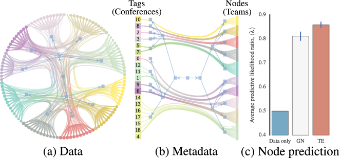
Figure 2: Joint data-metadata model inferred for the network of American football teams Girvan and Newman (2002). (a) Hierarchical partition of the data nodes (teams), corresponding to the “data” layer. (b) Partition of the data (teams) and tag (conference) nodes, corresponding to the second layer. (c) Average predictive likelihood of missing nodes relative to using only the data (discarding the conferences), using the original conference assignment of Ref. Girvan and Newman (2002) (GN) and the corrected assignment of Ref. Evans (2010) (TE).

II.1 Prediction of missing nodes

To predict missing nodes, we must compute the likelihood of all edges incident on it simultaneously, i.e. for an unobserved node $i$ they correspond to the $i$th row of the augmented adjacency matrix, $\bm{a}_{i}=\{A_{ij}^{\prime}\}$, with $A_{kj}^{\prime}=A_{kj}$ for $k\neq i$. If we know the group membership $b_{i}$ of the unobserved node, in addition to the observed nodes, the likelihood of the missing incident edges is

$$P(\bm{a}_{i}|\bm{A},b_{i},\bm{b}) =\frac{\sum_{\theta}P(\bm{A},\bm{a}_{i}|b_{i},\bm{b},\theta)P(\theta)}{\sum_{\theta}P(\bm{A}|\bm{b},\theta)P(\theta)}$$ (3)

$$=\frac{P(\bm{A},\bm{a}_{i}|b_{i},\bm{b},\hat{\theta})P(\hat{\theta})}{P(\bm{A}|\bm{b},\hat{\theta}^{\prime})P(\hat{\theta}^{\prime})},$$ (4)

where $\hat{\theta}$ and $\hat{\theta}^{\prime}$ are the only choices of parameters compatible with the node partition. However, we do not know a priori to which group the missing node belongs. If we have only the network data available (not the metadata) the only choice we have is to make the probability conditioned on the observed partition,

$$P(\bm{a}_{i}|\bm{A},\bm{b})=\sum_{b_{i}}P(\bm{a}_{i}|\bm{A},b_{i},\bm{b})P(b_{i}|\bm{b}),$$ (5)

where $P(b_{i}|\bm{b})=P(\bm{b},b_{i})/P(\bm{b})$. This means that we can use only the distribution of group sizes to guide the placement of the missing node, and nothing more. However, in practical scenarios we may have access to the metadata associated with the missing node. For example, in a social network we might know the social and geographical indicators (age, sex, country, etc) of a person for whom we would like to predict unknown acquaintances. In our model, this translates to knowing the corresponding edges in the tag-node graph $\bm{T}$. In this case, we can compute the likelihood of the missing edges in the data graph as

$$P(\bm{a}_{i}|\bm{A},\bm{T},\bm{b},\bm{c})=\sum_{b_{i}}P(\bm{a}_{i}|\bm{A},b_{i},\bm{b})P(b_{i}|\bm{T},\bm{b},\bm{c}),$$ (6)

where the node membership distribution is weighted by the information available in the full tag-node graph,

$$P(b_{i}|\bm{T},\bm{b},\bm{c}) =\frac{P(b_{i},\bm{b}|\bm{T},\bm{c})}{P(\bm{b}|\bm{T},\bm{c})}$$ (7)

$$=\frac{\sum_{\gamma}P(\bm{T}|b_{i},\bm{b},\bm{c},\gamma)P(b_{i},\bm{b})P(\gamma)}{\sum_{b_{i}^{\prime}}\sum_{\gamma}P(\bm{T}|b_{i}^{\prime},\bm{b},\bm{c},\gamma)P(b_{i}^{\prime},\bm{b})P(\gamma)}$$ (8)

$$=\frac{P(\bm{T}|b_{i},\bm{b},\bm{c},\hat{\gamma})P(b_{i},\bm{b})P(\hat{\gamma})}{\sum_{b_{i}^{\prime}}P(\bm{T}|b_{i}^{\prime},\bm{b},\bm{c},\hat{\gamma}^{\prime})P(b_{i}^{\prime},\bm{b})P(\hat{\gamma}^{\prime})},$$ (9)

where again $\hat{\gamma}$ and $\hat{\gamma}^{\prime}$ are the only choices of parameters compatible with the partitions $\bm{c}$ and $\bm{b}$. If the metadata correlates well with the network structure, the above distribution should place the missing node with a larger likelihood in its correct group. In order to quantify the relative predictive improvement of the metadata information for node $i$, we compute the predictive likelihood ratio $\lambda_{i}\in[0,1]$,

$$\lambda_{i}=\frac{P(\bm{a}_{i}|\bm{A},\bm{T},\bm{b},\bm{c})}{P(\bm{a}_{i}|\bm{A},\bm{T},\bm{b},\bm{c})+P(\bm{a}_{i}|\bm{A},\bm{b})},$$ (10)

which should take on values $\lambda_{i}>1/2$ if the metadata improves the prediction task, or $\lambda_{i}<1/2$ if it deteriorates it. The latter can occur if the metadata misleads the placement of the node (we discuss below the circumstances where this can occur).

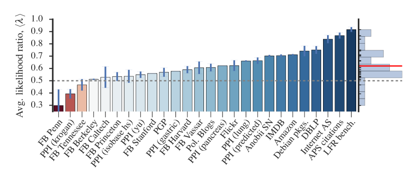
Figure 3: Node prediction performance, measured by the average predictive likelihood ratio ${\left<\lambda\right>}$ for a variety of annotated datasets (see Appendix B for descriptions). Values above $1/2$ indicate that the metadata improves the node prediction task. On the right axis a histogram of the likelihood ratios is shown, with a red line marking the average.

In order to illustrate this approach we return to the American football data, and compare the original and corrected conference assignments in their capacity of predicting missing nodes. We do so by removing a node from the network, inferring the model on the modified data, and computing its likelihood according to Eq. 5 and Eq. 7, which we use to compute the average predictive likelihood ratio for all nodes in the network, ${\left<\lambda\right>}=\sum_{i}\lambda_{i}/N$. As can be seen in Fig. 2c, including the metadata improves the prediction significantly, and indeed we observe that the corrected metadata noticeably improves the prediction when compared to the original inaccurate metadata. In short, knowing to which conference a football team belongs, does indeed increase our chances of predicting against which other teams it will play, and we may do so with a higher success rate using the current conference assignments, rather than using those of a previous year. These are hardly surprising facts in this illustrative context, but the situation becomes quickly less intuitive for datasets with hundreds of thousands of nodes and a comparable number of metadata tags, for which only automated methods such as ours can be relied upon.

III Empirical datasets

We performed a survey of several network datasets with metadata (described in detail in Appendix B), where we removed a small random fraction of annotated nodes ($1\%$ or $100$ nodes, whichever is smaller) many times, and computed the likelihood ratio $\lambda_{i}$ above for every removed node. The average value for each dataset is shown in Fig. 3. We observe that for the majority of datasets the metadata is capable of improving the prediction of missing nodes, with the quality of the improvement being relatively broadly distributed. While this means that there is a positive and statistically significant correlation between the metadata and the network structure, for some datasets this leads only to moderate predictive improvements. On the other hand, there is a minority of cases where the inclusion of metadata worsens the prediction task, leading to ${\left<\lambda\right>}<1/2$. In such situations, the metadata seems to divide the network in a manner that is largely orthogonal to the how the network itself is connected. In order to illustrate this, we consider some artificially generated datasets as follows, before returning to the empirical datasets.

III.1 Alignment between data and metadata

We construct a network with $N$ nodes divided into $B_{d}$ equal-sized groups, that are perfectly assortative, i.e. nodes of one group are only connected to other nodes of the same group. Furthermore, the $E$ edges of the network are randomly distributed among the groups, so that they have on average the same edge density. This yields a simple structure composed of the union of $B_{d}$ disjoint, fully random networks of similar density.

In the metadata layer we have the same number of $M=N$ metadata tags, which are themselves also divided into an equal number $B_{t}=B_{d}=B$ of equal-sized groups.

In order to place $E_{m}=E$ edges between data and metadata, we also consider an alternative partition $\{b^{\prime}_{i}\}$ of the data nodes into $B$ groups that is not equal to the original partition $\{b_{i}\}$ used to construct the network. A tag in one metadata group can only connect randomly to nodes of one particular data group, and vice versa. I.e. there is a one-to-one mapping between tag and data groups.

In total we consider three ways to connect the data with the metadata:

1. Aligned with the original data partition $\{b_{i}\}$, i.e. tag-node edges connect to the same data groups used to place the node-node edges;

2. Misaligned with the data partition, i.e. tag-node edges connect to the groups of the alternative data partition $\{b^{\prime}_{i}\}$;

3. Random: The tag-node edges are placed entirely at random, i.e. respecting neither the tag nor the node partitions.

We emphasize that 2 (misaligned) and 3 (random) are different: the former corresponds to structured metadata that is uncorrelated with the network structure, and the latter corresponds to unstructured metadata. In other words, in the misaligned case the node-tag graph is not fully random, since it only connects specific tag groups to specific node groups, whereas in the random case the node-tag edges are indeed fully random. An example of each type of construction for $B=2$ is shown in Fig. 4.

When performing node prediction for artificial networks constructed in this manner, one observes improved prediction with aligned metadata systematically; however with misaligned metadata a measurable degradation can be seen, while for random metadata neutral values close to ${\left<\lambda\right>}=1/2$ are observed (see Fig. 4). The degradation observed for misaligned metadata is due to the subdivision of the data groups into $B$ smaller subgroups, according to how they are connected to the metadata tags. This subdivision, however, is not a meaningful way of capturing the pattern of the node-node connections, since all nodes that belong to the same planted group are statistically indistinguishable. If the number of subgroups is sufficiently large, this will invariably induce the incorporation of noise into the model via the different number of edges incident on each subgroup. Since these differences result only from statistical fluctuations, they are bad predictors of unobserved data, and hence cause the degradation in predictive quality. We note, however, that in the limiting case where the number of nodes inside each subdivision becomes sufficiently large, the degradation vanishes, since these statistical fluctuations become increasingly less relevant (see Fig. 4, curve $N/B=10^{3}$). Nevertheless, for sufficiently misaligned metadata the total number of inferred data groups can increase significantly as $B_{d}=B_{d}^{0}\times B_{t}$, where $B_{d}^{0}$ is the number of data groups used to generate the network. Therefore, in practical scenarios, the presence of structured (i.e. non-random) metadata that is strongly uncorrelated with the network structure can indeed deteriorate node prediction, as observed in a few of the empirical examples shown in Fig. 3.

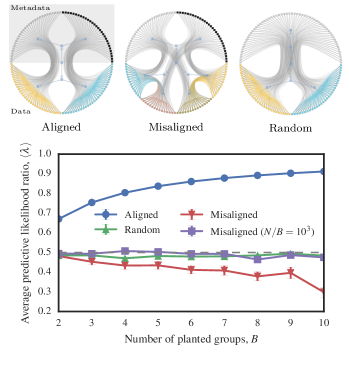
Figure 4: Top: Examples of artificial annotated networks, showing aligned, misaligned and random metadata, as described in the text. Bottom: Node prediction performance, measured by the likelihood ratio ${\left<\lambda\right>}$, average over all possible single-node removals, for annotated networks generated with $B_{d}=B_{t}=B$ groups, $N=M=30\times B$ nodes and tags, $E=E_{m}=5\times N$ node-node and tag-node edges, with specific network construction given by the legend. One of the curves corresponds to networks with misaligned metadata with a larger number of nodes, $N=M=10^{3}\times B$.

III.2 How informative are individual tags?

The average likelihood ratio ${\left<\lambda\right>}$ used above is measured by removing nodes from the network, and include the simultaneous contribution of all metadata tags that annotate them. However our model also divides the metadata tags into classes, which allows us to identify the predictiveness of each tag individually according to this classification. With this, one can separate informative from noninformative tags within a single dataset.

We again quantify the predictiveness of a metadata tag in its capacity to predict which other nodes will connect to the one it annotates. According to our model, the probability of some data node $i$ being annotated by tag $t$ is given by

$$P_{m}^{t}(i|t)=d_{i}\frac{m_{b_{i},c_{t}}}{m_{b_{i}}m_{c_{t}}},$$ (11)

which is conditioned on the group memberships of both data and metadata nodes. Analogously, the probability of some data node $i$ being a neighbor of a chosen data node $j$ is given by

$$P_{e}(i|j)=k_{i}\frac{e_{b_{i},b_{j}}}{e_{b_{i}}e_{b_{j}}}.$$ (12)

Hence, the probability of $i$ being a neighbor of any node $j$ that is annotated with tag $t$ is given by

$$P_{t}(i)=\sum_{j}P(i|j)P_{m}(j|t).$$ (13)

In order to compare the predictive quality of this distribution, we need to compare it to a null distribution where the tags connect randomly to the nodes,

$$Q(i)=\sum_{j}P(i|j)\Pi(j),$$ (14)

where $\Pi(i)=d_{i}/M$, with $M=\sum_{r<s}m_{rs}$, is the probability that node $i$ is annotated with any tag at random. The information gain obtained with the annotation is then quantified by the Kullback-Leibler divergence between both distributions,

$$D_{\text{KL}}(P_{t}||Q)=\sum_{i}P_{t}(i)\ln\frac{P_{t}(i)}{Q(i)}.$$ (15)

This quantity measures the amount of information lost when we use the random distribution $Q$ instead of the metadata-informed $P_{t}$ to characterize possible neighbors, and hence the amount we gain when we do the opposite. It is a strictly positive quantity, that can take any value between zero and $-\ln Q^{*}$, where $Q^{*}$ is the smallest non-zero value of $Q(i)$. If we substitute Eqs. 12 and 11 in Eq. 15, we notice that it only depends on the group membership of $t$, and can be written as

$$D_{\text{KL}}(P_{t}||Q)=D_{\text{KL}}(p_{c_{t}}||q)$$ (16)

with

$$p_{r}(u)=\sum_{s}p_{e}(u|s)p_{m}(s|u),\quad q(u)=\sum_{s}p_{e}(u|s)\pi(s),$$ (17)

being the probabilities of a node that belongs to group $u$ being a neighbor of a node annotated by a tag belonging to group $r$, for both the structured and random cases, where $p_{e}(u|s)=e_{us}/e_{s}$, $p_{m}(s|u)=m_{sr}/m_{r}$, and $\pi(s)=m_{s}/M$. Since this can take any value between zero and $-\ln q^{*}$, where $q^{*}$ is the smallest non-zero value of $q(u)$, this will in general depend on how many edges there are in the network, given that $q^{*}\geq 1/2E$. For a concise comparison between datasets of different sizes, it is useful to consider a relative version of this measure that does not depend on the size. Although one option is to normalize by the maximum possible value, here we use instead the entropy of $q$, $H(q)=-\sum_{r}q(r)\ln q(r)$, and denote the predictiveness $\mu_{r}$ of tag group $r$ as

$$\mu_{r}\equiv\frac{D_{\text{KL}}(p_{r}||q)}{H(q)}.$$ (18)

This gives us the relative improvement of the annotated prediction with respect to the uniformed one. Although it is possible to have $\mu_{r}>1$, this is not typical even for highly informative tags, and would mean that a particularly unlikely set of neighbors becomes particularly likely once we consider the annotation. Instead, a more typical highly informative metadata annotation simply narrows down the predicted neighborhood to a typical group sampled from $q$.

Using the above criterion we investigated in detail the datasets of Fig. 3, and quantified the predictiveness of the node annotations, as is shown in Fig. 5 for a selected subset. Overall, we observe that the datasets differ greatly not only in the overall predictiveness of their annotations, but also in the internal structures. Typically, we find that within a single dataset the metadata predictiveness is widely distributed. A good example of this is the IMDB data, which describes the connection between actors and films, and includes annotations on the films corresponding to the year and country of production, the producers, the production company, the genres, user ratings as well as user-contributed keywords. In Fig. 5a we see that the larger fraction of annotations posses very low predictiveness (which includes the vast majority of user-contributed keywords and ratings), however there is still a significant number of annotations that can be quite predictive. The most predictive types of metadata are combinations of producers and directors (e.g. Cartoon productions), followed by specific countries (e. g. New Zealand, Norway) and year of productions. Besides keywords and ratings, film genres are among those with the lowest predictiveness. A somewhat narrower variability is observed for the APS citation data in Fig. 5b, where the three types of annotations are clearly distinct. The PACS numbers are the most informative on average, followed by the date of publication (with older dates being more predictive then new ones — presumably due to the increasing publication volume and diversification over the years), and lastly the journal. One prominent exception is the most predictive metadata group that corresponds to the now-extinct “Physical Review (Series I)” journal, and its publication dates ranging from 1893 to 1913. For the Amazon dataset of Fig. 5c, the metadata also exhibits significant predictive variance, but there are no groups of tags that possess very low values, indicating that most product categories are indeed strong indications of co-purchases. This is similar to what is observed for the Internet AS, with most countries being good predictors of the network structure. The least predictive annotations happen to be a group of ten countries that include the US as the most frequent one. A much wider variance is observed in the DBLP collaboration network, where the publication venues seem to be divided in two branches: very frequent and popular ones with low to moderate predictiveness, and many very infrequent ones with high to very high predictiveness. For other datasets a wide variance in predictiveness is not observed. In particular for most Facebook networks as well as protein-protein interaction networks, the available metadata seems to be only tenuously correlated with the network structure, with narrowly-distributed values of low predictiveness, in accordance with their relatively low placement in Fig. 3.

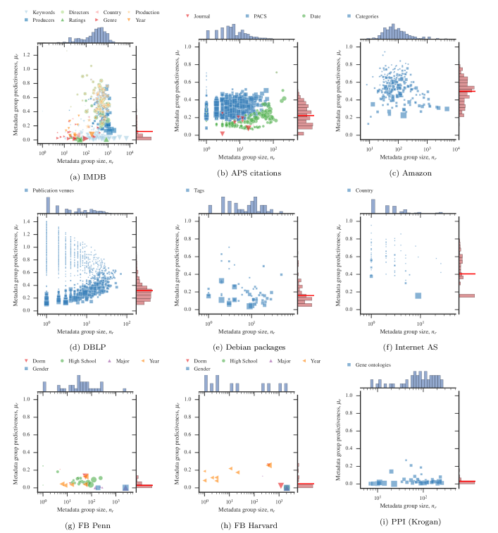
Figure 5: Metadata predictiveness for several empirical datasets. The figures show the predictiveness of metadata groups $\mu_{r}$ (Eq. 18) vs. metadata group sizes, $n_{r}$.The sizes of the symbols indicate the metadata frequency. The symbols correspond to the most frequent types of tags in each group (which may contain tags of different types). On the axis of each figure are shown marginal histograms, weighted according to the tag frequencies. A red horizontal line marks the average predictiveness.

IV Prediction of missing metadata

Since we have defined a full joint model for data and metadata, our framework is not restricted to prediction of missing nodes, but can also predict missing edges both in the data and metadata layers. The latter can be used to predict incomplete metadata information, which corresponds to missing edges between data nodes and metadata tags, as follows. Suppose the tag layer is decomposed as the union of two edge sets, $\delta\bm{T}\cup\bm{T}$, where $\bm{T}$ is a set of observed data-metadata edges, and $\delta\bm{T}$ is a set of missing edges of the same type. Under our model, we can write the marginal posterior likelihood for $\delta\bm{T}$ as

$$P(\delta\bm{T}|\bm{T},b,c)=\frac{P(\delta\bm{T}\cup\bm{T}|\bm{T},b,c)}{P(\bm{T}|b,c)},$$ (19)

where $P(\bm{T}|b,c)=\sum_{\delta\bm{T}}P(\delta\bm{T}\cup\bm{T}|b,c)$ is a normalization constant. If we have our set of missing edges coming from a restricted set of possibilities, $\delta\bm{T}\in\{\delta\bm{T}_{1},\delta\bm{T}_{2},\dots\}$, we may write the predictive likelihood ratio

$$\lambda_{i}=\frac{P(\delta\bm{T}_{i}|\bm{T},b,c)}{\sum_{j}P(\delta\bm{T}_{j}|\bm{T},b,c)}=\frac{P(\delta\bm{T}_{i}\cup\bm{T}|b,c)}{\sum_{j}P(\delta\bm{T}_{j}\cup\bm{T}|b,c)},$$ (20)

where the normalization constant of Eq. 19 no longer plays a role. Hence, if we want to compare the likelihood of a given set of alternative node annotations, all we need to do is to infer the parameters $b$ and $c$ of the model given the observed network,

$$\{\hat{b},\hat{c}\}=\underset{\{b,c\}}{\operatorname{argmax}}\;P(\bm{T}|b,c)P(b)P(c),$$ (21)

and then add the missing edges $\delta\bm{T}_{i}$ to the likelihood using this parameter estimate to compute the likelihood ratio of Eq. 20.

We illustrate the application of our method again with the American college football data. For each data node (team), we remove the single metadata tag associated with it (i.e. the team’s conference), perform the model inference, and compute the predictive likelihood ratio of Eq. 20 for the removed tag, with respect to all other possible tags. The averages over all teams that belong to a given conference are shown in Fig. 6. The method succeeds in predicting the correct conference assignment with the highest likelihood in all cases, except for the “independent” teams. These teams do not belong to any conference, and are therefore assigned a unique conference tag. When this assignment is removed, it leaves an independent tag without any connection to the graph, and hence out model is not able to predict its placement. But since there is no additional information in the data once this sole assignment is removed, it is simply impossible to make an informative guess. In the cases where it is possible, our approach seems able to leverage the available information and increases the changes of successful metadata prediction.

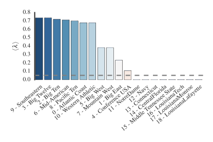
Figure 6: Average predictive likelihood ratio ${\left<\lambda\right>}$ of missing metadata tags (conferences) for the American football data, using the annotations given in Ref. Evans (2012). Tags $11$ to $18$ are “independents”, i.e. teams that do not belong to any conference. The dashed line marks the value $1/19$, corresponding to a uniform likelihood between all tags.

V Conclusion

We presented a general model for the large-scale structure of annotated networks that does not intrinsically assume that there is a direct correspondence between metadata tags and the division of network into groups, or communities. Instead, we assume that the data-metadata correlation is itself generated by an underlying process, with parameters that are unknown a priori. We presented a Bayesian framework to infer the model parameters from data, which is capable of uncovering — in addition to the network structure — the connection between network structure and annotations, if there is one to be found. We showed how this information can be used to predict missing nodes in the network when only the annotations are known.

When applying the method for a variety of annotated datasets, we found that their annotations lie in a broad range with respect to their correlation with network structure. For most datasets considered, there is evidence for statistically significant correlations between the annotations and the network structure, in a manner that can be detected by our method, and exploited for the task of node prediction. For a few datasets, however, we found evidence of metadata which is not trivially structured, but seems to be largely uncorrelated with the actual network structure.

The predictiveness variance of metadata observed across different datasets is also often found inside individual datasets. Typically, single datasets possess a wealth of annotations, most of which are not very informative on the network structure, but a smaller fraction clearly is. Our method is capable of separating groups of annotations with respect to their predictiveness, and hence can be used to prune such datasets from “metadata noise”, by excluding low-performing tags from further analysis.

As is always true when doing statistical inference, results obtained are conditioned on the validity of the model formulation, which invariably includes assumptions about the data-generating process. In our case, this means that the data-metadata layer can be represented as a graph, and that it is well modelled by a SBM. Naturally, this is only one of many possibilities, and it remains an open problem to determine which alternatives work best for any given annotated network. This is particularly true for annotations that correspond to continuous values (e.g. time and space), which would need either to be discretized before the application of our method, or preferably, would require a different modelling ansatz (see e.g. Ref. Newman and Clauset (2016)).

Nevertheless, we argue that the present approach is an appropriate starting point, that provides an important but overlooked perspective in the context of community detection validation. In a recent study Hric et al. (2014) a systematic comparison between various community detection methods and node annotations was performed, where for most of them strong discrepancies were observed. If we temporarily (and unjustifiably) assume a direct agreement with available annotations as the “gold standard”, this discrepancy can be interpreted in a few ways. Firstly, the methods might be designed to find structures that fit the data poorly, and hence cannot capture their most essential features. Secondly, even if the general ansatz is sound, a given algorithm might still fail for more technical and subtle reasons. For example, most methods considered in Ref. Hric et al. (2014) do not attempt to gauge the statistical significance of their results, and hence are subject to overfitting Guimerà et al. (2004); Good et al. (2010). This incorporation of statistical noise will result in largely meaningless division of the networks, which would be poorly correlated with the “true” division. Additionally, recently Newman and Clauset Newman and Clauset (2016) suggested that while the best-fitting division of the network can be poorly correlated with the metadata, the network may still admit alternative divisions that are also statistically significant, but happen to be well correlated with the annotations.

On the other hand, the metadata heterogeneity we found with our method gives a strong indication that node annotations should not be used in direct comparisons to community detection methods in the first place — at least not indiscriminately. In most networks we analyzed, even when the metadata is strongly predictive of the network structure, the agreement between the annotations and the network division tends to be complex, and very different from the one-to-one mapping that is more commonly assumed. Furthermore, almost all datasets contain considerable noise in their annotations, corresponding to metadata tags that are essentially random. From this, we argue that data annotations should not be used as a panacea in the validation of community detection methods. Instead, one should focus on validation methods that are grounded in statistical principles, and use the metadata as source of additional evidence — itself possessing its own internal structures and also subject to noise, errors and omissions — rather than a form of absolute truth.

Appendix A Model likelihood and priors

As mentioned in the text, the microcanonical degree-corrected SBM log-likelihood is given by Peixoto (2012)

$$\ln P(\bm{A}|\bm{b},\theta)\approx-E-\frac{1}{2}\sum_{rs}e_{rs}\ln\frac{e_{rs}}{e_{r}e_{s}}-\sum_{i}\ln k_{i}!,$$ (22)

(if Stirling’s factorial approximation is used) and likewise for $\ln P(\bm{T}|\bm{c},\gamma)$, where one replaces $e_{rs}$ by $m_{rs}$ and $k_{i}$ by $d_{i}$,

$$\ln P(\bm{T}|\bm{c},\gamma)\approx-M-\frac{1}{2}\sum_{rs}m_{rs}\ln\frac{m_{rs}}{m_{r}m_{s}}-\sum_{i}\ln d_{i}!,$$ (23)

where $E=\sum_{rs}e_{rs}/2$ and $M=\sum_{rs}m_{rs}/2$. This assumes that the graph is sufficiently sparse, otherwise corrections need to be introduced, as described in Ref. Peixoto (2012, 2015b). In order to compute the full joint likelihood, we need priors for the parameters $\{b_{i}\}$, $\{c_{i}\}$, $\{k_{i}\}$, $\{d_{i}\}$, $\{e_{rs}\}$ and $\{m_{rs}\}$.

For the node partitions, we use a two-level Bayesian hierarchy as done in Ref. Peixoto (2014a), where one first samples the group sizes from a random histogram, and then the node partition randomly conditioned on the group sizes. The nonparametric likelihood is given by $P(\{b_{i}\})=e^{-\mathcal{L}_{p}}$, with

$$\mathcal{L}_{p}=\ln{\textstyle\left(\kern-3.00003pt\left(\genfrac{}{}{0.0pt}{}{B}{N}\right)\kern-3.00003pt\right)}+\ln N!-\sum_{r}\ln n_{r}!,$$ (24)

where $\left(\kern-3.00003pt\left(\genfrac{}{}{0.0pt}{}{n}{m}\right)\kern-3.00003pt\right)={n+m-1\choose m}$ is the total number of $m$-combinations with repetitions from a set of size $n$. The prior $P(\{c_{i}\})$ is analogous.

For the degree sequences, we proceed in the same fashion Peixoto (2015b), by sampling the degrees conditioned on the total number of edges incident on each group, by first sampling a random degree histogram with a fixed average, and finally the degree sequence conditioned on this distribution. This leads to a likelihood $P(\{k_{i}\}|\{e_{rs}\},\{b_{i}\})=e^{-\mathcal{L}_{\kappa}}$, with

$$\mathcal{L}_{\kappa}=\sum_{r}\ln\Xi_{r}+\ln n_{r}!-\sum_{k}\ln n^{r}_{k}!,$$ (25)

where $\ln\Xi_{r}\simeq 2\sqrt{\zeta(2)e_{r}}$. Again, the likelihood for $P(\{d_{i}\}|\{m_{rs}\},\{c_{i}\})$ is entirely analogous.

For the matrix of edge counts $\{e_{rs}\}$ we use the hierarchical prior proposed in Ref. Peixoto (2014a). Here we view this matrix as the adjacency matrix of a multigraph with $B_{d}$ nodes and $E_{d}=\sum_{rs}e_{rs}/2$ edges. We sample this multigraph from another SBM with a number of groups $B_{d}^{1}$, which itself is sampled from another SBM with $B_{d}^{2}$ groups and so on, until $B_{d}^{L}=1$ for some depth $L$. The whole nonparametric likelihood is then $P(\{e_{rs}\})=e^{-\Sigma}$, with

$$\Sigma=\sum_{l=1}^{L}S_{m}(\{e^{l}_{rs}\},\{n^{l}_{r}\})+\mathcal{L}^{l-1}_{t},$$ (26)

with $\{e^{l}_{rs}\}$, $\{n^{l}_{r}\}$ describing the block model at level $l$, and

$$\mathcal{S}_{m}=\sum_{r>s}\ln{\textstyle\left(\kern-3.00003pt\left(\genfrac{}{}{0.0pt}{}{n_{r}n_{s}}{e_{rs}}\right)\kern-3.00003pt\right)}+\sum_{r}\ln{\textstyle\left(\kern-3.00003pt\left(\genfrac{}{}{0.0pt}{}{\left(\kern-2.10002pt\left(\genfrac{}{}{0.0pt}{}{n_{r}}{2}\right)\kern-2.10002pt\right)}{e_{rr}/2}\right)\kern-3.00003pt\right)}$$ (27)

is the entropy of the corresponding multigraph ensemble and

$$\mathcal{L}^{l}_{t}=\ln{\textstyle\left(\kern-3.00003pt\left(\genfrac{}{}{0.0pt}{}{B_{l}}{B_{l-1}}\right)\kern-3.00003pt\right)}+\ln B_{l-1}!-\sum_{r}\ln n_{r}^{l}!.$$ (28)

is the description length of the node partition at level $l>0$. The procedure is exactly the same for the prior $P(\{m_{rs}\})$.

Appendix B Datasets

Below we list descriptions of the annotated datasets used in this work. Basic statistics are given in Table 1.

Dataset	$N_{d}$	$E_{d}$	$N_{t}$	$E_{t}$	$B_{d}$	$B_{t}$
LFR	1,000	9,839	40	1,000	29	29
PPI (Krogan)	5,247	45,899	4,896	5,4904	62	55
PPI (Yu)	964	1,487	2,119	10,304	16	17
PPI (isobase-hs)	8,580	34,250	1,972	20,633	40	15
PPI (gastric)	4,763	26,131	10,445	94,035	50	50
PPI (lung)	4,843	27,459	10,948	100,492	55	50
PPI (pancreas)	4,759	25,978	10,444	93,686	49	46
PPI (predicted)	7,606	23,446	12,337	143,847	69	68
FB Caltech	762	16,651	591	4,145	22	5
FB Penn	41,536	1,362,220	4,805	216,349	365	29
FB Harvard	15,086	824,595	3,942	74,293	192	15
FB Stanford	11,586	568,309	3,337	57,940	182	12
FB Berkeley	22,900	852,419	2,906	116,556	267	16
FB Princeton	6,575	293,307	2,396	32,901	110	10
FB Tennessee	16,977	770,658	2,660	89,458	271	20
FB Vassar	3,068	119,161	1,620	16,859	69	12
Pol. blogs	1,222	16,714	2	1,222	12	2
DPD	35,029	161,313	580	115,999	253	59
PGP	39,796	197,150	35,370	148,966	485	380
Internet AS	46,676	262,953	225	45,987	224	59
aNobii	140,687	869,448	8,003	926,403	194	70
Amazon	366,997	987,942	43,807	1,775,085	4,477	255
DBLP	317,080	1,049,866	13,477	719,820	4,667	1,746
IMDB	372,787	1,812,657	139,025	3,030,003	843	328
APS citations	437,914	4,596,335	22,530	1,916,281	5,681	954
Flickr	1,624,992	15,476,836	99,270	8,493,666	779	158

Table 1: Summary of the basic statistics of the datasets used in this work. $N_{d}$ and $E_{d}$ are the number of data nodes and data-data edges, respectively, whereas $N_{t}$ and $E_{t}$ are the number of metadata tags and node-tag edges, respectively. $B_{d}$ and $B_{t}$ are the number of data and metadata groups inferred with our method.

LFR.

Lancichinetti-Fortunato-Radicchi benchmark graph with $N=1000$ vertices and community sizes between $10$ and $50$, with mixing parameter $\mu=0.5$ Lancichinetti et al. (2008). The remaining parameters are the same as in Ref. Lancichinetti et al. (2008). This model corresponds to a specific parametrization of the degree-corrected SBM Karrer and Newman (2011), and is often used to test and optimize most current algorithms, and thus serves as a baseline reference for a network with known and detectable structure. The network was created with standard LFR code available at https://sites.google.com/site/santofortunato/inthepress2.

PPI networks.

In these networks nodes are individual proteins, and there is a link between them if there is a confirmed interaction. Protein labels from Gene Ontology project (GO) are used as node annotations. The networks themselves correspond to several different sources: Krogan and Yu correspond to yeast (Saccharomyces Cerevisiae), from two different publications: Krogan Collins et al. (2007) and Yu Yu et al. (2008); isobase-hs corresponds to human proteins, as collected by the Isobase project Park et al. (2011); Predicted include predicted and experimentally determined protein-protein interactions for humans, from the PrePPI project Zhang et al. (2013) (human interactions that are in the HC reference set predicted by structural modeling but not non-structural clues); Gastric, pancreas, lung are obtained by splitting the PrePPI network Zhang et al. (2013) by the tissue where each protein is expressed.

Facebook networks (FB).

Networks of social connections on the facebook.com online social network, obtained in 2005, corresponding to students of different universities Traud et al. (2012). All friendships are present as undirected links, as well as six types of annotation: Dorm (residence hall), major, second major, graduation year, former high school, and gender.

Internet AS.

Network of the Internet at the level of Autonomous Systems (AS). Nodes represent autonomous systems, i.e. systems of connected routers under the control of one or more network operators with a common routing policy. Links represent observed paths of Internet Protocol traffic directly from one AS to another. The node annotations are countries of registration of each AS. The data were obtained from the CAIDA project.

DBLP.

Network of collaboration of computer scientists. Two scientists are connected if they have coauthored at least one paper Backstrom et al. (2006). Node annotations are publication venues (scientific conferences). Data is downloaded from SNAP Yang and Leskovec (2012a).

aNobii.

This is an online social network for sharing book recommendations, popular in Italy. Nodes are user profiles, and there can be two types of directed relationships between them, which we used as undirected links (“friends” and “neighbors”). Data were provided by Luca Aiello Aiello et al. (2012, 2010). We used all present node metadata, of which there are four kinds: Age, location, country, and membership.

PGP.

The “Web of trust” of PGP (Pretty Good Privacy) key signings, representing an indication of trust of the identity of one person (signee) by another (signer). A node represents one key, usually but not always corresponding to a real person or organization. Links are signatures, which by convention are intended to only be made if the two parties are physically present, have verified each others’ identities, and have verified the key fingerprints. Data is taken from a 2009 snapshot of public SKS keyservers Richters and Peixoto (2011).

Flickr.

Picture sharing web site and social network, as crawled by Mislove et al Mislove et al. (2007). Nodes are users and edges exist if one user “follows” another. The node annotations are user groups centered around a certain type of content, such as “nature” or “Finland”.

Political Blogs.

A directed network of hyperlinks between weblogs on US politics, recorded in 2005 by Adamic and Glance Adamic and Glance (2005). Links are all front-page hyperlinks at the time of the crawl. Node annotations are “liberal” or “conservative” as assigned by either blog directories or occasional self-evaluation.

Debian packages.

Software dependencies within the Debian GNU/Linux operating system. Nodes are unique software packages, such as linux-image-2.6-amd64, libreoffice-gtk, or python-scipy. Links are the “depends”, “recommends”, and “suggests” relationships, which are a feature of Debian’s APT package management system designed for tracking dependencies. Node annotations are tag memberships from the DebTags project, such as devel::lang:python or web::browser Zini (2005). The network was generated from package files in Debian 7.1 Wheezy as of 2013-07-15, “main” area only. Similar files are freely available in every Debian-based OS. Tags can be found in the *_Packages files in the /var/lib/apt/ directory in an installed system or on mirrors, for example ftp://ftp.debian.org/debian/dists/wheezy/main/binary-amd64/.

amazon.

Network of product copurchases on online retailer amazon.com. Nodes represent products, and edges are said to represent copurchases by other customers presented on the product page Leskovec et al. (2007). The true meaning of links is unknown and is some function of Amazon’s recommendation algorithm. Data was scraped in mid-2006 and downloaded from http://snap.stanford.edu/data/amazon-meta.html. We used copurchasing relationships as undirected edges. Product categories were used as node annotations. Although product categories are hierarchical by nature, we used only the endpoints (or “leaves”) of the hierarchy: Books/Fiction/Fantasy/Epic and Books/Nonfiction are two different metadata labels.

IMDB.

This network is compiled by extracting information available in the Internet Movie Database (IMDB), and it contains each cast member and film as distinct nodes, and an undirected edge exists between a film and each of its cast members. The network used here corresponds to a snapshot made in 2012 Peixoto (2013). The node annotations are the following information available on the films: Country and year of production, production company, producers, directors, genre, user-contributed keywords and genres.

APS citations.

This network corresponds to directed citations between papers published in journals of the American Physical Society for a period of over 100 years. The node annotations correspond to PACS classification tags, journal and publication date.

References

- Fortunato (2010) Santo Fortunato, “Community detection in graphs,” Physics Reports 486, 75–174 (2010).
- Porter et al. (2009) Mason A Porter, Jukka-Pekka Onnela, and Peter J Mucha, “Communities in Networks,” 0902.3788 (2009), notices of the American Mathematical Society, Vol. 56, No. 9: 1082-1097, 1164-1166, 2009.
- Newman (2011) M. E. J. Newman, “Communities, modules and large-scale structure in networks,” Nat Phys 8, 25–31 (2011).
- Yang and Leskovec (2012a) Jaewon Yang and Jure Leskovec, “Defining and evaluating network communities based on ground-truth,” in Proceedings of the ACM SIGKDD Workshop on Mining Data Semantics, MDS ’12 (ACM, New York, NY, USA, 2012) pp. 3:1–3:8.
- Yang and Leskovec (2012b) Jaewon Yang and J. Leskovec, “Community-Affiliation Graph Model for Overlapping Network Community Detection,” in 2012 IEEE 12th International Conference on Data Mining (ICDM) (2012) pp. 1170–1175.
- Yang and Leskovec (2012c) Jaewon Yang and Jure Leskovec, “Structure and Overlaps of Communities in Networks,” arXiv:1205.6228 [physics] (2012c), arXiv: 1205.6228.
- Hric et al. (2014) Darko Hric, Richard K. Darst, and Santo Fortunato, “Community detection in networks: structural clusters versus ground truth,” arXiv:1406.0146 [physics, q-bio] (2014), arXiv: 1406.0146.
- Peixoto (2015a) Tiago P. Peixoto, “Inferring the mesoscale structure of layered, edge-valued, and time-varying networks,” Phys. Rev. E 92, 042807 (2015a).
- Stanley et al. (2015) Natalie Stanley, Saray Shai, Dane Taylor, and Peter J. Mucha, “Clustering Network Layers With the Strata Multilayer Stochastic Block Model,” arXiv:1507.01826 [physics, stat] (2015), arXiv: 1507.01826.
- Aicher et al. (2015) Christopher Aicher, Abigail Z. Jacobs, and Aaron Clauset, “Learning latent block structure in weighted networks,” jcomplexnetw 3, 221–248 (2015).
- Vallès-Català et al. (2016) Toni Vallès-Català, Francesco A. Massucci, Roger Guimerà, and Marta Sales-Pardo, “Multilayer Stochastic Block Models Reveal the Multilayer Structure of Complex Networks,” Phys. Rev. X 6, 011036 (2016).
- Moore et al. (2011) Cristopher Moore, Xiaoran Yan, Yaojia Zhu, Jean-Baptiste Rouquier, and Terran Lane, “Active learning for node classification in assortative and disassortative networks,” in Proceedings of the 17th ACM SIGKDD international conference on Knowledge discovery and data mining, KDD ’11 (ACM, New York, NY, USA, 2011) pp. 841–849.
- Leng et al. (2013) Mingwei Leng, Yukai Yao, Jianjun Cheng, Weiming Lv, and Xiaoyun Chen, “Active Semi-supervised Community Detection Algorithm with Label Propagation,” in Database Systems for Advanced Applications, Lecture Notes in Computer Science No. 7826, edited by Weiyi Meng, Ling Feng, Stéphane Bressan, Werner Winiwarter, and Wei Song (Springer Berlin Heidelberg, 2013) pp. 324–338, dOI: 10.1007/978-3-642-37450-0_25.
- Peel (2015) Leto Peel, “Active discovery of network roles for predicting the classes of network nodes,” jcomplexnetw 3, 431–449 (2015).
- Yang et al. (2013) Jaewon Yang, J. McAuley, and J. Leskovec, “Community Detection in Networks with Node Attributes,” in 2013 IEEE 13th International Conference on Data Mining (ICDM) (2013) pp. 1151–1156.
- Bothorel et al. (2015) Cecile Bothorel, Juan David Cruz, Matteo Magnani, and Barbora Micenkova, “Clustering attributed graphs: models, measures and methods,” arXiv:1501.01676 [physics] (2015), arXiv: 1501.01676.
- Zhang et al. (2014) Pan Zhang, Cristopher Moore, and Lenka Zdeborová, “Phase transitions in semisupervised clustering of sparse networks,” Phys. Rev. E 90, 052802 (2014).
- Zhang (2013) Zhong-Yuan Zhang, “Community structure detection in complex networks with partial background information,” EPL 101, 48005 (2013).
- Freno et al. (2011) Antonino Freno, Gemma Garriga, and Mikaela Keller, “Learning to Recommend Links using Graph Structure and Node Content,” (2011).
- Newman and Clauset (2016) M. E. J. Newman and Aaron Clauset, “Structure and inference in annotated networks,” Nat Commun 7, 11863 (2016).
- Liben-Nowell and Kleinberg (2007) David Liben-Nowell and Jon Kleinberg, “The link-prediction problem for social networks,” Journal of the American Society for Information Science and Technology 58, 1019–1031 (2007).
- Clauset et al. (2008) Aaron Clauset, Cristopher Moore, and M. E. J. Newman, “Hierarchical structure and the prediction of missing links in networks,” Nature 453, 98–101 (2008).
- Guimerà and Sales-Pardo (2009) Roger Guimerà and Marta Sales-Pardo, “Missing and spurious interactions and the reconstruction of complex networks,” Proceedings of the National Academy of Sciences 106, 22073 –22078 (2009).
- Guimerà and Sales-Pardo (2013) Roger Guimerà and Marta Sales-Pardo, “A Network Inference Method for Large-Scale Unsupervised Identification of Novel Drug-Drug Interactions,” PLOS Comput Biol 9, e1003374 (2013).
- Rovira-Asenjo et al. (2013) Núria Rovira-Asenjo, Tània Gumí, Marta Sales-Pardo, and Roger Guimerà, “Predicting future conflict between team-members with parameter-free models of social networks,” Sci. Rep. 3 (2013), 10.1038/srep01999.
- Musmeci et al. (2013) Nicolò Musmeci, Stefano Battiston, Guido Caldarelli, Michelangelo Puliga, and Andrea Gabrielli, “Bootstrapping Topological Properties and Systemic Risk of Complex Networks Using the Fitness Model,” J Stat Phys 151, 720–734 (2013).
- Cimini et al. (2015) Giulio Cimini, Tiziano Squartini, Andrea Gabrielli, and Diego Garlaschelli, “Estimating topological properties of weighted networks from limited information,” Phys. Rev. E 92, 040802 (2015).
- Rossi et al. (2012) Ryan A. Rossi, Luke K. McDowell, David W. Aha, and Jennifer Neville, “Transforming Graph Data for Statistical Relational Learning,” J. Artif. Int. Res. 45, 363–441 (2012).
- Bringmann et al. (2010) B. Bringmann, M. Berlingerio, F. Bonchi, and A. Gionis, “Learning and Predicting the Evolution of Social Networks,” IEEE Intelligent Systems 25, 26–35 (2010).
- Kim and Leskovec (2011) M. Kim and J. Leskovec, “The Network Completion Problem: Inferring Missing Nodes and Edges in Networks,” in Proceedings of the 2011 SIAM International Conference on Data Mining, Proceedings (Society for Industrial and Applied Mathematics, 2011) pp. 47–58.
- Kivelä et al. (2014) Mikko Kivelä, Alex Arenas, Marc Barthelemy, James P. Gleeson, Yamir Moreno, and Mason A. Porter, “Multilayer networks,” jcomplexnetw 2, 203–271 (2014).
- De Domenico et al. (2013) Manlio De Domenico, Albert Solé-Ribalta, Emanuele Cozzo, Mikko Kivelä, Yamir Moreno, Mason A. Porter, Sergio Gómez, and Alex Arenas, “Mathematical Formulation of Multilayer Networks,” Phys. Rev. X 3, 041022 (2013).
- Peixoto (2014a) Tiago P. Peixoto, “Hierarchical Block Structures and High-Resolution Model Selection in Large Networks,” Phys. Rev. X 4, 011047 (2014a).
- Karrer and Newman (2011) Brian Karrer and M. E. J. Newman, “Stochastic blockmodels and community structure in networks,” Phys. Rev. E 83, 016107 (2011).
- Peixoto (2012) Tiago P. Peixoto, “Entropy of stochastic blockmodel ensembles,” Phys. Rev. E 85, 056122 (2012).
- Peixoto (2015b) Tiago P. Peixoto, “Model Selection and Hypothesis Testing for Large-Scale Network Models with Overlapping Groups,” Phys. Rev. X 5, 011033 (2015b).
- Grünwald (2007) Peter D. Grünwald, The Minimum Description Length Principle (The MIT Press, 2007).
- Rosvall and Bergstrom (2007) Martin Rosvall and Carl T. Bergstrom, “An information-theoretic framework for resolving community structure in complex networks,” PNAS 104, 7327–7331 (2007).
- Jaynes (2003) E. T. Jaynes, Probability Theory: The Logic of Science, edited by G. Larry Bretthorst (Cambridge University Press, Cambridge, UK ; New York, NY, 2003).
- Peixoto (2013) Tiago P. Peixoto, “Parsimonious Module Inference in Large Networks,” Phys. Rev. Lett. 110, 148701 (2013).
- Decelle et al. (2011) Aurelien Decelle, Florent Krzakala, Cristopher Moore, and Lenka Zdeborová, “Asymptotic analysis of the stochastic block model for modular networks and its algorithmic applications,” Phys. Rev. E 84, 066106 (2011).
- Peixoto (2014b) Tiago P. Peixoto, “Efficient Monte Carlo and greedy heuristic for the inference of stochastic block models,” Phys. Rev. E 89, 012804 (2014b).
- Peixoto (2014c) Tiago P. Peixoto, “The graph-tool python library,” figshare (2014c), 10.6084/m9.figshare.1164194.
- Girvan and Newman (2002) M. Girvan and M. E. J. Newman, “Community structure in social and biological networks,” Proceedings of the National Academy of Sciences 99, 7821 –7826 (2002).
- Evans (2010) T S Evans, “Clique graphs and overlapping communities,” Journal of Statistical Mechanics: Theory and Experiment 2010, P12037 (2010).
- Evans (2012) T S Evans, “American College Football Network Files,” FigShare (2012), 10.6084/m9.figshare.93179.
- Guimerà et al. (2004) Roger Guimerà, Marta Sales-Pardo, and Luís A. Nunes Amaral, “Modularity from fluctuations in random graphs and complex networks,” Phys. Rev. E 70, 025101 (2004).
- Good et al. (2010) Benjamin H. Good, Yves-Alexandre de Montjoye, and Aaron Clauset, “Performance of modularity maximization in practical contexts,” Phys. Rev. E 81, 046106 (2010).
- Lancichinetti et al. (2008) Andrea Lancichinetti, Santo Fortunato, and Filippo Radicchi, “Benchmark graphs for testing community detection algorithms,” Phys. Rev. E 78, 046110 (2008).
- Collins et al. (2007) Sean R. Collins, Patrick Kemmeren, Xue-Chu Zhao, Jack F. Greenblatt, Forrest Spencer, Frank C. P. Holstege, Jonathan S. Weissman, and Nevan J. Krogan, “Toward a comprehensive atlas of the physical interactome of Saccharomyces cerevisiae,” Mol. Cell Proteomics 6, 439–450 (2007).
- Yu et al. (2008) Haiyuan Yu, Pascal Braun, Muhammed A. Yildirim, Irma Lemmens, Kavitha Venkatesan, Julie Sahalie, Tomoko Hirozane-Kishikawa, Fana Gebreab, Na Li, Nicolas Simonis, Tong Hao, Jean-François Rual, Amélie Dricot, Alexei Vazquez, Ryan R. Murray, Christophe Simon, Leah Tardivo, Stanley Tam, Nenad Svrzikapa, Changyu Fan, Anne-Sophie de Smet, Adriana Motyl, Michael E. Hudson, Juyong Park, Xiaofeng Xin, Michael E. Cusick, Troy Moore, Charlie Boone, Michael Snyder, Frederick P. Roth, Albert-László Barabási, Jan Tavernier, David E. Hill, and Marc Vidal, “High-quality binary protein interaction map of the yeast interactome network,” Science 322, 104–110 (2008).
- Park et al. (2011) Daniel Park, Rohit Singh, Michael Baym, Chung-Shou Liao, and Bonnie Berger, “IsoBase: a database of functionally related proteins across PPI networks,” Nucleic Acids Res. 39, D295–300 (2011).
- Zhang et al. (2013) Qiangfeng Cliff Zhang, Donald Petrey, José Ignacio Garzón, Lei Deng, and Barry Honig, “PrePPI: a structure-informed database of protein-protein interactions,” Nucleic Acids Res. 41, D828–833 (2013).
- Traud et al. (2012) Amanda L. Traud, Peter J. Mucha, and Mason A. Porter, “Social structure of Facebook networks,” Physica A: Statistical Mechanics and its Applications 391, 4165–4180 (2012).
- Backstrom et al. (2006) Lars Backstrom, Dan Huttenlocher, Jon Kleinberg, and Xiangyang Lan, “Group Formation in Large Social Networks: Membership, Growth, and Evolution,” in Proceedings of the 12th ACM SIGKDD International Conference on Knowledge Discovery and Data Mining, KDD ’06 (ACM, New York, NY, USA, 2006) pp. 44–54.
- Aiello et al. (2012) Luca Maria Aiello, Martina Deplano, Rossano Schifanella, and Giancarlo Ruffo, “People Are Strange When You’re a Stranger: Impact and Influence of Bots on Social Networks,” in Sixth International AAAI Conference on Weblogs and Social Media (2012).
- Aiello et al. (2010) Luca Maria Aiello, Alain Barrat, Ciro Cattuto, Giancarlo Ruffo, and Rossano Schifanella, “Link Creation and Profile Alignment in the aNobii Social Network,” in 2010 IEEE Second International Conference on Social Computing (SocialCom) (2010) pp. 249–256.
- Richters and Peixoto (2011) Oliver Richters and Tiago P. Peixoto, “Trust Transitivity in Social Networks,” PLoS ONE 6, e18384 (2011).
- Mislove et al. (2007) Alan Mislove, Massimiliano Marcon, Krishna P. Gummadi, Peter Druschel, and Bobby Bhattacharjee, “Measurement and Analysis of Online Social Networks,” in Proceedings of the 7th ACM SIGCOMM Conference on Internet Measurement, IMC ’07 (ACM, New York, NY, USA, 2007) pp. 29–42.
- Adamic and Glance (2005) Lada A. Adamic and Natalie Glance, “The political blogosphere and the 2004 U.S. election: divided they blog,” in Proceedings of the 3rd international workshop on Link discovery, LinkKDD ’05 (ACM, New York, NY, USA, 2005) pp. 36–43.
- Zini (2005) Enrico Zini, “A cute introduction to Debtags,” in Proceedings of the 5th annual Debian Conference (2005) pp. 59–74.
- Leskovec et al. (2007) Jure Leskovec, Lada A. Adamic, and Bernardo A. Huberman, “The Dynamics of Viral Marketing,” ACM Trans. Web 1 (2007), 10.1145/1232722.1232727.