A multiscale method for linear elasticity reducing Poisson locking

Abstract.

We propose a generalized finite element method for linear elasticity equations with highly varying and oscillating coefficients. The method is formulated in the framework of localized orthogonal decomposition techniques introduced by Målqvist and Peterseim (Math. Comp., 83(290): 2583–2603, 2014). Assuming only $L_{\infty}$-coefficients we prove linear convergence in the $H^{1}$-norm, also for materials with large Lamé parameter $\lambda$. The theoretical a priori error estimate is confirmed by numerical examples.

1. Introduction

In this paper we study numerical solutions to linear elasticity equations with highly varying coefficients. Such equations typically occur when modeling the deformation of a heterogeneous material, for instance a composite material. Problems with this type of coefficients are commonly referred to as multiscale problems.

The convergence of classical finite element methods based on continuous piecewise polynomials depends on (at least) the spatial $H^{2}$-norm of the solution $u$. However, for problems with multiscale features this norm may be very large. Indeed, if the coefficient varies at a scale of size $\epsilon$, then $\|u\|_{H^{2}}\sim\epsilon^{-1}$. Thus, to achieve convergence the mesh size must be small ($h<\epsilon$). In many applications this condition leads to issues with computational cost and available memory. To overcome this difficulty several methods have been proposed, where we refer to [1, 9, 24, 29] for multiscale methods particularly addressing elasticity problems.

Generalized finite element methods (GFEM, cf. [4]) belong to the class of Galerkin methods. Instead of constructing the finite dimensional solution space from standard shape functions, a generalized finite element approach is based on constructing a set of locally supported basis functions (not necessarily piecewise polynomials) that incorporate additional information about the structure of the original problem. This strategy can enhance the local approximation properties significantly. In this paper we propose a GFEM based on the ideas in [22], often referred to as localized orthogonal decomposition (LOD). The methodology of the LOD arose from the framework of the Variational Multiscale Method (VMM) originally proposed by Hughes et al. [17, 18] as a tool for stabilizing finite element methods that perform bad due to an under-resolution of relevant microscopic data. The stabilization was achieved by using a Petrov-Galerkin formulation of the problem with a standard finite element space as trial space and a generalized finite element space for the test-functions. The concept was reinterpreted and specialized in [19, 20] to elliptic homogenization problems. A short time later, the first rigorous analysis was provided in [22] by introducing a $H^{1}$-stable localized orthogonal decomposition for constructing the test function space. In subsequent works, refined construction strategies were proposed [16, 13].

The LOD framework relies on a decomposition of a high-dimensional solution space into a coarse space (spanned by a set of standard nodal basis functions) and a fine scale detail space that is expressed through the kernel of a projection operator. The generalized finite element basis functions are constructed by adding a correction from the detail space to each coarse nodal basis function. The corrections are problem dependent and constructed by solving a partial differential equation in the fine scale part of the space. In [22] elliptic equations are considered and it is proven that the corrections decay exponentially for these problems. This motivates a truncation to patches of coarse elements, which allow for efficient computations. The resulting method is proved to be convergent of optimal order. This convergence result does not depend on any assumptions regarding periodicity or scale separation of the coefficients. Since its development, the method has been applied to several other types of equations, see, for instance, semilinear elliptic equations [14], boundary value problems [13], eigenvalue problems [23, 15], linear and semilinear parabolic equations [21], the Helmholtz problem [27, 11] and the linear wave equation [2]. A review is given in [28].

In this work we consider linear elasticity equations with mixed inhomogeneous Dirichlet and Neumann boundary conditions. We construct corresponding correctors for standard nodal basis functions and prove that they decay exponentially. Moreover, we prove that the resulting generalized finite element method converges with optimal order in the spatial $H^{1}$-norm. The results are confirmed by a numerical example.

Furthermore, the generalized finite element method proposed in this paper reduces the locking effect that is observed for classical finite elements based on continuous piecewise affine polynomials for nearly incompressible materials. The error bound derived for the ideal method (without localization) is uniform in the Lamé parameter $\lambda$, i.e., completely locking-free. The error estimate for the final localized method depends on $\lambda$, however not in the usual manner, but only weakly through a term that converges with an exponential rate to zero. In practice, this eliminates the locking-effect.

The paper is organized as follows. In Section 2 we formulate the problem, in Section 3 we define the generalized finite element method and in Section 4 we perform the localization of the basis functions. Finally, in Section 5 we provide some numerical examples.

2. Problem formulation

Let $d=2,3,$ denote the spatial dimension and let $\mathbb{S}:=\mathbb{R}^{d\times d}_{\text{sym}}$ denote the space of $d\times d$ symmetric matrices over $\mathbb{R}$. On $\mathbb{S}$, we use the double-dot product notation

$$A:B=\sum_{i,j=1}^{d}A_{ij}B_{ij},\quad A,B\in\mathbb{S}.$$

The computational domain $\Omega\subseteq\mathbb{R}^{d}$ is assumed to be a bounded polygonal (or polyhedral) Lipschitz domain describing the reference configuration of an elastic medium. We use $(\cdot,\cdot)_{L_{2}(\Omega)}$ to denote the inner product on $L_{2}(\Omega,\mathbb{R}^{d})$

$$(v,w)_{L_{2}(\Omega)}:=\int_{\Omega}v(x)\cdot w(x)\,\mathrm{d}x,\quad v,w\in L_{2}(\Omega,\mathbb{R}^{d}),$$

and $\|\cdot\|_{L_{2}(\Omega)}$ for the corresponding norm. Furthermore, we let $H^{1}(\Omega,\mathbb{R}^{d})$ denote the classical Sobolev space with norm $\|v\|^{2}_{H^{1}(\Omega)}:=\|v\|^{2}_{L_{2}(\Omega)}+\|\nabla v\|^{2}_{L_{2}(\Omega)}$, where $\nabla v\in L_{2}(\Omega,\mathbb{R}^{d\times d})$, and

$$\|\nabla v\|^{2}_{L_{2}(\Omega)}:=\sum_{i,j=1}^{d}\int_{\Omega}(\partial_{i}v_{j}(x))^{2}\,\mathrm{d}x,\quad v\in H^{1}(\Omega,\mathbb{R}^{d}).$$

Let $u:\Omega\rightarrow\mathbb{R}^{d}$ denote the displacement field of the elastic medium. Under the assumption of small displacement gradients, the (linearized) strain tensor $\varepsilon(u)$ is given by

$$\varepsilon_{kl}(u):=\frac{1}{2}(\partial_{k}u_{l}+\partial_{l}u_{k}),\quad 1\leq k,l\leq d.$$

Furthermore, Hooke’s (generalized) law states that the stress tensor $\sigma$ is given by the relation

$$\sigma_{ij}=\sum_{k,l=1}^{d}A_{ijkl}(x)\varepsilon_{kl}(u),\quad 1\leq i,j\leq d,$$

where $A$ is a fourth order tensor describing the elastic medium. In this paper we assume that the material is strongly heterogeneous and thus $A$ has multiscale properties. The tensor $A$ is assumed to be symmetric in the sense that $A_{ijkl}=A_{jikl}=A_{ijlk}=A_{klij}$ almost everywhere.

Cauchy’s equilibrium equation now states that

$$-\nabla\cdot\sigma=f,$$

where $f:\Omega\rightarrow\mathbb{R}^{d}$ denotes the body forces. To formulate the problem of interest we let $\Gamma_{D}$ and $\Gamma_{N}$ denote two disjoint Hausdorff measurable segments of the boundary, such that $\Gamma_{D}\cup\Gamma_{N}=\partial\Omega$, where Dirichlet and Neumann conditions are imposed respectively. The linear elasticity problem consists of finding the displacement $u$ and the stress tensor $\sigma$ such that

(2.1) $$-\nabla\cdot\sigma =f, \text{in }\Omega,$$

(2.2) $$\sigma_{ij} =\sum_{k,l=1}^{d}A_{ijkl}\hskip 2.0pt\varepsilon_{kl}(u), \text{in }\Omega,$$

(2.3) $$u =g, \text{on }\Gamma_{D},$$

(2.4) $$\sigma\cdot n =b, \text{on }\Gamma_{N},$$

where we assume that $\operatorname{meas}(\Gamma_{D})>0$. Here $g,b:\Omega\rightarrow\mathbb{R}^{d}$ denotes the Dirichlet and Neumann data respectively.

To pose a variational form of problem (2.1)-(2.4) we need to define appropriate test and trial spaces. Letting $\gamma:H^{1}(\Omega)\rightarrow L_{2}(\Gamma_{D})$ denote the trace operator onto $\Gamma_{D}$, we define the test space

$$V:=\{v\in(H^{1}(\Omega))^{d}:\gamma v=0\}.$$

Multiplying the equation (2.1) with a test function from $V$ and using Green’s formula together with the boundary conditions (2.4) we get that

$$(\sigma:\nabla v)_{L_{2}(\Omega)}=(f,v)_{L_{2}(\Omega)}+(b,v)_{L_{2}(\Gamma_{N})}.$$

Due to the symmetry of $A$ we have the identity $(\sigma:\nabla v)=(\sigma:\varepsilon(v))$, and by defining the bilinear form

$$\mathcal{B}(u,v):=(\sigma:\varepsilon(v))_{L_{2}(\Omega)}=(A(x)\varepsilon(u):\varepsilon(v))_{L_{2}(\Omega)},$$

we arrive at the following weak formulation of (2.1)-(2.4). Find $u\in H^{1}(\Omega,\mathbb{R}^{d})$, such that $\gamma u=g$, and

(2.5) $$\mathcal{B}(u,v)=(f,v)_{L_{2}(\Omega)}+(b,v)_{L_{2}(\Gamma_{N})}, \forall v\in V.$$

Remark 2.1.

In the case of an isotropic medium the elasticity coefficient satisfies $A_{ijkl}=\mu(\delta_{ik}\delta_{jl}+\delta_{il}\delta_{jk})+\lambda\delta_{ij}\delta_{kl}$, where $\delta_{ij}$ is the Kronecker delta, and $\mu$ and $\lambda$ are the so called Lamé coefficients. The stress tensor can in this case be simplified to

$$\sigma=2\mu\varepsilon(u)+\lambda(\nabla\cdot u)I,$$

where $I$ is the identity matrix.

Assumptions.

We make the following assumptions on the data

1. $A_{ijkl}\in L_{\infty}(\Omega,\mathbb{R})$, $1\leq i,j,k,l\leq d$, and there exist positive constants $\alpha,\beta\in\mathbb{R}$ such that

   $$\alpha B:B\leq A(\cdot)B:B\leq\beta B:B,\quad\forall B\in\mathbb{S},\quad\text{a.e. in }\Omega.$$

2. $f\in L_{2}(\Omega,\mathbb{R}^{d})$, $b\in L_{2}(\Gamma_{N},\mathbb{R}^{d})$, and $g\in H^{1/2}(\Gamma_{D},\mathbb{R}^{d})$.

Recall Korn’s inequality for a domain with mixed boundary conditions, see, for instance, [7, 25].

Lemma 2.2 (Korn’s inequality).

Let $\Omega\subset\mathbb{R}^{d}$ denote a bounded and connected Lipschitz-domain, and let $\Gamma_{D}$ denote the part of the boundary where Dirichlet boundary conditions are defined. If $\operatorname{meas}(\Gamma_{D})>0$, then

(2.6) $$\|\nabla v\|_{L_{2}(\Omega)} \leq C_{\mathrm{ko}}\|\varepsilon(v)\|_{L_{2}(\Omega)},\quad\forall v\in V,$$

Here $C_{\mathrm{ko}}$ is a constant depending only on $\Omega$.

In the case $\Gamma_{D}=\partial\Omega$ we have $C_{\mathrm{ko}}=\sqrt{2}$, independently of the size of $\Omega$. Using (2.6) we derive the following bounds,

(2.7) $$\alpha C_{\mathrm{ko}}^{-2}\|\nabla v\|^{2}_{L_{2}(\Omega)}\leq\mathcal{B}(v,v)\leq\beta\|\nabla v\|^{2}_{L_{2}(\Omega)},\quad\forall v\in V,$$

where we have used the bound $\|\varepsilon(v)\|_{L_{2}(\Omega)}\leq\|\nabla v\|_{L_{2}(\Omega)}$. It follows that the bilinear form $\mathcal{B}(\cdot,\cdot)$ is an inner product on $V$ and existence and uniqueness of a solution to the problem (2.5) follows from the Lax-Milgram lemma. We denote the norm induced by the inner product $\mathcal{B}(\cdot,\cdot)$ by $\|v\|^{2}_{\mathcal{B}(\Omega)}:=\mathcal{B}(v,v)$ for $v\in V$.

Remark 2.3.

In the case of an isotropic material (see Remark 2.1) we have the bounds

$$C_{\mathrm{ko}}^{-2}2\mu_{1}\|\nabla v\|^{2}_{L_{2}(\Omega)} \leq\|\sqrt{2\mu}\varepsilon(v)\|^{2}_{L_{2}(\Omega)}\leq\|\sqrt{2\mu}\varepsilon(v)\|^{2}_{L_{2}(\Omega)}+\|\sqrt{\lambda}\nabla\cdot v\|^{2}_{L_{2}(\Omega)}$$

$$=\mathcal{B}(v,v)\leq C(2\mu_{2}+\lambda_{2})\|\nabla v\|_{L_{2}(\Omega)}^{2},$$

where $\mu_{1}>0$ is the lower bound of $\mu$ and $\mu_{2},\lambda_{2}\leq\infty$ are the upper bounds of $\mu$ and $\lambda$ respectively. We emphasize that this means that only $\beta$ in (2.7) depends on $\lambda$.

3. Numerical Approximation

3.1. Classical finite element

First, we define the classical finite element space of continuous and piecewise affine elements. Let $\mathcal{T}_{h}$ be a regular triangulation of $\Omega$ into closed triangles/tetrahedra with mesh size $h_{T}:=\operatorname{diam}(T)$, for $T\in\mathcal{T}_{h}$, and denote the largest diameter in the triangulation by $h:=\max_{T\in\mathcal{T}_{h}}h_{T}$. We assume that the family of triangulations {$\mathcal{T}_{h}\}_{h>0}$ is shape regular. Now define the spaces

$$S_{h} =\{v\in(C(\bar{\Omega}))^{d}:v|_{T}\text{ is component-wise a polynomial of degree}\leq 1,\forall T\in\mathcal{T}_{h}\},$$

$$V_{h} =S_{h}\cap V.$$

Furthermore, we let $\mathcal{N}_{h}$ denote the nodes generated by $\mathcal{T}_{h}$ and $\mathring{\mathcal{N}}_{h}=\mathcal{N}_{h}\setminus\Gamma_{D}$ the free nodes in $V_{h}$. Now, let $g_{h}\in S_{h}$ be an approximation of an extension of $g$, such that $g_{h}(z)=0$, $\forall z\in\mathring{\mathcal{N}}_{h}$ and $\gamma g_{h}$ is some appropriate approximation of $g$. The classical finite element method now reads; find $u_{h}=u_{h,0}+g_{h}$, such that $u_{h,0}\in V_{h}$ and

(3.1) $$\mathcal{B}(u_{h,0},v)=(f,v)_{L_{2}(\Omega)}+(b,v)_{L_{2}(\Gamma_{N})}-\mathcal{B}(g_{h},v), \forall v\in V_{h}.$$

Note that $\gamma u_{h}=\gamma g_{h}$, where $\gamma g_{h}$ is an approximation of $g$.

Theorem 3.1.

Let $u$ be the solution to (2.5) and $u_{h}$ the solution to (3.1). If the solution $u$ is sufficiently regular we have

$$\|u-u_{h}\|_{H^{1}(\Omega)}\leq C_{A}h\|D^{2}u\|_{L_{2}(\Omega)},$$

where $C_{A}$ depends on the size of $A$ and $\|D^{2}u\|_{L_{2}(\Omega)}$ depends on the variations in $A$ via a regularity estimate $\|D^{2}u\|_{L_{2}(\Omega)}\leq C(u,\Omega)\|A\|_{W^{1,\infty}(\Omega)}$. In particular, we have $\|D^{2}u\|_{L_{2}(\Omega)}\rightarrow\infty$ the faster $A$ oscillates.

Since the a priori bound in Theorem 3.1 depends, through the $H^{2}$-norm of $u$, on the variations (derivatives) in the data, the mesh width $h$ must be sufficiently small for $u_{h}$ to be a good approximation of $u$. In the context of multiscale problems, this results in a significant computational complexity. In the following we assume that $h$ is small enough and we shall refer to $u_{h}$ as a reference solution. However, we emphasize that our method never requires to compute this expensive reference solution and that it is purely used for comparisons.

3.1.1. Poisson locking

This subsection describes the phenomenon known as locking, sometimes referred to as Poisson locking to distinguish it from other types of locking. To simplify the discussion here we assume that we have an isotropic material with $\mu$ and $\lambda$ constant parameters and $g_{D}=0$ on $\Gamma_{D}=\partial\Omega$. In this case we can exploit Galerkin orthogonality and the norm-equivalence in Remark 2.1 to see that the error bound in Theorem 3.1 becomes the estimate

(3.2) $$\|u-u_{h}\|_{H^{1}(\Omega)}\leq Ch\frac{\sqrt{2\mu+\lambda}}{\sqrt{2\mu}}\|D^{2}u\|_{L_{2}(\Omega)},$$

where $C$ is independent of $\mu$ and $\lambda$. Moreover, $\|D^{2}u\|_{L_{2}(\Omega)}$ is independent of $\mu$ and $\lambda$ which follows from the stability estimate (see [8]),

(3.3) $$\|u\|_{H^{2}(\Omega)}+\lambda\|\nabla\cdot u\|_{H^{1}(\Omega)}\leq C_{\Omega}\|f\|_{L_{2}(\Omega)},$$

where $C_{\Omega}$ is independent of $\mu$ and $\lambda$. We emphasize that the estimate (3.3) does not hold if $\mu$ and $\lambda$ vary in space. Since both $C$ and $\|D^{2}u\|_{L_{2}(\Omega)}$ in (3.2) are independent of $\lambda$, we conclude that the error bound blows up as $\lambda\rightarrow\infty$. This is counter-intuitive to the observation that the error with respect to the $H^{1}$-best-approximation in $V_{h}$ is not affected by $\lambda$.

In fact, there is a simple reason for this phenomenon. For $\lambda\rightarrow\infty$ we have that the displacement must fulfill the extra condition $\nabla\cdot u=0$. However, $v_{h}=0$ is the only function in $V_{h}$ that fulfills $\nabla\cdot v_{h}=0$. This forces the Galerkin-approximation $u_{h}$ to convergence to the bad approximation $u_{h}=0$ in order to remain stable. This issue can be avoided by using discrete solution spaces in which divergence-free functions can be well-approximated, cf. the robust methods in [7, 8, 5, 3], where it is in fact possible to derive estimates of the type $\|u-u_{h}\|_{H^{1}(\Omega)}\leq Ch\|D^{2}u\|_{L_{2}(\Omega)}$ independent of $\lambda$.

From the discussion above we conclude that if $\lambda$ is large compared to $\mu$ the mesh size must be sufficiently small, i.e. $h\lesssim 1/\sqrt{\lambda}$, to achieve convergence for conventional Lagrange $P1$ finite elements. A natural question is what the typical ranges of values for $\mu$ and $\lambda$ are and how they are related. The Lamé parameters are determined by Young’s modulus $E$ and Poisson’s ratio $\nu$ according to $\mu=\frac{E}{2(1+\nu)}$ and $\lambda=\frac{E\nu}{(1+\nu)(1-2\nu)}$. Consequently, we obtain $\frac{\sqrt{2\mu+\lambda}}{\sqrt{2\mu}}=\sqrt{\frac{1}{1-2\nu}}$ and hence (3.2) reduces to

(3.4) $$\|u-u_{h}\|_{H^{1}(\Omega)}\leq C_{\Omega}\frac{h}{\sqrt{1-2\nu}}\|f\|_{L_{2}(\Omega)},$$

where we see that the problem only arises if the Poisson’s ratio is close to $\nu=0.5$, which describes a perfectly incompressible material. In most engineering applications the value of Poisson’s ratio lies between $0.2$ and $0.35$ (e.g. $\nu=0.27-0.30$ for steel, $\nu=0.2-0.3$ for rocks such as granite or sandstone and $\nu=0.17-0.27$ for glass; cf. [12]). Poisson’s ratios larger than $0.45$ are rare. Examples for such tough cases are clay ($\nu\leq 0.45$), gold ($\nu=0.45$) and lead ($\nu=0.46$). Natural rubber with $\nu=0.4999$ can be considered as the most extreme case (cf. [26]). These values give us a clear image about the order of magnitude required for $h$ in practical scenarios. If the extension of $\Omega$ is of order $1$, tough cases ($\nu\approx 0.45$) require $h\lesssim\frac{1}{3}$ and extreme cases ($\nu\approx 0.4999$) require $h\lesssim\frac{1}{70}$. These values help us to understand the phenomenon of locking better. The constraints that are imposed by Poisson locking are not severe (in the sense that it does typically not make the problem prohibitively expensive), but they are highly impractical and not desirable in the sense that they make the problem significantly more expansive than it should be. For instance for $\nu=0.45$ the mesh needs to be three times finer than for a locking-free method, which makes an enormous difference in CPU demands due to the curse of dimension.

3.1.2. Poisson locking for multiscale problems

This paper is devoted to multiscale problems and the locking effect has to be seen from a different perspective in this case. Multiscale elasticity problems as they typically arise in engineering or in geosciences involve material parameters (in general form represented by the tensor $A(x)$) that vary on an extremely fine scale $\epsilon$ (relative to the extension of the computational domain) with $\epsilon\ll\lambda^{-1/2}$. These variations need to be resolved by an underlying fine mesh which imposes the condition $h<\epsilon\ll\lambda^{-1/2}$ even for locking-free methods. In other words, the natural constraints imposed by the variations of the coefficient are much more severe than the constraints imposed by the locking effect. Since we assume that the reference solution $u_{h}$ given by (3.1) is a good approximation to our original multiscale problem (i.e. $h<\epsilon$), then the solution will not suffer from the locking effect either. For that reason we consider $u_{h}$ as being locking-free. Our multiscale method is constructed to approximate $u_{h}$ on significantly coarser scales of order $H$, and we call this method a locking-free multiscale method if the convergence rates in $H$ are independent of $\lambda$ and the variations of $A$.

Locking and multiscale are two different characteristics that typically need to be treated with different approaches, as a multiscale method is not necessarily locking-free. In the following we show that the framework of the LOD can be used for stabilizing $P1$ Lagrange finite elements in such a way that both effects are reduced simultaneously. In particular we show that it is not necessary to use higher order Lagrange elements, discontinuous Galerkin approaches, mixed finite elements or Crouzeix-Raviart finite elements as they are commonly required for eliminating Poisson locking.

In this paper the error estimate for the ideal method (without localization) in Lemma 3.2 is independent of $\lambda$ and thus locking-free. The localization depends on the contrast $\beta/\alpha$, see Theorem 4.1. However, this ratio enters only through a term that converges with exponential order to zero. Consequently, the locking effect decays exponentially in the localized method. This is also tested numerically in Section 5.

3.2. Generalized finite element

In this subsection we introduce a generalized finite element method. Let $V_{H}$ denote the same classical finite element space as $V_{h}$, but with a coarser mesh size $H>h$. Let $\mathcal{T}_{H}$ be the triangulation associated with the space $V_{H}$ and assume that $\mathcal{T}_{h}$ is a refinement of $\mathcal{T}_{H}$ such that $V_{H}\subseteq V_{h}$. In addition to shape regular, we assume the family $\{\mathcal{T}_{H}\}_{H>h}$ to be quasi-uniform.

We define $\mathcal{N}_{H}$ and $\mathring{\mathcal{N}}_{H}$ analogously to $\mathcal{N}_{h}$ and $\mathring{\mathcal{N}}_{h}$. Note that the mesh width $H$ is too coarse for the classical finite element solution (3.1) in $V_{H}$ to be a good approximation. The aim is now to define a new (multiscale) space with the same dimension as $V_{H}$, but with better approximation properties.

To define such a multiscale space we need to introduce some notation. First, let $I_{H}:V_{h}\rightarrow V_{H}$ denote an interpolation operator with the property that $I_{H}\circ I_{H}=I_{H}$ and

(3.5) $$H^{-1}_{T}\|v-I_{H}v\|_{L_{2}(T)}+\|\nabla I_{H}v\|_{L_{2}(T)}\leq C_{I}\|\nabla v\|_{L_{2}(\omega_{T})},\quad\forall T\in\mathcal{T}_{H},\ v\in V_{h},$$

where

$$\omega_{T}:=\cup\{\hat{T}\in\mathcal{T}_{H}:\hat{T}\cap T\neq\emptyset\}.$$

For a shape regular mesh, the estimates in (3.5) can be summed to a global estimate

(3.6) $$H^{-1}\|v-I_{H}v\|_{L_{2}(\Omega)}+\|\nabla I_{H}v\|_{L_{2}(\Omega)}\leq C_{\rho}\|\nabla v\|_{L_{2}(\Omega)},$$

where $C_{\rho}$ depends on $C_{I}$ and the shape regularity parameter, $\rho>0$;

$$\rho:=\max_{T\in\mathcal{T}_{H}}\rho_{T},\ \text{with}\ \rho_{T}:=\frac{\operatorname{diam}B_{T}}{\operatorname{diam}T},\ \text{for}\ T\in\mathcal{T}_{H}.$$

Here $B_{T}$ is the largest ball contained in $T$. For instance, we could choose $I^{i}_{H}=E^{i}_{H}\circ\Pi^{i}_{H}$, $1\leq i\leq d$, where $\Pi^{i}_{H}$ is the $L_{2}$-projection onto $P_{1}(\mathcal{T}_{H})$, the space of functions that are affine on each triangle $T\in\mathcal{T}_{H}$ and $E^{i}_{H}:P_{1}(\mathcal{T}_{H})\rightarrow V_{H}$ the averaging operator defined by

(3.7) $$(E^{i}_{H}(v))(z)=\frac{1}{\operatorname{card}\{T\in\mathcal{T}_{H}:z\in T\}}\sum_{T\in\mathcal{T}_{H}:z\in T}v|_{T}(z),$$

where $z\in\mathring{\mathcal{N}}_{H}$, see [28] for further details and other possible choices of $I_{H}$.

Let $V_{\mathrm{f}}$ denote the kernel to the operator $I_{H}$

$$V_{\mathrm{f}}:=\ker I_{H}=\{v\in V_{h}:I_{H}v=0\}.$$

The space $V_{h}$ can now be split into the two spaces $V_{h}=V_{H}\oplus V_{\mathrm{f}}$, meaning that $v_{h}\in V_{h}$ can be decomposed into $v_{h}=v_{H}+v_{\mathrm{f}}$, such that $v_{H}\in V_{H}$ and $v_{\mathrm{f}}\in V_{\mathrm{f}}$. The kernel $V_{\mathrm{f}}$ is a detail space in the sense that it captures all features that are not captured by the (coarse) space $V_{H}$.

Let $R_{\mathrm{f}}:V_{h}\rightarrow V_{\mathrm{f}}$ be the Ritz projection onto $V_{\mathrm{f}}$ using the inner product $\mathcal{B}(\cdot,\cdot)$ such that

(3.8) $$\mathcal{B}(R_{\mathrm{f}}v,w)=\mathcal{B}(v,w),\quad\forall w\in V_{\mathrm{f}},\quad v\in V_{h}.$$

Since $v_{h}=v_{H}+v_{\mathrm{f}}$ with $v_{H}\in V_{H}$ and $v_{\mathrm{f}}\in V_{\mathrm{f}}$ we have

$$v_{h}-R_{\mathrm{f}}v_{h}=v_{H}-R_{\mathrm{f}}v_{H},\quad\forall v_{h}\in V_{h},$$

and we define the multiscale space

(3.9) $$V_{\mathrm{ms}}=\{v_{H}-R_{\mathrm{f}}v_{H}:v_{H}\in V_{H}\}.$$

Note that this space has the same dimension as $V_{H}$, but contains fine scale features. Indeed, with $\lambda_{z}$ denoting the hat basis function in $V_{H}$ corresponding to node $z$, the set

$$\{\lambda_{z}-R_{\mathrm{f}}\lambda_{z}:z\in\mathring{\mathcal{N}}_{H}\},$$

is a basis for $V_{\mathrm{ms}}$. Moreover, we note that $V_{\mathrm{ms}}$ is the orthogonal complement to $V_{\mathrm{f}}$ with respect to the inner product $\mathcal{B}(\cdot,\cdot)$. Thus the split $V_{h}=V_{\mathrm{ms}}\oplus V_{\mathrm{f}}$ and the following orthogonality holds for $v_{\mathrm{ms}}\in V_{\mathrm{ms}}$ and $v_{\mathrm{f}}\in V_{\mathrm{f}}$

(3.10) $$\mathcal{B}(v_{\mathrm{ms}},v_{\mathrm{f}})=\mathcal{B}(v_{\mathrm{f}},v_{\mathrm{ms}})=0.$$

To define a generalized finite element method we aim to replace the space $V_{h}$ with $V_{\mathrm{ms}}$ in (3.1). Due to the inhomogeneous boundary conditions we also need two extra corrections similar to the ones used in [13]. For the Dirichlet condition we subtract $R_{\mathrm{f}}g_{h}$ from the solution. For the Neumann condition we define a correction $\tilde{b}_{\mathrm{f}}\in V_{\mathrm{f}}$ such that

(3.11) $$\mathcal{B}(\tilde{b}_{\mathrm{f}},w)=(b,w)_{L_{2}(\Gamma_{N})},\quad\forall w\in V_{\mathrm{f}}.$$

We are now ready to define the generalized finite element method; find

$$u_{\mathrm{ms}}=u_{0,\mathrm{ms}}+\tilde{b}_{\mathrm{f}}+g_{h}-R_{\mathrm{f}}g_{h},$$

such that $u_{0,\mathrm{ms}}\in V_{\mathrm{ms}}$ and

(3.12) $$\mathcal{B}(u_{0,\mathrm{ms}},v)=(f,v)_{L_{2}(\Omega)}+(b,v)_{L_{2}(\Gamma_{N})}-\mathcal{B}(\tilde{b}_{\mathrm{f}}+g_{h}-R_{\mathrm{f}}g_{h},v),\quad\forall v\in V_{\mathrm{ms}}.$$

Note that both $\tilde{b}_{\mathrm{f}}=R_{\mathrm{f}}g_{h}=0$ on $\Gamma_{D}$, so $\gamma u_{\mathrm{ms}}=\gamma g_{h}$, and

$$\mathcal{B}(u_{\mathrm{ms}},v)=(f,v)_{L_{2}(\Omega)}+(b,v)_{L_{2}(\Gamma_{N})},\quad\forall v\in V_{\mathrm{ms}},$$

as desired.

Lemma 3.2.

Let $u_{h}$ be the solution to (3.1) and $u_{\mathrm{ms}}$ the solution to (3.12). Then

(3.13) $$\|u_{h}-u_{\mathrm{ms}}\|_{H^{1}(\Omega)}\leq CH\alpha^{-1}\|f\|_{L_{2}(\Omega)},$$

where $C$ depends on $C_{\mathrm{ko}}$ and $C_{\rho}$.

Proof.

Define $e:=u_{h}-u_{\mathrm{ms}}$. Since $V_{\mathrm{ms}}\subseteq V_{h}$, we have the Galerkin orthogonality

$$\mathcal{B}(e,v)=0,\quad\forall v\in V_{\mathrm{ms}}.$$

Recall that we can write $e=(I-R_{\mathrm{f}})e+R_{\mathrm{f}}e$ where $(I-R_{\mathrm{f}})e\in V_{\mathrm{ms}}$ and $R_{\mathrm{f}}e\in V_{\mathrm{f}}$. Using this we get

$$\alpha C_{\mathrm{ko}}^{-2}\|\nabla e\|^{2}_{L_{2}(\Omega)} \leq\mathcal{B}(e,e)=\mathcal{B}(e,R_{\mathrm{f}}e)=\mathcal{B}(u_{h}-u_{\mathrm{ms}},R_{\mathrm{f}}e)$$

$$=(f,R_{\mathrm{f}}e)_{L_{2}(\Omega)}+(b,R_{\mathrm{f}}e)_{L_{2}(\Gamma_{N})}-\mathcal{B}(u_{0,\mathrm{ms}}+\tilde{b}_{\mathrm{f}}+g_{h}-R_{\mathrm{f}}g_{h},R_{\mathrm{f}}e)$$

$$=(f,R_{\mathrm{f}}e)_{L_{2}(\Omega)},$$

where have used the orthogonality (3.10) and the definitions (3.11) and (3.8) in the last equality. Now, since $R_{\mathrm{f}}e\in V_{\mathrm{f}}$ we have that $I_{H}R_{\mathrm{f}}e=0$ and using (3.6) we get

(3.14) $$\alpha C_{\mathrm{ko}}^{-2}\|\nabla e \|^{2}_{L_{2}(\Omega)}\leq\mathcal{B}(e,e)\leq(f,R_{\mathrm{f}}e-I_{H}R_{\mathrm{f}}e)_{L_{2}(\Omega)}$$

$$\leq\|f\|_{L_{2}(\Omega)}\|R_{\mathrm{f}}e-I_{H}R_{\mathrm{f}}e\|_{L_{2}(\Omega)}\leq C_{\rho}H\|f\|_{L_{2}(\Omega)}\|\nabla e\|_{L_{2}(\Omega)},$$

and (3.13) follows. ∎

4. Localization

The problem of finding $R_{\mathrm{f}}\lambda_{z}$ in (3.9) is posed in the entire fine scale space $V_{\mathrm{f}}$ and thus computationally expensive. Moreover, the resulting basis functions may have global support. However, as we show in this section, the basis functions have exponential decay away from node $z$, which motivates a truncation of the basis functions. This truncation significantly reduces the computational cost and the resulting functions have local support.

We consider a localization strategy similar to the one proposed in [13]. We restrict the fine scale space $V_{\mathrm{f}}$ to patches $\omega_{k}(T)$ of coarse elements of the following type; for $T\in\mathcal{T}_{H}$

$$\omega_{0}(T) :=\text{int }T,$$

$$\omega_{k}(T) :=\text{int }\big{(}\cup\{\hat{T}\in\mathcal{T}_{H}:\hat{T}\cap\overline{\omega_{k-1}(T)}\neq\emptyset\}\big{)},\quad k=1,2,...$$

Define $V_{\mathrm{f}}(\omega_{k}(T)):=\{v\in V_{\mathrm{f}}:v=0\text{ on }(\overline{\Omega}\setminus\Gamma_{N})\setminus\omega_{k}(K)\}$ to be the restriction of $V_{\mathrm{f}}$ to the patch $\omega_{k}(T)$. Note that the functions in $V_{\mathrm{f}}(\omega_{k}(T))$ are zero on the boundary $\partial\omega_{k}(T)\setminus\Gamma_{N}$.

We proceed by noting that the Ritz projection $R_{\mathrm{f}}$ in (3.8) can be written as the sum

$$R_{\mathrm{f}}=\sum_{T\in\mathcal{T}_{H}}R_{\mathrm{f}}^{T},$$

where $R_{\mathrm{f}}^{T}:V_{h}\rightarrow V_{\mathrm{f}}$ and fulfills

(4.1) $$\mathcal{B}(R_{\mathrm{f}}^{T}v,w)=\mathcal{B}(v,w)_{T},\quad\forall w\in V_{\mathrm{f}},\quad v\in V_{h},\quad T\in\mathcal{T}_{H},$$

where we define

$$\mathcal{B}(v,w)_{T}:=(A\varepsilon(v):\varepsilon(w))_{L_{2}(T)},\quad T\in\mathcal{T}_{H}.$$

We now aim to localize these computations by replacing $V_{\mathrm{f}}$ with $V_{\mathrm{f}}(\omega_{k}(T))$. Define $R_{\mathrm{f},k}^{T}:V_{h}\rightarrow V_{\mathrm{f}}(\omega_{k}(T))$ such that

(4.2) $$\mathcal{B}(R_{\mathrm{f},k}^{T}v,w)=\mathcal{B}(v,w)_{T},\quad\forall w\in V_{\mathrm{f}}(\omega_{k}(T)),\quad v\in V_{h},\quad T\in\mathcal{T}_{H},$$

and set $R_{\mathrm{f},k}:=\sum_{T\in\mathcal{T}_{H}}R_{\mathrm{f},k}^{T}$. We can now define the localized multiscale space

(4.3) $$V_{\mathrm{ms},k}=\{v_{H}-R_{\mathrm{f},k}v_{H}:v_{H}\in V_{H}\}.$$

Using the same techniques we also define localized versions of the Neumann boundary correctors (3.11). Note that $\tilde{b}_{\mathrm{f}}=\sum_{T\in\mathcal{T}_{H}\cap\Gamma_{N}}\tilde{b}_{\mathrm{f}}^{T}$ where $\tilde{b}_{\mathrm{f}}^{T}$ is defined by

$$\mathcal{B}(\tilde{b}_{\mathrm{f}}^{T},w)=(b,w)_{L_{2}(\Gamma_{N}\cap T)},\quad\forall w\in V_{\mathrm{f}},\quad T\in\mathcal{T}_{H},\quad T\cap\Gamma_{N}\neq\emptyset,$$

Thus, we define $\tilde{b}_{\mathrm{f},k}^{T}\in V_{\mathrm{f}}(\omega_{k}(T))$ such that

$$\mathcal{B}(\tilde{b}_{\mathrm{f},k}^{T},w)=(b,w)_{L_{2}(\Gamma_{N}\cap T)},\quad\forall w\in V_{\mathrm{f}}(\omega_{k}(T)),\quad T\in\mathcal{T}_{H},\quad T\cap\Gamma_{N}\neq\emptyset,$$

and set $\tilde{b}_{\mathrm{f},k}=\sum_{T\in\mathcal{T}_{H}}\tilde{b}_{\mathrm{f},k}^{T}$.

We are now ready to define a localized version of (3.12); find

$$u_{\mathrm{ms},k}=u_{0,\mathrm{ms},k}+\tilde{b}_{\mathrm{f},k}+g_{h}-R_{\mathrm{f},k}g_{h},$$

such that $u_{0,\mathrm{ms},k}\in V_{\mathrm{ms},k}$ and

(4.4) $$\mathcal{B}( u_{0,\mathrm{ms},k},v)$$

$$=(f,v)_{L_{2}(\Omega)}+(b,v)_{L_{2}(\Gamma_{N})}-\mathcal{B}(\tilde{b}_{\mathrm{f},k}+g_{h}-R_{\mathrm{f},k}g_{h},v),\quad\forall v\in V_{\mathrm{ms},k}.$$

As for the non-localized problem (3.12), we note that $\tilde{b}_{\mathrm{f},k}$ and $R_{\mathrm{f},k}$ vanish on $\Gamma_{D}$, so $\gamma u_{\mathrm{ms},k}=\gamma g_{h}$, and

$$\mathcal{B}(u_{\mathrm{ms},k},v)=(f,v)_{L_{2}(\Omega)}+(b,v)_{L_{2}(\Gamma_{N})},\quad\forall v\in V_{\mathrm{ms},k}.$$

The main result in this paper is the following theorem.

Theorem 4.1.

Let $u_{h}$ be the solution to (3.1) and $u_{\mathrm{ms},k}$ the solution to (3.12). Then there exists $\theta\in(0,1)$, depending on the contrast $\beta/\alpha$, such that

(4.5) $$\|u_{h}-u_{\mathrm{ms},k}\|_{H^{1}(\Omega)}\leq CH\alpha^{-1}\|f\|_{L_{2}(\Omega)}$$

$$+Ck^{d/2}\theta^{k}\sqrt{\frac{\beta^{3}}{\alpha^{5}}}(\|f\|_{L_{2}(\Omega)}+\|b\|_{L_{2}(\Gamma_{N})}+\sqrt{\alpha}\|g_{h}\|_{\mathcal{B}(\Omega)}),$$

where $C$ and $\theta$ depends on $C_{\mathrm{ko}}$, $\rho$, and $C_{I}$, but not on $k$, $h$, $H$, or the variations of $A$.

To prove the a priori bound in Theorem 4.1 we first prove three lemmas. In the proofs we use the cut-off functions $\eta^{T}_{k}\in V_{H}$ with nodal values

(4.6a) $$\eta^{T}_{k}(x) =0,\quad\forall x\in\mathcal{N}\cap\overline{\omega_{k-1}(T)},$$

(4.6b) $$\eta^{T}_{k}(x) =1,\quad\forall x\in\mathcal{N}\cap(\Omega\setminus\omega_{k}(T)).$$

These functions satisfy the following Lipschitz bound

(4.7) $$\|\nabla\eta^{T}_{k}\|_{L_{\infty}(\Omega)}\leq CH^{-1},\quad T\in\mathcal{T}_{H},$$

where $C$ now depends on the quasi-uniformity. The proof technique relies on the multiplication of a function in the fine scale space $V_{\mathrm{f}}$ with a cut-off function. However, this product does not generally belong to the space $V_{\mathrm{f}}$. To fix this, let $\mathcal{I}_{h}:V\rightarrow V_{h}$ denote the classical linear Lagrange interpolation onto $V_{h}$. Using that $I_{H}$ in (3.7) is a projection we get

$$z:=(I-I_{H})\mathcal{I}_{h}(\eta^{T}_{k}w)\in V_{\mathrm{f}}(\Omega\setminus\omega_{k-2}(T)),\quad\forall w\in V_{\mathrm{f}},$$

where $I$ denotes the identity mapping. Note that the Lagrange interpolation is needed since $\eta^{T}_{k}w\not\in V_{h}$. Furthermore, we have $\operatorname{supp}\mathcal{I}_{h}(\eta^{T}_{k}w)\subseteq\Omega\setminus\omega_{k-1}(T)$ and $\operatorname{supp}I_{H}\mathcal{I}_{h}(\eta^{T}_{k}R^{T}_{\mathrm{f}}v)\subseteq\Omega\setminus\omega_{k-2}(T)$ and we conclude $z\in V_{\mathrm{f}}(\Omega\setminus\omega_{k-2}(T))$.

Lemma 4.2.

For $w\in V_{\mathrm{f}}$ and $z:=(I-I_{H})\mathcal{I}_{h}\eta^{T}_{k}w\in V_{\mathrm{f}}(\Omega\setminus\omega_{k-2}(T))$ it holds that $\operatorname{supp}(w-z)\subseteq\omega_{k}(T)$ and

(4.8) $$\|\nabla(w-z)\|_{L_{2}(\omega_{k}(T)\setminus\omega_{k-2}(T))} \leq C_{I,\eta}\|\nabla w\|_{L_{2}(\omega_{k+1}(T)\setminus\omega_{k-3}(T))},$$

(4.9) $$\|\nabla(w-z)\|_{L_{2}(\omega_{k}(T))} \leq C^{\prime}_{I,\eta}\|\nabla w\|_{L_{2}(\omega_{k+1}(T))},$$

(4.10) $$\|\nabla z\|_{L_{2}(\Omega\setminus\omega_{k-2}(T))} \leq C^{\prime\prime}_{I,\eta}\|\nabla w\|_{L_{2}(\Omega\setminus\omega_{k-3}(T))},$$

where $C_{I,\eta}$, $C^{\prime}_{I,\eta}$, and $C^{\prime\prime}_{I,\eta}$ depends on $C_{I}$, $\rho$, and the bound in (4.7), but not on $k$, $h$, $H$, $T$, or the variations of $A$.

Proof.

We have $\eta^{T}_{k}=1$ on $\Omega\setminus\omega_{k}(T)$ and hence

$$w-z=w-(I-I_{H})w=0,\quad\text{on }\Omega\setminus\omega_{k}(T),$$

since $I_{H}w=0$ and it follows that $\operatorname{supp}(w-z)\subseteq\omega_{k}(T)$.

Now, note that

$$w-z=(I-I_{H})(w-\mathcal{I}_{h}(\eta^{T}_{k}w)).$$

Using the stability of $I_{H}$ in (3.5) we derive the bound

$$\|\nabla(I-I_{H})(w-\mathcal{I}_{h}(\eta^{T}_{k}w)) \|_{L_{2}(\omega_{k}(T)\setminus\omega_{k-2}(T))}$$

$$\leq C_{I}\|\nabla(w-\mathcal{I}_{h}(\eta^{T}_{k}w))\|_{L_{2}(\omega_{k+1}(T)\setminus\omega_{k-3}(T))}.$$

Now, using that the Lagrange interpolation $\mathcal{I}_{h}$ is $H^{1}$-stable for piecewise second order polynomials on shape regular meshes and the bound (4.7) we get

$$\|\nabla\mathcal{I}_{h}(\eta^{T}_{k}w)\|_{L_{2}(\omega_{k+1}(T)\setminus\omega_{k-3}(T))}\leq C\|\nabla(\eta^{T}_{k}w)\|_{L_{2}(\omega_{k+1}(T)\setminus\omega_{k-3}(T))}$$

$$\quad\leq C\|w\nabla\eta^{T}_{k}\|_{L_{2}(\omega_{k}(T)\setminus\omega_{k-1}(T))}+C\|\eta^{T}_{k}\nabla w\|_{L_{2}(\omega_{k+1}(T)\setminus\omega_{k-1}(T))}$$

$$\quad\leq CH^{-1}\|w-I_{H}w\|_{L_{2}(\omega_{k}(T)\setminus\omega_{k-1}(T))}+C\|\nabla w\|_{L_{2}(\omega_{k+1}(T)\setminus\omega_{k-1}(T))}$$

$$\quad\leq C\|\nabla w\|_{L_{2}(\omega_{k+1}(T)\setminus\omega_{k-2}(T))},$$

where we also have utilized the bounded support of the cut-off function and the bound of $I_{H}$ in (3.5). This completes the bound (4.8). The bounds in (4.9) and (4.10) follow similarly. ∎

Lemma 4.3.

For the Ritz projection (3.8) there exist $\theta\in(0,1)$, such that

(4.11) $$\|\nabla R^{T}_{\mathrm{f}}v\|_{L_{2}(\Omega\setminus\omega_{k}(T))}\leq\theta^{k}\|\nabla R^{T}_{\mathrm{f}}v\|_{L_{2}(\Omega)},\quad v\in V_{h},$$

where $\theta$ depends on $\rho$ and the contrast $\beta/\alpha$, but not on $k$, $T$, $h$, $H$, or the variations of $A$.

Proof.

Fix an element $T\in\mathcal{T}_{H}$ and let $\eta^{T}_{k}$ be a cut-off function as in (4.6), and define $z$ as in Lemma 4.2 with $w=R^{T}_{\mathrm{f}}v$ such that

(4.12) $$z:=(I-I_{H})\mathcal{I}_{h}(\eta^{T}_{k}R^{T}_{\mathrm{f}}v)\in V_{\mathrm{f}}(\Omega\setminus\omega_{k-2}(T)).$$

Since $\eta^{T}_{k}=1$ on $\Omega\setminus\omega_{k}(T)$, we have the identity $\mathcal{I}_{h}\eta^{T}_{k,l}R^{T}_{\mathrm{f}}v=R^{T}_{\mathrm{f}}v$ on $\Omega\setminus\omega_{k}(T)$. Using this and the bounds (2.7) for $\mathcal{B}(\cdot,\cdot)$ we get

(4.13) $$\|\nabla R^{T}_{\mathrm{f}}v\|^{2}_{L_{2}(\Omega\setminus\omega_{k}(T))} =\|\nabla(I-I_{H})R^{T}_{\mathrm{f}}v\|^{2}_{L_{2}(\Omega\setminus\omega_{k}(T))}\leq\|\nabla z\|^{2}_{L_{2}(\Omega)}$$

$$\leq C_{\mathrm{ko}}^{2}\alpha^{-1}\mathcal{B}(z,z).$$

Now, due to (4.12) and (4.1), the following equality holds

$$\mathcal{B}(R^{T}_{\mathrm{f}}v,z)=\mathcal{B}(v,z)_{T}=0,$$

since $z$ does not have support on the element $T$. Using this and the fact that $\operatorname{supp}(z-R^{T}_{\mathrm{f}}v)\cap\operatorname{supp}z\subseteq\omega_{k}(T)\setminus\omega_{k-2}(T)$ we have

(4.14) $$\mathcal{B}(z,z) =\mathcal{B}(z-R^{T}_{\mathrm{f}}v,z)=\int_{\omega_{k}(T)\setminus\omega_{k-2}(T)}A\varepsilon(z-R^{T}_{\mathrm{f}}v):\varepsilon(z)\,\mathrm{d}x$$

$$\leq\beta\|\nabla(z-R^{T}_{\mathrm{f}}v)\|_{L_{2}(\omega_{k}(T)\setminus\omega_{k-2}(T))}\|\nabla z\|_{L_{2}(\omega_{k}(T)\setminus\omega_{k-2}(T))}$$

$$\leq\beta\|\nabla(z-R^{T}_{\mathrm{f}}v)\|_{L_{2}(\omega_{k}(T)\setminus\omega_{k-2}(T))}(\|\nabla(z-R^{T}_{\mathrm{f}}v)\|_{L_{2}(\omega_{k}(T)\setminus\omega_{k-2}(T))}$$

$$\qquad+\|\nabla R^{T}_{\mathrm{f}}v\|_{L_{2}(\omega_{k}(T)\setminus\omega_{k-2}(T))})$$

$$\stackrel{{\scriptstyle\eqref{annulus-1}}}{{\leq}}C_{I,\eta}(C_{I,\eta}+1)\beta\|\nabla R^{T}_{\mathrm{f}}v\|^{2}_{L_{2}(\omega_{k+1}(T)\setminus\omega_{k-3}(T))},$$

Combining (4.13) and (4.14) we have

$$\|\nabla R^{T}_{\mathrm{f}}v\|^{2}_{L_{2}(\Omega\setminus\omega_{k}(T))} \leq C^{\prime}\|\nabla R^{T}_{\mathrm{f}}v\|^{2}_{L_{2}(\omega_{k+1}(T)\setminus\omega_{k-3}(T))}$$

$$\leq C^{\prime}(\|\nabla R^{T}_{\mathrm{f}}v\|^{2}_{L_{2}(\Omega\setminus\omega_{k-3}(T))}-\|\nabla R^{T}_{\mathrm{f}}v\|^{2}_{L_{2}(\Omega\setminus\omega_{k+1}(T))}),$$

where $C^{\prime}=C_{\mathrm{ko}}^{2}C_{I,\eta}(C_{I,\eta}+1)\beta/\alpha$. Thus

$$\|\nabla R^{T}_{\mathrm{f}}v\|^{2}_{L_{2}(\Omega\setminus\omega_{k+1}(T))} \leq\frac{C^{\prime}}{1+C^{\prime}}\|\nabla R^{T}_{\mathrm{f}}v\|^{2}_{L_{2}(\Omega\setminus\omega_{k-3}(T))}.$$

An iterative application of this result and relabeling $k+1\rightarrow k$ yields (4.11), with $\theta=((\frac{C^{\prime}}{1+C^{\prime}})^{1/4})^{1/2}<1$. ∎

Lemma 4.4.

For the Ritz projections (4.1) and (4.2) we have the bound

$$\|\sum_{T\in\mathcal{T}_{H}}\nabla(R^{T}_{\mathrm{f}}v-R^{T}_{\mathrm{f},k}v)\|_{L_{2}(\Omega)}\leq Ck^{d/2}\theta^{k}\frac{\beta}{\alpha}\bigg{(}\sum_{T\in\mathcal{T}_{H}}\|\nabla R^{T}_{\mathrm{f}}v\|^{2}_{L_{2}(\Omega)}\bigg{)}^{1/2},\quad v\in V_{h},$$

with $\theta$ as in Lemma 4.3 and $C$ depends on $C_{\mathrm{ko}},C^{\prime}_{I,\eta},$ and $C^{\prime\prime}_{I,\eta}$.

Proof.

Define $e_{\mathrm{f}}:=\sum_{T\in\mathcal{T}_{H}}R^{T}_{\mathrm{f}}v-R^{T}_{\mathrm{f},k}v$ and let $\eta^{T}_{k+2}$ be the cut-off function as defined in (4.6). Since $e_{\mathrm{f}}\in V_{\mathrm{f}}$, we define $z^{T}_{e}:=(I-I_{H})\mathcal{I}_{h}(\eta^{T}_{k+2}e_{\mathrm{f}})$ as in Lemma 4.2 and note that $\operatorname{supp}z^{T}_{e}\subseteq\Omega\setminus\omega_{k}(T)$. Thus, due to the fact that $\operatorname{supp}R^{T}_{\mathrm{f},k}v\cap\operatorname{supp}z^{T}_{e}=\emptyset$ and (4.1), we have

$$\mathcal{B}(R^{T}_{\mathrm{f}}v-R^{T}_{\mathrm{f},k}v,z^{T}_{e})=\mathcal{B}(R^{T}_{\mathrm{f}}v,z^{T}_{e})=\mathcal{B}(v,z^{T}_{e})_{T}=0.$$

Using this and the bounds (2.7) we derive

(4.15) $$\|\nabla e_{\mathrm{f}}\|^{2}_{L_{2}(\Omega)} \leq C_{\mathrm{ko}}\alpha^{-1}\mathcal{B}(e_{\mathrm{f}},e_{\mathrm{f}})=C_{\mathrm{ko}}\alpha^{-1}\sum_{T\in\mathcal{T}_{H}}\mathcal{B}(R^{T}_{\mathrm{f}}v-R^{T}_{\mathrm{f},k}v,e_{\mathrm{f}})$$

$$=C_{\mathrm{ko}}\alpha^{-1}\sum_{T\in\mathcal{T}_{H}}\mathcal{B}(R^{T}_{\mathrm{f}}v-R^{T}_{\mathrm{f},k}v,e_{\mathrm{f}}-z^{T}_{e}).$$

$$\leq C_{\mathrm{ko}}\sqrt{\beta}\alpha^{-1}\sum_{T\in\mathcal{T}_{H}}\|R^{T}_{\mathrm{f}}v-R^{T}_{\mathrm{f},k}v\|_{\mathcal{B}(\Omega)}\|\nabla(e_{\mathrm{f}}-z^{T}_{e})\|_{L_{2}(\omega_{k+2}(T))}.$$

Now, we use Cauchy-Schwarz inequality for sums and Lemma 4.2 to get

(4.16) $$\sum_{T\in\mathcal{T}_{H}}\|R^{T}_{\mathrm{f}}v-R^{T}_{\mathrm{f},k}v\|_{\mathcal{B}(\Omega)}\|\nabla(e_{\mathrm{f}}-z^{T}_{e})\|_{L_{2}(\omega_{k+2}(T))}$$

$$\ \,\stackrel{{\scriptstyle\eqref{annulus-2}}}{{\leq}}C^{\prime}_{I,\eta}\Big{(}\sum_{T\in\mathcal{T}_{H}}\|R^{T}_{\mathrm{f}}v-R^{T}_{\mathrm{f},k}v\|^{2}_{\mathcal{B}(\Omega)}\Big{)}^{1/2}\Big{(}\sum_{T\in\mathcal{T}_{H}}\|\nabla e_{\mathrm{f}}\|^{2}_{L_{2}(\omega_{k+3}(T))}\Big{)}^{1/2}$$

$$\quad\leq C^{\prime}_{I,\eta}C^{\prime}_{\rho}k^{d/2}\Big{(}\sum_{T\in\mathcal{T}_{H}}\|R^{T}_{\mathrm{f}}v-R^{T}_{\mathrm{f},k}v\|^{2}_{\mathcal{B}(\Omega)}\Big{)}^{1/2}\|\nabla e_{\mathrm{f}}\|_{L_{2}(\Omega)}.$$

In the last inequality we have used the total number of patches overlapping an element $T$ is bounded by $C^{\prime}_{\rho}k^{d/2}$, where $C^{\prime}_{\rho}$ is a constant depending on the shape regularity of the mesh.

It remains to bound $\|R^{T}_{\mathrm{f}}v-R^{T}_{\mathrm{f},k}v\|_{\mathcal{B}(\Omega)}$. For this purpose we define $z_{v}=(I-I_{H})\mathcal{I}_{h}(\eta^{T}_{k}R^{T}_{\mathrm{f}}v)$ as in Lemma 4.2. Recall that $R^{T}_{\mathrm{f}}v-z_{v}\in V_{\mathrm{f}}(\omega_{k}(T))$. Now, we use Galerkin orthogonality to derive

$$\|R^{T}_{\mathrm{f}}v-R^{T}_{\mathrm{f},k}v\|_{\mathcal{B}(\Omega)}\leq\|R^{T}_{\mathrm{f}}v-w\|_{\mathcal{B}(\Omega)},\quad\forall w\in V_{\mathrm{f}}(\omega_{k}(T)).$$

Thus, with $w=R^{T}_{\mathrm{f}}v-z_{v}\in V_{\mathrm{f}}(\omega_{k}(T))$ we have

$$\|R^{T}_{\mathrm{f}}v-R^{T}_{\mathrm{f},k}v\|_{\mathcal{B}(\Omega)} \leq\|z_{v}\|_{\mathcal{B}(\Omega)}\leq\sqrt{\beta}\|\nabla z_{v}\|_{L_{2}(\Omega)}\leq\sqrt{\beta}\|\nabla z_{v}\|_{L_{2}(\Omega\setminus\omega_{k-2})}$$

$$\leq C^{\prime\prime}_{I,\eta}\sqrt{\beta}\|\nabla R^{T}_{\mathrm{f}}v\|_{L_{2}(\Omega\setminus\omega_{k-3})}.$$

Using Lemma 4.3 we thus have

(4.17) $$\|\nabla(R^{T}_{\mathrm{f}}v-R^{T}_{\mathrm{f},k}v)\|_{L_{2}(\Omega)}\leq C^{\prime\prime}_{I,\eta}\sqrt{\beta}\theta^{k}\|\nabla R^{T}_{\mathrm{f}}v\|_{L_{2}(\Omega)}.$$

Combining (4.15), (4.16), and (4.17), concludes the proof. ∎

Remark 4.5.

Using the same techniques as in Lemma 4.3 and Lemma 4.4 we can prove (since the right hand side still has support only on a triangle $T\in\mathcal{T}_{H}$) exponential decay also for the Neumann boundary correctors

$$\|\nabla(\tilde{b}^{T}_{\mathrm{f}}-\tilde{b}^{T}_{\mathrm{f},k})\|_{L_{2}(\Omega)}\leq Ck^{d/2}\theta^{k}\frac{\beta}{\alpha}\bigg{(}\sum_{T\in\mathcal{T}_{H}}\|\nabla\tilde{b}^{T}_{\mathrm{f}}\|^{2}_{L_{2}(\Omega)}\bigg{)}^{1/2},\quad v\in V_{h},$$

with $\theta$ as in Lemma 4.3.

We are now ready to prove Theorem 4.1.

Proof of Theorem 4.1.

Recall that $u_{h}=u_{0,h}+g_{h}$ and $u_{\mathrm{ms},k}=u_{0,\mathrm{ms},k}+\tilde{b}_{\mathrm{f},k}+g_{h}-R_{\mathrm{f},k}g_{h}$. Due to (3.1) and (4.4) we have the Galerkin orthogonality

$$\mathcal{B}(u_{h}-u_{\mathrm{ms},k},v)=0,\quad\forall v\in V_{\mathrm{ms},k},$$

which implies

$$\|u_{h}-u_{\mathrm{ms},k}\|_{\mathcal{B}(\Omega)}\leq\|u_{h}-v-\tilde{b}_{\mathrm{f},k}-g_{h}+R_{\mathrm{f},k}\|_{\mathcal{B}(\Omega)},\quad\forall v\in V_{\mathrm{ms},k}.$$

Let $u_{\mathrm{ms}}=u_{0,\mathrm{ms}}+\tilde{b}_{\mathrm{f}}+g_{h}-R_{\mathrm{f}}g_{h}$ be the solution to (3.12). Since $u_{0,\mathrm{ms}}\in V_{\mathrm{ms}}$ and $u_{0,\mathrm{ms},k}\in V_{\mathrm{ms},k}$ there exist $v_{H},v_{H,k}\in V_{H}$, such that

$$u_{0,\mathrm{ms}}=v_{H}-R_{\mathrm{f}}v_{H},\quad u_{0,\mathrm{ms},k}=v_{H,k}-R_{\mathrm{f},k}v_{H,k}.$$

Using the Galerkin orthogonality with $v=v_{H}-R_{\mathrm{f},k}v_{H}\in V_{\mathrm{ms},k}$ we have

$$\|u_{h}-u_{\mathrm{ms},k}\|_{\mathcal{B}(\Omega)}\leq\|u_{h}-v_{H}+R_{\mathrm{f},k}v_{H}-\tilde{b}_{\mathrm{f},k}-g_{h}+R_{\mathrm{f},k}g_{h}\|_{\mathcal{B}(\Omega)}$$

$$\quad\leq\|u_{h}-v_{H}+R_{\mathrm{f}}v_{H}-\tilde{b}_{\mathrm{f}}-g_{h}+R_{\mathrm{f}}g_{H}\|_{\mathcal{B}(\Omega)}+\|R_{\mathrm{f},k}v_{H}-R_{\mathrm{f}}v_{H}\|_{\mathcal{B}(\Omega)}$$

$$\qquad+\|\tilde{b}_{\mathrm{f},k}-\tilde{b}_{\mathrm{f}}\|_{\mathcal{B}(\Omega)}+\|R_{\mathrm{f},k}g_{h}-R_{\mathrm{f}}g_{h}\|_{\mathcal{B}(\Omega)}),$$

From (3.14) in Lemma 3.2 we have

$$\|u_{h}-v_{H}+R_{\mathrm{f}}v_{H}-\tilde{b}_{\mathrm{f}}-g_{h}+R_{\mathrm{f}}g_{H}\|_{\mathcal{B}(\Omega)} =\|u_{h}-u_{\mathrm{ms}}\|_{\mathcal{B}(\Omega)}$$

$$\leq C_{\rho}C_{\mathrm{ko}}/\sqrt{\alpha}H\|f\|_{L_{2}(\Omega)},$$

and due to Lemma 4.4 and (4.1) we have

$$\|R_{\mathrm{f},k}v_{H}-R_{\mathrm{f}}v_{H}\|^{2}_{\mathcal{B}(\Omega)} \leq\beta\|\nabla(R_{\mathrm{f},k}v_{H}-R_{\mathrm{f}}v_{H})\|^{2}_{L_{2}(\Omega)}$$

$$\leq C\beta^{3}/\alpha^{2}k^{d}\theta^{2k}\sum_{T\in\mathcal{T}_{H}}\|\nabla R^{T}_{\mathrm{f}}v_{H}\|^{2}_{L_{2}(\Omega)}$$

$$\leq C\beta^{3}/\alpha^{2}k^{d}\theta^{2k}\sum_{T\in\mathcal{T}_{H}}\|\nabla v_{H}\|^{2}_{L_{2}(T)}$$

$$=C\beta^{3}/\alpha^{2}k^{d}\theta^{2k}\|\nabla v_{H}\|^{2}_{L_{2}(\Omega)}.$$

Now, since $u_{0,\mathrm{ms}}$ satisfies (3.12) we deduce the stability estimate

$$\|u_{0,\mathrm{ms}}\|_{\mathcal{B}(\Omega)} \leq C(1/\sqrt{\alpha}(\|f\|_{L_{2}(\Omega)}+\|b\|_{L_{2}(\Gamma_{N})})+\|\tilde{b}_{\mathrm{f}}\|_{\mathcal{B}(\Omega)}+\|g_{h}-R_{\mathrm{f}}g_{h}\|_{\mathcal{B}(\Omega)})$$

$$\leq C/\sqrt{\alpha}(\|f\|_{L_{2}(\Omega)}+\|b\|_{L_{2}(\Gamma_{N})}+\sqrt{\alpha}\|g_{h}\|_{\mathcal{B}(\Omega)}),$$

where we have used stability derived from (3.11) and (3.8) in the last inequality. Hence, using that $I_{H}R_{\mathrm{f}}v_{H}=0$ and the stability of $I_{H}$ (3.6), we get

$$\|\nabla v_{H}\|_{L_{2}(\Omega)} =\|\nabla I_{H}(v_{H}-R_{\mathrm{f}}v_{H})\|_{L_{2}(\Omega)}\leq C\|\nabla u_{0,\mathrm{ms}}\|_{L_{2}(\Omega)}\leq C/\sqrt{\alpha}\|u_{0,\mathrm{ms}}\|_{\mathcal{B}(\Omega)}$$

$$\leq C/\alpha(\|f\|_{L_{2}(\Omega)}+\|b\|_{L_{2}(\Gamma_{N})}+\sqrt{\alpha}\|g_{h}\|_{\mathcal{B}(\Omega)}).$$

Similarly, we deduce the bounds

$$\|\tilde{b}_{\mathrm{f},k}-\tilde{b}_{\mathrm{f}}\|^{2}_{\mathcal{B}(\Omega)} \leq C\beta^{3}/\alpha^{2}k^{d}\theta^{2k}\sum_{\begin{subarray}{c}T\in\mathcal{T}_{H}\\ T\cap\Gamma_{N}\neq\emptyset\end{subarray}}\|\nabla\tilde{b}^{T}_{\mathrm{f}}\|^{2}_{L_{2}(\Gamma_{N})}$$

$$\leq C\beta^{3}/\alpha^{4}k^{d}\theta^{2k}\|b\|^{2}_{L_{2}(\Gamma_{N})}.$$

$$\|R_{\mathrm{f},k}g_{h}-R_{\mathrm{f}}g_{h}\|^{2}_{\mathcal{B}(\Omega)} \leq C\beta^{3}/\alpha^{2}k^{d}\theta^{2k}\sum_{T\in\mathcal{T}_{H}}\|\nabla R^{T}_{\mathrm{f}}g_{h}\|^{2}_{L_{2}(\Omega)}$$

$$\leq C\beta^{3}/\alpha^{3}k^{d}\theta^{2k}\|g_{h}\|^{2}_{\mathcal{B}(\Omega)}.$$

Thus we have

$$\|\nabla (u_{h}-u_{\mathrm{ms},k})\|_{L_{2}(\Omega)}\leq C_{\mathrm{ko}}/\sqrt{\alpha}\|u_{h}-u_{\mathrm{ms},k}\|_{\mathcal{B}(\Omega)}$$

$$\leq C/\alpha H\|f\|_{L_{2}(\Omega)}+C\sqrt{\beta^{3}/\alpha^{5}}k^{d/2}\theta^{k}(\|f\|_{L_{2}(\Omega)}+\|b\|_{L_{2}(\Gamma_{N})}+\sqrt{\alpha}\|g_{h}\|_{\mathcal{B}(\Omega)}).$$

The proof is now complete. ∎

Remark 4.6.

To achieve linear convergence in Theorem 4.1 the size of the patches for the localization should be chosen proportional to $\log H^{-1}$, i.e. $k=c\log(H^{-1})$ for some constant $c$.

5. Numerical Experiment

In this section we perform two numerical experiments to test the convergence rate obtained in Theorem 4.1. The first experiment shows that linear convergence is obtained, in the $H^{1}$-norm, for a problem with multiscale data. The second experiment shows that the locking effect is reduced for a problem with high value of $\lambda$. We refer to [10] for a discussion on how to implement this type of generalized finite elements efficiently.

We consider an isotropic medium, see Remark 2.1, on the unit square in $\mathbb{R}^{2}$. Recall that the stress tensor in the isotropic case takes the form

$$\sigma(u)=2\mu\varepsilon(u)+\lambda(\nabla\cdot u)I,$$

where $\mu$ and $\lambda$ are the Lamé coefficients. For simplicity we consider only homogeneous Dirichlet boundary conditions, that is, $\Gamma_{D}=\partial\Omega$ and $g=0$. The body forces are set to $f=[1\ 1]^{\intercal}$.

In the first experiment, we test the convergence on two different setups for the Lamé coefficients, one with multiscale features, and one with constant coefficients $\mu=\lambda=1$. For the problem with multiscale features we choose $\mu$ and $\lambda$ to be discontinuous on a Cartesian grid of size $2^{-5}$. The values at the cells are chosen randomly between $0.1$ and $10$. The resulting coefficients are shown in Figure 1.

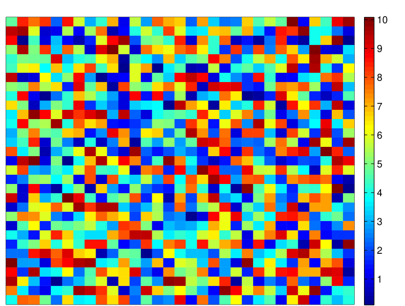
(a) Lamé coefficient $\mu$

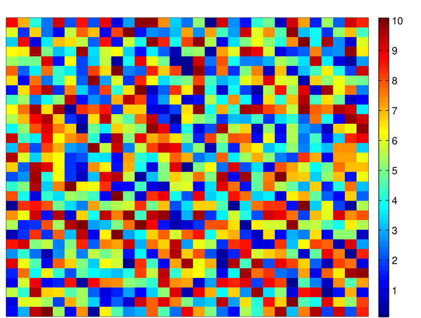
(b) Lamé coefficient $\lambda$

Figure 1. Lamé coefficients with multiscale features.

For the numerical approximations we discretize the domain with a uniform triangulation. The reference solution $u_{h}$ in (3.1) is computed using a mesh of size $h=\sqrt{2}\cdot 2^{-6}$, which is small enough to resolve the multiscale coefficients in Figure 1. The generalized finite element (GFEM) solution in (4.4) is computed on several meshes of decreasing size, $H=\sqrt{2}\cdot 2^{-1},...,\sqrt{2}\cdot 2^{-5}$ with $k=1,1,2,2,3$, which corresponds to $k=\lceil 0.8\log H^{-1}\rceil$. These solutions are compared to the reference solution. For comparison we also compute the classical piecewise linear finite element (P1-FEM) solution on the meshes of size $H=\sqrt{2}\cdot 2^{-1},...,\sqrt{2}\cdot 2^{-5}$. The error is computed using the $H^{1}$ semi-norm $\|\nabla\cdot\|$ and plotted in Figure 2.

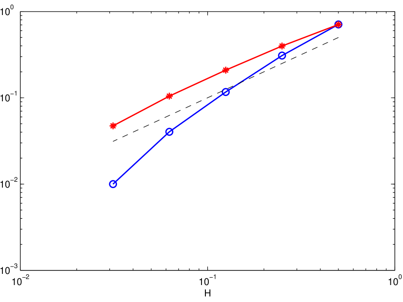
(a) Constant coefficients $\mu=\lambda=1$.

(b) Multiscale coefficients, see Figure 1.

Figure 2. Relative errors using GFEM (blue $\circ$) and P1-FEM (red $\ast$) for the linear elasticity problem plotted against the mesh size $H$. The dashed line is $H$.

In Figure 2 we see that both methods, as expected, show linear convergence for the problem with constant coefficients. For the problem with multiscale coefficients we clearly see the advantages with the generalized finite element method, which shows linear convergence also in this case, while the classical finite element shows far from optimal convergence.

For the second experiment we aim to test the locking effect. We consider a problem from [6]. The domain is set to the unit square $\Omega=[0,1]\times[0,1]$ and $g_{D}=0$ on the boundary $\Gamma_{D}=\partial\Omega$. Furthermore, with $\mu=1$ and the right hand side $f=[f_{1}\ f_{2}]^{\intercal}$ chosen as

$$f_{1} =\pi^{2}\Big{(}4\sin(2\pi y)(-1+2\cos(2\pi x))-\cos\pi(x+y)+\frac{2}{1+\lambda}\sin(\pi x)\sin(\pi y)\Big{)},$$

$$f_{2} =\pi^{2}\Big{(}4\sin(2\pi y)(1-2\cos(2\pi x))-\cos\pi(x+y)+\frac{2}{1+\lambda}\sin(\pi x)\sin(\pi y)\Big{)},$$

the exact solution $u=[u_{1}\ u_{2}]^{\intercal}$ is given by

$$u_{1} =\sin(2\pi y)(-1+2\cos(2\pi x))+\frac{1}{1+\lambda}\sin(\pi x)\sin(\pi y),$$

$$u_{2} =\sin(2\pi y)(1-2\cos(2\pi x))+\frac{1}{1+\lambda}\sin(\pi x)\sin(\pi y).$$

In this experiment we let $\lambda=10^{3}$. The discretization of the domain remain the same as in our first example, but the size of the reference mesh is set to $h=\sqrt{2}\cdot 2^{-7}$ which is sufficiently small for $u_{h}$ to be a relatively good approximation, since $h<1/\sqrt{\lambda}$. Indeed, using the knowledge of the exact solution we have $\|\nabla(\mathcal{I}_{h}(u)-u_{h})\|_{L_{2}(\Omega)}/\|\nabla\mathcal{I}_{h}(u)\|_{L_{2}(\Omega)}\approx 0.15$, where $\mathcal{I}_{h}$ is the Lagrangian nodal interpolation onto $V_{h}$.

The GFEM and the classical P1-FEM solutions are computed for the values $H=\sqrt{2}\cdot 2^{-1},...,\sqrt{2}\cdot 2^{-6}$. The localization parameter is chosen to be $k=1,1,2,2,3,4$ which corresponds to $k=\lceil 0.8\log H^{-1}\rceil$. The numerical approximations $u_{\mathrm{ms},k}$ and $u_{H}$ are compared to the reference solution $u_{h}$ and the error is computed using the $H^{1}$-seminorm. The relative errors are plotted in Figure 3. Clearly, the classical finite element method suffers from locking effects for the coarser mesh sizes. However, the generalized finite element solution shows linear convergence, that is, no locking effect is noted.

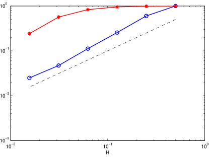
Figure 3. Relative errors for the locking problem using GFEM (blue $\circ$) and P1-FEM (red $\ast$) plotted against the mesh size $H$. The dashed line is $H$.

References

- [1] A. Abdulle. Analysis of a heterogeneous multiscale FEM for problems in elasticity. Math. Models Methods Appl. Sci., 16(4):615–635, 2006.
- [2] A. Abdulle and P. Henning. Localized orthogonal decomposition method for the wave equation with a continuum of scales. ArXiv e-print 1406.6325, to appear in Math. Comp., 2016+.
- [3] D. N. Arnold, R. S. Falk, and R. Winther. Mixed finite element methods for linear elasticity with weakly imposed symmetry. Math. Comp., 76(260):1699–1723, 2007.
- [4] I. Babuška and J. E. Osborn. Generalized finite element methods: their performance and their relation to mixed methods. SIAM J. Numer. Anal., 20(3):510–536, 1983.
- [5] I. Babuska and M. Suri. Locking effects in the finite-element approximation of elasticity problems. Numerische Mathematik, 62(4):439–463, 1992.
- [6] S. C. Brenner. A nonconforming mixed multigrid method for the pure displacement problem in planar linear elasticity. SIAM J. Numer. Anal., 30(1):116–135, 1993.
- [7] S. C. Brenner and R. L. Scott. The mathematical theory of finite element methods, volume 15 of Texts in Applied Mathematics. Springer, New York, third edition, 2008.
- [8] S. C. Brenner and L.-Y. Sung. Linear finite element methods for planar linear elasticity. Math. Comp., 59(200):321–338, 1992.
- [9] F. El Halabi, D. González, A. Chico, and M. Doblaré. multiscale in linear elasticity based on parametrized microscale models using proper generalized decomposition. Comput. Methods Appl. Mech. Engrg., 257:183–202, 2013.
- [10] C. Engwer, P. Henning, A. Målqvist, and D. Peterseim. Efficient implementation of the localized orthogonal decomposition method. ArXiv e-print 1602.01658, 2016.
- [11] D. Gallistl and D. Peterseim. Stable multiscale Petrov-Galerkin finite element method for high frequency acoustic scattering. Comput. Methods Appl. Mech. Engrg., 295:1–17, 2015.
- [12] J. M. Gere and B. J. Goodno. Mechanics of Material. Cengage Learning, 2008.
- [13] P. Henning and A. Målqvist. Localized orthogonal decomposition techniques for boundary value problems. SIAM J. Sci. Comput., 36(4):A1609–A1634, 2014.
- [14] P. Henning, A. Målqvist, and D. Peterseim. A localized orthogonal decomposition method for semi-linear elliptic problems. ESAIM Math. Model. Numer. Anal., 48(5):1331–1349, 2014.
- [15] P. Henning, A. Målqvist, and D. Peterseim. Two-Level Discretization Techniques for Ground State Computations of Bose-Einstein Condensates. SIAM J. Numer. Anal., 52(4):1525–1550, 2014.
- [16] P. Henning and D. Peterseim. Oversampling for the Multiscale Finite Element Method. SIAM Multiscale Model. Simul., 11(4):1149–1175, 2013.
- [17] T. J. R. Hughes, G. R. Feijóo, L. Mazzei, and J.-B. Quincy. The variational multiscale method—a paradigm for computational mechanics. Comput. Methods Appl. Mech. Engrg., 166(1-2):3–24, 1998.
- [18] T. J. R. Hughes and G. Sangalli. Variational multiscale analysis: the fine-scale Green’s function, projection, optimization, localization, and stabilized methods. SIAM J. Numer. Anal., 45(2):539–557, 2007.
- [19] M. G. Larson and A. Målqvist. Adaptive variational multiscale methods based on a posteriori error estimation: energy norm estimates for elliptic problems. Comput. Methods Appl. Mech. Engrg., 196(21-24):2313–2324, 2007.
- [20] A. Målqvist. Multiscale methods for elliptic problems. Multiscale Model. Simul., 9(3):1064–1086, 2011.
- [21] A. Målqvist and A. Persson. Multiscale techniques for parabolic equations. Submitted, 2015.
- [22] A. Målqvist and D. Peterseim. Localization of elliptic multiscale problems. Math. Comp., 83(290):2583–2603, 2014.
- [23] A. Målqvist and D. Peterseim. Computation of eigenvalues by numerical upscaling. Numer. Math., 130(2):337–361, 2015.
- [24] A. Masud and K. Xia. A variational multiscale method for inelasticity: application to superelasticity in shape memory alloys. Comput. Methods Appl. Mech. Engrg., 195(33-36):4512–4531, 2006.
- [25] A. L. Mazzucato and V. Nistor. Well-posedness and regularity for the elasticity equation with mixed boundary conditions on polyhedral domains and domains with cracks. Arch. Ration. Mech. Anal., 195(1):25–73, 2010.
- [26] P. H. Mott and C. M. Roland. Limits to poisson’s ratio in isotropic materials. Physical Review B, 80(13), OCT 2009.
- [27] D. Peterseim. Eliminating the pollution effect in helmholtz problems by local subscale correction. Submitted, 2015.
- [28] D. Peterseim. Variational Multiscale Stabilization and the Exponential Decay of Fine-scale Correctors. To appear, 2015/16.
- [29] B. Xia and V. H. Hoang. High-dimensional finite element method for multiscale linear elasticity. IMA J. Numer. Anal., 35(3):1277–1314, 2015.