Image Retrieval with a Bayesian Model of Relevance Feedback

Abstract

A content-based image retrieval system based on multinomial relevance feedback is proposed. The system relies on an interactive search paradigm where at each round a user is presented with $k$ images and selects the one closest to their ideal target. Two approaches, one based on the Dirichlet distribution and one based the Beta distribution, are used to model the problem motivating an algorithm that trades exploration and exploitation in presenting the images in each round. Experimental results show that the new approache compares favourably with previous work.

1 Introduction

We consider content-based image (CBIR) retrieval in the case when the user is unable to specify the required content through tags or other image properties. In this type of scenario, the system must extract information from the user through limited feedback. We consider a protocol that operates through a sequence of rounds in each of which a set of images is displayed and the user must indicate which image is closest to their ideal target image(s). Note that we do not always assume that the target image(s) is/are in the database. Instead, we test two hypotheses as to what constitutes the user’s target. In our first hypothesis, we assume there is a hypothetical target single image in the user’s mind. Our second hypothesis assumes that there is a set of images, any of which will satisfy the user. Clearly, in both scenarios, the user search concludes in a single image. However, each of the two hypotheses differs in terms of how the user perceives the search procedure. In the former case, the system’s assumption is that the user has a precise image in their mind from the beginning of the search session and so the system will try to converge on a particular single image from the first iteration of the search. Unfortunately, this approach might fail if the user is not very familiar with the database they are searching or does not concentrate on finding a specific image and so uses the initial couple of iterations in a more exploratory fashion in order to “familiarise” himself with the image database and better formulate his search target. In the latter hypothesis, the user has a vague notion of the kind of image that is required and wants to explore the current database while at the same time trying to decide what the final target image should be. While the problem of image retrieval with relevance feedback has been studied before (e.g. [3, 6, 8]), we present a novel Bayesian approach that uses latent random variables to model the system’s imperfect knowledge about the user’s expected response to the images. The proposed approach compares favourably with previous work.

For our first hypothesis, suppose we are given a database $\mathscr{D}$ of images. For each image $x_{i}\in\mathscr{D}$, we use a latent variable $\theta_{i}$ taking values in $[0,1]$ to represent the chance that $x_{i}$ is the image the user is searching for. Supposing that the user has a single ideal target, the variables have to sum to one: $\sum_{x_{i}\in\mathscr{D}}\theta_{i}=1.$ Since the system has incomplete knowledge about the user’s target image, it uses a Dirichlet distribution over the variables $(\theta_{i})$ to represent the state of its knowledge. Thus we call our algorithm Dirichlet Sampling (DS) [10]. At each iteration, the system samples $k$ images to present to the user, from which the user selects the one closest to the target. An important aspect of the DS algorithm is the way in which its knowledge of the target is updated given user feedback. We considered two algorithms to do so: variational Bayes and Gibbs sampling.

We compare the performance of the DS algorithm with that of Beta Experts (BE), where uniform updates are used to improve the system’s knowledge of the target. The assumption of the BE algorithm is that instead of there being a single target image, there is a set of images, any of which will satisfy the user. Thus, we give uniform updates to all the images that are considered to be the user’s preferred images. For each image $x_{i}\in\mathscr{D}$, there is a random variable $b_{i}$ which models whether image $x_{i}$ is a preferred image. The probability that $x_{i}$ is a preferred image is modelled using a number $p_{i}\in[0,1]$. Since $p_{i}$ is unknown, we model it as an unobserved random variable with a beta prior $\varpropto p_{i}^{a-1}(1-p_{i})^{b-1}$. We show in experiments that the simple uniform update performs best. The reason is because both variational Bayes and Gibbs sampling tend to focus on a small set of images (which may or may not contain the target) aggressively, while the uniform update is less aggressive.

An important aspect of both approaches is the incorporation of an explicit exploration-exploitation strategy in the image sampling process, which greatly improves the performance of the algorithms compared to their main competitors that do not employ exploration-exploitation strategies. Our approach is similar to Thompson sampling [5]. In the case of the DS algorithm, a sample is drawn from the Dirichlet distribution which represents the knowledge state of the system, adjusted using a temperature to trade-off exploration and exploitation, and the image with the largest probability (in the sample) of being the target is selected; this is repeated $k$ times to obtain the $k$ images presented. We employ a similar approach in the case of the BE algorithm, where we sample $k$ images from the Beta distribution.

In summary, our system supports the user in finding an image that best matches their query in the manner described below. In each iteration, $k$ images from the database $\mathscr{D}$ are presented to the user and the user selects the most relevant image from this set, according to the following protocol:
For each iteration $i=1,2,\ldots$ of the search:

• Search engine calculates a set of images ${\mathbf{x}}_{i,1},\ldots,{\mathbf{x}}_{i,k}\in\mathscr{D}$ to present to the user.

• If one of the images matches the user’s query, then the search terminates.

• Otherwise, the user chooses one of the images ${\mathbf{x}}_{i}^{\ast}$ as most relevant according to a distribution $D\{{\mathbf{x}}_{i}^{\ast}={\mathbf{x}}_{i,j}\mid{\mathbf{x}}_{i,1},\ldots,{\mathbf{x}}_{i,k};\mathbf{t}\}$, where $\mathbf{t}$ denotes the target image. Note that $\mathbf{t}$ can be either a single image or a representation of the target set of images.

2 The Dirichlet Search Algorithm

In this section, we introduce the main aspects of the DS algorithm. Let $\mathscr{D}$ be a dataset of $n$ images $({\mathbf{x}}_{i})_{i=1,\ldots,n}$. Let $M=\{m_{1},\ldots,m_{n}\}$ the base measure defined on $\mathscr{D}$ and $\alpha$ the number of pseudocounts. Initially, we set $(m_{i})_{i=1,\ldots,n}=\frac{1}{n}$ and $\alpha=1$. Let ${\mathbf{x}}_{j}^{\ast}\in\{{\mathbf{x}}_{j,1},\ldots,{\mathbf{x}}_{j,k}\}$ be the image chosen by the user at iteration $j$ from among the $k$ presented images $\{{\mathbf{x}}_{j,1},\ldots,{\mathbf{x}}_{j,k}\}$. We suppress the index $j$ to simplify the exposition. In our model, the user only sees $k$ images at each iteration and so we can only observe user’s preference with respect to these $k$ images. However, we want to be able to model the user’s preferences with respect to the entire dataset of images. Thus, we view the set of images $\{{\mathbf{x}}_{1},\ldots,{\mathbf{x}}_{k}\}$ as partitioning the complete space of images into sets $\mathscr{X}_{1},\ldots,\mathscr{X}_{k}$ with

$$\mathscr{X}_{j}=\{\mathbf{x}:d({\mathbf{x}}_{j},{\mathbf{x}})<d({\mathbf{x}}_{j^{\prime}},{\mathbf{x}}),j^{\prime}\neq j\}.$$ (1)

In order to be able to update the base measures of all images in a given partition at each iteration and be able to approximate the true Dirichlet posterior, we derive the base measure updates using Variational Bayes (VB) [2, 4, 11, 12]. In Section 6.2, we also compare the performance of the DS algorithm with VB updates and updates obtained through Gibbs sampling.

2.1 VB Parameter Updates

Below we illustrate the factorized variational approximation for the Dirichlet Search algorithm. Dirichlet distributions $Dir({\bf\alpha})$ are probability distributions over multinomial parameter vectors. The distribution is parametrised by a vector ${\bf\alpha}=\{\alpha_{1},\ldots,\alpha_{n}\}$, where $\alpha=(\alpha_{1},\ldots,\alpha_{n})=\alpha_{0}(m_{1},\ldots,m_{n})$, where $(m_{1},\ldots,m_{n})$ has 1-norm 1 and $\alpha_{0}>1$. The Dirichlet distribution is conjugate to the Multinomial distribution, which gives us the following generative model:

$${\bf\theta|\alpha}\backsim Dir({\bf\alpha})$$

$$\beta_{i}|{\bf\theta}\backsim Mult({\bf\theta})$$

As mentioned earlier, at each iteration, the user is presented with $k$ images and selects one of them as being “most similar” to the their ideal target image. The selected image is a “proxy” for similar images, which we also consider to be selected by the user. Thus, we want to apply different updates depending on whether a given image was in a partition $\pi$ selected by the user. Given a set $\{x_{1},\ldots,x_{k}\}$ of observed images, the user selects image $x_{j}^{\star}$, which is the proxy for the partition containing that particular image. We denote the partition containing image $x_{j}^{\star}$ as $\pi_{x_{j}^{\star}}$. Our generative model looks as follows:

$$P({\bf\theta|\alpha})\varpropto\prod_{i}^{N}\theta_{i}^{\alpha_{i}-1}$$ (2)

$$P({\bf\beta|\theta})=\prod_{i}^{N}\theta_{i}^{\beta_{i}}$$ (3)

$$P(x_{j}^{\star}\mid{\bf\beta},\pi)=\delta\begin{cases}1&\text{if}\quad\beta_{i}\in\pi_{x_{j}^{\star}}\\ 0&\text{otherwise}\end{cases}$$ (4)

Given our variables ${\bf\theta}$ and $\beta$, and the selected image $x_{j}^{\star}$, we wish to obtain $p({\bf\theta,\beta})|x_{j}^{\star}$. For most models, this is intractable and so we consider distribution $q({\bf\theta,\beta})$, which can be factorised as:

$$q({\bf\theta,\beta})=q_{\theta}({\bf\theta})q_{\beta}({\bf\beta})$$ (5)

which gives us the following definition of $F(q)$:

$$F(q)=\int q_{\theta}({\bf\theta})q_{\beta}({\bf\beta})\log\frac{p(x_{j}^{\star},{\bf\theta,\beta})}{q_{\theta}({\bf\theta})q_{\beta}({\bf\beta})}d{\bf\theta}d{\bf\beta}$$ (6)

The computation of $q({\bf\theta})$ proceeds by its maximisation of $F(q)$:

$$\log q_{\theta}({\bf\theta})=\int q_{\beta}({\bf\beta})\log p(x_{j}^{\star},{\bf\theta,\beta})d{\bf\beta}$$ (7)

We can rewrite Eq. 7 in terms of an expectation:

$$\log q_{\theta}({\bf\theta})=\mathbb{E}_{q(\beta)}[\log p(x_{j}^{\star},{\bf\theta,\beta})d{\bf\beta}]$$ (8)

$$q_{\theta}({\bf\theta})\varpropto\exp(\mathbb{E}_{q(\beta)}[\log p(x_{j}^{\star},{\bf\theta,\beta})d{\bf\beta}])$$ (9)

Applying the same procedure with respect to $q(\beta)$ will give us:

$$q_{\beta}({\bf\beta})\varpropto\exp(\mathbb{E}_{q(\theta)}[\log p(x_{j}^{\star},{\bf\theta,\beta})d{\bf\beta}])$$ (10)

We apply the result (8) to find the expression for the optimal factor $q_{\theta}({\bf\theta})$. We only need to retain the those terms that have functional dependency on $\theta$ as all the remaining terms are absorbed into the normalising constant. Thus, we have:

$$\log q_{\theta}(\theta_{i})=\mathbb{E}_{q(\beta_{i})}[\log p(\theta_{i})+\log p(\beta_{i})]+C$$ (11)

$$=\mathbb{E}_{q(\beta_{i})}[\log(\theta_{i}^{\alpha_{i}-1})+\log(\theta_{i}^{\beta_{i}})]+C$$ (12)

$$=\mathbb{E}_{q(\beta_{i})}[(\alpha_{i}-1+\beta_{i})\log\theta_{i}]+C$$ (13)

$$=\alpha_{i}-1+\mathbb{E}[\beta_{i}\log\theta_{i}]+C$$ (14)

We can identify that

$$q_{\theta}(\theta_{i})=Dir(\theta|\alpha_{i})$$ (15)

where

$$\alpha_{i}^{\star}=\alpha_{i}+\mathbb{E}[\beta_{i}]$$ (16)

Similarly, we can obtain the expression for the optimal $q_{\beta}({\bf\beta})$:

$$\log q_{\beta}(\beta_{i})=\mathbb{E}_{q(\theta_{i})}[\log(\beta_{i})+\log(x_{j}^{\star})]+C$$ (17)

$$=\mathbb{E}_{q(\theta_{i})}[\log(\theta_{i}^{\beta_{i}})+\log\delta]+C$$ (18)

$$=\mathbb{E}_{q(\theta_{i})}[\beta_{i}\log\theta_{i}+\log\delta(x_{i})]+C$$ (19)

$$=\beta_{i}\mathbb{E}[\log\theta_{i}]+\log\delta(x_{i})+C$$ (20)

We can see that

$$q_{\beta}(\beta_{i})=Mult(\beta_{i}|\gamma_{i})$$ (21)

where

$$\gamma_{i}\varpropto\begin{cases}0&\text{if}\quad x_{i}\notin\pi_{x_{j}^{\star}}\\ e^{\mathbb{E}[\log\theta_{i}]}&\text{otherwise}\end{cases}$$ (22)

Note that for Dirichlet distributions [1],

$$e^{\mathbb{E}[\log\theta_{i}]}\approx\max(0,\alpha_{i}-.5)$$ (23)

so that the update for $\alpha_{i}$ is approximately:

$$\alpha_{i}^{*}\approx\alpha_{i}+\begin{cases}\frac{\max(0,\alpha_{i}-.5)}{\sum_{i:x_{i}\in\mathscr{X}_{j}}\max(0,\alpha_{i}-.5)}&\text{if $x_{i}\in\mathscr{X}_{j}$}\\ 0&\text{otherwise}\end{cases}$$ (24)

In other words, the parameters of images in the chosen partition are incremented, with the total increment equal to 1. Further, images $x_{i}$ whose parameter $\alpha_{i}$ is already large tend to get a larger share of the increment, while those with small $\alpha_{i}$ will not get much increment at all. This effect, where the “rich-get-richer” can easily force the VB algorithm into a situation where the parameters for a small set of images dominates, even though they are not the true image. The resulting image search algorithm will then never converge to the true image since it will always show one of these dominating images.

To address this problem of premature (and wrong) convergence, we propose a simple approach whereby all images in the chosen partition get incremented by an equal amount. The approach is based on the Beta distribution and we call it the Beta Experts algorithm.

3 The Beta Experts Algorithm

Let $\mathscr{D}$ index the set of images. Instead of assuming that the user’s (latent) preference is a single true image, we will assume that there is a set of images, any of which will satisfy the user, i.e. if the user saw one of these images during one of the rounds, the procedure would terminate with success. In other words, for each $x_{i}\in\mathscr{D}$, there is a binary indicator $b_{i}^{\star}\in\{0,1\}$, where $b_{i}^{\star}=1$ if image $x_{i}$ is one of the user’s preferred images, and $b_{i}^{\star}=0$ otherwise.

For each image $x_{i}\in\mathscr{D}$, let $b_{i}$ be a random variable which will model whether image $x_{i}$ is a preferred image or not. The value of $b_{i}$ is unknown to the system thus modelled as an unobserved random variable.

The probability that $x_{i}$ is a preferred image, i.e. that $b_{i}=1$, is modelled using a number $p_{i}\in[0,1]$. Since $p_{i}$ is unknown, we will also model it as an unobserved random variable, with a beta prior $\varpropto p_{i}^{a-1}(1-p_{i})^{b-1}$.

The system shows the user $k$ images in each of rounds $r=1,\ldots,R$. In round $r$ the $k$ images are indexed by $C_{r}=\{x_{i_{r1}},\ldots,x_{i_{rk}}\}$. The user either sees an image she is looking for (a preferred image), in which case the system terminates with success, or the user will choose an image $k_{r}$ from among the $k$ shown that is “closest” to the preferred images in her mind.

We model the user’s choices as follows. At round $r$ let $I_{r1},\ldots,I_{rk}$ be a partition of the set of images $\mathscr{D}$, such that $I_{rj}$ contains all images such that $x_{i_{rj}}$ is the closest image to it among $x_{i_{r1}},\ldots,x_{i_{rk}}$ . We model the joint probability of choices and preference probabilities as an exponential family harmonium:

$$P(k_{1},\ldots,k_{R},\{p_{i}\}_{i\in\mathscr{D}})\propto$$

$$\prod_{i\in\mathscr{D}}p_{i}^{a-1}(1-p_{i})^{b-1}\prod_{r=1}^{R}\prod_{i\in I_{rk_{r}}}p_{i}\prod_{i\notin I_{rk_{r}}}(1-p_{i})$$ (25)

Given the choices of the users up to round $R$, the posterior distribution over $\{p_{i}\}$ is:

$$P(\{p_{i}\}_{i\in I}\mid k_{1},\ldots,k_{R})$$

$$\propto\prod_{i\in\mathscr{D}}p_{i}^{a-1}(1-p_{i})^{b-1}\prod_{r=1}^{R}\prod_{i\in I_{rk_{r}}}p_{i}􏰒\prod_{i\notin I_{rk_{r}}}(1-p_{i})$$ (26)

$$\propto\prod_{i\in\mathscr{D}}p_{i}^{a+n_{i}-1}(1-p_{i})^{b+R-n_{i}-1}$$ (27)

where $n_{i}=\varhash\{r:i\in I_{rk_{r}}\}$ is the number of user choices such that $i$ is in the closest partition. Incidentally, note that the conditional probability that the user will pick $k_{r}$ out of the $k$ images at round $r$ is:

$$P(k_{r}\mid\{p_{i}\})\propto\prod_{i\in I_{rk_{r}}}p_{i}\prod_{i\notin I_{rk_{r}}}(1-p_{i})$$ (28)

$$\propto\ e^{\sum_{i\in I_{rk_{r}}}\log p_{i}/(1-p_{i})}$$ (29)

is a softmax of the sum of log odds-ratios over images in partition $I_{rk_{r}}$.

In Section 6.2, we compare the performance of the DS algorithm with the VB updates and the BE algorithm.

4 Balancing Exploration versus Exploitation

The final ingredient of the DS and the BE algorithms is how the images presented to the user should be chosen. This involves a trade-off between presenting images that appear promising based on best current estimates of the mean given by the posterior measure (exploitation), and trying areas where our current estimate could be too pessimistic (exploration). The strategy we adopt to solve this problem is to draw $k$ samples from the posterior distribution, where each sample corresponds to distribution over all the images, and select the images $\mathbf{x}_{j}$, where $j=1,\ldots,k$, that have the highest probability in each of these samples. In case of the DS algorithm, we obtain this by sampling from the Dirichlet distribution. A fast method to sample a random vector from a $n$-dimensional Dirichlet distribution with parameters $m=\{\alpha m_{1},\ldots,\alpha m_{n}\}$ is to draw $n$ independent random samples from the gamma distribution: $f_{i}\sim Gamma(\alpha m_{i},1)=\frac{f_{i}^{\alpha m_{i}-1}e^{-f_{i}}}{\Gamma(\alpha m_{i})}$, and normalise the resulting vector. Since we are interested only in the maximum, we can omit the normalisation step (Algorithm 1).

Algorithm 1 Image selection for the DS algorithm

  for $\mathtt{j}=1,\ldots,k$ do

     for $i=1,\ldots,n$ do

        $f_{i}\leftarrow\mathtt{randg}(\alpha m_{i})$

     end for

     $[\mathtt{value}_{j},\mathtt{index}_{j}]\leftarrow\max(f)$; $\mathtt{images}_{\mathtt{j}}\leftarrow\mathtt{index}_{j}$

  end for

  Return: array $\mathtt{images}$ with indices of selected images

In case of the BE algorithm, we draw $n$ independent samples from the beta distribution and select the maximum (Algorithm 2).

Algorithm 2 Image selection for the BE algorithm

  for $\mathtt{j}=1,\ldots,k$ do

     for $i=1,\ldots,n$ do

        $\mathtt{r}_{a_{i}}\leftarrow\mathtt{randg}(a_{i})$

        $\mathtt{r}_{b_{i}}\leftarrow\mathtt{randg}(b_{i})$

        $f_{i}=\frac{\mathtt{r}_{a_{i}}}{\mathtt{r}_{a_{i}}+\mathtt{r}_{b_{i}}}$

     end for

     $[\mathtt{value}_{j},\mathtt{index}_{j}]\leftarrow\max(f)$; $\mathtt{images}_{\mathtt{j}}\leftarrow\mathtt{index}_{j}$

  end for

  Return: array $\mathtt{images}$ with indices of selected images

5 The user model

We assume that the choice of one of the presented images is a random process, where more relevant images are more likely to be chosen. This models some source of noise in the user’s selection process. In our simulation experiments reported in the next section, we will rely on the user model proposed by [3]. The prediction of this particular user model has been shown to be compatible with the actual user behaviour [9]. In Section 6.4, we also compare the performance of the algorithms in real-life and in simulations. Following [3], we assume a similarity measure $S({\mathbf{x}}_{1},{\mathbf{x}}_{2})$ between images ${\mathbf{x}}_{1},{\mathbf{x}}_{2}$, which also measures the relevance of an image ${\mathbf{x}}$ compared to an ideal target image $\mathbf{t}$ by $S(\mathbf{x},\mathbf{t})$. We assume that in the case of the DS algorithm, $\mathbf{t}$ is the ideal target image, while in the case of the BE algorithm, $\mathbf{t}$ is the centre of the partition containing images preferred by the user. Let $0\leq\lambda\leq 1$ be the uniform noise in the user’s choice. The probability of choosing image ${\mathbf{x}}_{i,j}$ is given by:

$$D\{{\mathbf{x}}_{i}^{\ast}={\mathbf{x}}_{i,j}\mid{\mathbf{x}}_{i,1},\ldots,{\mathbf{x}}_{i,k};\mathbf{t}\}=(1-\lambda)\frac{S({\mathbf{x}}_{i,j},\mathbf{t})}{\sum_{j=1}^{k}S({\mathbf{x}}_{i,j},\mathbf{t})}+\frac{\lambda}{k}.$$ (30)

Assuming a distance function $d(\cdot,\cdot)$, a possible choice for the similarity measure $S(\cdot,\cdot)$ is

$$S({\mathbf{x}},\mathbf{t})=d({\mathbf{x}},\mathbf{t})^{-a}$$ (31)

with parameter $a>0$. This particular measure decreases polynomially with increasing distance. The parameter $a>0$ indicates the user “sharpness”. Large $a$ implies that the user favours images closer to the target image. With the polynomial similarity measure, the user’s response depends on the relative size of the image distances to the ideal target image.

We use the Euclidean norm

$$d({\mathbf{x}},\mathbf{t})=\parallel{\mathbf{x}}-\mathbf{t}\parallel$$ (32)

as the distance measure between image ${\mathbf{x}}$ and the target image $\mathbf{t}$. In all the experiments reported below, the values of $a$ and $\lambda$ in the user model were kept constant at 2 and 0.1, respectively (these were the optimal values based on [9]).

6 Experiments

We tested the performance of the DS and the BE algorithms in simulations and in real-life experiments. The aim of the simulation experiments was to assess which one of the proposed models achieves better results, while the aim of the real-life experiments was to confirm the compatibility of the user model with the real user behaviour. In all the experiments, we used a subset of the Tiny Images Dataset [13] with 758 categories and 37900 images. We used the Basic Image Features (BIFs) technique [7] to extract the image features. During the experiments, we measured two things: (1) the average number of iterations required by each method to find the target image; and (2) the average distance of the $k$ images presented at each iteration from the target image(s).

6.1 Simulation experiments

All the reported results from the simulation experiments are averaged over 1000 searches for randomly selected target images from the dataset. In all the experiments reported in this section, we employed the user model described in Section 5.

Table 1: Comparison of the performance of the DS algorithm with VB updates (VB) and the Beta Experts (BE) algorithm

	k =	2	k =	5	k =	10
Target Size	BE	VB	BE	VB	BE	VB
1	69	450	26	198	17	86
5	47	431	19	89	14	38
10	41	393	17	60	11	22

In the first set of experiments, we compared the performance of the DS algorithm with VB updates with the BE algorithm. Table 1 shows the average number of iterations to find the target image with both algorithms as the value of $k$ increases. We also measured the number of iterations required by each algorithm to get to the target that consists only of the ideal target image (target size = 1) or the target image plus a number of images close to it. As the experimental results show, the BE algorithm significantly outperform the DS algorithm with the VB updates. A possible explanation might be the value of the updates, which are smaller in case of VB updates. In case of the BE algorithm, the weights of more promising images are increased by a uniform value of 1, which allows the algorithm to sample more relevant images early on in the search. The other possibility is that VB zooms in on a particular image too quickly and through future updates cannot easily recover from the initial “wrong” choices by the user.

6.2 Gibbs Sampling and the Dirichlet Search Algorithm

As the experimental results reported in the previous section show, the DS algorithm with VB updates performs much worse than the BE algorithm. VB provides only an approximate of the “true” posterior. In the next set of experiments, we apply Gibbs sampling to obtain a better approximation of the posterior. Gibbs sampling is applicable when the joint distribution is not known explicitly or is difficult to sample from directly, but the conditional distribution of each variable is known and is easy to sample from. Gibbs sampling generates an instance from the distribution of each variable in turn, conditional on the current values of the other variables. The sequence of samples constitutes a Markov chain, and the stationary distribution of that Markov chain is the sought – after joint distribution that we try to approximate. Due to the Markovian properties, the approximation of the joint distribution derived through Gibbs sampling is usually more accurate than that provided by VB.

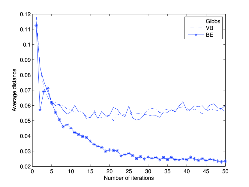
Figure 1: Convergence of the DS algorithm with a Gibbs sampler and VB updates, and the Beta Experts (BE) algorithm.

The Gibbs sampler that we used in our experiments is summarised in Algorithm 3 below.

Algorithm 3 Gibbs sampler for the DS algorithm

  input: base measures $m_{1,\ldots,n}=\frac{1}{n}$;

  matrix $C\quad z\times k$ with $k$ images presented at iterations $1,\ldots,z$

  for $j=1,\ldots,k$ do

     for $i=1,\ldots,100$ do

        for $l=1,\ldots,z$ do

           $s=\sum_{h\in O_{l}}^{n}m_{i}^{i-1}$, where $O_{l}$ is partition containing image $C_{y,l}$

           $r_{h}=\frac{m_{h}}{s}\quad h\in O_{l}$

           $v_{l}\sim Mult((r_{h})_{h\in O_{l}})$

        end for

        $b_{h}=m_{h}^{i-1}+\sum_{l=1}^{z}1(v_{l}=h)$

        $m_{h}^{s}\sim Dir(b_{h})$

     end for

     $g_{j}=Gamma(m^{s})$

     [value, index] = max($g_{j}$)

  end for

  return: array $images$ with indices of selected images

Table 2: Comparison of the AL algorithm, the Beta Experts (BE) algorithm and PicHunter (PH)

	k	=	2	k	=	5	k	=	10
Target Size	AL	BE	PH	AL	BE	PH	AL	BE	PH
1	227	69	482	117	26	422	92	17	374
5	167	47	461	81	19	390	59	14	328
10	139	41	454	64	17	370	48	11	308

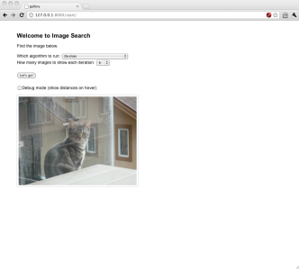
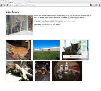
Figure 2: User interface of the image search prototype system.

Figure 1 shows the average distance from the target of 10 images presented to the user over the first 50 iterations of the algorithm. The results are averaged over 1000 runs of the search algorithm with a random target image selected in each run. As the results show, incorporating Gibbs sampling into the search procedure does not improve the performance of the DS algorithm, indicating that the poor performance is not as a result of the approximate inference but of a poor model, i.e. the correct Bayesian model is inferior to the Beta Experts model, indicating that the assumption that users have a set of images rather than a single target image is a better reflection of the users’ behaviour.

6.3 Related image retrieval algorithms and experimental results

In the last set of simulation experiments, we compare the BE algorithm against two alternatives: the search algorithm proposed in [3] (we call it the AL algorithm) and PicHunter [6]. We used the same experimental setting as in the experiments described above. We selected these two algorithms as our benchmark due to the fact that, similarly to our approach, they combine a relevance feedback model with an exploration–exploitation trade-off.

The AL algorithm proposes a weighting scheme that demotes all apparently less relevant images by a constant discount factor $0\leq\beta<1$. Initially, all the weights $w_{i}=1$. After each iteration, all the images close to the one selected by the user stay unchanged, while all the remaining images are demoted by $\beta$. We set the value of $\beta=0.5$ as this was the value that gave the best experimental results.

The PicHunter image retrieval system uses Bayes’ rule to predict the user’s target image. The system maintains a set of probabilities for every image. Initially, all the probabilities $p_{i}=\frac{1}{n}$. During each iteration, the search engine displays a set of images and the user selects an image. The probabilities are updated as in $p_{i}=p_{i}*G(d(x_{i},s_{m}))$, where $d(x_{i},s_{m})=\parallel x_{i}-s_{m}\parallel$ is the distance between image $x_{i}$ and image $s_{m}$ selected by the user in iteration $m$, and $G$ is defined as

$$G=\frac{\exp(-d(x_{i},s_{m})/\sigma)}{\sum_{j=1}^{n}\exp(-d(x_{j},s_{m})/\sigma)}$$ (33)

In all the experiments reported here $\sigma=0.3$. After each iteration, $k$ images with the highest $p$ are displayed.

We calculated the average number of iterations to terminate the search as the value of $k$ increases (Table 2). We tested the scaling properties of the algorithm by increasing the size of the image target set, while keeping the size of the image database constant, i.e. the search terminates when one of the 5 or 10 images closest to the target is presented.

The BE algorithm significantly outperforms the AL algorithm and PicHunter. The disappointing performance of the AL algorithm might be attributed to downgrading the weights by a constant value $\beta$. If during the initial iterations the user selects an image far away from the target, the weights of the images close to the target will be demoted early on in the search thus making them less likely to be sampled in the future. PicHunter does not really have an exploration stage – rather than sampling images, at each iteration only the $k$ images with the highest probabilities are displayed. If initially an image far away from the target is selected, then there is little hope for the algorithm to “recover” from the initial bad probability updates as the search progresses.

6.4 Real-life Experiments

In order to assess the compatibility between our user model and the real-life user behaviour, we tested the BE algorithm on real users using the same Tiny Images subset as in our simulation experiments. For this purpose, we built a prototype search engine based on the BE algorithm. The system uses a simple user interface designed to search for target images with minimum training. The user interface is shown in Figure 2. At the start of the session, the user is shown the target image that he is expected to search for. The user presses the start button and is taken to the next page where he is presented with $k$ images. In the example shown in Figure 2, six images are displayed at each iteration. The target image is always present in the left top corner of the display to avoid possible interference from memory problems. The user selects the image that is most similar to the target image by clicking “next” on that particular image. The process is repeated until the desired image is found, at which point the user clicks “this one!” on the selected image.

The system was tested on 15 users who performed 4 searches each using the Beta Experts algorithm. At each iteration, 10 images were displayed. The users were instructed to terminate the search when they found the target image or after 50 iterations of the search algorithm. If after 50 iterations, the target still has not been found, the user was asked to select the image most similar to the target. The average number of iterations that was required to find the target image was 20. We expect the results to improve if a larger number of images are displayed at each iteration.

In spite of the fact that the target image was always on display during the search process, some of the users continued with the search in spite of the fact that the image they are looking for had already been presented at an earlier iteration, or terminated the search when presented with an image similar to the target image. This observation also supports our hypothesis that users tend to approach the image retrieval task in a more exploratory manner and do not set on a specific target from the very onset of the search (even when explicitly presented with a specific target image). For this reason, at each iteration we calculated the average distance of the currently displayed images from the target image. Our expectation was that at each iteration the average distance would be getting smaller until eventually it flattens out. In order to assess the compatibility of our user model with real-life performance of the system, we plotted the average distance of the displayed images from the target image for the simulations as well as real-life experiments. As Figure 3 shows, in both cases the algorithm displays a similar convergence patterns.

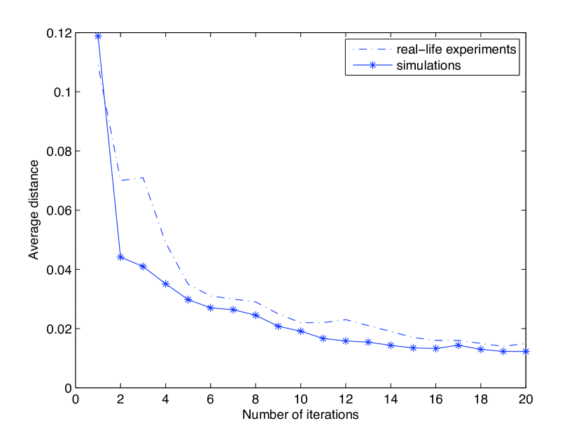
Figure 3: Comparison of the convergence of the Beta Experts algorithm in real-life experiments and in simulations.

7 Conclusions

We have presented a new approach to content-based image retrieval based on multinomial relevance feedback. We model the knowledge of the system using a Dirichlet process as well as Beta Experts algorithm. Both models suggests an algorithm for generating images for presentation that trades exploration and exploitation. We show that the BE approach that assumes that the user has a set of images as their target is a better reflection of user behaviour than the assumption that the user has a single ideal target in their mind. Furthermore, the experiments confirm that the new approach outperforms earlier work using more heuristic strategies.

References

- [1] A. Asuncion, M. Welling, P. Smyth, and Y. W. Teh. On smoothing and inference for topic models. In Proceedings of the International Conference on Uncertainty in Artificial Intelligence, 2009.
- [2] H. Attias. A variational bayesian framework for graphical models. In Proceedings of Neural Information Processing Systems, 2000.
- [3] P. Auer and A. Leung. Relevance feedback models for content-based image retrieval. In Multimedia Analysis, Processing and Communications. Springer, 2009.
- [4] M. J. Beal. Variational algorithms for approximate bayesian inference. PhD Thesis, Gatsby Computational Neurosicence Unit, University College London, 2003.
- [5] O. Chapelle and L. Li. An empirical evaluation of thompson sampling. In Proceedings of Neural Information Processing Systems, volume 25, 2011.
- [6] I. Cox, M. Miller, T. Minka, T. Papathomas, and P. Yianilos. The bayesian image retrieval system, pichunter: theory, implementation, and psychophysical experiments. IEEE Transactions on Image Processing, 9:20 – 37, 2000.
- [7] M. Crosier and L. Griffin. Using basic image features for texture classification. International Journal of Computer Vision, 88(3):447 – 460, 2010.
- [8] R. Datta, D. Joshi, J. Li, and J. Wang. Image retrieval: Ideas, influences, and trends of the new age. ACM Comput. Surv., 2008.
- [9] D. Głowacka, A. Medlar, and J. Shawe-Taylor. Sifting through images with multinomial relevance feedback. In NIPS Workshop Beyond Classification: Machine Learning for Next Generation Computer Vision Challenges, 2010.
- [10] D. Głowacka and J. Shawe-Taylor. Content-based image retrieval with multinomial relevance feedback. In JMLR Workshop and Conference Proceedings: 2nd Asian Conference on Machine Learning, Tokyo, 2010, volume 13, pages 111–125, 2010.
- [11] T. S. Jaakkola. Tutorial on variational approximation methods. In M. Opper and D. Saad, editors, Advances in Mean Field Methods, pages 129 – 159. MIT Press, 2001.
- [12] M. Jordan, Z. Ghahramani, T. S. Jaakkola, and L. K. Saul. An introduction to variational methods for graphical models. In M. Jordan, editor, Learning in Graphical Models, pages 105 – 162. MIT Press, 1999.
- [13] A. Torralba, R. Fergus, and W. Freeman. 80 million tiny images: a large data set for nonparametric object and scene recognition. IEEE Transactions on Pattern Analysis and Machine Intelligence, 30(11):1958 – 1970, 2008.