Shortest path and maximum flow problems in planar flow networks with additive gains and losses

Abstract

In contrast to traditional flow networks, in additive flow networks, to every edge $e$ is assigned a gain factor $g(e)$ which represents the loss or gain of the flow while using edge $e$. Hence, if a flow $f(e)$ enters the edge $e$ and $f(e)$ is less than the designated capacity of $e$, then $f(e)+g(e)\geq 0$ units of flow reach the end point of $e$, provided $e$ is used, i.e., provided $f(e)\neq 0$. In this report we study the maximum flow problem in additive flow networks, which we prove to be NP-hard even when the underlying graphs of additive flow networks are planar. We also investigate the shortest path problem, when to every edge $e$ is assigned a cost value for every unit flow entering edge $e$, which we show to be NP-hard in the strong sense even when the additive flow networks are planar.

1 Introduction

In traditional flow network problems, such as the max-flow problem, it is assumed that if $f(e)$ units of flow enter the edge $e=(v,u)$ at its tail $v$, exactly $f(e)$ units will reach its head $u$. In practice this assumption in many flow models does not hold. For instance, in the well-known generalized flow networks, if $f(e)$ units of flow enter $v$, and a gain factor $g(e)$ is assigned to $e$, then $g(e)\times f(e)$ units reach $u$. Depending on the application, the gain factor can represent the loss or gain due to evaporation, energy dissipation, interest, leakage, toll or etc.

The generalized maximum flow problem has been widely studied. Similar to the standard max-flow problem, generalized max-flow problem can be formulated as a linear programming, and therefore it can be polynomially solved using different approaches such as modified simplex method, or the ellipsoid method, or the interior-point methods. Taking advantage of the structure of the problem, different general purpose linear programming algorithms have been tailored to speed up the calculation of max-flow in generalized flow networks [6, 8, 11].

The strong relationship between generalized max-flow problem and minimum cost flow problem was first recognized and established by Truemper in [15]. Exploiting this relationship and more importantly the discrete structure of the underlying graph, the generalized max-flow problem can also be solved in polynomial time by combinatorial methods [16, 5, 12, 3, 4, 14].

In contrast to the well-studied generalized flow networks, recently in [2], the authors introduced and investigated flow networks where an additive fixed gain factor is assigned to every edge if used. Flow networks with additive gains and losses (additive flow networks for short) have several applications in practice. In communication networks, a fixed-size load is added to every package being sent out by routing nodes in the network. In transportation of goods or commodities, a fixed amount may be lost in the transportation process or a flat-rate amount of other commodities or cost may be added to the commodity passing every toll station. In financial systems there are fixed costs or losses for every transaction.

The max-flow problem in additive networks can be views as the problem of finding a feasible flow which either maximizes the amount of flows departing the source vertices or maximizes the amount of flow reaching the sink vertices (respectively called maximum in-flow and maximum out-flow problems). Similarly, assuming that a unit flow is departing a source vertex, the shortest path problem is the problem of finding a feasible flow along a path from the source vertex to the sink vertex with minimum accumulated cost.

As explained in [2], flow networks with additive gains and losses, are different in many aspects from standard and generalized flow networks due to some properties such as flow discontinuity, lack of max-flow/min-cut duality, and unsuitability of augmented path methods. Similarly, some basic properties of the shortest path in standard flow network do not hold in the additive case. For instance, it is not anymore the case that the sub-path, the prefix or the suffix of a shortest path must themselves be shortest. For more details on the properties of additive flow networks, we refer the reader to [2]. These differences make both the max-flow problem and the shortest path problem hard to solve for additive flow networks. Precisely speaking, the authors of the same paper show that the shortest path problem and the maximum in/out-flow problems are NP-hard for general graphs. In this paper we extend their results to the case where the underlying graph of the flow network is planar.

Organization of the Report.

In Section 2 we give precise formal definitions of several notions regarding the additive flow networks and the corresponding problems. Section 3 concerns the shortest path problem in the additive flow networks; in this section we show that this problem is NP-hard in the strong sense when the underlying graph of the network is planar and Section 4 extends the NP-hardness of maximum in/out-flow problems to planar additive flow networks. Finally, Section 5 is a brief preview of future work.

2 Definitions and preliminaries

A flow network with additive losses and gains (additive flow network for short) is defined by a tuple $N=(V,E,S,T,u,c,g)$, where $G=(V,E)$ is the directed underlying graph with $n=|V|$ vertices and $m=|E|$ edges. The two sets $S,T\subset V$ are respectively the designated set of source and sink vertices. $u:E\rightarrow\mathbb{R}^{+}$ is the edge capacity function, while $c:E\rightarrow\mathbb{R}$ is the cost function and $g:E\rightarrow\mathbb{R}$ assigns a gain or loss value to every edge if used. Precisely speaking, the cost $c(e)$ per units of flow and the gain factor $g(e)$ are applied, only if a positive flow enters the edge $e$.

Definition 1 (Incoming and outgoing edges).

Consider the directed graph $G=(V,E)$ and $v\in V$. Two functions $in:V\rightarrow 2^{E}$ and $out:V\rightarrow 2^{E}$ respectively represent the set of incoming edges and the set of outgoing edges for every vertex. Formally, for every $v\in V$:

$$in(v)=\{e|e=(u,v)\in E\},$$

$$out(v)=\{e|e=(v,u)\in E\}.$$

Similarly the indegree and outdegree functions for every vertex $v\in V$ are respectively defined as $deg^{+}(v)=|\,in(v)\,|$ and $deg^{-}(v)=|\,out(v)\,|$. $\square$

As in traditional flow networks, it is assumed that for every source vertex $s\in S$, $deg^{+}(s)=0$ and for every sink vertex $t\in T$, $deg^{-}(t)=0$. Flow $f:E\rightarrow\mathbb{R}^{+}$ in a network $N$ is feasible if it satisfies edge capacity $0\leq f(e)\leq u(e)$ for every edge $e\in E$ and flow conservation constraint at every vertex in $V$. Formally speaking, $f$ satisfies the flow conservation constraints if for every $v\in V-(S\uplus T)$:

$$\sum_{e\in in(v),f(e)>0}\max(0,f(e)+g(e))=\sum_{e\in out(v)}f(e).$$

Given edge $e=(v,u)$, if flow $f(e)$ exits vertex $v$, then $\max(0,f(e)+g(e))$ units reach $u$. Therefore edge $e=(u,v)\in E$ is lossy if the entering edge $f(e)$ is positive and $g(e)<0$. Edge $e$ consumes the entering flow if $f(e)+g(e)<0$, in which case no flow reaches the vertex $v$.

Definition 2 (Out-flow and in-flow).

Given flow $f$ for network $N$, the out-flow is the summation of the amount of flow exiting source vertices, i.e., $f_{out}=\sum_{s\in S,e\in out(s)}f(e)$. Similarly, in-flow is the summation of flow values entering all sink vertices, namely $f_{in}=\sum_{t\in T,e\in in(t),f(e)>0,}max(0,f(e)+g(e))$. $\square$

In additive flow networks, the max-flow problem can be studied from the producers’ (source vertices) point of view or from the consumers’ (sink vertices) point of view. Hence, the maximum out-flow problem is the problem of finding a feasible flow $f$ maximizing $f_{out}$, and the maximum in-flow problem is defined similarly. Regarding these two problems, while trying to maximize the amount of outgoing/incoming flows, we are not concerned with the cost of flow.

On the other hand, in additive flow networks, the shortest path problem can be generalized in several ways. For instance, given a producer vertex $s\in S$ (similarly consumer vertex $t\in T$), the problem can be defined as finding a consumer vertex $t\in T$ (producer vertex $s\in S$) with the shortest distance among the others, with respect to the cost of a unit flow departing $s$ towards $t$. A more generalized variation of the problem can be defined, where neither of the source or destination vertices are fixed. Therefore, the generalized shortest path is the problem of finding a source vertex $s\in S$, a destination vertex $t\in T$, and a path $\Pi$ from $s$ to $t$ with minimum cost, if a unit of flow departs $s$. Without loss of generality, in the rest of this report, it is assumed that the sets of source and sink vertices each has one member (namely $|S|=|T|=1$). Hence, every negative result shown for this special case is immediately applicable to the generalized version of the shortest path problem. Section 3 concerns the shortest path problem and the related definitions with more details.

Definition 3 (Cost of flow).

Given a flow function $f$ in network $N$, the cost of flow on every edge $e$ is $f(e)\times c(e)$. Similarly the accumulated cost of $f$ is the summation of cost of flow entering all edges, i.e., $cost(f)=\sum_{e\in E}f(e)\times c(e)$. $\square$

Example 4.

In Figure 1 an additive flow network and a feasible flow from vertex $s$ to vertex $t$ are depicted. The cost of unit flow for every edge is $1$ and the capacity of every edge is $B+1$ for $B>1$. For a compact illustration of figures in this report, we adopt the following conventions:

• If we label an edge $e$ with $g=r$ or $c=r$ or $u=r$, for some $r\in\mathbb{R}$, then we mean that $g(e)=r$ or $c(e)=r$ or $u(e)=r$, respectively.

• If we omit such a label on an edge $e$, then we mean that the value of the corresponding function for $e$ is the default value (as stated in the description of that figure).

For instance in Figure 1, $g((s,v_{1}))=B+1$ for edge $(s,v_{1})$, is represented by $g=B+1$ by that edge. The missing gain values are the default value $0$. In this example, the initial unit flow leaves vertex $s$ while $B+2$ units reach $v_{1}$, due to gain value $B+1$ assigned to edge $(s,v_{1})$. The flow entering edge $(v_{1},v_{5})$ is fully absorbed by the gain factor $-B$ assigned to it. Hence, the accumulated cost of the flow along path $\Pi=(s,v_{1},v_{2},v_{3},t)$ is $B+4$ while the accumulated cost of the flow $f$ is $B+5$.

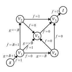
Figure 1: An example of an additive flow network $N$ and the flow function $f$ assigning feasible flow values to every edge of $N$. Missing gain values are $0$, the cost function $c$ is $1$ on every edge, and the capacity function $u$ is a ”large number” on every edge (for example $B+1$).

$\square$

3 Shortest path problem in additive flow network

Let $N$ be an additive flow network and let $\Pi=\bigl{(}(s,v_{1}),(v_{1},v_{2}),\ldots,(v_{k-1},t)\bigl{)}$ be a (simple) path in $N$ from vertex $s$ to $t$. Let $e_{i}=(v_{i-1},v_{i})$ for $2\leq i\leq k-1$ while $e_{1}=(s,v_{1})$ and $e_{k}=(v_{k-1},t)$. Given the flow $f$ along path $\Pi$ with the initial flow $f_{1}$ entering $e_{1}$ (seed flow for short), the accumulated flow entering edge $e_{i}$ for every $1\leq i\leq k$, is represented by:

$$\gamma(\Pi,f_{1},i)=f_{1}+\sum_{j<i}g(e_{1}).$$

Definition 5 (Feasible and dead-end flows along a path).

Flow $f$ with the seed flow $f_{1}$, is feasible along path $\Pi=(e_{1},\ldots,e_{k})$ if the flow on every edge is positive and a positive amount of flow reaches the destination $t$. i.e. for $1\leq i\leq k+1$:

$$\gamma(\Pi,f_{1},i)>0.$$

Flow $f$ is infeasible or dead-end if an edge $e_{i}$ for $1\leq i\leq k$ absorbs all the entering flow, due to the loss value $g(e_{i})$ assigned to that edge. Hence, no flow reaches the destination vertex. $\square$

For every vertex $t$ reachable from $s$ via some path $\Pi$, there exists a threshold value $T$ such that a flow along $\Pi$ is feasible only if its seed flow $f_{1}>T$. Finding the reachability threshold (if exists) for every pair of source and sink vertices is a polynomial task, as formally stated in Lemma 6.

Lemma 6.

Consider a flow network $N=(V,E,\{s\},\{t\},u,c,g)$. There exists a polynomial time algorithm that decides the reachability of $t$ from $s$ in network $N$ and finds the reachability threshold in ${\cal O}\bigl{(}nm\bigr{)}$, if such threshold exists.

Proof.

In order to find the threshold value $T$ in $N$ such that at least one path from source $s$ to destination $t$ is feasible (i.e., $t$ is reachable from $s$ for seed flow $f_{1}>T$), one can use a variation of well-known shortest path algorithms (such as Bellman-Ford algorithm) in the reversed graph of $N$. The reversed graph is constructed from the underlying graph of $N$ by reversing the direction of every edge $e$ and assigning $-g(e)$ as the weight of the reversed edge. Hence, the reachability threshold problem reduces to a modified variation of the shortest path problem from $t$ to $s$. This problem is a modified variation of the traditional shortest path problem with negative costs, in the sense that the distance of no two vertices can be negative. Hence, in the modified variation of the Bellman-Ford algorithm in the process of updating the distance matrix for every vertex $v$ from $s$, the distance of $v$ from $s$ is set to $\max\{0,d\}$, where $d$ is the newly updated distance of $v$ from $s$. Note that due to flow conservation constraints at every vertex, there is no feasible flow with positive gain cycles involved in it. Also in this modified variation of Bellman-Ford algorithm the distance of no two vertices can be negative. Assuming that there is no positive gain cycle in $N$, means that there is no negative cycle in the reversed graph, which in turn implies that the modified variation of Bellman-Ford algorithm always returns the threshold, if $t$ is reachable from $s$. The correctness proof of this approach is straightforward and similar to the proof of the correctness of the standard Bellman-Ford algorithm for the shortest path problem. The time complexity of this algorithm is the same as the standard Bellman-Ford algorithm, which has ${\cal O}\bigl{(}|V|\times|E|\bigr{)}$ worst case time bound. ∎

The accumulated cost of a flow along the path $\Pi=(e_{1},\ldots,e_{k})$ (feasible or not), is the summation of the cost of the flows entering every edge times the value of cost function assigned to that edge, namely:

$$\sum_{1\leq i\leq k}c(e_{i})\gamma(\Pi,f_{1},i).$$

In [2] regarding the shortest path problem, the authors simplify the problem by assuming that the seed value $f_{1}=1$. On the other hand, given the source and destination vertices $s$ and $t$ in flow network $N$, it may be the case that for every path $\Pi$ from $s$ to $t$, no feasible flow along $\Pi$ with the seed value $f_{1}=1$ exists. Accordingly the definition of shortest path problem in [2] can be generalized as in following.

Definition 7 (Shortest path in additive flow networks).

The shortest path problem in additive flow network $N$ for a given pair of source and sink vertices $\{s,t\}$, is the problem of finding a min-cost feasible flow along some path $\Pi$ from $s$ to $t$, when the seed flow $f_{1}=\min\{1,T\}$. Where $T$ is the reachability threshold for the source/destination pair $\{s,t\}$. $\square$

In contrast to the shortest path problem in traditional flow networks, this problem is hard in the case of additive flow networks. From Theorem 1 in [2] it can be inferred that when the underlying graph of the flow network is planar, this problem is weakly NP-hard. In other words, the problem may be polynomially solvable if the cost and capacity values assigned to the edges are bounded from above by some polynomial function in the size of the graph. In the same paper it is shown that this result holds if the cost and gain values are all nonnegative integers, even for the case where the underlying graph is not necessary planar.

In this section we show that the shortest path problem is NP-hard in the strong sense when the underlying graph of the additive flow network is planar (planar additive flow network for short). We show this result using a polynomial reduction from a problem called Path Avoiding Forbidden Transitions (PAFT for short) [7]. PAFT is a special case of the problem of finding a path from source vertex $s$ to destination vertex $t$ while avoiding a set of forbidden paths (initially introduced in [17]). Before presenting the main result of this section (as stated in Theorem 13), we briefly define PAFT and some results on this problem (for more details, the reader is referred to [7]).

Given undirected multi-graph $G=(V,E)$, a transition in $G$ is an unordered set of two distinct edges of $E$ which are incident to the same vertex of $V$. If $\mathcal{T}$ denotes the set of all possible transitions in the graph $G$, the set $\mathcal{F}$ of forbidden transitions is a subset of $\mathcal{T}$. Then $\mathcal{A}=\mathcal{T}-\mathcal{F}$ denotes the set of allowed transitions. A simple path $\Pi=(e_{1},e_{2},\ldots,e_{k})$, where $e_{1}=\{s,v_{1}\}$ and $e_{k}=\{v_{k-1},t\}$, is $\mathcal{F}$-valid if for every $1\leq i<k$, $\{e_{i},e_{i+1}\}\notin\mathcal{F}$; namely, no transition in $\Pi$ is forbidden. A vertex $v$ is involved in a forbidden transition $\{e,e^{\prime}\}$ if two edges $e$ and $e^{\prime}$ share $v$ and $\{e,e^{\prime}\}\in\mathcal{F}$.

Definition 8 (PAFT).

Consider a multi-graph $G=(V,E)$, a set of forbidden transitions $\mathcal{F}$ and designated source and destination vertices $s,t\in V$. PAFT is the problem of find an $\mathcal{F}$-valid path from $s$ to $t$, if exists. $\square$

Lemma 9.

PAFT is NP-complete for planar graphs where the degree of every vertex $v\in V-\{s,t\}$ is $3$ or $4$, where $s$ and $t$ are the source and destination vertices, respectively.

Proof.

In [7], the authors show that PAFT is NP-complete in planar graphs where the degree of every vertex is at most $4$. Consider graph $G=(V,E)$ with maximum vertex degree $4$ and source and destination vertices $s$ and $t$, and let $\mathcal{F}$ be the set of forbidden transitions. Graph $G^{\prime}=(V^{\prime},E^{\prime})$ and the set of forbidden transitions $\mathcal{F}^{\prime}$ are constructed as explained in what follows.

Initially $V^{\prime}=V$, $E^{\prime}=E$ and $\mathcal{T}^{\prime}=\mathcal{T}$. Until there is no vertex of degree $1$ or $2$, for every vertex $v\in V^{\prime}-\{s,t\}$:

1. If $deg(v)=1$: (i) $V^{\prime}=V^{\prime}-{v}$, (ii) $E^{\prime}=E^{\prime}-e$, where $e$ is the edge incident to $v$, and (iii) $\mathcal{T}^{\prime}=\mathcal{T}^{\prime}-\tau$, for every forbidden transition $\tau$ that $v$ is involved in.

2. If $deg(v)=2$ and $\tau=\{e_{1},e_{2}\}\in\mathcal{F}$, where $e_{1}$ and $e_{2}$ share $v$: (i) $V^{\prime}=V^{\prime}-{v}$, (ii) $E^{\prime}=E^{\prime}-\{e_{1},e_{2}\}$, and (iii) $\mathcal{T}^{\prime}=\mathcal{T}^{\prime}-\tau$

3. If $deg(v)=2$ and $\tau=\{e_{1},e_{2}\}\notin\mathcal{F}$, where $e_{1}$ and $e_{2}$ share $v$: (i) $v$ is smoothed out by removing $v$ and the two incident edge $e_{1}=\{w,v\}$ and $e_{2}=\{v,u\}$ and introducing a new edge $e^{\prime}=\{w,u\}$. (ii) For $i\in\{1,2\}$ if $\{e_{i},e\}\in\mathcal{F}$ for some $e\in E$; $F^{\prime}=F^{\prime}\uplus\{\{e^{\prime},e\}\}-\{e_{i},e\}$.

It is straightforward and left to reader to verify that there is $\mathcal{F}$-valid path from $s$ to $t$ in $G$ iff there is a $\mathcal{F^{\prime}}$-valid path from $s$ to $t$ in $G^{\prime}$. Accordingly, the NP-hardness of PAFT for planar graphs with maximum degree $4$ results in the NP-hardness of PAFT for the class of planar graphs where the degree of every vertex is $3$ or $4$. In [7], using a similar approach, this result is extended to grid graphs. ∎

This lemma helps us to draw the main result of this section (as stated at the end of this section in Theorem 13). Before that, in an intermediate step, Procedure 10 represents an approach to transforming an instance of PAFT into an additive flow network. Without loss of generality, we assume that the source and the sink vertices are not involved in any forbidden transition.

Procedure 10 (PAFT’s instance into additive flow network).

Consider a planar undirected multi-graph $G=(V,E)$, a set of forbidden transitions $\mathcal{F}$, and source and destination vertices $s$ and $t$ as an instance of PAFT, where for every vertex $v\in V$, $deg(v)\in\{3,4\}$. We transform such instance of PAFT into an additive flow network $N$ in several steps:

1. Every undirected edge $e=\{v,u\}$ is replaced by a pair of parallel incoming/outgoing directed edges $e=(v,u)$ and $e^{\prime}=(u,v)$.

2. Two new vertices $s^{\prime}$ and $t^{\prime}$ are introduced. $s^{\prime}$ is connected to $s$ via edge $e_{s}=(s^{\prime},s)$ and $t$ is connected to $t^{\prime}$ via $e_{t}=(t,t^{\prime})$. $e_{t}$ has $0$ gain while $e_{s}$ has gain value $B$ assigned to it for some $B>1$. To both edges $e_{s}$ and $e_{t}$ is assigned cost value $0$.

3. For every vertex $v$, not involved in any forbidden transition, every outgoing edge $(v,v^{\prime})$ is subdivided into two edges $(v,w)$ and $(w,v^{\prime})$ by introducing a new vertex $w$. Two edges $(v,w)$ and $(w,v^{\prime})$ respectively have gain value $-B$ and $+B$ and cost $c=+B$ and $c=-B$. Figure 2 represents the replacement gadget for a vertex $v$ with degree $4$.

   The gain value $-B$ assigned to every outgoing edge $(v,w)$ guarantees that if $B+1$ units of flow enter the gadget of $v$, the exiting flow reaches the gadget of at most one of the neighbors of $v$ in $G$. The gain value $+B$ assigned to the edge $(w,v^{\prime})$ (connected to outgoing edge $(v,w)$) compensates for the lost flow that enters $(v,w)$, if some flow reach $w$. Hence, $B+1$ units of flow entering the gadget of $v$ reach the gadget of exactly one of the neighbors of $v$ in $G$ with no loss, if only one of the outgoing edges is chosen.

   Moreover based on the same reasoning, the cost values in this gadget assure us that the $B+1$ units of flow entering this gadget reaches the gadget of the neighboring vertex with no cost, if only one of the outgoing edges is chosen.

   In summary, if $B+1$ units of flow enter such gadget of a vertex $v$, in order to have some flow reaching the neighboring gadget, one of the outgoing edges must have $B+1-x$ units entering flow for $0\leq x<1$. In this case $B+1-x$ units reach the neighboring gadget and the $x$ units of flow is consumed with total cost $xB$.

   

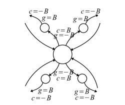
   Figure 2: The gadget that replaces a vertex of degree $4$ which is not involved in any forbidden transition.

4. Consider vertex $v$ involved in some forbidden transitions with degree $d=deg(v)\leq 4$ incident to $d$ pairs of incoming/outgoing parallel edges $\{e_{1},e_{1}^{\prime}\},\ldots,\{e_{d},e_{d}^{\prime}\}$. Originally in graph $G$ vertex $v$ is incident to $e_{1},\ldots,e_{d}$. The planar embedding of $v$ in $G$ is represented in Figure 3 on the left, when $d=4$.

   1. If $d=3$: vertex $v$ is replaced by $3$ new vertices $v_{1},v_{2},v_{3}$ where $v_{i}$ is incident to the pair $\{e_{i},e_{i}^{\prime}\}$ for $1\leq i\leq 3$, based on the planar embedding of edges $e_{1},e_{2},e_{3}$ in $G$. For $1\leq i,j\leq 3$, two vertices $v_{i}$ and $v_{j}$ are directly connected with a pair of parallel incoming/outgoing edges, if $\{e_{i},e_{j}\}\notin\mathcal{F}$. The cost of every edge is $0$ and the gain factor for every introduced edge $(v_{i},v_{j})$ is $-B$ for $1\leq i,j\leq 3$. Finally, every outgoing edge connecting $v_{i}$ (for $1\leq i\leq 3$) to another gadget (corresponding to one of the neighbors of $v$ in $G$) has cost $0$ and gain factor $+B$.

   2. If $d=4$ and $\{\{e_{1},e_{4}\},\{e_{2},e_{3}\}\}\nsubseteq\mathcal{A}$: A gadget of four vertices replaces $v$, following the same procedure as explained in the previous case. Figure 3 depicts an example of transforming a vertex of degree $4$ involved in some forbidden transitions.

      

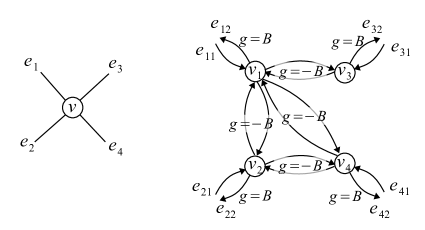
      Figure 3: On the left is the planar embedding of a vertex $v\in V$ incident to $4$ edges where $\{e_{2},e_{3}\},\{e_{3},e_{4}\}\in\mathcal{F}$. The right image shows the gadget replacing vertex $v$. Every edge connecting two vertices $v_{i}$ and $v_{j}$ for $1\leq i,j\leq 4$ has cost value $0$ and gain value $-B$ assigned to it. Vertices $v_{2}$ and $v_{3}$ are not directly connected since their corresponding edges $e_{2}$ and $e_{3}$ are involved in a forbidden transition. Hence, a flow from $v_{2}$ to $v_{3}$ (and vice versa) loses $-2B$ units. Same situation holds for $v_{3}$ and $v_{4}$.

   3. If $d=4$ and $\{\{e_{1},e_{4}\},\{e_{2},e_{3}\}\}\subseteq\mathcal{A}$: Using the same approach as in the previous case spoils the planarity of the resulting network $N$. To solve this problem, vertex $v$ is replaced by a gadget of $5$ vertices. In addition to $4$ vertices $v_{1},\ldots,v_{4}$, where for $1\leq i\leq 4$, $v_{i}$ is connected to the pair of incoming/outgoing edges $\{e_{i},e_{i}^{\prime}\}$, a central vertex $w$ is introduced as well. As depicted in Figure 4, in the replacing gadget, vertices $v_{1}$ and $v_{4}$ (also vertices $v_{2}$ and $v_{3}$) are connected via the central vertex $w$. Any other two vertices $v_{i}$ and $v_{j}$ for $1\leq i,j\leq 4$ are directly connected via a pair of parallel incoming/outgoing edges, if $\{e_{i},e_{j}\}\notin\mathcal{F}$ (with gain and cost values $-B$ and $0$ respectively). The cost and gain factors for every edge can be found by that edge and the missing values are the default value $0$.

      Assume $B+1$ units of flow reach any of the four vertices $v_{1},\ldots,v_{4}$. The gain and cost values assigned to the edges incident to $w$ guarantee that a flow can go through the central vertex $w$ with no cost and reach the destination with $-B$ units loss, only if it is from $v_{1}$ to $v_{4}$ and vice versa or if it is from $v_{2}$ to $v_{3}$ and vice versa. Any other flow, with the initial value $B+1$ units, that uses $w$ is either costly (costs $2B(B+1)$) or gets fully consumed (i.e., does not reach the destination).

5. Every edge has capacity $B+1$.

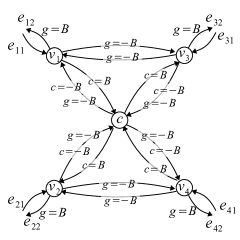
Figure 4: The gadget replacing vertex $v$ where $deg(v)=4$ and $\{e_{1},e_{4}\},\{e_{2},e_{3}\}\in\mathcal{A}$. Edges $e_{1},\ldots,e_{4}$ are the edges connected to $v$ as represented in a planar embedding of $G$ in Figure 3 (on the left). This gadget replaces $v$ where $\{e_{1},e_{2}\},\{e_{3},e_{4}\}\in\mathcal{F}$.

Note that if the undirected multi-graph $G$ is planar, then so is the underlying graph of the flow network $N$ as a result of the preceding transformation. Also since the capacity of every edge is $B+1$, it is guaranteed that maximum amount of flow that enters a gadget is $B+1$ units and no more than $B+1$ units of flow departs any gadget. $\square$

Example 11.

Figure 5(a) denotes a graph $G$ and its designated source and destination vertices. The set of forbidden transitions is $\mathcal{F}=\{\{e_{2},e_{3}\},\{e_{3},e_{4}\}\}$. Figure 5(b) shows the additive flow network $N$ constructed based on $G$ and the set of forbidden transitions. The set of four vertices shown in the dashed circle represents the gadget replacing vertex $v$ which is the only vertex involved in the forbidden transitions. The missing gains of every edge in this gadget is $-B$.

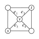
(a) Graph $G$, input for PAFT.

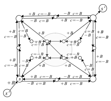
(b) Additive flow network $N$.

Figure 5: Additive flow network $N$ in 5(b), constructed based on the graph $G$ in 5(a) and the set of forbidden transitions $\mathcal{F}=\{\{e_{2},e_{3}\},\{e_{3},e_{4}\}\}$. The set of four vertices shown in the dashed circle represent the gadget replacing middle vertex $v$. The missing gain values for every edge in this gadget are $-B$. The gain of every other edge is shown by $+B$ or $-B$ by that edge. The default values for missing cost and capacity functions are respectively $0$ and $B+1$.

$\square$

Lemma 12.

Consider an undirected multi-graph $G$, a set of forbidden transitions $\mathcal{F}$, and source and destination vertices $s$ and $t$ as an instance of PAFT, where the degree of every vertex $v\in V$ is $3$ or $4$. Let $N$ be the additive flow network constructed from $G$ and the forbidden transitions set $\mathcal{F}$ using Procedure 10. There is a (simple) $\mathcal{F}$-valid path from $s$ to $t$ iff there exists a feasible flow in $N$ along a (simple) path from $s^{\prime}$ to $t^{\prime}$ with no cost, when seed flow $f_{1}=1$.

Proof.

($\Rightarrow$) Assume there is a $\mathcal{F}$-valid (simple) path $\Pi=(s,v_{1},\ldots,v_{k},t)$ in $G$. Based on $\Pi$ we suggest a flow in $N$ where a unit of flow departing $s^{\prime}$ reaches the gadget of $v_{1}=s$ while gaining $B$ units of flow. The accumulated cost so far is $0$. Based on the construction of every gadget, following the path $\Pi$, the $B+1$ units of flow can go through the corresponding gadget of every vertex $v_{i}$ and reach the gadget of $t$ with no loss and no cost. Therefore, there is a feasible flow in $N$ from $s^{\prime}$ to $t^{\prime}$ with $0$ cost.

($\Leftarrow$) Let $f$ be a feasible flow in $N$ along a (simple) path $\Pi=(s^{\prime},s,\ldots,t,t^{\prime})$ with no cost, where seed flow $f_{1}=1$. Based on the construction of $N$ from $G$, in a coarser view, a feasible flow goes from one gadget to another gadget. Hence, path $\Pi$ can be viewed as $\Pi=(s^{\prime},\underline{s},\underline{v_{1}},\ldots,\underline{v_{k}},\underline{t},t^{\prime})$, where $\underline{v_{i}}$ represent the gadget corresponding to vertex $v_{i}$ that some of its edges are used in path $\Pi$.

The unit flow departs $s^{\prime}$ and $B+1$ units reach the gadget $\underline{s}$ with cost $0$. When $B+1$ units reach the gadget $\underline{v}$ of $v$:

• If $v$ is not involved in any forbidden transition: As explained in the third step of Procedure 10, $B+1-x$ units reach the gadget of one of the neighbors of $v$ with cost $xB$ for $0\leq x<1$.

• If $v$ is involved in some forbidden transitions:

  • If $v$ is an instance of $4$-(a) or $4$-(b) in Procedure 10, flow can reach the gadget of exactly one of neighbors of $v$ only if no forbidden transition is used.

  • If $v$ is an instance of $4$-(c) in Procedure 10, as explained in this case, the flow is either fully consumed or suffers cost $2B(B+1)$, if any forbidden transition is used. The entering flow to this gadget reaches the neighboring gadget with no loss and no cost, only if no forbidden transition is used by the flow.

  • For every gadget involved in some forbidden transitions, it is always the case that the entering $B+1$ units of flow either is fully consumed or suffers no loss upon reaching the neighboring gadget.

Every feasible flow $f$ originated from $s^{\prime}$ with seed flow $f_{1}=1$ as reaches $t^{\prime}$ has gained $B-x$ units, with accumulated cost $xB$ for $0\leq x<1$, if no forbidden transition is used. On the other hand, if any forbidden transition is used, a feasible flow along a path from $s^{\prime}$ to $t^{\prime}$ costs at least $2B(B+1)$, as explained in the sub-cases of case $4$ in Procedure 10. Accordingly, a feasible flow with $f_{1}=1$ along some path from $s^{\prime}$ to $t^{\prime}$ has minimum cost $0$, only if no forbidden transition is used and $x=0$ (i.e., $B+1$ units reach $t^{\prime}$ with no loss). ∎

The following theorem concludes this section.

Theorem 13.

The simple shortest path problem is NP-hard in the strong sense for additive flow networks where the underlying graph is planar.

Proof.

Proof is immediate based on Lemmas 9 and 12 and the fact that the procedure 10 can be carried out in polynomial time (with respect to the size of the input graph $G$ and the set of forbidden transitions $\mathcal{F}$). ∎

4 Maximum flow problem in additive flow network

In [2], the authors study the problem of maximum flow with additive gains and losses for general graphs. They show that finding maximum in-flow and out-flow are NP-hard tasks for general graphs. In this section we show the same result for planar additive flow networks. In order to show this result, we facilitate a special variation of planar satisfiability problem (planar SAT), which is briefly defined in the following.

Definition 14 (Strongly planar CNF).

Conjunctive normal form (CNF for short) formula $\varphi=(\mathcal{X},\mathcal{C})$ with the set of variable $\mathcal{X}$ and the set of clauses $\mathcal{C}$ is strongly planar if graph $G_{\varphi}=(V,E)$ constructed as follows is planar:

1. $V$ contains a vertex for every literal and one vertex for every clause.

2. $\{x,\widetilde{x}\}\in E$ for every $x\in\mathcal{X}$, where $\widetilde{x}$ denotes the negation of boolean variable $x$.

3. If a claus $C$ contains literal $\overline{x}$ (which can be $x$ or $\widetilde{x}$), there is an edge $\{\overline{x},C\}$ connecting vertex $\overline{x}$ and the vertex corresponding to $C$.

4. No other edge exists other than those introduced in Part $2$ and Part $3$.

$\square$

Example 15.

Consider CNF formula $\varphi=(\widetilde{x}\vee y\vee\widetilde{z})\wedge(x\vee\widetilde{y}\vee z)\wedge(x\vee w\vee z)\wedge(\widetilde{x}\vee\widetilde{w}\vee\widetilde{z})$. Figure 6 represents a planar embedding of the graph $G_{\varphi}$.

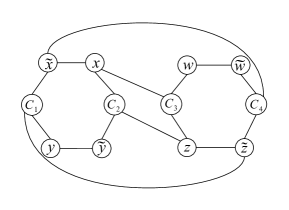
Figure 6: Underlying graph of the 3CNF formula $\varphi=(\widetilde{x}\vee y\vee\widetilde{z})\wedge(x\vee\widetilde{y}\vee z)\wedge(x\vee w\vee z)\wedge(\widetilde{x}\vee\widetilde{w}\vee\widetilde{z})$.

$\square$

Definition 16 (1-in-3SAT).

Given 3CNF formula $\varphi$, 1-in-3SAT is the problem of finding a satisfying assignment such that in each clause, exactly one of the three literals is assigned to $1$. $\square$

Lemma 17.

Strongly Planar 1-in-3SAT is NP-complete.

For the proof of Lemma 17, we refer the reader to [18]. We use Lemma 17 to present the main contribution of this section (stated in Theorems 21 and 23). Initially, Procedure 18 shows three steps in order to transform a CNF formula $\varphi$ into an additive flow network $N_{\varphi}$.

Procedure 18 (CNF into additive flow network).

Consider graph $G_{\varphi}=(V,E)$ corresponding to a 3CNF $\varphi$ as an instance of 1-in-3SAT. Starting from the undirected graph $G_{\varphi}$, additive flow network $N_{\varphi}$ is constructed using the following steps:

1. Every undirected edge $\{\overline{x},C\}$ connecting literal $\overline{x}$ (which can be $x$ or $\widetilde{x}$) to clause $C$ is replaced by a directed edge $e=(x,C)$ from $x$ to $C$ where $u(e)=1$ and $g(e)=0$.

2. For every clause-vertex $C_{i}$, a sink vertex $t_{i}$ and an edge $e=(C_{i},t_{i})$ are introduced, where $u(e)=1$ and $g(e)=0$.

3. Every pair of literal-vertices $\{x,\widetilde{x}\}$ is replaced by a gadget as shown in Figure 7.

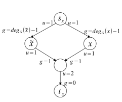
Figure 7: The gadget that replaces every pair of literal-vertices $\{x,\widetilde{x}\}$. The upper bound and the gain or loss of every edge can be found by that edge, where $deg_{G}(x)$ is the degree of literal-vertex $x$ in the graph $G_{\varphi}$. The gadget of every pair $\{x,\widetilde{x}\}$ introduces one source $s_{x}$ and one sink vertex $t_{x}$.

$\square$

Example 19.

The flow network corresponding to the CNF formula $\varphi$ of example 15 is depicted in figure 8. The missing capacity values and gain factors are $1$ and $0$, respectively. For simplicity some source vertices (also some sink vertices) are combined. It is easy to see that the graph of the constructed network $N_{\varphi}$ is planar iff $G_{\varphi}$ is planar.

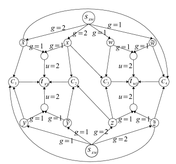
Figure 8: The flow network constructed from the graph $G_{\varphi}$ of CNF formula $\varphi=(\widetilde{x}\vee y\vee\widetilde{z})\wedge(x\vee\widetilde{y}\vee z)\wedge(x\vee w\vee z)\wedge(\widetilde{x}\vee\widetilde{w}\vee\widetilde{z})$.

$\square$

Lemma 20.

CNF formula $\varphi=(\mathcal{X},\mathcal{C})$ is a positive instance of strongly planar 1-in-3SAT iff the maximum in-flow in additive flow network $N_{\varphi}$ is $2|\mathcal{X}|+|\mathcal{C}|$, where $N_{\varphi}$ is constructed according to procedure 18.

Proof.

($\Rightarrow$) Consider a satisfying assignment of variables that every clause has exactly one literal with value $1$. For every literal $\overline{x}$ assigned to $1$ we push $1$ unit flow through the edge connecting a source vertex to the related literal-vertex of $\overline{x}$. The amount of flow that reaches $\overline{x}$ is exactly one unit more than the number of clauses containing $\overline{x}$. This flow saturates all the edge connecting $\overline{x}$ to the vertices of the clauses that contain the literal $\overline{x}$. The remaining one unit flow reaches the sink vertex in the gadget containing the vertex of $\overline{x}$ (plus an extra unit flow gained). Every edge connecting a source to the vertices corresponding to the literals that are assigned $0$, will not be used. It is easy to check that the suggested flow is feasible and all the edges connected to sink vertices are saturated.

($\Leftarrow$) We produce a variable assignment for $\varphi$ based on a given feasible $f$ for $N_{\varphi}$. According to the construction of the gadgets for every pair of literals $\{x,\widetilde{x}\}$ in Figure 7, in every feasible flow at most one of the two edges $(s_{x},x)$ and $(s_{x},\widetilde{x})$ can be used (i.e. in every feasible flow $f$, for every $x\in X$, $f(x)=0\text{ or }f(\widetilde{x})=0$). A literal $\overline{x}$ is set to $1$ if $f((s_{x},\overline{x}))>0$, and is set to $0$ otherwise.

Hence, given $N_{\varphi}$ where $f_{in}=2|\mathcal{X}|+|\mathcal{C}|$, all the edges reaching a sink vertex are saturated. Namely: (i) every edge connecting a clause-vertex to a sink vertex is saturated, which make up $|\mathcal{C}|$ units of flow (i.e. corresponding clause is satisfied) and (ii) the remaining $2|\mathcal{X}|$ units of flow is supplied by the sink vertices of all the gadgets (i.e. $f((s_{x},x))=1$ or $f((s_{x},\widetilde{x}))=1$ for every pair $\{x,\widetilde{x}\}$). Accordingly, if a feasible flow has maximum in-flow $2|\mathcal{X}|+|\mathcal{C}|$, it is the case that for every variable $x$ only one of the literal-vertices $x$ or $\widetilde{x}$ has entering flow, hence in the suggested assignment that literal is set to $1$. Also for every clause $C_{i}$ one unit flow reaches its corresponding vertex, which means that clause is satisfied and only one of its literal is set to $1$. ∎

It is not hard to check that Procedure 18 can be done in polynomial time in the size of the input CNF formula. Hence, based on Lemmas 17 and 20, the following theorem can be deduced immediately.

Theorem 21.

computing a feasible flow $f$ with maximum in-flow $f_{in}$ is an NP-hard problem in the strong for the class planar additive flow networks.

In the context of max-flow problem, for every additive flow network $N=(V,E,S,T,u,g)$ there exists a reversed flow network $N^{\prime}=(V^{\prime},E^{\prime},S^{\prime},T^{\prime},u^{\prime},g^{\prime})$, constructed by reversing the direction of every edge and swapping source vertices with sink vertices (i.e. $S^{\prime}=T$ and $T^{\prime}=S$). Given edge $e=(v,u)$ in $E$, we have $e^{\prime}=(u,v)\in E^{\prime}$ where $u^{\prime}(e^{\prime})=u(e)+g(e)$ and $g(e^{\prime})=-g(e)$. Hence, if edge $e$ is gainy (lossy) in $N$, $e^{\prime}$ is lossy (gainy) in $N^{\prime}$.

Based on the definition of reversed flow networks, the following lemma is straightforward and the details can be found in [2].

Lemma 22.

Consider the feasible flow $f$ for an additive flow network $N$, where for every edge $e,g(e)\geq 0$ (in other words, there is no lossy edge in $N$). Then exists a flow $f^{\prime}$ for the reversed network $N^{\prime}$, where $f_{out}^{\prime}=f_{in}$ (and similarly $f_{in}^{\prime}=f_{out}$).

In the construction of $N_{\varphi}$ from $G_{\varphi}$ based on Procedure 18, there is no lossy edge. Hence the following theorem, as an immediate result of lemma 22, concludes this section. The proof is straightforward and left to the reader.

Theorem 23.

In planar additive flow networks, finding feasible flow $f$ with maximum out-flow $f_{out}$ is an NP-hard problem in the strong sense.

5 Conclusion and future work

In this report we investigated the max-flow and shortest path problems for flow networks with additive gains and losts when the underlying graph is planar. In Sections 3 and 4, we show that both problems are NP-hard in the strong sense for planar additive flow networks, i.e. even when all the values of cost, gain and capacity functions assigned to every edge are bounded by polynomials in the size of the input network.

Hence, there is the question of existence of approximation algorithms for any of the two problems. To our best knowledge, no approximation algorithm has yet been suggested for any of those problems for additive flow networks (with or without any restriction on the structure of the underlying graph).

The other question to investigate is the existence of polynomial time algorithms when some input parameters are fixed. For instance, based on the notion of outerplanarity, every planar graph is $k$-outerplanar for some integer $k\geq 1$. In [1, 13, 10] the authors introduce and study a compositional framework for the analysis of flow networks (based on a so-called Theory of Network Typings); based on this framework in [9], a linear time algorithm (with respect to the number of vertices) for max-flow problem in $k$-outerplanar graphs is suggested, when $k$ is fixed. We believe that, with some minor modifications in the suggested framework, the same result can be achieved for max-flow problems in additive flow networks. The Theory of Network Typings proposes an algebraic approach for flow networks that allows a compositional analysis of flow based on polyhedral computations. As defined so far, this framework does not account for the presence of cost functions on the flow. Hence, another problem left for future investigation is the problem of incorporating cost functions in that framework thereby allowing a compositional analysis of the shortest path problem in additive flow networks.

References

- [1] Azer Bestavros and Assaf Kfoury. A Domain-Specific Language for Incremental and Modular Design of Large-Scale Verifiably-Safe Flow Networks. In Proc. of IFIP Working Conference on Domain-Specific Languages (DSL 2011), EPTCS Volume 66, pages 24–47, Sept 2011.
- [2] Franz J Brandenburg and Mao-cheng Cai. Shortest path and maximum flow problems in networks with additive losses and gains. Theoretical Computer Science, 412(4):391–401, 2011.
- [3] Andrew V Goldberg, Serge A Plotkin, and Éva Tardos. Combinatorial algorithms for the generalized circulation problem. Mathematics of Operations Research, 16(2):351–381, 1991.
- [4] Donald Goldfarb, Zhiying Jin, and Yiqing Lin. A polynomial dual simplex algorithm for the generalized circulation problem. Mathematical programming, 91(2):271–288, 2002.
- [5] Donald Goldfarb and Yiqing Lin. Combinatorial interior point methods for generalized network flow problems. Mathematical programming, 93(2):227–246, 2002.
- [6] Anil Kamath and Omri Palmon. Improved interior point algorithms for exact and approximate solution of multicommodity flow problems. In SODA, volume 95, pages 502–511. Citeseer, 1995.
- [7] Mamadou Moustapha Kanté, Fatima Zahra Moataz, Benjamin Momege, and Nicolas Nisse. Finding paths in grids with forbidden transitions. In WG 2015, 41st International Workshop on Graph-Theoretic Concepts in Computer Science, 2015.
- [8] Sanjiv Kapoor and Pravin M Vaidya. Speeding up karmarkar’s algorithm for multicommodity flows. Mathematical programming, 73(1):111–127, 1996.
- [9] Assaf Kfoury. A compositional approach to network algorithms. Technical report, Computer Science Department, Boston University, 2013.
- [10] Assaf Kfoury and Saber Mirzaei. A Different Approach to the Design and Analysis of Network Algorithms. Technical Report BUCS-TR-2012-019, CS Dept, Boston Univ, 2013.
- [11] Steven M Murray. An interior point approach to the generalized flow problem with costs and related problems. 1992.
- [12] Kenji Onaga. Dynamic programming of optimum flows in lossy communication nets. Circuit Theory, IEEE Transactions on Circuits and Systems, 13(3):282–287, 1966.
- [13] Nate Soule, Azer Bestavros, Assaf Kfoury, and Andrei Lapets. Safe Compositional Equation-based Modeling of Constrained Flow Networks. In Proc. of 4th Int’l Workshop on Equation-Based Object-Oriented Modeling Languages and Tools, Zürich, September 2011.
- [14] Eva Tardos and Kevin D Wayne. Simple generalized maximum flow algorithms. In Integer Programming and Combinatorial Optimization, pages 310–324. Springer, 1998.
- [15] K Truemper. On max flows with gains and pure min-cost flows. SIAM Journal on Applied Mathematics, 32(2):450–456, 1977.
- [16] László A. Végh. A strongly polynomial algorithm for generalized flow maximization. In Proceedings of the 46th Annual ACM Symposium on Theory of Computing, STOC ’14, pages 644–653, New York, NY, USA, 2014. ACM.
- [17] Daniel Villeneuve and Guy Desaulniers. The shortest path problem with forbidden paths. European Journal of Operational Research, 165(1):97–107, 2005.
- [18] Lidong Wu. On strongly planar 3sat. Journal of Combinatorial Optimization, pages 1–6, 2015.