To Observe or Not to Observe: Queuing Game Framework for Urban Parking

Abstract

We model parking in urban centers as a set of parallel queues and overlay a game theoretic structure that allows us to compare the user-selected (Nash) equilibrium to the socially optimal equilibrium. We model arriving drivers as utility maximizers and consider the game in which observing the queue length is free as well as the game in which drivers must pay to observe the queue length. In both games, drivers must decide between balking and joining. We compare the Nash induced welfare to the socially optimal welfare. We find that gains to welfare do not require full information penetration—meaning, for social welfare to increase, not everyone needs to pay to observe. Through simulation, we explore a more complex scenario where drivers decide based the queueing game whether or not to enter a collection of queues over a network. We examine the occupancy–congestion relationship, an important relationship for determining the impact of parking resources on overall traffic congestion. Our simulated models use parameters informed by real-world data collected by the Seattle Department of Transportation.

I Introduction

An efficient transportation system is an integral part of a well-functioning urban municipality. Yet there is no shortage of news articles and scientific reports showing these systems, sometimes decades old, are being stressed to their limits [1, 2]. In recent years, congestion of surface streets is becoming increasingly severe and is a major bottleneck of sustainable urban growth [3]. In addition to lost productivity, there are significant health and environmental issues associated with unnecessary congestion [4, 5].

A significant amount—up to 40% in U.S. cities—of all traffic on arterials in urban areas stems from drivers circling while looking for parking [6, 7]. This creates an unique opportunity for municipalities to mitigate congestion. Consequently, the problem of smart parking has received significant attention from both academia and government organizations. Numerous forecasting models have been developed to predict parking availability at various timescales  [8, 9, 10, 11] and different control stategies have been proposed to keep parking occupancy at target levels [8, 9, 10, 11].

Pricing, both static and dynamic, is the main tool used to incentivize drivers and control the parking system. A major difficulty in developing effective pricing strategies is the asymmetry of information between parking managers and drivers. Municipal planners do not know the complex preferences of drivers, and drivers do not known the state of the system. Therefore price signals are often ignored by the drivers, leading to inefficiencies on both sides [12]. A case in point is the parking pilot study, SFpark, conducted by the San Francisco Municipal Transportation Agency [13]. In this study drivers changed their behavior only after the second price adjustment because of a spike in awareness of the program [14]. It is also interesting that as coin-fed meters are replaced by smarter meters and smartphone apps, people are actually less cognizant of the cost of parking [15, 16]. This motivates a key focus of this paper: in contrast to considering pricing as the main incentive, we study how information access impacts behaviors of drivers.

We model parking as system of parallel queues and impose a game theoretic structure on them. Each of the queues represents a street blockface along which drivers can park. The queue itself is abstractly modeled as the roadways and circling behavior is the process of queueing. The parking spots along blockfaces are the servers in the queue model. Drivers are modeled as utility maximizers deciding whether to park based on the reward for parking versus its cost. We consider two game settings: in the first, drivers observe the queue length and thus, make an informed decision as to whether they should join the queue to find parking or balk, meaning they opt-out of parking and perhaps choose another mode of transit. In the second case, drivers do not observe a priori the queue length and thus choose to balk, join with out observing, or pay to observe the queue after which they join or balk as in the setting of the first game.

We characterize the Nash equilibrium in both cases to the socially optimal solution and show that there are inefficiencies. We develop a simulation tool that investigates how different parameter combinations such as network topology and utilization (occupancy) can impact wait time (congestion) and welfare of drivers. In particular, we show that in the information limited game, the Nash equilibrium can be very far from the social optimal, especially when the utilization factor is high (e.g. a busy downtown district). This suggests that significant improvements in waiting time and congestion levels can be achieved.

The remainder the paper is organized as follows. In Section II, we outline the basic queuing framework applied to urban parking. In Sections III and IV, we describe the free observation and costly observation queuing game, respectively. In the former, we examine congestion–limited balking rates and the impact on social welfare and in both sections, we discuss on-street versus off-street parking. We present a queue–flow network model in Section V and show through simulations the utilization and wait time for different Nash and socially optimal equilibria. We present a comparative analysis for a variety of parameter combinations. Finally, in Section VI, we make concluding remarks and discuss future directions.

II Queueing Framework

We use an M/M/c/n queue to represent a collection of block faces that collectively have an on-street parking supply of $c\geq 1$ (for background on queues see e.g. [17]). The number $n$ represents the maximum number of customers in the system including those customers being served (i.e. parked) and those circling looking for parking. We make the following assumptions: The arriving customers form a stationary Poisson process with mean arrival rate $\lambda>0$. The time that a customer parks for is assumed to be exponential, which we model as the $c\geq 1$ parking spots serving customers with mean service rate $\mu>0$. Waiting customers are severed in the order of their arrival.

Using a standard framework for an M/M/c/n queue, we can calcuate the stationary probability distribution for the queue length. Define the traffic intensity $\rho=\frac{\lambda}{c\mu}$ and let $Q_{n}(t)$ be the number of customers in the system at time $t$. Then $\{Q_{n}(t)\}_{t\geq 0}$ is a continuous time, ergodic Markov chain with state space $\{0,\ldots,n\}$. The stationary probability distribution of having $k$ customers in the system is given by

$$\textstyle p_{k}(n)=\frac{d_{k}}{\sum_{k=0}^{n}d_{k}},\ 0\leq k\leq n,$$ (1)

where

$$d_{k}=\left\{\begin{array}[]{ll}\frac{(\rho c)^{k}}{k!},&0\leq k\leq c-1\\ \frac{(\rho c)^{c}}{c!}\rho^{k-c},&k\geq c\end{array}\right.$$ (2)

We sometimes refer the number of the customers in the queue as the state of the system. Let $Z_{k}=X+Y_{k}$ be a random variable that measures the time spent in the system when the state of the system is $k$ and where $X$ is a random variable representing the service time and $Y_{k}$ is a random variable representing the time that the customer spends in the queue. The random variables $X$ and $Y_{k}$ are independent, $X$ has an exponential distribution with density $f(t)=\mu e^{-\mu t}$, and $Y_{k}$ (for $k\geq s$) has a gamma distribution with density [18]

$$\textstyle g_{k}(t)=\frac{(c\mu)^{k-c+1}}{(k-c)!}t^{k-c}e^{-c\mu t}.$$ (3)

If $h(t)$ is the waiting cost to a customer spending $t$ time units in the system, then the expected waiting cost to a customer who arrives and finds the system in state $k$ is given by $E[h(Z_{k})]$. While we can consider non-linear waiting cost functions, for simplicity we will assume that it is a linear function with constant waiting cost parameter $C_{w}>0$, i.e. $h(t)=C_{w}t$.

In the following two sections, we consider two game theoretic formulations overlaid on the queuing system. First, we consider the game in which arriving customers can view the queue length and then decide whether or not to join or balk. We refer to this game as the free observation queue game. This setting represents a ideal situation where the entire state state information is available to all of the users, which is not currently achievable in practice. But this game is easy to analyze and serves as a useful comparison to the second game.

In the second game, we consider the setting where arriving customers do not a priori know the queue length. Instead, they choose to either balk, join without knowing the queue length, or pay a price to observe the queue after which they balk or join. We refer to this game as the costly observation queue game. In both these games, we study the impact of the maximum number of customers in the system on efficiency and examine the difference between the socially optimal and the user-selected equilibrium.

III Free Observation Queuing Game

We first consider the observable queue game in which arriving customers know the queue length and choose to join by maximizing their utility which is a function of the reward for having parked and the cost of circling and paying for parking. The nominal expected utility of an arriving customer to the system in state $k$ is $\alpha_{k}=R-w_{k}$ where $R>0$ is the reward for parking. The total expected utility of a customer arriving to the system in state $k$ is given by

$$\textstyle\beta_{k}=\alpha_{k}-\frac{C_{p}}{\mu}=R-\frac{C_{w}(k+1)}{\mu c}-\frac{C_{p}}{\mu}$$ (4)

where $C_{p}$ is the cost for parking. If the customer balks, the expected utility is zero.

It can be easily verified that the sequence $\{\alpha_{k}\}$ is decreasing and as is $\{\beta_{k}\}$. Furthermore, the optimal strategy for a customer finding the queue in state $k$ and deciding whether or not to join by maximizing their expected utility is to join the queue if and only if $\beta_{k}\geq 0$. In this case, if the decision to join the queue depends on the customer optimizing their individual utility, then the system will be a M/M/$c$/$n_{b}$ where

$$n_{b}=\textstyle\Big{\lfloor}{\frac{R\mu c-C_{p}c}{C_{w}}}\Big{\rfloor}$$ (5)

is the balking level and is determined by solving $\beta_{n_{b}-1}\geq 0>\beta_{n_{b}}$. Let $x$ denote the strategy of an arriving customer and suppose $x\in\{j,b\}$ where $j$ represents joining and $b$ represents balking. Hence, the equilibrium strategy for customers is

$$x=\left\{\begin{array}[]{ll}j,&0\leq k<n_{b}\\ b,&\text{otherwise}\end{array}\right.$$ (6)

The socially optimal strategy, on the other hand, is determined by maximizing social welfare. For a M/M/$c$/$n$ queue, the total expected utility per unit time obtained by the customers in the system is given by

$$\textstyle U_{sw}(n)=\lambda\sum_{k=0}^{n-1}p_{k}(n)\beta_{k}$$ (7)

Theorem 1 ([19, Theorem 1])

There exists $n_{so}$ maximizing $U_{sw}(n)$ and $n_{so}\leq n_{b}$ so that $U_{sw}(n_{b})\leq U_{sw}(n_{so})$.

A consequence of the above theorem is that the socially optimal utility per customer is greater than the selfishly obtained one and equality only holds because the function $U_{sw}(n)$ is defined over $\mathbb{R}_{\geq 0}$. Ideally we would like to adjust the utility of customers to close the gap between the social optimum and the user-selected equilibrium. In order to obtain the socially optimal balking rate $n_{so}$ we can adjust the price for parking $\hat{C}_{p}=C_{p}+\Delta C_{p}$.

Proposition 1

The pricing mechanism $\hat{C}_{p}$ that achieves the socially optimal balking level $n_{so}$ is determined by solving $\alpha_{n_{so}}<\hat{C}_{p}/\mu\leq\alpha_{n_{so}-1}$.

Proof:

The goal is to find $\Delta C_{p}$ such that $n_{so}$ is the balking rate. Let the reward under the new price of parking $\hat{C}_{p}=C_{p}+\Delta C_{p}$ be

$$\hat{\beta}_{k}=\textstyle R-\frac{C_{w}(k+1)}{\mu c}-\frac{C_{p}+\Delta C_{p}}{\mu}$$ (8)

We know that $n_{so}$ will be the balking rate if and only if $\hat{\beta}_{n_{so}-1}\geq 0>\hat{\beta}_{n_{so}}$. Hence,

$$\hat{\beta}_{n_{so}-1} \textstyle=R-\frac{C_{w}(n_{so}-1)}{\mu c}-\frac{C_{p}+\Delta C_{p}}{\mu}>0$$ (9)

$$\textstyle\geq R-\frac{C_{w}n_{so}}{\mu c}-\frac{C_{p}+\Delta C_{p}}{\mu}$$ (10)

Rearranging, we get $\alpha_{n_{so}}<\hat{C}_{p}/\mu\leq\alpha_{n_{so}-1}$. ∎

III-A Congestion–Limited Balking Rate

Instead of adjusting the price of parking to close the gap between the socially optimal solution and the user–selected equilibrium, consider the problem of designing the balking rate to achieve a particular level of parking–related congestion. For many municipals, congestion would be the main objective.

In order to meet this objective, we can adjust the price of parking by selecting $\Delta C_{p}$ in our game theoretic framework so that the balking level $n_{b}$, being the number of cars in the queuing system after which arriving customers decide to balk instead of join, is set to be the desired number of vehicles equaling 10% of the total volume over the period of interest which we denote by $n_{cl}$.

Proposition 2

The pricing mechanism $\hat{C}_{p}$ that achieves the congestion–limited balking level $n_{cl}$ is determined by solving $\alpha_{n_{cl}}<\hat{C}_{p}/\mu\leq\alpha_{n_{cl}-1}$.

The above proposition is proved in the same way as Proposition 1; hence, we omit it.

Note that the value of $n_{cl}$ may not be equal to $n_{so}$ since the objectives that produce these values may not be aligned. Thus, designing the price of parking to maintain a certain level of congestion in a city may not be socially optimal. Similar results have been shown in the classical queuing game literature with regards to designing a toll that maximizes revenue (see, e.g., [19, Section 6]).

Proposition 3

Whether or not $n_{cl}\leq n_{so}$ or $n_{cl}>n_{so}$, $U_{sw}(n_{cl})\leq U_{sw}(n_{so})$. Furthermore, if $n_{cl}\leq n_{so}$, then $U_{sw}(n_{cl})=U_{sw}(n_{so})$.

The proof of the above proposition is due to the fact that $n_{so}$ is the maximizer of $U_{sw}$. It tells us that selecting the balking rate to limit congestion may result in a decrease in social welfare.

Proposition 4

If $n_{cl}\leq n_{b}$, where $n_{b}$ is the user-selected balking rate, then $U_{sw}(n_{b})\leq U_{sw}(n_{cl})$ and vice versa.

Proof:

The result is implied by the fact that that $U_{sw}(n)$ is unimodal, i.e. $U_{sw}(n)-U_{sw}(n-1)\leq 0$ implies that $U_{sw}(n+1)-U_{sw}(n)<0$. Barring a little algebra, this is almost trivially true since $\{\beta_{k}\}$ is a decreasing sequence; indeed,

$$U_{sw}(n+1)-U_{sw}(n)= \textstyle\rho\frac{D_{n-1}}{D_{n+1}}(U_{sw}(n)-U_{sw}(n-1))$$

$$\textstyle-\frac{d_{n-1}}{D_{n+1}}(\beta_{n-1}-\beta_{n})$$ (11)

Since $U_{sw}(n)-U_{sw}(n-1)\leq 0$ by assumption and $\{\beta_{k}\}$ is decreasing, $U_{sw}$ is unimodal. ∎

The preceding propositions tell us that we can design the balking level by adjusting the price to match a particular desired level of congestion, we must be careful about how this level of congestion is selected since will impact social welfare. In particular, selecting $n_{cl}$ will result in a decrease in the social welfare as compared to the socially optimal balking rate; on the other hand, it can result in an increase in social welfare if selected to be less than the user-selected balking rate $n_{b}$.

III-B Example: Off-Street vs. On-Street Parking

Suppose customers have two alternatives. They can either choose on-street parking by selecting to enter a M/M/$c$/$n$ queue as above with service time $1/\mu$ or they can choose off-street parking which we model as a M/M/$\infty$ queue (infinitely available spots) with expected service time per customer $1/\mu$. We assume the reward $R$ is the same for both cases. The utility for off-street parking is

$$U_{off}=\textstyle R-\frac{C_{off}}{\mu}$$ (12)

where $C_{off}$ is the cost for off-street parking per unit time. The utility for joining the on-street parking queue is

$$U_{on}(k)=\textstyle R-\frac{C_{on}}{\mu}-\frac{C_{w}(k+1)}{c\mu}$$ (13)

where $C_{on}$ is the cost per unit time for on-street parking, $C_{w}$ is the cost per unit time for waiting in the queue (circling for parking), and $k$ is the state of the queue. In essence, we consider that, when a customer balks, they choose off-street parking which represents the outside option. Hence, we can determine the rate at which people choose off-street in the same way as we determined the balking rate above. In particular, we find the off-street balking level $n_{off}$ for which $U_{on}(n_{off}-1)\geq U_{off}>U_{on}(n_{off})$. Hence, we have that

$$n_{off}=\textstyle\Big{\lfloor}{c\frac{C_{off}-C_{on}}{C_{w}}}\Big{\rfloor}.$$ (14)

In the sequel we will explore this example in more detail.

IV Costly Observation Queuing Game

We now relax the above framework so that arriving customers do not observe the queue length without paying a price. More specifically, suppose now that we have a M/M/c/n queue and that when customers arrive they can either balk, join, or pay a cost to observe the queue length after which they decide to balk or join. For on-street parking where there is an smart phone app to which a customer can pay a subscription fee to gain access to information or choose not to, this model makes sense. We take the theoretical model from [20].

Assume that each customer chooses to observe the queue with probability $P_{o}$ at a cost $C_{o}$, balks without observing with probability $P_{b}$, and joins with out observing with probability $P_{j}$. We use the notation $P=(P_{o},P_{b},P_{j})\in\Delta(3)$ for the strategy of arriving drivers where $\Delta_{2}=\{P=(P_{o},P_{b},P_{j})|\ P_{i}\geq 0,i\in\{o,b,j\},\ P_{o}+P_{j}+P_{b}=1\}$ is the strategy space, i.e. the 2–simplex. The effective arrival rate for this queue is then

$$\tilde{\lambda}=\left\{\begin{array}[]{ll}(1-P_{b})\lambda,&k<n_{b}\\ P_{j}\lambda,&k\geq n_{b}\end{array}\right.$$ (15)

where $k$ is the queue length and $n_{b}=\lfloor\frac{R\mu c-C_{p}c}{C_{w}}\rfloor$ is the selfish balking level for the observable case. Of course, as before, we assume that $n_{b}\geq 1$ to avoid the trivial solution where $P_{b}=1$ is a dominant strategy. In addition, we assume $n\geq n_{b}>c$ since if $c\leq n<n_{b}$ then users would be forced to balk $n$ and we would just replace $n_{b}$ in the above equations with $n$. The only other case is $n<c\leq n_{b}$ and it is non-sensical since $c$ is the number of servers. We remark that if $C_{o}=0$, then the game reduces to the observable game since $P_{o}=1$. Hence, we investigate the case when $C_{o}>0$.

The stationary probability distribution is as before (see (1)) except we use the effective traffic intensity $\rho=\frac{\tilde{\lambda}}{c\mu}$. In particular, we write the balance equations

$$(1-P_{b})\lambda p_{k}^{n} = (k+1)\mu p_{k+1}^{n},\ 0\leq k<c$$ (16)

$$(1-P_{b})\lambda p_{k}^{n} = c\mu p_{k+1}^{n},\ c\leq k<n_{b}$$ (17)

$$P_{j}\lambda p_{k}^{n} = c\mu p_{k+1}^{n},\ n_{b}\leq k\leq n$$ (18)

and we let $\eta=P_{j}\rho$, $\xi=(1-P_{b})\rho$. Then,

$$p_{k}^{n}=\left\{\begin{array}[]{ll}\frac{c^{k}\xi^{k}}{k!}p_{0}^{n},&0\leq k<c\\ \frac{c^{c}\xi^{k}}{c!}p_{0}^{n},&c\leq k<n_{b}\\ \eta^{k-n_{b}}\xi^{n_{b}}\frac{c^{c}}{c!}p_{0}^{n},&n_{b}\leq k\leq n\end{array}\right.$$ (19)

so that

$$p_{0}^{n}=\textstyle\left(\sum_{k=0}^{c-1}\frac{(c\xi)^{k}}{k!}+\sum_{k=c}^{n_{b}-1}\frac{c^{c}\xi^{k}}{c!}+\frac{\xi^{n_{b}}c^{c}}{c!}\frac{1-\eta^{n-1-n_{b}}}{1-\eta}\right)^{-1}$$ (20)

Note that we now use the more compact notation $p_{k}(n)\equiv p_{k}^{n}$ and similarly, we use the notation $U(n)\equiv U^{n}$ for utilities.

Once the customer knows the queue length then their reward is the same as in the observable case, i.e. $\beta_{k}=R-w_{k}-C_{p}/\mu$. However, since they do not know a priori the queue length, the customer must make the decision as to joining, balking, or observing by maximizing their expected utility.

The utility for observing the queue is given by

$$U_{o}^{n} (P)\textstyle=\sum_{k=0}^{n_{b}-1}p_{k}^{n}\beta_{k}-C_{o}$$ (21)

$$\textstyle=p_{0}^{n}\Big{[}\left(R-\frac{C_{p}}{\mu}\right)\left(\sum_{k=0}^{c-1}\frac{c^{k}\xi^{k}}{k!}+\sum_{k=c}^{n_{b}-1}\frac{c^{c}\xi^{k}}{c!}\right)$$

$$\textstyle-\frac{C_{w}}{c\mu}\left(\sum_{k=0}^{c-1}\frac{c^{k}\xi^{k}(k+1)}{k!}+\sum_{k=c}^{n_{b}-1}\frac{c^{c}\xi^{k}(k+1)}{c!}\right)\Big{]}-C_{o},$$ (22)

the utility for joining without observing is given by

$$\textstyle U_{j}^{n} (P)=\textstyle\sum_{k=0}^{n-1}p_{k}^{n}\beta_{k}$$ (23)

$$\textstyle=p_{0}^{n}\Big{[}\left(R-\frac{C_{p}}{\mu}\right)\Big{(}\sum_{k=0}^{c-1}\frac{c^{k}\xi^{k}}{k!}+\sum_{k=c}^{n_{b}-1}\frac{c^{c}\xi^{k}}{c!}$$

$$\textstyle+\sum_{k=n_{b}}^{n-1}\eta^{k-n_{b}}\xi^{n_{b}}\frac{c^{c}}{c!}\Big{)}-\frac{C_{w}}{c\mu}\Big{(}\sum_{k=0}^{c-1}\frac{c^{k}\xi^{k}(k+1)}{k!}$$

$$\textstyle+\sum_{k=c}^{n_{b}-1}\frac{c^{c}\xi^{k}(k+1)}{c!}+\sum_{k=n_{b}}^{n-1}\eta^{k-n_{b}}\xi^{n_{b}}\frac{c^{c}(k+1)}{c!}\Big{)}\Big{]},$$ (24)

and the utility for balking is $U_{b}^{n}(P)\equiv 0$.

Proposition 5

A symmetric, mixed Nash equilibrium exists for the game $(U_{o}^{n},U_{b}^{n},U_{j}^{n})$.

Proof:

The above proposition is a direct consequence of Nash’s result for finite games [21] that states for any finite game there exists a mixed Nash equilibrium. ∎

On the other hand, if we were to consider a queue where $n\rightarrow\infty$ (i.e. with an infinite number of players), then Nash’s result would no longer hold. This framework is explored in the working paper [20].

Customers are assumed to be homogeneous and thus, we seek a symmetric equilibrium which means that it is a best response against itself. Intuitively, depending on the relative values of the utility functions $U_{b}^{n},U_{j}^{n}$ and $U_{o}^{n}$, we can say that an equilibrium $(P_{o},P_{j},P_{b})$ will satisfy the following:

$$P_{o}=1,P_{b}=P_{j}=0, U_{o}^{n}>\max\{U_{j}^{n},U_{b}^{n}\}$$ (25a)

$$P_{b}=1,P_{o}=P_{j}=0, U_{b}^{n}>\max\{U_{o}^{n},U_{j}^{n}\}$$ (25b)

$$P_{j}=1,P_{o}=P_{b}=0, U_{j}^{n}>\max\{U_{o}^{n},U_{b}^{n}\}$$ (25c)

$$P_{o}=0,0\leq P_{j},P_{b}\leq 1, U_{b}^{n}=U_{j}^{n}>U_{o}^{n}$$ (25d)

$$P_{j}=0,0\leq P_{o},P_{b}\leq 1, U_{b}^{n}=U_{o}^{n}>U_{j}^{n}$$ (25e)

$$P_{b}=0,0\leq P_{j},P_{o}\leq 1, U_{j}^{n}=U_{o}^{n}>U_{b}^{n}$$ (25f)

$$0\leq P_{b},P_{j},P_{o}\leq 1, U_{o}^{n}=U_{j}^{n}=U_{b}^{n}$$ (25g)

We adapt the best response algorithm in [20] to the case where the utility of the outside option $U_{b}$—which may be balking to other modes of transit or selecting off–street parking—is not necessarily non-zero. In particular, we use the above equations to create an algorithm that allows us to compute the best response (see Algorithm 1). In Algorithm 1, $\varepsilon,\delta>0$ and $\gamma\in(0,1)$. As $\varepsilon,\delta\rightarrow 0$, the algorithm converges to a Nash equilibrium since its out put will approach the solution to (25g). We conjecture that the Nash equilibrium is unique and empirically observe this in the simulations. This conjecture is true when the number of players is infinite and $U_{b}=0$ [20].

Algorithm 1 Best Response Algorithm

1:function getBestResponse($P_{o},P_{b},P_{j}$, $\varepsilon$, $\delta$, $\gamma$)

2:   while $|P_{o}^{\ast}-P_{o}|+|P_{b}^{\ast}-P_{b}|<\delta$

3:      $U_{j}\leftarrow U_{j}^{n}(P_{j},P_{o})$, $U_{o}\leftarrow U_{o}^{n}(P_{j},P_{o})$

4:       if $U_{o}>\max\{U_{j},U_{b}\}+\varepsilon$:

5:          $(P_{o}^{\ast},P_{b}^{\ast},P_{j}^{\ast})\leftarrow(1,0,0)$

6:       elif $U_{j}>\max\{U_{o},U_{b}\}+\varepsilon$

7:          $(P_{o}^{\ast},P_{b}^{\ast},P_{j}^{\ast})\leftarrow(0,0,1)$

8:       elif $U_{b}>\max\{U_{o},U_{j}\}+\varepsilon$

9:          $(P_{o}^{\ast},P_{b}^{\ast},P_{j}^{\ast})\leftarrow(0,1,0)$

10:       elif $|U_{o}-U_{b}|<\varepsilon$ & $\min\{U_{o},U_{b}\}>U_{j}+\varepsilon$

11:          $(P_{o}^{\ast},P_{b}^{\ast},P_{j}^{\ast})\leftarrow\left(P_{o}/(P_{o}+P_{B}),P_{b}/(P_{o}+P_{b}),0\right)$

12:       elif $|U_{j}-U_{b}|<\varepsilon$ & $\min\{U_{j},U_{b}\}>U_{o}+\varepsilon$

13:          $(P_{o}^{\ast},P_{b}^{\ast},P_{j}^{\ast})\leftarrow\left(0,P_{b},1-P_{b}\right)$

14:       elif $|U_{j}-U_{o}|<\varepsilon$ & $\min\{U_{j},U_{o}\}>\varepsilon+U_{b}$

15:          $(P_{o}^{\ast},P_{b}^{\ast},P_{j}^{\ast})\leftarrow\left(P_{o},0,1-P_{o}\right)$

16:         elif any two $\{$$|U_{j}-U_{b}|<\varepsilon,|U_{o}-U_{b}|<\varepsilon$, $|U_{j}-U_{o}|<\varepsilon\}$:

17:           $(P_{o}^{\ast},P_{b}^{\ast},P_{j}^{\ast})\leftarrow(P_{o},P_{b},P_{j})$

18:       end if

19:   end while

20:      if $|P_{o}^{\ast}-P_{o}|+|P_{b}^{\ast}-P_{b}|\geq\delta$:

21:           $P_{o}^{+}\leftarrow(1-\gamma)P_{o}^{\ast}+\gamma P_{o}$

22:           $P_{b}^{+}\leftarrow(1-\gamma)P_{b}^{\ast}+\gamma P_{b}$

23:           $P_{j}^{+}\leftarrow(1-\gamma)P_{j}^{\ast}+\gamma P_{j}$

24:           $(P_{o},P_{b},Pj)\leftarrow(P_{o}^{+},P_{b}^{+},P_{j}^{+})$

25:end function

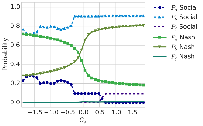
(a)

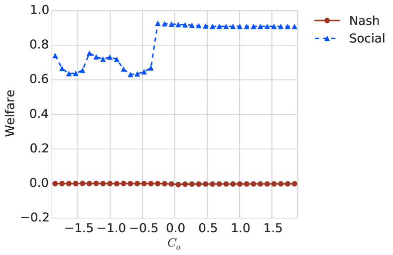
(b)

Figure 1: (a) Nash and socially optimal equilibria for on-street vs. other modes of transit balk, join, observe game. (b) Social welfare and Nash-induced welfare. We vary $C_{o}$ between $-1.85$ and $1.85$ (negative values of $C_{o}$ mean the drivers are incentivized to observe) and all other parameters have the following values: $\lambda=1/5$, $c=30$, $\mu=1/120$, $C_{p}=0.05$, $R=75.0$, $n=100$, $C_{w}=1.5$.

On the other hand, the socially optimal strategy $(P_{o}^{so},P_{b}^{so},P_{j}^{so})\in\Delta_{2}$ is determined by maximizing the social welfare which is given by

$$U_{so}^{n}(P) =\textstyle P_{j}U_{j}^{n}(P)+P_{o}U_{o}^{n}(P)+P_{b}U_{b}^{n}(P)$$ (26)

$$=\textstyle P_{j}\lambda\sum_{k=0}^{n-1}p_{k}^{n}\beta_{k}+P_{o}\lambda\left(\sum_{k=0}^{n_{b}-1}p_{k}^{n}\beta_{k}-C_{o}\right).$$ (27)

As we stated in the previous section, it is well known that, in general, the social welfare is not maximized by the Nash equilibrium and the Nash induced welfare is generally less than the social welfare. For the unobservable queueing game, we compare these the Nash and the social welfare solutions for various parameters combinations including parameters from real-world data obtained from the Seattle Department of Transportation. In Figure 1b, we show an example of how the socially optimal welfare changes as a function of the cost of observing $C_{o}$ while the Nash-induced welfare stays the same roughly the same. However, both the Nash equilibrium and the socially optimal equilibrium vary (Fig. 1a)

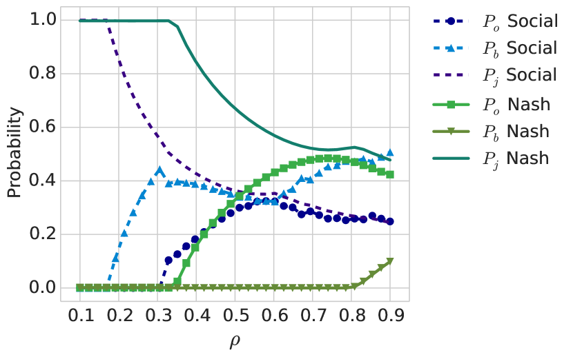
(a)

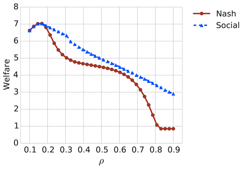
(b)

Figure 2: (a) Nash and socially optimal equilibria. (b) Nash induced welfare vs. maximum social welfare (under socially optimal strategy). For both plots, the game we consider is on-street parking vs. off-street parking and we varied $\rho=\frac{\lambda}{c\mu}$ by keeping $\mu=1/120$ and $c=30$ constant and allowing $\lambda\in[0.025,0.225]$. The other parameter values are $C_{p}=0.05$, $C_{o}=3.85$, $R=95$, $C_{w}=1.5$, $n=100$, $C_{off}=0.962$.

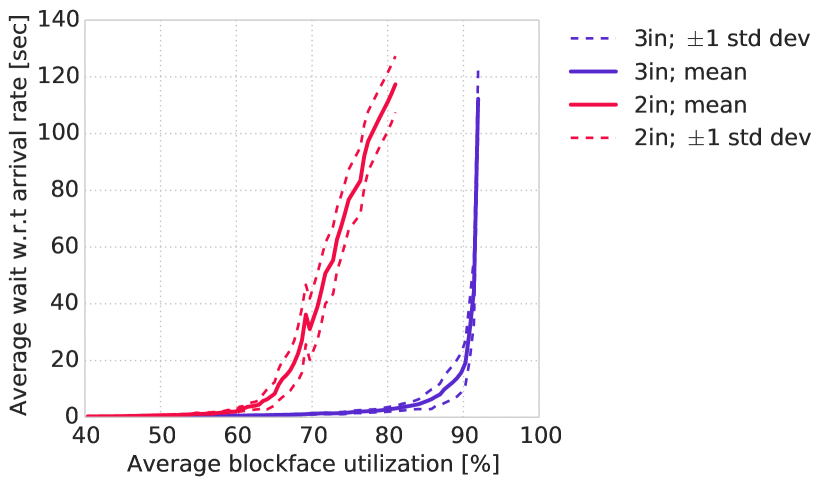
Figure 3: Average wait time (proxy for congestion) with respect to the exogenous arrival rate $\lambda\in[0.6,1.3]$ and fixed service rate per blockface $(c*\mu=1.0)$ plotted against the average block face utilization (proxy for occupancy) for a three node queue–flow network with arrivals injected at all three nodes (green) and only at two nodes (blue). There is a distinct difference in the occupancy vs. congestion curves depending on the network structure and average waits grow unboundedly as $\rho\rightarrow 1$.

IV-A Example: On-Street vs. Off-Street Parking

We now consider that the balking option is to select off-street parking as we did in Section III-B. In particular, we define $U_{b}^{n}=U_{off}=R-C_{off}/\mu$. The Nash equilibrium can be computed using Algorithm 1 using $U_{b}^{n}=U_{off}=R-C_{off}/\mu$ instead of $U_{b}^{n}=0$. On the other hand, the social welfare is now given by

$$U_{so}^{n}(P) =P_{j}U_{j}^{n}(P)+P_{o}U_{o}^{n}(P)+P_{b}U_{b}^{n}(P)$$ (28)

$$\textstyle=P_{j}\lambda\sum_{k=0}^{n-1}p_{k}^{n}\beta_{k}+P_{o}\lambda\left(\sum_{k=0}^{n_{b}-1}p_{k}^{n}\beta_{k}-C_{o}\right)$$

$$\textstyle\qquad+P_{b}\lambda\left(R-\frac{C_{off}}{\mu}\right).$$ (29)

In Figure 2, we show the Nash equilibrium and the socially optimal strategy as well as the welfare as a function of $C_{o}$ for both cases for an example on-street vs. off-street game.

V Queue–Flow Network Simulations

In this section, we present a queue-flow network model over which the games of the previous two sections are impose. Further, we show the results of simulating queue-flow networks with different parameters.

V-A Queue-Flow Simulator

Our simulator is written in Python and is freely available to download and test. Requirements and basic instructions are available on Github. The simulator constructs a syncrhonized list of blockface (drivers in service) and street (drivers waiting/circling) timers linked according to the street topology. For simplicity the simulator treats streets and blockfaces independently: once a driver reaches the end of their drive time on a street, they immediately check the entire blockface they’ve arrived at for availability. If no parking is available, the driver chooses a new destination uniformly at random based on the blockfaces currently accessible to them according to the street topology. High timer resolution is maintained to diminish the likelihood of events occurring simultaneously and curbing potential arguments over available parking (e.g. a driver circling the block arriving at the same blockface as a new, exogenous arrival from outside the system).

In our current experimental setup, drive times between blockfaces are fixed, but could potentially be congestion limited, where drive time would be a function of the number of cars driving on a street between blockfaces. We consider a 3 block face system with 10 parking spaces each, completely connected by two-way streets. Although each blockface can be considered to have its own exogenous arrival rate, to facilitate the game strategies, we have a single source with arrival rate $\lambda$. Drivers who do not immediately choose to balk arrive at a uniformly random blockface where they either observe or join directly.

V-B Congestion vs. Occupancy

The congestion–occupancy relationship is an important one to understand when it comes to designing the price of parking or information—e.g. using a smart device with a subscription fee to observe congestion in various parking zones—in order to reduce parking-related congestion. Many municipalities and researchers design pricing schemes to target a single occupancy level—typically %80—for all blockfaces in a city. Not taking into account the network topology and node type—source or sink—can be detrimental to a pricing scheme. In Figure 3, using the queue–flow simulator for a queue–flow network with three queues, we show that the congestion–occupancy relationship can be drastically different depending on how many nodes are treated as sources for injections. In particular, the upper bound for utilization (before wait time exponentially increases) for the 3-node injection case is around 88% while the 2-node injection case is around 65%. The queue–flow modeling paradigm alone can be a useful tool for designing discriminative pricing or information schemes, accounting for network topology.

On-Street Parking vs. Other Modes of Transit		Equilibrium
Parameters	Type	$(P_{o},P_{b},P_{j})$	Utilization	Avg. Wait	Welfare
$\lambda=1/5$, $C_{o}=0.25$, $R=75$, $C_{w}=0.8$, $C_{p}=0.05$	SO	$(0.00,0.58,0.42)$	$33.2$%	$0.002$	$2.80$
	N	$(0.85,0.13,0.02)$	$69.3$%	$0.359$	$0.00$
$\lambda=1/4.85$, $C_{o}=0.5$, $R=75$, $C_{w}=0.75$, $C_{p}=0.05$	SO	$(0.00,0.56,0.44)$	$34.9$%	$0.002$	$3.02$
	N	$(0.84,0.09,0.07)$	$77.9$%	$0.901$	$0.00$
$\lambda=1/4.5$, $C_{o}=2.0$, $R=75$, $C_{w}=0.5$, $C_{p}=0.075$	SO	$(0.00,0.4,0.6)$	$52.3$%	$0.04$	$4.27$
	N	$(0.55,0.00,0.45)$	$88.0$%	$3.69$	$2.68$
On-Street vs. Off-Street Parking
Parameters	Type	Eq.: $(P_{o},P_{b},P_{j})$	Utilization	Avg. Wait	Welfare
$\lambda=1/4.5$, $C_{o}=3.85$, $R=65$, $C_{w}=1.5$, $C_{off}=0.962$,	SO	$(0.47,0.19,0.34)$	$69.9$%	$1.99$	$6.58$
$C_{p}=0.05$	N	$(0.49,0.00,0.51)$	$84.0$%	$7.77$	$1.85$
$\lambda=1/4.75$, $C_{o}=3.85$, $R=65$, $C_{w}=1.5$, $C_{off}=0.962$,	SO	$(0.5,0.14,0.36)$	$70.6$%	$2.23$	$9.23$
$C_{p}=0.05$	N	$(0.53,0.00,0.47)$	$81.0$%	$5.96$	$7.19$

TABLE I: Queue–Flow Network Game Simulation Results: for each of the simulations we set the total number of parking spaces to be $c=30$, the average parking duration is $120$ minutes ($\mu=1/120$) which is consistent with the Seattle Department of Transportation data. We use the shorthand SO for socially optimal and N for Nash.

V-C Costly Observation Queuing Game Simulations

Coupling the queue-flow network with the game theoretic models of the previous sections, we simulate the queueing game and its impact on network flow (average wait time) and on-street parking utilization (occupancy). Given a queue-flow network topology, for simplicity, we assume that each of the queues has the same service rate $\mu$. In addition, we suppose that the total number of parking spots (servers) across all queues in the network is $c$, the arrival rate to the queuing network is $\lambda$, and the capacity of queue-flow network is $n$. This allows us to model the whole queuing system as a M/M/$c$/$n$ queue to which we apply the costly observation queuing game for various parameters combinations.

We execute our simulation as follows. First, we determine the equilibrium of the game—or the socially optimal strategy depending on which we intend to simulate—and then, we use the simulator described above to determine the average waiting time and utilization. The game only effects the arrival process of the queue–flow network; once arriving drivers enter the network, the queue–flow simulator determines the drivers impact on the system and the waiting time they experience.

Given a strategy $(P_{o},P_{b},P_{j})$—either a Nash equilibrium computed via Algorithm 1 or a social optimum computed by maximizing (27)—we sample from the Poisson distribution with parameter $1/\lambda$ to determine the arrival time of the next driver. Then, we sample from the distribution determined by $(P_{o},P_{b},P_{j})$ to decide if the arriving driver will balk, join without observing, or pay to observe. If the driver balks, then we discard this arriving car. If the driver joins without observing, then we determine which node the driver enters by randomly choosing (using a uniform distribution) a queue in the network. If the driver pays to observe, then we examine the length of each queue in the system and the driver joins the queue with the shortest length as long as it is less than the balking rate.

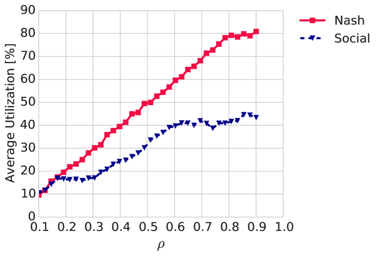
(a)

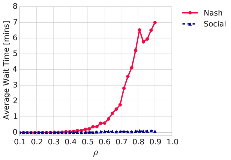
(b)

Figure 4: (a) Average wait time (a) and (b) average blockface utilization as a function of $\rho=\frac{\lambda}{c\mu}$ where $c=30$ and $\mu=1/120$ are fixed and $\lambda\in[0.025,0.225]$ for a three node system. The other parameter values are $C_{p}=0.05$, $C_{o}=3.85$, $R=95$, $C_{w}=1.5$, $n=100$, $C_{off}=0.962$. The Nash equilibrium and the socially optimal equilibrium varies with $\rho$ and is depicted in Figure 2.

In Table I, we show the results of simulations for both the costly observation game simulations for the costly observation queuing game and the on-street vs. off-street example. We explore different parameter combinations and show the utilization rate, average wait time, social welfare, and the Nash-induced welfare. The social welfare is always higher than the Nash welfare, which is to be expected. The utilization rate and average wait time are always less under the socially optimal strategy than the Nash equilibrium.

In Figure 4, we show the result of simulating both the Nash equilibrium and the socially optimal strategy for various values of the traffic intensity $\rho$ (holding all other parameters fixed). These simulations are for the same games depicted in Figure 2. As the traffic intensity increases, we see that both the Nash and socially optimal utilization increase almost linearly with the Nash utilization remaining greater. The socially optimal equilibrium in all cases keeps waiting times for parking—our current surrogate for congestion—uniformly less than the Nash equilibrium. Intuitively this makes sense: given a finite resource—parking—the socially optimal strategy ensures this resource is more freely available. On the other hand, the Nash strategy more efficiently utilizes the resource to the extent of its availability. Another interesting thing to notice is the drop in wait time for the Nash solution at $\rho=0.8$. If we look at Figure 2b, we see that the probability for balking $P_{b}$ in the Nash solution suddenly becomes non-zero at $\rho=0.8$. This is likely to be the cause of the drop in wait time; however, as $\rho\rightarrow 1$, we expect the wait time to blow-up so that after the drop, wait time continues to increase.

Of the two scenarios (costly observation and on-street vs. off-street), the on-street vs. off-street parking more closely resembles reality in the sense that the off-street option exists. One might guess then, that a user will maximize their utility in either the Nash or socially optimal case by frequently taking advantage of the ability to observe before choosing where to park, given the nature and travel constraints of the system. What surprises us is that only partial information availability amongst the users—as seen in Table I, Figures 1 and 2 where $P_{o}\neq 1$ for the socially optimal solution—is required to increase social welfare. Moreover, it seems the socially optimal equilibrium strategy requires less information availability.

From a municipality’s perspective, this is a useful result when designing a socially optimal parking infrastructure. Not everyone will know information about parking availability in the first place (e.g. tourists vs. residents). Even from a more practical point of view, this is a useful result in that reaching 100% information availability for all drivers is an economically infeasible task, requiring more resources than could likely be justified.

VI Discussion and Future Work

We presented a framework for modeling parking in urban environments as parallel queues and we overlaid a game theoretic structure on the queuing system. We investigated both the case where drivers have full information—i.e. observe the queue length—and where drivers have to pay to access this information. We show in both cases that the social welfare is less under the Nash equilibrium than the socially optimal solution and we show that only partial information is required to increase social welfare. Finally, through simulations we connect the queuing game to a flow network model in order to characterize wait time (congestion) versus utilization (occupancy).

In future work, by capitalizing on the game-theoretic model, we aim to use a mechanism design framework to shift the user-selected equilibrium to a more socially efficient one by selecting the cost of information and the price of parking that optimizes social welfare. Furthermore, we plan to optimize the for the amount parking-related congestion that contributes to over all congestion; in particular, we plan to optimize the social welfare as a function of the capacity of the queue. We plan to relax the homogeniety assumption by considering players with different preferences such as walking time to destination and different priority levels such as disabled placard holders. Furthermore, we aim to couple the parallel queue game model with classical network flow models for traffic flow so that we can develop an understanding of the fundamental relationship between congestion and parking. We view the work in this paper as the first steps toward developing a comprehensive modeling paradigm in which the queuing behavior for parking and traffic flow are captured.

References

- [1] H. Frumkin, “Urban sprawl and public health,” Center for Disease Control, Tech. Rep. 17, May–June 2002.
- [2] D. B. Resnik, “Urban sprawl, smart growth, and deliberative democracy,” Amer. J. Public Health, vol. 100, no. 10, pp. 1852–1856, 2010.
- [3] D. Schrank, B. Eisele, T. Lomax, and J. Bak, “2015 urban mobility scorecard,” Texas A&M Transportation Institute and INRIX, Tech. Rep., 2015.
- [4] J. I. Levy, J. J. Buonocore, and K. von Stackelberg, “Evaluation of the public health impacts of traffic congestion: a health risk assessment,” Environ Health, vol. 9, no. 1, p. 65, 2010.
- [5] K. Zhang and S. Batterman, “Air pollution and health risks due to vehicle traffic,” Science of The Total Environment, vol. 450–451, pp. 307–316, Apr 2013.
- [6] D. Shoup, “Cruising for parking,” Transport Policy, vol. 13, pp. 479–486, 2006.
- [7] D. C. Shoup, “Truth in Transportation Planning,” Transporation and Statistics, vol. 6, no. 1, 2003.
- [8] F. Caicedo, C. Blazquez, and P. Miranda, “Prediction of parking space availability in real time,” Expert Systems with Applications, vol. 39, no. 8, pp. 7281 – 7290, 2012.
- [9] K. Chen, J. jun Wang, and F. Han, “The research of parking demand forecast model based on regional development,” in Proc. 12th COTA Inter. Conf. of Transportation Professionals, 2012, pp. 23–29.
- [10] K. Sasanuma, “Policies for parkingpricing derived from a queueing perspective,” Master’s thesis, MIT, 2009.
- [11] C. Tiexin, T. Miaomiao, and M. Ze, “The model of parking demand forecast for the urban CCD,” Energy Procedia, vol. 16, Part B, pp. 1393 – 1400, 2012.
- [12] P. Bolton and M. Dewatripont, Contract Theory. MIT Press, 2005.
- [13] San Francisco parking pilot evaluation, SFpark, conducted by San Francisco Municipal Transportation Authority, [Online:] http://sfpark.org/.
- [14] G. Pierce and D. Shoup, “Getting the prices right,” J. American Planning Association, vol. 79, no. 1, pp. 67–81, 2013.
- [15] J. Glasnapp, H. Du, C. Dance, S. Clinchant, A. Pudlin, D. Mitchell, and O. Zoeter, “Understanding dynamic pricing for parking in los angeles: Survey and ethnographic results,” HCI in Business, pp. 316–327, 2014.
- [16] N. Carney. (2013) Bringing markets to meters. [Online]. Available: http://datasmart.ash.harvard.edu/news/article/bringing-markets-to-meters-312
- [17] D. Gross, Fundamentals of queueing theory. John Wiley & Sons, 2008.
- [18] J. Walrand, “A probabilistic look at networks of quasi-reversible queues,” IEEE transactions on information theory, vol. 29, no. 6, pp. 825–831, 1983.
- [19] N. Knudsen, “Individual and social optimization in a multiserver queue with a general cost-benefit structure,” Econometrica, vol. 40, no. 3, pp. 515–528, 1972.
- [20] R. Hassin and R. Roet-green, “Equilibrium in a two dimensional queueing game: When inspecting the queue is costly,” Working Paper, December 2011. [Online]. Available: http://www.math.tau.ac.il/~hassin/ricky.pdf
- [21] J. Nash, “Non-cooperative games,” Annals of Mathematics, vol. 54, no. 2, pp. 286–295, 1951.