Flavor-changing decays of the top quark in 5D Warped Models

Abstract

We study flavor changing neutral current decays of the top quark in the context of general warped extra dimensions, where the five dimensional metric is slightly modified from 5D anti-de-Sitter (AdS₅). These models address the Planck-electroweak hierarchies of the Standard Model and can obey all the low energy flavor bounds and electroweak precision tests, while allowing the scale of new physics to be at the TeV level, and thus within the reach of the LHC at Run II. We perform the calculation of these exotic top decay rates for the case of a bulk Higgs, and thus include in particular the effect of the additional Kaluza-Klein (KK) Higgs modes running in the loops, along with the usual KK fermions and KK gluons.

I Introduction

Extra-dimensional models with warped space-time geometry provide a simple and elegant way to understand the hierarchy problem. In the original models (Randall Sundrum, or RS Randall:1999vf ), the Standard Model (SM) is embedded in a slice of anti de Sitter space (AdS₅) with two manifolds bounding the extra dimension: one at the Planck scale, the other at the TeV scale. Warping induces an exponential hierarchy between the effective cutoff scales of the theory at the two manifolds. The smallness of the electroweak symmetry breaking (EWSB) scale emerges due to a low cutoff near the TeV brane, while the high scale of gravity is generated at the other end. If all the SM fields live on the TeV brane, the model cannot solve the SM flavor puzzle, and higher dimensional operators induce large flavor-changing neutral currents (FCNC) disallowed by the low energy data. Allowing the SM fermion fields to leak into the bulk bulk can help resolving the flavor hierarchy problem, but is not always sufficient to protect RS from severe flavor and electroweak constraints constraints . The reason is that in these models, the interactions of ordinary quarks with the KK gauge bosons are non-universal in flavor, which induces tree level FCNC processes mediated by these heavy gauge bosons. Constraints from the CP violating observable in the kaon system, $\epsilon_{K}$, result in generic bounds on the mass of the lightest KK gauge boson excitation (KK gluon) of 10-20 TeV. Moreover, because of the mixing of the KK gauge bosons with the SM $Z$ boson within EWSB, the $Z$ couplings to quarks become flavor non-universal, producing dangerous contributions to electroweak precision observables. With such heavy KK masses, there is hardly any hope of seeing such models at the LHC at the present run lhc .

There are different resolutions available in the literature to deal with these constraints. One is to enlarge the gauge field to $SU(3)_{c}\times SU(2)_{L}\times SU(2)_{R}\times U(1)_{X}\times P_{LR}$, where the additional symmetries of $SU(2)_{R}$ and $P_{LR}$ to the $T$ parameter offer custodial protection to $Zq_{L}^{i}{\bar{q}}_{L}^{j}$ vertices and lower the constraints on the KK scales to 2-3 TeV Agashe:2003zs . Another possibility is to include brane kinetic terms for gauge and fermion fields propagating in the bulk, yielding first KK mode masses of the order of a few TeV Carena:2004zn , with precision bounds under control. Another alternative is to introduce a dilatonic scalar to allow for a deformation of the space-time metric such that it deviates from the AdS₅ structure in the infrared region (near the TeV brane), while it approaches AdS₅ asymptotically in the UV brane Falkowski:2008fz ; Batell:2008me ; Cabrer:2011fb ; Carmona:2011ib . In the particular model studied in Cabrer:2011fb , the IR brane is close to a naked metric singularity, outside the physical interval. The proximity of the singularity provides a strong wave-function renormalization for the Higgs field, which suppresses additional contributions to the $T$ and $S$ parameters, and can render the theory valid for KK masses $M_{KK}\sim$ 1-3 TeV.

With Run II at the LHC, we are entering the precision era for the SM Higgs physics, but the LHC is also known for being an effective top quark factory, with millions of top quarks being produced yearly, and cross sections for pair productions reaching 1 $nb$. The experimental achievements have induced a concerted effort to improve the theoretical estimates. Deviations from SM, either in direct particle production or indirectly through higher order effects, and/or observables suppressed in the SM constitute areas of useful examination. Loop-induced dipole operators in warped space models exhibit a non-trivial dependence on the Higgs profile, such that the contribution is saturated as the Higgs approaches the IR brane, and decreases when the Higgs field is leaking out towards the UV brane Delaunay:2012cz . Recently, it has been shown that by including KK excitations of the SM Higgs boson in loop diagrams (in particular, in those yielding dipole operators of SM fermions), the effect of summing over enough KK modes in the brane limit can add up and increment the value of the amplitudes by some order 1 factors Agashe:2014jca .

FCNC processes of the top quark are extremely suppressed in the SM, and in supersymmetry an enhancement is expected in $b\to s\gamma$ rather than $t\to c\gamma$ Cao:2007dk , due to allowed values of $\tan\beta$. In the SM, ${\cal B}(t\to qX)\simeq 10^{-17}-10^{-12}$, for $q=c,u$ and $X=Z,g,\gamma,H$ AguilarSaavedra:2004wm . Thus these decays are suppressed in the SM and indicate that any significant enhancements could signal New Physics effects.

Models have been designed where ${\cal B}(t\to c\gamma)$ can reach $10^{-12}-10^{-7}$. In models with extra quarks, ${\cal B}(t\to qZ)\simeq 1.1\times 10^{-4}$, ${\cal B}(t\to qH)\simeq 4.1\times 10^{-5}$, and ${\cal B}(t\to q\gamma)\simeq 7.5\times 10^{-9}$, ${\cal B}(t\to qg)\simeq 1.5\times 10^{-7}$ AguilarSaavedra:2002kr . In Two-Higgs Doublet Models which violate FCNC at tree level, ${\cal B}(t\to cH)\simeq 1.5\times 10^{-3}$, ${\cal B}(t\to uH)\simeq 5.5\times 10^{-6}$, and the radiative decays ${\cal B}(t\to cZ)\simeq 10^{-7}$, ${\cal B}(t\to c\gamma)\simeq 10^{-6}$ and ${\cal B}(t\to cg)\simeq 10^{-4}$ Atwood:1996vj . In Two-Higgs doublet models ${\cal B}(t\to cZ)\simeq\times 10^{-10}$, ${\cal B}(t\to c\gamma)\simeq\times 10^{-9}$, ${\cal B}(t\to cg)\simeq 10^{-8}$ and ${\cal B}(t\to cH)\simeq 10^{-5}$ Luke:1993cy . In MSSM, the largest results are obtained assuming non-universal squark masses, and these are ${\cal B}(t\to qZ)\simeq 2\times 10^{-6}$, ${\cal B}(t\to q\gamma)\simeq 2\times 10^{-6}$, ${\cal B}(t\to qg)\simeq 10^{-4}$ and ${\cal B}(t\to qH)\simeq 10^{-5}$ Cao:2007dk . The decay $t\to c\gamma$ was also evaluated in top color assisted technicolor model Cao:2007bx , little Higgs models Han:2009zm , models with universal extra dimensions GonzalezSprinberg:2007zz and within the context of effective theories Aranda:2009cd . The dipole operators have been explored before in warped extra dimensions Csaki:2010aj , and the decay $t\to c\gamma$ was investigated in the context of warped extra dimensional models in Gao:2013fxa , for brane-localized Higgs in models with custodial symmetry.

The best experimental limits come from searches of FCNC decays at the LHC. ATLAS Aad:2015uza has published a compilation of limits based on the full 8 TeV data set at 20.3 $fb^{-1}$. The bounds are: ${\cal B}(t\to qZ)<\times 0.07(0.08)$ %, ${\cal B}(t\to u\gamma)<0.0161(0.0279)$ %, ${\cal B}(t\to c\gamma)<0.182(0.261)$ % for the observed(expected) limits. In addition, results from both ATLAS Aad:2015uza and CMS CMS003 perform the search in single top production for the decay $t\to cg$. The most stringent results come from ATLAS, yielding ${\cal B}(t\to qg)<4.0\times 10^{-5}$ and ${\cal B}(t\to c\gamma)<1.7\times 10^{-4}$ Aad:2015uza . A review of current experimental constraints and theoretical predictions is presented in Agashe:2013hma .

In this work we investigate the contribution to the FCNC top quark decay in a general warped scenario, which allows a slight modification of the warping factor along the extra dimension, allowing it to deviate slightly from the AdS₅ metric Cabrer:2011fb . This deviation is such that the warping is more drastic near the TeV brane, while the background becomes more AdS₅-like near the Planck brane. These models suppress additional contributions to electroweak precision variables in the same parameter space region where contributions to Higgs production cross section Frank:2013qma and decay rates Frank:2015zwd are consistent with experimental bounds, and this is achievable only for bulk Higgs. We perform the calculation including fermion profiles consistent with the SM masses and the CKM quark mixing matrix, and sum over all the fermion and Higgs boson KK modes in the loops up to the third KK states. We are particularly interested in the role of the KK excitations of the Higgs boson.

Our work is organized as follows. In Sec. II we introduce briefly the general warped space model, with emphasis on the Higgs and fermion zero-mode and KK states. In Sec. III.1 we analyze the tree-level decays, while in Sec. III.2 present the results for the FCNC dipole decay of the top quark. We conclude in Sec. IV and leave some of our analytic expressions for the Appendix (V).

II Warped Space Models with fields in the bulk

Consider the SM fields propagating in a 5D space with an arbitrary metric $A(y)$ such that the metric is:

$$ds^{2}=e^{-2A(y)}\eta_{\mu\nu}dx_{\mu}dx_{\nu}+dy^{2}$$

where $\eta_{\mu\nu}=diag(-1,1,1,1)$. This is the most general ansatz consistent with Minkowski spacetime in 4D. A naked singularity is located at $y=y_{s}$ such that the IR brane is located a short distance from that singularity, at $y=y_{1}=y_{s}-\Delta$, by means of a stabilizing dilatonic field:

$$\Phi(y)=-\frac{\sqrt{6}}{\nu}\log\left[\nu^{2}k(y_{s}-y)\right],$$ (1)

with $k$ the inverse curvature radius of the AdS₅ space-time and $\nu$ a real parameter, corresponding to the metric:

$$A(y)=ky-\frac{1}{\nu^{2}}\log\left(1-\frac{y}{y_{s}}\right).$$ (2)

The modified AdS₅ metric mimics that of the RS models $A(y)=ky$, for $y\to 0$, while drastically departing from it for $y\to y_{s}$. In this model, the hierarchy problem is solved by assuming a Higgs potential of the form

$$V(H)=k^{2}\left[a(a-4)-4ae^{\nu\Phi/\sqrt{6}}\right]|H|^{2}$$ (3)

We define the CP-even Higgs field as

$$H(x,y)=\frac{1}{\sqrt{2}}\left(\begin{array}[]{c}0\\ h(y)+\xi(x,y)\end{array}\right)$$ (6)

where $h(y)$ is the Higgs background vacuum expectation value (VEV) profile determined by the equations of motion and boundary conditions given by

$$h(y)=h_{0}e^{aky}\bigg{[}1+(M_{0}/k-a)\left[F(y)-F(0)\right]\bigg{]}\,,$$ (7)

where $h_{0}$ is a normalization factor and $M_{0}$ is the brane Higgs mass term (the coefficient of the Higgs boundary potential $|H|^{2}\delta(y-y_{1})$ at the IR brane) introduced to give rise to the Higgs zero mode with the correct physical mass. The function $F(y)$ given by

$$F(y)=e^{-2(a-2)ky_{s}}ky_{s}\left[-2(a-2)ky_{s}\right]^{-1+4/\nu^{2}}\Gamma\left[1-\frac{4}{\nu^{2}},-2(a-2)k(y_{s}-y)\right],$$ (8)

is a generalization of the corresponding RS function $F(y)=e^{-2(a-2)ky}$. Here $a$ is the parameter that determines the localization of the Higgs field. The large $a$ limit ($a\gg 2$) corresponds to a brane-localized Higgs, while for $a$ of order $1$ we say that the Higgs is a bulk Higgs field. Note that there is a minimum value of $a$ that ensures that no new fine-tuning is introduced in the model in order to solve the hierarchy problem; $a_{min}=2$ for RS models, $a_{min}>2$ for modified AdS₅ models Cabrer:2011fb ; Frank:2013un ; Frank:2013qma ; Frank:2015zwd .

In general, the oblique precision electroweak parameter $T$ is enhanced by the compactification volume $ky_{1}$ and it is the most constraining of the oblique parameters, while $S$ does not depend on the volume. In RS, compatibility with electroweak precision data imposes a lower bound of around $M_{KK}\mathrel{\raise 1.29167pt\hbox{$>$\kern-7.5pt\lower 4.30554pt\hbox{$\sim$}}}13$ TeV at the 95% CL constraints , bound which can improve when the Higgs is delocalized from the IR brane Agashe:2008uz . For $a\geq 2$, the $M_{KK}$ scale bound becomes $M_{KK}\mathrel{\raise 1.29167pt\hbox{$>$\kern-7.5pt\lower 4.30554pt\hbox{$\sim$}}}7$ TeV at the 95% CL. In modified AdS₅ models, the different behavior of the Higgs profile at the IR brane location $y_{1}$ results in much more relaxed bounds on the KK scale. As KK modes are localized towards the IR brane, their overlapping integrals with the Higgs (and therefore their contribution to the electroweak parameters $T$ and $S$) depend on the values of the physical Higgs wave functions at the IR brane. The scale of new physics $M_{KK}$ could be as low as 0.8 TeV Cabrer:2011fb , for the Higgs and metric parameters $a=3.1$ and $\nu=0.5$, while for $\nu\mathrel{\raise 1.29167pt\hbox{$>$\kern-7.5pt\lower 4.30554pt\hbox{$\sim$}}}5$ one starts to recover the RS results.

These models have also been tested by comparing their predictions for Higgs boson production for bulk Higgs, in the original RS metric and within a modified metric background Frank:2013un ; Frank:2013qma ; Frank:2015zwd . In 5D scenarios with modified AdS₅ metric, the results are consistent with the LHC Higgs measurements in the same region of the parameter space where flavor and precision electroweak constraints are satisfied. Thus a safe region of parameter space (minimum UV sensitivity and safe from non-perturbative couplings) exists, requiring moderate 5D Yukawa couplings $Y^{5D}\sim 1$, as well as low Higgs localization parameter values, $a\sim 2-5$.

For fermions, using values for $Y_{5D}\sim 1$ and localizations coefficients $c$, for the zero mode profiles for which full analytical expressions are available Frank:2013un , we construct the Yukawa coupling matrix and the mass matrix with the following elements

$$(y^{0}_{u})_{ij}=\frac{(Y^{5D}_{u})_{ij}}{\sqrt{k}}\int_{0}^{y_{1}}dye^{-4A(y)}h(y)q^{0,i}_{L}(y)u^{0,j}_{R}(y)\,,$$ (9)

where $Y_{u}^{5D}$ are the 5D dimensionless Yukawa couplings, $u$ stands for up and down $SU(2)$ singlet quarks, and $q^{0,i}_{L}(y)$ represent zero mode SM doublets. One can then construct the KK profiles for fermions through solving the differential equations numerically for all the 6 flavors of the fermion profiles:

$$\partial_{y}\left(e^{(2c-1)A(y)}\partial_{y}\left(e^{-(c+2)A(y)}\right)\right)f(y)+e^{(c-1)A(y)}m_{n}^{2}f(y)=0$$ (10)

imposing Dirichlet boundary conditions for the “wrong” chirality fermions. The overlap integrals along the extra dimension lead to the effective 4D Yukawa coupling matrix, which in the up sector can be writen as

$${\bf Y}_{u}=\left(\begin{array}[]{ccc}(y^{0}_{u})_{3\times 3}&(0)_{3\times 3N}&(Y^{qU})_{3\times 3N}\\ (Y^{Qu})_{3N\times 3}&(0)_{3N\times 3N}&(Y_{1})_{3N\times 3N}\\ (0)_{3N\times 3}&(Y_{2})_{3N\times 3N}&(0)_{3N\times 3N}\end{array}\right),$$ (11)

with the down sector Yukawa matrix ${\bf Y}_{d}$ computed in the same way. The submatrices are obtained by the overlap integrals

$$Y^{qU}=\frac{(Y^{5D}_{u})_{ij}}{\sqrt{k}}\int_{0}^{y_{1}}dye^{-4A(y)}h(y)q^{0,i}_{L}(y)U^{n,j}_{R}(y)$$ (12)

$$Y^{Qu}=\frac{(Y^{5D}_{u})_{ij}}{\sqrt{k}}\int_{0}^{y_{1}}dye^{-4A(y)}h(y)Q^{m,i}_{L}(y)u^{0,j}_{R}(y)$$ (13)

$$Y_{1}=\frac{(Y^{5D}_{u})_{ij}}{\sqrt{k}}\int_{0}^{y_{1}}dye^{-4A(y)}h(y)Q^{m,i}_{L}(y)U^{n,j}_{R}(y)$$ (14)

$$Y_{2}=\frac{(Y^{5D^{*}}_{u})_{ij}}{\sqrt{k}}\int_{0}^{y_{1}}dye^{-4A(y)}h(y)Q^{m,i}_{R}(y)U^{n,j}_{L}(y)\,,$$ (15)

where the indices $m$ and $n$ track the KK level and $i,j=1,2,3$ are 5D flavor indices. We have included 3 full KK levels so that the Yukawa matrices in the gauge basis are $21\times 21$ dimensional matrices.

The 4D effective $21\times 21$ fermion mass matrix (constructed in a similar way) is not diagonal due to electroweak symmetry breaking, and must be diagonalized in order to go to the physical mass basis. Once in that basis, we obtain the physical Yukawa couplings by appropriately rotating the Yukawa matrix in Eq. (11). As pointed out before, the Yukawa couplings in the mass basis can receive important corrections in these scenarios Azatov:2009na ; Frank:2015sua ; Frank:2013un . Quite plausibly, these effects could add-up and maybe enhance further loop-dominated flavor violating (FV) decays of the top quark, where, similar to Higgs production and decay processes, all KK excitations (for Higgs and fermions) will contribute. We investigate this in the following section.

III Phenomenology of FCNC decays of the top quark

For the phenomenology section of this work we have considered the parameter region of the modified $AdS_{5}$ model with $\nu\simeq 0.5$ and $kL(y_{1})\simeq 0.2$, which is the curvature of space at the location of the IR brane given by

$$kL(y_{1})={k\Delta_{1}\nu^{2}\over\sqrt{1-2\nu^{2}/5+2k\Delta_{1}\nu^{2}+(k\Delta_{1})^{2}\nu^{4}}},$$ (16)

with $\Delta_{1}$ being the distance between the position of the curvature singularity and the IR brane, $\Delta_{1}\equiv y_{s}-y_{1}$. This region of parameter space allows for the lowest possible KK scales of about $700$ GeV, which are still consistent with the electroweak precision test parameter bounds Cabrer:2011fb . We have considered scenarios with 5 different KK gluon mass scales at about $\sim 700$ GeV, $1000$ GeV, $1300$ GeV, $1700$ GeV and $2300$ GeV. (Note that constraints from flavor processes might still force the KK scale to be 1-2 TeV Cabrer:2011fb ). These masses are achieved through slightly changing the length of the extra dimension by fixing $A(y_{1})$ around $\simeq 36-37$. Once the KK scale has been fixed, we calculate the minimum $a$-parameter (corresponding to the maximally delocalized Higgs field along the 5th dimension) that satisfies the constraint $|F(y_{1})|\equiv\delta=1$, where $F(y)$ is given by Eq. (8). This constraint ensures that the Higgs profile solution which leaks towards the UV brane is still IR dominated, without requiring a fine tuning of parameters ($M_{0}/k-a=0$). We have considered 4 values of the $a$-parameter for each of the KK mass scales mentioned above, all corresponding to a heavily delocalized bulk Higgs field with $a\in\{a_{min},a_{min}+0.5,a_{min}+1,a_{min}+1.5\}$, very close to the values $a\simeq 3$, $3.5$, $4$ and $4.5$.

Having calculated the lowest $a$-parameter of each model, we scan the parameter space of the 5D-fermion $c$-parameters and the 5D Yukawa couplings, $Y^{5D}$. The $c$-parameters correspond to the bulk mass parameter of fermions (localization of fermions along the 5th dimension) and we need to find a set of these parameters, $\{c_{q_{i}},c_{u_{i}},c_{d_{i}}\}$, for all of the quark sector fermions ($c_{q}$ corresponds to the $SU(2)$ doublets, $c_{u}$ corresponds to the up-like and $c_{d}$ to the down-like singlets) that, combined with our choice of $Y^{5D}$, yield the correct SM quark masses and CKM mixing angles. For our scan, we consider two orders for the $5D$ Yukawa couplings, $Y^{5D}\simeq 1$ and $Y^{5D}\simeq 3.$ Our approach is such that we randomly choose all the Yukawa couplings and allow for random deviations from guided ranges for the $c$-parameters which produce SM-like masses and mixings. (For example, for UV localized fermions we only scan the range between $0.55-0.7$ and disregard possible points outside of this region.) This way we conduct a first estimation of the masses and CKM parameters by only considering the zero mode fermions, calculating the matrix elements given in Eq. (9) and filter the results to include points that reproduce values close to the SM.

Having fixed the parameters $\nu$, $y_{1}$, $c$’s, $Y^{5D}$’s and $a$, we include the KK modes into our previous naive calculation. As mentioned earlier, we have only considered the full first 3 KK levels. For a highly delocalized Higgs field considered here, heavier modes should decouple fast enough so that the results of considering only the first 3 KK modes are in good agreement with those of including the full tower Frank:2013qma . We solve the differential equations of motion along the 5th dimension to find the masses and profiles of the zero modes and of the KK modes for all the quark sector fermions, the gauge bosons, and the Higgs bosons. Using these profiles we compute the $21\times 21$ Yukawa matrices like the one shown in Eq. (11) for the up-type quarks. We then rotate the quark fields to transform to the mass basis by diagonalizing the up and down fermion mass matrices given by ${\bf M}_{u}={\rm VEV}\times{\bf Y}_{u}+M_{KK}$ where $M_{KK}$ is a $21\times 21$ diagonal matrix whose elements are the masses of the KK modes, $M_{KK}=diag\{0,0,0,M^{up}_{Q_{1}},\dots,M^{top}_{Q_{3}},M^{up}_{U_{1}},\dots,M^{top}_{U_{3}}\}$ (and similarly in the down sector).

In the physical mass basis, ${\bf M}_{u}\rightarrow V^{u}_{L}{\bf M}_{u}V^{u}_{R}$, the Yukawa matrix elements given by ${\bf Y}_{u}\rightarrow V^{u}_{L}{\bf Y}_{u}V^{u}_{R}$ are not diagonal, leading to tree-level Higgs mediated FCNCs. To calculate the CKM matrix, we need to perform the same calculations for the down sector as well. The CKM matrix is given by $(V_{CKM})_{ij}=\left(V^{u}_{L}V_{L}^{d\dagger}\right)_{ij}$, where $i,j=1,2,3$, i.e., it is the $3\times 3$ upper-left corner of the $21\times 21$ charged current mixing matrix $V^{u}_{L}V_{L}^{d\dagger}$. At this point, we proceed to the final scan check and compare the masses and mixings obtained from the $21\times 21$ matrices with those of the SM and discard the phenomenologically inconsistent scan points. We generate in this way 40 different (and viable) parameter space points for each value of the Higgs parameter $a$ and each KK mass scale.

III.1 FV decays of top quark at tree level: $t\to qh$ and $t\to qZ$

Using the results of the previous section, we can read off the coupling strengths of the FCNC decays of the top quark at the tree level. For the $t\to ch$ decay, these are given by the entries $Y^{u}_{23}$ and $Y^{u}_{32}$ and by computing the following branching ratio Casagrande:2008hr ; Azatov:2009na

$${\cal B}(t\rightarrow qh)={2(1-r_{Z})^{2}(1+2r_{Z})\over(1-r_{W})^{2}(1+2r_{W})}\left(|(Y^{u}_{L})_{q3}|^{2}+|(Y^{u}_{L})_{3q}|^{2}+{12\sqrt{r_{q}}r_{Z}\over(1-r_{Z})(1+2r_{Z})}\text{Re}\left[(Y^{u}_{L})^{*}_{q3}(Y^{u}_{L})_{3q}\right]\right)$$ (17)

where $r_{i}\equiv(m_{i}/m_{t})^{2}$, $q=2$ for the branching ratio of top to charm, and $q=1$ for top to up.

The results of this calculation are shown in Fig. 1, where four values of $a$ have been used as explained earlier. Since we have also included five different KK masses, we present the results for the same $a$ but different KK mass, slightly shifted in the $a$ scale.

The branching ratio is expected to depend inversely on the KK scale and directly related to the Yukawa couplings, roughly as $\displaystyle{\cal B}(t\rightarrow qh)\sim\frac{Y_{5D}^{4}}{M_{KK}^{4}}\frac{m_{q}}{v}$ Azatov:2009na . We see that the dependance on the KK mass more or less follows that trend, although for larger 5D Yukawa couplings ($Y^{5D}\sim 3$) the dependence seems milder. This large Yukawa case might be on the verge of validity for our perturbative calculations since the full flavor effects accelerate the appearance of strong coupling effects. Note also that in the case ($Y^{5D}\sim 1$), all Yukawa couplings are order $\sim 1$ (i.e. safer), except for the (33) entry which must still be of order $\sim 3$ in order to generate the top quark mass. This means that even in the smaller Yukawa case there is a somewhat larger flavor effect. Nevertheless no cumulative flavor family enhancements are present in this case, making it safe in terms of perturbativity.

Notice also that as the Higgs becomes more and more localized towards the IR brane, i.e.,  larger values of $a$, the branching ratio increases. This is due to an enhancement of the overlap integrals as the more IR localized Higgs field couples more strongly with the fermion fields . Unfortunately, larger Higgs couplings also lead to stronger bounds from precision electroweak constraints as well as from the Higgs production and decay phenomenology. The threshold is not clear cut, but for the larger values of $a$ considered, one should expect that only the larger KK scales might be safe from constraints. Thus the expected size of the branching ratio for the $t\to ch$ decays should be somewhere around ($10^{-5}$ - $10^{-7}$), and for $t\to uh$ somewhere around ($10^{-6}$ - $10^{-8}$). These last two ranges are consistent with expectations as one would expect a relative strength governed by (very roughly) $m_{u}/m_{c}$.

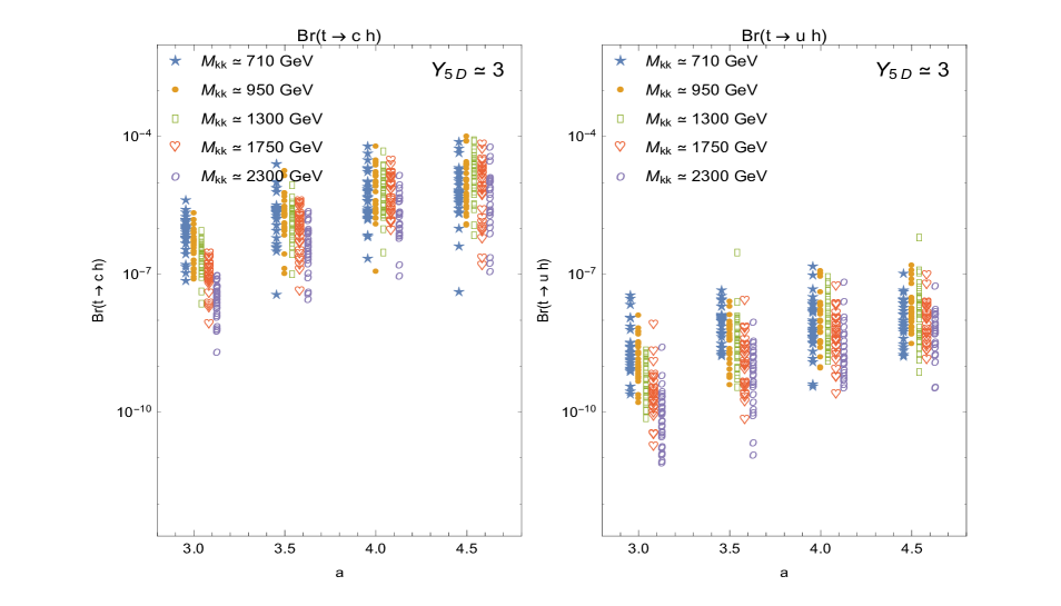
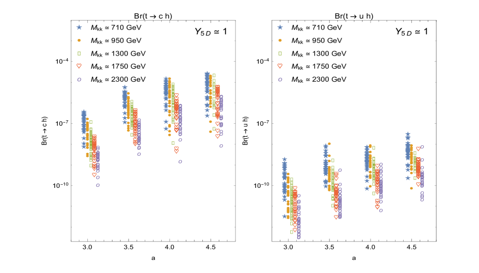
Figure 1: Branching ratios for the tree-level decays $t\to ch$ (left panels), $t\to uh$ (right panels) for four values of the Higgs localization parameter, $a\simeq\{3,3.5,4,4.5\}$. Two different 5D Yukawa average values are used, $Y^{5D}=3$ in the upper panels and $Y^{5D}=1$ in the lower panels, and five different KK gluon mass scales between $710$ GeV and $2300$ GeV set the KK scale. It is important to note that within the $Y^{5D}=1$ case, the (33) entry in the up-Yukawa matrix must still be about $\sim 3$ in order to reproduce the top quark mass.

We now proceed to analyze the other tree-level top quark FCNC decay, to the $Z$ boson, coming from terms in the Lagrangian,

$${\cal L}\ni\left(g^{u}_{U_{L,R}}{\bar{t}}_{R}\gamma_{\mu}c_{R}+g^{u}_{Q_{L,R}}{\bar{t}}_{L}\gamma_{\mu}c_{L}\right)Z^{\mu}.$$ (18)

In order to obtain the couplings in the mass basis, we must calculate first the following overlap integrals in the gauge basis, among left handed and right handed KK fermions and the $Z$ boson wavefunction,

$$(g^{u}_{Q_{L,R}})_{ij}=\frac{g^{5D}_{L,R}}{\sqrt{k}}\int_{0}^{y_{1}}dye^{-3A(y)}f_{Z}(y)Q^{m,i}_{L,R}(y)Q^{n,j}_{L,R}(y),$$ (19)

$$(g^{u}_{U_{L,R}})_{ij}=\frac{g^{5D}_{L,R}}{\sqrt{k}}\int_{0}^{y_{1}}dye^{-3A(y)}f_{Z}(y)U^{m,i}_{L,R}(y)U^{n,j}_{L,R}(y),$$ (20)

where as usual $Q^{n,j}_{L,R}(y)$ stands for the $SU(2)$ doublets and $U^{n,j}_{L,R}(y)$ for $SU(2)$ singlets. We then need to perform a rotation on the quark fields to transform to the physical mass basis. This rotation will produce tree-level flavor violating couplings of the $Z$ boson. The profile $f_{Z}(y)$ is the solution to the following differential equation

$$\partial_{y}\left(e^{-2A(y)}\partial_{y}f_{Z}(y)\right)-M_{A}^{2}f_{Z}(y)+m^{2}f_{Z}=0$$ (21)

with $M_{Z}(y)=\displaystyle{g^{5D}\over 2\cos\theta_{W}}h(y)e^{-A(y)}$ being the $y$ dependent bulk mass of the field. The $g^{5D}_{L,R}$ coupling are given by

$$g^{5D}_{L}={g^{5D}\over\cos\theta_{W}}\left(T_{3}-Q_{q}\sin^{2}\theta_{W}\right)$$

$$g^{5D}_{R}={g^{5D}\over\cos\theta_{W}}Q_{q}\sin^{2}\theta_{W},$$

with $Q_{q}$ the charge of the quark, (here ${2\over 3}$), $\theta_{W}$ the Weinberg angle and $T_{3}={1\over 2}$. Once in the mass basis we extract the flavor violating couplings $(g^{u}_{L})_{qt}$ and $(g^{u}_{R})_{qt}$ between right handed and left handed quarks and the $Z$ boson and with these, the flavor violating branching ratio is given by Casagrande:2008hr

$${\cal B}(t\rightarrow qZ)={2\left(1-r_{Z}\right)^{2}\left(2r_{Z}+1\right)\over\left(1-r_{W}\right)^{2}\left(2r_{W}+1\right)}\left(\left|(g^{u}_{L})_{\text{qt}}\right|^{2}+\left|(g^{u}_{R})_{\text{qt}}\right|^{2}-{12\sqrt{r_{q}}r_{Z}\over\left(1-r_{Z}\right)\left(2r_{Z}+1\right)}{\text{R}e}\left[(g^{u}_{L})^{*}_{\text{qt}}(g^{u}_{R})_{\text{qt}}\right]\right).$$ (22)

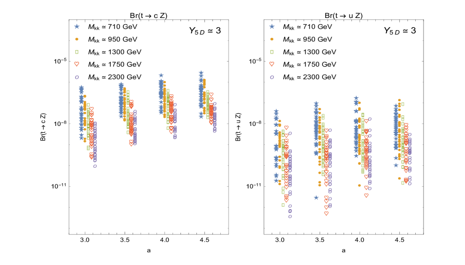
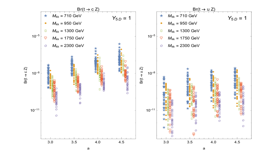
Figure 2: Branching ratios for the tree-level decays $t\to cZ$ (left panels), $t\to uZ$ (right panels) for the Higgs localization parameter, $a\in\{a_{\text{m}in},a_{\text{m}in}+0.5,a_{\text{m}in}+1,a_{\text{m}in}+1.5\}$, where $a_{\text{m}in}\simeq 3$. We have presented our results for two different scales of 5D Yukawa couplings, $Y^{5D}=1,3$ ($Y^{5D}=3$ in the upper panels, and for $Y^{5D}=1$ in the lower panels), and five different KK gluon mass scales between $710$ GeV to $2300$ GeV.

Our results are presented in Fig. 2, where again the branching ratio is expected to scale as $\displaystyle{\cal B}(t\rightarrow qZ)\propto\frac{Y^{4}}{M_{KK}^{4}}\frac{m_{q}}{v}$, although in this case there will not be a flavor cumulative effect as in the Higgs case Azatov:2009na , and so the overall effect is expected to be smaller than the flavor violating top decay into a Higgs. We observe that the $Y^{5D}=1$ and $Y^{5D}=3$ graphs show very similar branching ratios for the same values of $a$ and given KK scale. This is consistent with the fact that even in the $Y^{5D}=1$ case, there is still one large Yukawa entry, ($Y^{5D}_{33}\sim 3$). That single term must dominate the overall effect, so that both Yukawa scenarios give similar results (i.e. the rest of 5D Yukawa couplings do not seem to add up constructively as they did in the flavor violating Higgs couplings case).

The KK scale dependence is as expected, i.e. the suppression due to larger KK masses scales down consistently, so that masses 3 times heavier, produce a branching ratio about 2 orders of magnitude smaller. Finally the flavor dependence between charm and up quark also seems consistent as there should be (very roughly) some factor of $m_{u}/m_{c}$ between the flavor violating decay branching of $t\to cZ$ over that of $t\to uZ$.

III.2 Flavor-violating radiative decays of the top quark: $t\to q\gamma$ and $t\to qg$

The SM predicted values for the ${\cal B}(t\to c\gamma)$ and ${\cal B}(t\to cg)$ are far from the LHC sensitivity. As the expected sensitivity to reach the branching ratio of $t\to cg,t\to c\gamma$ at the LHC is $10^{-5}-10^{-6}$, observing these decays would also indicate an important evidence of physics beyond the SM. These flavor violating interactions are described by the following effective Lagrangian

$${\cal L}_{FCNC} = i\sum\limits_{q}\{{\bar{q}}\left(C_{8g}^{L}P_{L}+C_{8g}^{R}P_{R}\right){\sigma_{\mu\nu}q^{\nu}}tT^{a}G^{a\,\mu}\}+h.c.$$ (23)

$$+ i\sum\limits_{q}\{{\bar{q}}\left(C_{7\gamma}^{L}P_{L}+C_{7\gamma}^{R}P_{R}\right){\sigma_{\mu\nu}q^{\nu}}tA^{\mu}\}+h.c.\,.$$

The Feynman diagrams for this processes are shown in Fig. 3 for ($t\to c\gamma$), and in Fig. 4 for ($t\to cg$), and the analytical expressions needed for the calculation of the branching ratio are given in the Appendix (Section V).

$\begin{array}[]{cc}\includegraphics[height=142.26378pt]{./diag1.pdf}&\includegraphics[height=142.26378pt]{./diag2.pdf}\\ \includegraphics[height=142.26378pt]{./diag3.pdf}&\includegraphics[height=113.81102pt]{./diag4.pdf}\end{array}$

Figure 3: Feynman Diagrams for the decay $t\to c\gamma$ in warped extra dimensional models. The label (KK) implies summation over the zero and the KK modes, while KK only indicates that only KK modes contribute.

$\begin{array}[]{cc}\includegraphics[height=142.26378pt]{./diag5.pdf}&\includegraphics[height=142.26378pt]{./diag6.pdf}\\ \includegraphics[height=142.26378pt]{./diag7.pdf}&\includegraphics[height=113.81102pt]{./diag8.pdf}\end{array}$

Figure 4: Feynman Diagrams for the decay $t\to cg$ in warped extra dimensional models. The label (KK) implies summation over the zero and the KK modes, while KK only indicates that only KK modes contribute.

The scenario contains a tower of physical neutral scalars coming from the real component of the 5D Higgs doublet. There is also a tower of physical charged scalars, which contain a mixture of the charged component of the 5D Higgs doublet and the fifth component of charged 5D gauge boson (although for simplicity we will refer to them as charged KK Higgses). Finally there is a further tower of neutral CP-odd scalars, containing a mixture of the CP-odd component of the 5D Higgs doublet and the fifth component of neutral 5D gauge boson. The scenario contains also towers of charged and neutral Goldstone bosons, orthogonal admixtures of the previous 5D Higgs and gauge boson degrees of freedom (see for example Cabrer:2011fb for details).

In the calculation of loop effects we consider the truncated tower of the first 3 KK neutral Higgs modes (CP even and odd) as well as the first 3 KK charged Higgs modes, each coupled with the first 3 KK mode fermions (i.e.,  four modes in total, including the zero mode). The neutral Higgs couplings are the same as the ones given in Eq. (11) but we need to compute also the Yukawa couplings between fermions and KK Higgs modes

$$(Y_{u})_{ij}^{H_{k}}=\frac{Y^{u,5D}_{ij}}{\sqrt{k}}\int_{0}^{y_{1}}dye^{-4A(y)}h^{H_{k}}(y)Q^{m,i}_{L,R}(y)U^{n,j}_{R,L}(y),$$ (24)

constructing the corresponding ($21\times 21$) matrices in the same basis. These must then be rotated as in Section III to be transformed into the mass basis.

In the case of the charged KK Higgs couplings we have the following coupling matrices written in the same basis as the rest of Yukawa matrices

$${\bf Y}^{H_{k}^{+}LR}=\left(\begin{array}[]{ccc}(y^{H^{+}}_{u})_{3\times 3}&(0)_{3\times 3N}&(Y^{H^{+}qU})_{3\times 3N}\\ (Y^{H^{+}Qu})_{3N\times 3}&(0)_{3N\times 3N}&(Y^{H^{+}Q_{L}U_{R}})_{3N\times 3N}\\ (0)_{3N\times 3}&(Y^{H^{+}D_{L}Q_{R}})_{3N\times 3N}&(0)_{3N\times 3N}\end{array}\right),$$ (25)

and

$${\bf Y}^{H_{k}^{+}RL}=\left(\begin{array}[]{ccc}(y^{H^{+}}_{d})_{3\times 3}&(0)_{3\times 3N}&(Y^{H^{+}qD})_{3\times 3N}\\ (Y^{H^{+}Qd})_{3N\times 3}&(0)_{3N\times 3N}&(Y^{H^{+}Q_{L}D_{R}})_{3N\times 3N}\\ (0)_{3N\times 3}&(Y^{H^{+}U_{L}Q_{R}})_{3N\times 3N}&(0)_{3N\times 3N}\end{array}\right),$$ (26)

where the submatrices are obtained by evaluating the overlap integrals

$$y_{u}^{H^{+}} = \frac{(Y^{5D}_{u})_{ij}}{\sqrt{k}}\int_{0}^{y_{1}}dye^{-4A(y)}\xi^{k}(y)q^{0,i}_{L}(y)u^{0,j}_{R}(y)$$ (27)

$$Y^{H^{+}qU} = \frac{(Y_{u}^{5D})_{ij}}{\sqrt{k}}\int_{0}^{y_{1}}dye^{-4A(y)}\xi^{k}(y)q^{0,i}_{L}(y)U^{n,j}_{R}(y)$$ (28)

$$Y^{H^{+}Qu} = \frac{(Y_{u}^{5D})_{ij}}{\sqrt{k}}\int_{0}^{y_{1}}dye^{-4A(y)}\xi^{k}(y)Q^{m,i}_{L}(y)u^{0,j}_{R}(y)$$ (29)

$$Y^{H^{+}Q_{L}U_{R}} = \frac{(Y_{u}^{5D})_{ij}}{\sqrt{k}}\int_{0}^{y_{1}}dye^{-4A(y)}\xi^{k}(y)Q^{m,i}_{L}(y)U^{n,j}_{R}(y)$$ (30)

$$Y^{H^{+}Q_{R}D_{L}} = \frac{(Y_{d}^{5D})^{*}_{ij}}{\sqrt{k}}\int_{0}^{y_{1}}dye^{-4A(y)}\xi^{k}(y)Q^{m,i}_{R}(y)D^{n,j}_{L}(y)\,,$$ (31)

and

$$y_{d}^{H^{+}} = \frac{(Y^{5D}_{d})_{ij}}{\sqrt{k}}\int_{0}^{y_{1}}dye^{-4A(y)}\xi^{k}(y)q^{0,i}_{L}(y)d^{0,j}_{R}(y)$$ (32)

$$Y^{H^{+}qD} = \frac{(Y_{d}^{5D})_{ij}}{\sqrt{k}}\int_{0}^{y_{1}}dye^{-4A(y)}\xi^{k}(y)q^{0,i}_{L}(y)D^{n,j}_{R}(y)$$ (33)

$$Y^{H^{+}Qd} = \frac{(Y_{d}^{5D})_{ij}}{\sqrt{k}}\int_{0}^{y_{1}}dye^{-4A(y)}\xi^{k}(y)Q^{m,i}_{L}(y)d^{0,j}_{R}(y)$$ (34)

$$Y^{H^{+}Q_{L}D_{R}} = \frac{(Y_{d}^{5D})_{ij}}{\sqrt{k}}\int_{0}^{y_{1}}dye^{-4A(y)}\xi^{k}(y)Q^{m,i}_{L}(y)D^{n,j}_{R}(y)$$ (35)

$$Y^{H^{+}Q_{R}U_{L}} = \frac{(Y_{u}^{5D})^{*}_{ij}}{\sqrt{k}}\int_{0}^{y_{1}}dye^{-4A(y)}\xi^{k}(y)Q^{m,i}_{R}(y)U^{n,j}_{L}(y)\,.$$ (36)

We then need to transform into the physical mass basis, by appropriately rotating from the left and the right using the two different rotation matrices required to diagonalize the up mass matrix and the down mass matrix. With this procedure, the first matrix will generate the interactions $H^{+}d_{L}u_{R}$ and the second one will produce the terms $H^{+}u_{L}d_{R}$.

For the KK gluon contributions to the loop, we compute the kinetic overlap integrals similar to the ones for the $Z$ boson couplings, Eqs. (19) and (20), but with the KK gluon fields replacing the $Z$ fields.

$$\chi_{L}^{G^{k}Q^{i}Q^{j}} = \frac{g^{5D}}{\sqrt{k}}\int_{0}^{y_{1}}dye^{-3A(y)}f_{G}^{k}(y){Q}^{i}_{L}(y){Q}^{j}_{L}(y),$$ (37)

$$\chi_{L}^{G^{k}U^{i}U^{j}} = \frac{g^{5D}}{\sqrt{k}}\int_{0}^{y_{1}}dye^{-3A(y)}f_{G}^{k}(y){U}^{i}_{L}(y){U}^{j}_{L}(y),$$ (38)

$$\chi_{R}^{G^{k}Q^{i}Q^{j}} = \frac{g^{5D}}{\sqrt{k}}\int_{0}^{y_{1}}dye^{-3A(y)}f_{G}^{k}(y){Q}^{i}_{R}(y){Q}^{j}_{R}(y),$$ (39)

$$\chi_{R}^{G^{k}U^{i}U^{j}} = \frac{g^{5D}}{\sqrt{k}}\int_{0}^{y_{1}}dye^{-3A(y)}f_{G}^{k}(y){U}^{i}_{R}(y){U}^{j}_{R}(y),$$ (40)

where $g^{5D}=\sqrt{4\pi\alpha_{S}y_{1}}$.

With these matrix elements we can compute the $t\rightarrow q\gamma$ and $t\to qg$ decay rates given in V. The results of the numerical computations are presented in Figs. 5 and 6.

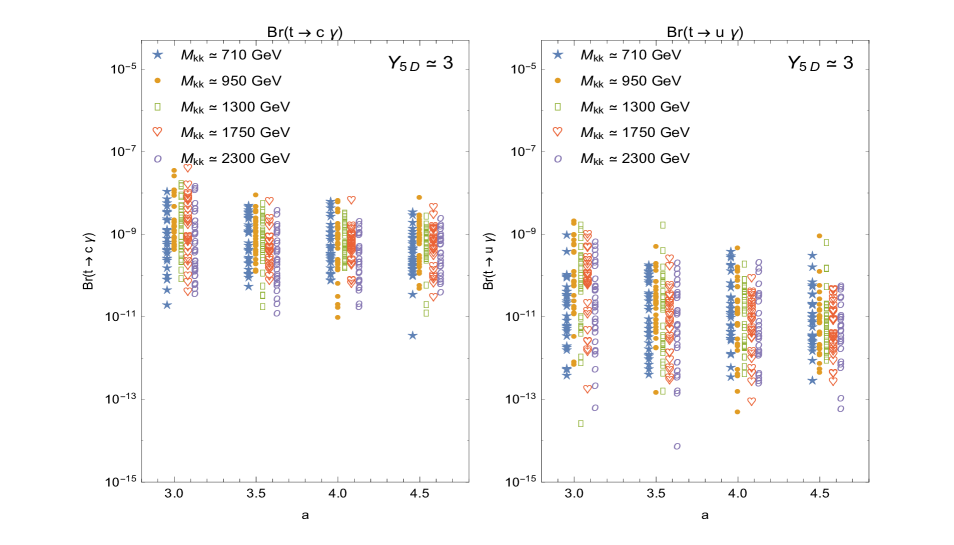
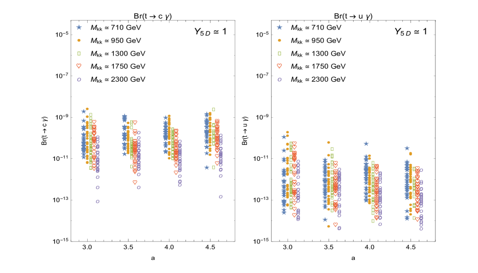
Figure 5: Branching ratios for the decays $t\to c\gamma$ (left panels) and $t\to u\gamma$ (right panels) for the the Higgs localization parameter $a$. We have presented our results for two different scales of 5D Yukawa couplings, $Y^{5D}=1,3$ ($Y^{5D}=3$ in the upper panels, and for $Y^{5D}=1$ in the lower panels), and five different KK gluon mass scales between $710$ GeV to $2300$ GeV.

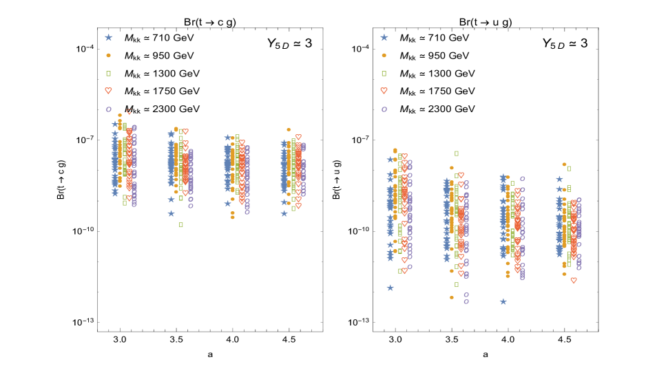
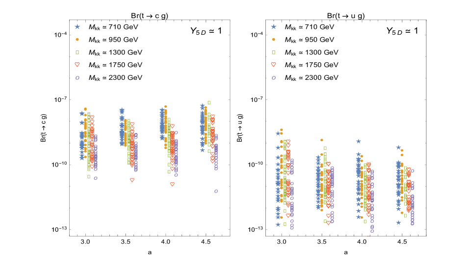
Figure 6: Branching ratios for the decay $t\to cg$ (left panels) and $t\to ug$ (right panels) for the the Higgs localization parameter $a$. We have presented our results for two different scales of 5D Yukawa couplings, $Y^{5D}=1,3$ ($Y^{5D}=3$ in the upper panels, and for $Y^{5D}=1$ in the lower panels), and five different KK gluon mass scales between $710$ GeV to $2300$ GeV.

We observe that the decay branching ratios are at most $10^{-7}$ for $t\to cg$ and $10^{-8}$ for $t\to c\gamma$, and these obtained with very light KK gluon masses of about $700$ GeV (KK Higgs are heavier). In any case, the sensitivity at the LHC for the $t\to qg$ decay is expected to be at about $\sim 10^{-5}$ which renders these results still too small to be observed.

We also observe that the expected behavior for heavier and heavier masses is not completely apparent, specially for large Yukawa couplings and large values of the Higgs parameter $a$. First of all, as we mentioned in Sec. III.1 the validity of our perturbative approach becomes questionable for larger values of Yukawa couplings and of the $a$ parameter, which, when including the flavor family effects, could start to fail for i.e.,  $Y^{5D}\simeq 3$ and for IR localized Higgs field, $a>4$ (i.e.,  for those parameters one should include another full KK level of fields to improve the situation assuming that we have not reached the strong coupling limit). In the loop calculations for $t\rightarrow q\gamma$ and $t\to qg$ this effect might be partly at play in the most extreme regions of the parameter space shown and one should therefore look at the results presented for large Yukawa couplings and large values of $a$ as being close to the limit of validity of our approach.

Nevertheless, there seems to be also a specific characteristic behavior of the scenario at play here. After scanning the parameter space, in all loop evaluations, it appears that the Higgs and KK Higgs contributions to the loop are larger than the KK gluon contributions by one order of magnitude. This should be in part responsible for the fact that the loop processes do not appear very sensitive to the KK mass scale. The reason for this is that the mass scale indicated on the plots represents the lowest KK gluon mass, while the computed KK Higgs masses are always larger and less sensitive to changes in the KK volume as the KK gluons, in the first portion of parameter range. In particular, when the lightest KK gluon is $710$ GeV, the lightest KK Higgs is $\sim 1300$ GeV, while when the KK gluon mass is $950$ GeV, the lightest KK Higgs remains at $\sim 1300$ GeV. When the KK gluon mass is increased to $1300$ GeV, the lowest KK Higgs mass becomes $1500$ GeV, and from then on, the increases in masses remain relatively similar. This means that the effect expected from changing the KK scale is milder since the lightest KK Higgs have similar masses despite increasingly heavier KK gluons, thus obscuring the mass scale dependence (as the loops are dominated by the KK Higgs).

IV Summary and Conclusion

We presented a comprehensive analysis of FCNC decays of the top quark, both at tree-level and one-loop, in the context of a general warped extra dimensional space scenario, with all the fields in the bulk, such that a low KK scale is allowed without violating electroweak precision constraints.

We first constructed a complete KK tower of scalar, fermion and gauge boson states, consistent with the experimental data. We imposed constraints on the masses and mixing of zero-mode fermions so as to be consistent with the known quark masses and the CKM mixing matrix, and therefore limiting the possible values of the fermion localization parameters $c_{i}$. We used the fermion and scalar profiles to analyze the FCNC branching ratios of the top quark, both at tree and one-loop level, as functions of the Higgs localization parameter $a$ (bulk localized Higgs) and for various KK scales, allowing the 5D Yukawa couplings for the quarks to be of order $Y^{5D}=1$ and $Y^{5D}=3$. We performed all our calculations in the mass eigenstate basis, where we can take into account quark inter-generational mixing. This involved diagonalizing the $21\times 21$ dimensional fermion matrices and rotating various $21\times 21$ Yukawa coupling matrices and KK gauge-fermion-fermion matrices.

The most promising of these decays is the tree-level $t\to ch$, whose branching ratio could reach ${\cal O}(10^{-5})$ and thus become observable at the LHC @13 TeV. We note that while the branching ratio is slightly higher for $Y^{5D}=3$ (which might reach the non-perturbativity limit, particularly for highly IR localized Higgs), it is still of the same order of magnitude as for $Y^{5D}=1$ (in this case, most of the Yukawa couplings are ${\cal O}(1)$, but there must always be a larger than normal Yukawa entry, $Y^{5D}_{33}\sim 3$, in order to reproduce the top quark mass). The tree-level decay $t\to cZ$ is, as expected, a couple of orders of magnitude smaller, as it is driven by kinetic mixing rather than Yukawa couplings. At one-loop level the branching ratio for the decay $t\to c\gamma$ can be at most of ${\cal O}(10^{-8})$, and the one for $t\to cg$ an order of magnitude larger. Both of these contributions are dominated by the presence of Higgs and KK Higgs in the loops, rather than loops with KK gluons. The dependence with the KK gluon mass scale is more pronounced for the tree-level decays, while in the loop decays the decoupling with respect to the KK mass is less apparent, specially for large Yukawa couplings and large Higgs localization parameter $a$. This can be due to the parameter space points approaching a non-perturbative regime, but it is also partly due to the fact that the KK Higgs masses happen to change less rapidly than the KK gluon masses as we change the background parameters in order to increase the KK scale.

In summary, a comprehensive analysis of top flavor-changing neutral decays in general warped extra dimensional models indicates that the only decay with a chance to be observed is the tree-level decay $t\to ch$, while the loop-level decays $t\to c\gamma$ and $t\to cg$ seem to fall well below the sensitivity of LHC @ 13 or 14 TeV.

V Appendix

We include here, for completeness the analytical expressions for the loop calculations presented in III.2.

V.0.1 $t\to q\gamma$, Higgs loop contributions, zero mode and KK

For $t_{R}$, charged Higgs

$$F_{T_{R}}^{\gamma\,+} = \frac{e}{16\pi^{2}}\sum\limits_{i=0}^{nKK}\sum\limits_{j=0}^{mKK}\frac{1}{M_{H^{+}_{i}}^{2}}\Bigg{\{}\left[m_{t}\left(Y^{H_{i}^{+}t_{R}D_{j}}\right)\left(Y^{H_{i}^{+}c_{R}D_{j}}\right)^{\star}+m_{c}\left(Y^{H_{i}^{+}t_{L}D_{j}}\right)\left(Y^{H_{i}^{+}c_{L}D_{j}}\right)^{\star}\right]$$

$$\times \left[-\frac{1}{3}f_{1}(x_{ji})+g_{1}(x_{ji})\right]+\left[M_{D_{j}}\left(Y^{H_{i}^{+}t_{L}D_{j}}\right)\left(Y^{H_{i}^{+}c_{R}D_{j}}\right)^{\star}\right]\times\left[-\frac{1}{3}f_{2}(x_{ji})+g_{2}(x_{ji})\right]\Bigg{\}}\,.$$

For $t_{L}$, charged Higgs

$$F_{T_{L}}^{\gamma\,+} = \frac{e}{16\pi^{2}}\sum\limits_{i=0}^{nKK}\sum\limits_{j=0}^{mKK}\frac{1}{M_{H^{+}_{i}}^{2}}\Bigg{\{}\left[m_{c}\left(Y^{H_{i}^{+}t_{R}D_{j}}\right)\left(Y^{H_{i}^{+}c_{R}D_{j}}\right)^{\star}+m_{t}\left(Y^{H_{i}^{+}t_{L}D_{j}}\right)\left(Y^{H_{i}^{+}c_{L}D_{j}}\right)^{\star}\right]$$

$$\times \left[-\frac{1}{3}f_{1}(x_{ji})+g_{1}(x_{ji})\right]+\left[M_{D_{j}}\left(Y^{H_{i}^{+}t_{R}D_{j}}\right)\left(Y^{H_{i}^{+}c_{L}D_{j}}\right)^{\star}\right]\times\left[-\frac{1}{3}f_{2}(x_{ji})+g_{2}(x_{ji})\right]\Bigg{\}}\,,$$

where we used $\displaystyle x_{ji}=\frac{M^{2}_{D_{j}}}{M^{2}_{H^{+}_{i}}}$ and $nKK$ is the number of Higgs modes included, $mKK$ is the number of fermion modes included for each flavor.

For $t_{R}$, neutral Higgs

$$F_{T_{R}}^{\gamma\,0} = \frac{e}{16\pi^{2}}\sum\limits_{i=0}^{nKK}\sum\limits_{j=0}^{mKK}\frac{1}{M_{H^{0}_{i}}^{2}}\Bigg{\{}\left[m_{t}\left(Y^{H_{i}^{0}t_{R}U_{j}}\right)\left(Y^{H_{i}^{0}c_{R}U_{j}}\right)^{\star}+m_{c}\left(Y^{H_{i}^{0}t_{L}U_{j}}\right)\left(Y^{H_{i}^{0}c_{L}U_{j}}\right)^{\star}\right]$$

$$\times \left[\frac{2}{3}f_{1}(y_{ji})\right]+\left[M_{U_{j}}\left(Y^{H_{i}^{0}t_{L}U_{j}}\right)\left(Y^{H_{i}^{0}c_{R}U_{j}}\right)^{\star}\right]\times\left[\frac{2}{3}f_{2}(y_{ji})\right]\Bigg{\}}\,.$$

For $t_{L}$, neutral Higgs

$$F_{T_{L}}^{\gamma\,0} = \frac{e}{16\pi^{2}}\sum\limits_{i=0}^{nKK}\sum\limits_{j=0}^{mKK}\frac{1}{M_{H^{0}_{i}}^{2}}\Bigg{\{}\left[m_{c}\left(Y^{H_{i}^{0}t_{R}U_{j}}\right)\left(Y^{H_{i}^{0}c_{R}U_{j}}\right)^{\star}+m_{t}\left(Y^{H_{i}^{0}t_{L}U_{j}}\right)\left(Y^{H_{i}^{0}c_{L}U_{j}}\right)^{\star}\right]$$

$$\times \left[\frac{2}{3}f_{1}(y_{ji})\right]+\left[M_{U_{j}}\left(Y^{H_{i}^{0}t_{R}U_{j}}\right)\left(Y^{H_{i}^{0}c_{L}U_{j}}\right)^{\star}\right]\times\left[\frac{2}{3}f_{2}(y_{ji})\right]\Bigg{\}}\,,$$

where we used $\displaystyle y_{ji}=\frac{M^{2}_{U_{j}}}{M^{2}_{H^{0}_{i}}}$.

V.0.2 $t\to q\gamma$, KK Gluon Loop Contributions

$$F_{T_{R}}^{\gamma\,G} = C(R)\frac{e}{16\pi^{2}}\sum\limits_{i=0}^{nKK}\sum\limits_{j=0}^{mKK}\frac{1}{M_{G_{i}}^{2}}\Bigg{\{}\left[m_{t}\left(\chi^{G_{i}U_{j}c_{L}}\right)^{\dagger}\left(\chi^{G_{i}U_{j}t_{L}}\right)f_{1}(x_{ji})+M_{U_{j}}\left(\chi^{G_{i}U_{j}c_{L}}\right)^{\dagger}\left(\chi^{G_{i}U_{j}t_{R}}\right)g_{1}(x_{ji})\right]\Bigg{\}}\,,$$

$$F_{T_{L}}^{\gamma\,G} = C(R)\frac{e}{16\pi^{2}}\sum\limits_{i=0}^{nKK}\sum\limits_{j=0}^{mKK}\frac{1}{M_{G_{i}}^{2}}\Bigg{\{}\left[m_{t}\left(\chi^{G_{i}U_{j}c_{R}}\right)^{\dagger}\left(\chi^{G_{i}U_{j}t_{R}}\right)f_{1}(x_{ji})+M_{U_{j}}\left(\chi^{G_{i}U_{j}c_{R}}\right)^{\dagger}\left(\chi^{G_{i}U_{j}t_{L}}\right)g_{1}(x_{ji})\right]\Bigg{\}}\,,$$

where $\displaystyle x_{ji}=\frac{M^{2}_{U_{j}}}{M^{2}_{G_{i}}}$ and $\chi^{G_{i}U_{j}c(t)_{L,R}}$ are the KK gluon couplings to $c(t)$ external quarks and KK $U$ fermions, and where and $C(R)=4/3$ is the quadratic Casimir operator on the fundamental representation of $SU(3)_{c}$. We have

$$C_{7\,\gamma}^{L} = F_{T_{L}}^{\gamma\,+}+F_{T_{L}}^{\gamma\,0}+F_{T_{L}}^{\gamma\,G}\,,$$

$$C_{7\,\gamma}^{R} = F_{T_{R}}^{\gamma\,+}+F_{T_{R}}^{\gamma\,0}+F_{T_{R}}^{\gamma\,G}\,,$$

and

$$\Gamma(t\to c\gamma)=\frac{m^{3}_{t}}{16\pi}\left(|C_{7\,\gamma}^{L}|^{2}+|C_{7\,\gamma}^{R}|^{2}\right)\,.$$ (46)

V.0.3 $t\to qg$, Higgs loop contributions, zero mode and KK

For $t_{R}$, charged Higgs

$$F_{T_{R}}^{g\,+} = \frac{g_{s}}{16\pi^{2}}\sum\limits_{i=0}^{nKK}\sum\limits_{j=0}^{mKK}\frac{1}{M_{H^{+}_{i}}^{2}}\Bigg{\{}\left[m_{t}\left(Y^{H_{i}^{+}t_{R}D_{j}}\right)\left(Y^{H_{i}^{+}c_{R}D_{j}}\right)^{\star}+m_{c}\left(Y^{H_{i}^{+}t_{L}D_{j}}\right)\left(Y^{H_{i}^{+}c_{L}D_{j}}\right)^{\star}\right]f_{1}(x_{ji})$$ (47)

$$+ \left[M_{D_{j}}\left(Y^{H_{i}^{+}t_{L}D_{j}}\right)\left(Y^{H_{i}^{+}c_{R}D_{j}}\right)^{\star}\right]f_{2}(x_{ji})\Bigg{\}}\,.$$

For $t_{L}$, charged Higgs

$$F_{T_{L}}^{g\,+} = \frac{g_{s}}{16\pi^{2}}\sum\limits_{i=0}^{nKK}\sum\limits_{j=0}^{mKK}\frac{1}{M_{H^{+}_{i}}^{2}}\Bigg{\{}\left[m_{c}\left(Y^{H_{i}^{+}t_{R}D_{j}}\right)\left(Y^{H_{i}^{+}c_{R}D_{j}}\right)^{\star}+m_{t}\left(Y^{H_{i}^{+}t_{L}D_{j}}\right)\left(Y^{H_{i}^{+}c_{L}D_{j}}\right)^{\star}\right]f_{1}(x_{ji})$$ (48)

$$+ \left[M_{D_{j}}\left(Y^{H_{i}^{+}t_{R}D_{j}}\right)\left(Y^{H_{i}^{+}c_{L}D_{j}}\right)^{\star}\right]f_{2}(x_{ji})\Bigg{\}}\,,$$

where as before $\displaystyle x_{ji}=\frac{M^{2}_{D_{j}}}{M^{2}_{H^{+}_{i}}}$ and $nKK$ is the number of Higgs modes included, $mKK$ is the number of fermion modes included for each flavor.

For $t_{R}$, neutral Higgs

$$F_{T_{R}}^{g\,0} = \frac{g_{s}}{16\pi^{2}}\sum\limits_{i=0}^{nKK}\sum\limits_{j=0}^{mKK}\frac{1}{M_{H^{0}_{i}}^{2}}\Bigg{\{}\left[m_{t}\left(Y^{H_{i}^{0}t_{R}U_{j}}\right)\left(Y^{H_{i}^{0}c_{R}U_{j}}\right)^{\star}+m_{c}\left(Y^{H_{i}^{0}t_{L}U_{j}}\right)\left(Y^{H_{i}^{0}c_{L}U_{j}}\right)^{\star}\right]f_{1}(y_{ji})$$ (49)

$$+ \left[M_{U_{j}}\left(Y^{H_{i}^{0}t_{L}U_{j}}\right)\left(Y^{H_{i}^{0}c_{R}U_{j}}\right)^{\star}\right]f_{2}(y_{ji})\Bigg{\}}\,.$$

For $t_{L}$, neutral Higgs

$$F_{T_{L}}^{g\,0} = \frac{g_{s}}{16\pi^{2}}\sum\limits_{i=0}^{nKK}\sum\limits_{j=0}^{mKK}\frac{1}{M_{H^{0}_{i}}^{2}}\Bigg{\{}\left[m_{c}\left(Y^{H_{i}^{0}t_{R}U_{j}}\right)\left(Y^{H_{i}^{0}c_{R}U_{j}}\right)^{\star}+m_{t}\left(Y^{H_{i}^{0}t_{L}U_{j}}\right)\left(Y^{H_{i}^{0}c_{L}U_{j}}\right)^{\star}\right]f_{1}(y_{ji})$$ (50)

$$+ \left[M_{U_{j}}\left(Y^{H_{i}^{0}t_{R}U_{j}}\right)\left(Y^{H_{i}^{0}c_{L}U_{j}}\right)^{\star}\right]f_{2}(y_{ji})\Bigg{\}}\,,$$

where as before $\displaystyle y_{ji}=\frac{M^{2}_{U_{j}}}{M^{2}_{H^{0}_{i}}}$.

V.0.4 $t\to qg$, KK Gluon Loop Contributions

$$F_{T_{R}}^{g\,G} = \frac{g_{s}}{16\pi^{2}}\sum\limits_{i=0}^{nKK}\sum\limits_{j=0}^{mKK}\frac{1}{M_{G_{i}}^{2}}\Bigg{\{}m_{t}\left(\chi^{G_{i}U_{j}c_{L}}\right)^{\dagger}\left(\chi^{G_{i}U_{j}t_{L}}\right)\left[-C(G)f_{1}(x_{ji})+\left(2C(R)-C(G)\right)f_{2}(x_{ji})\right]$$

$$+ M_{U_{j}}\left(\chi^{G_{i}U_{j}c_{L}}\right)^{\dagger}\left(\chi^{G_{i}U_{j}t_{R}}\right)\left[-C(G)g_{2}(x_{ji})+\left(2C(R)-C(G)\right)g_{1}(x_{ji})\right]\Bigg{\}}\,,$$

$$F_{T_{L}}^{g\,G} = \frac{g_{s}}{16\pi^{2}}\sum\limits_{i=0}^{nKK}\sum\limits_{j=0}^{mKK}\frac{1}{M_{G_{i}}^{2}}\Bigg{\{}m_{t}\left(\chi^{G_{i}U_{j}c_{R}}\right)^{\dagger}\left(\chi^{G_{i}U_{j}t_{R}}\right)\left[-C(G)f_{1}(x_{ji})+\left(2C(R)-C(G)\right)f_{2}(x_{ji})\right]$$ (51)

$$+ M_{U_{j}}\left(\chi^{G_{i}U_{j}c_{R}}\right)^{\dagger}\left(\chi^{G_{i}U_{j}t_{L}}\right)\left[-C(G)g_{2}(x_{ji})+\left(2C(R)-C(G)\right)g_{1}(x_{ji})\right]\Bigg{\}}\,,$$

where $\displaystyle x_{ji}=\frac{M^{2}_{U_{j}}}{M^{2}_{G_{i}}}$ and $\chi^{G_{i}U_{j}c(t)_{L,R}}$ are the KK gluon couplings to $c(t)$ external quarks and KK $U$ fermions, and where and $C(G)=3$ and $C(R)=4/3$ are the quadratic Casimir operator on the adjoint and fundamental representation of $SU(3)_{c}$, respectively.

We have

$$C_{8\,g}^{L} = F_{T_{L}}^{g\,+}+F_{T_{L}}^{g\,0}+F_{T_{L}}^{g\,G}\,,$$

$$C_{8\,g}^{R} = F_{T_{R}}^{g\,+}+F_{T_{R}}^{g\,0}+F_{T_{R}}^{g\,G}\,,$$

and

$$\Gamma(t\to cg)=\frac{m^{3}_{t}}{16\pi}\left(|C_{8\,g}^{L}|^{2}+|C_{8\,g}^{R}|^{2}\right)\,.$$ (52)

The loop functions in the above expressions are:

$$f_{1}(x) = -\frac{x^{3}-6x^{2}+3x+2+6x\ln x}{12(x-1)^{4}}\,,$$ (53)

$$f_{2}(x) = -\frac{x^{2}-4x+3+2\ln x}{2(x-1)^{3}}\,,$$ (54)

$$g_{1}(x) = \frac{2x^{3}+3x^{2}-6x+1-6x^{2}\ln x}{12(x-1)^{4}}\,,$$ (55)

$$g_{2}(x) = \frac{x^{2}-1-2x\ln x}{2(x-1)^{3}}\,.$$ (56)

References

• (1) L. Randall and R. Sundrum, Phys. Rev. Lett.  83, 4690 (1999); L. Randall and R. Sundrum, Phys. Rev. Lett.  83, 3370 (1999).
• (2) Y. Grossman and M. Neubert, Phys. Lett. B 474, 361 (2000); T. Gherghetta and A. Pomarol, Nucl. Phys. B 586, 141 (2000); H. Davoudiasl, J. L. Hewett and T. G. Rizzo, Phys. Lett. B 473, 43 (2000); S. Chang, J. Hisano, H. Nakano, N. Okada and M. Yamaguchi, Phys. Rev. D 62, 084025 (2000); A. Pomarol, Phys. Lett. B 486, 153 (2000).
• (3) S. J. Huber and Q. Shafi, Phys. Lett. B 498, 256 (2001); S. J. Huber, Nucl. Phys. B 666, 269 (2003); K. Agashe, G. Perez and A. Soni, Phys. Rev. D 71, 016002 (2005); C. Csaki, A. Falkowski and A. Weiler, JHEP 0809, 008 (2008); M. Blanke, A. J. Buras, B. Duling, S. Gori and A. Weiler, JHEP 0903, 001 (2009); C. Csaki, A. Falkowski and A. Weiler, JHEP 0809, 008 (2008); A. L. Fitzpatrick, G. Perez and L. Randall, Phys. Rev. Lett.  100, 171604 (2008); S. Davidson, G. Isidori and S. Uhlig, Phys. Lett.  B 663, 73 (2008).
• (4) K. Agashe, A. Belyaev, T. Krupovnickas, G. Perez and J. Virzi, Phys. Rev.  D 77, 015003 (2008); B. Lillie, L. Randall and L. T. Wang, JHEP 0709, 074 (2007); B. Lillie, J. Shu and T. M. P. Tait, Phys. Rev.  D 76, 115016 (2007); A. Djouadi, G. Moreau and R. K. Singh, Nucl. Phys.  B 797, 1 (2008); M. Guchait, F. Mahmoudi and K. Sridhar, Phys. Lett.  B 666, 347 (2008); U. Baur and L. H. Orr, Phys. Rev.  D 76, 094012 (2007); Phys. Rev.  D 77, 114001 (2008); M. Carena, A. D. Medina, B. Panes, N. R. Shah and C. E. M. Wagner, Phys. Rev.  D 77, 076003 (2008).
• (5) K. Agashe, A. Delgado, M. J. May and R. Sundrum, JHEP 0308, 050 (2003); C. Csaki, C. Grojean, L. Pilo and J. Terning, Phys. Rev. Lett.  92, 101802 (2004).
• (6) M. Carena, A. Delgado, E. Ponton, T. M. P. Tait and C. E. M. Wagner, Phys. Rev. D 71, 015010 (2005); H. Davoudiasl, J. L. Hewett and T. G. Rizzo, Phys. Rev. D 68, 045002 (2003).
• (7) A. Falkowski and M. Perez-Victoria, JHEP 0812, 107 (2008).
• (8) B. Batell, T. Gherghetta and D. Sword, Phys. Rev. D 78, 116011 (2008); T. Gherghetta and D. Sword, Phys. Rev. D 80, 065015 (2009); T. Gherghetta and N. Setzer, Phys. Rev. D 82, 075009 (2010).
• (9) J. A. Cabrer, G. von Gersdorff and M. Quiros, New J. Phys.  12, 075012 (2010). J. A. Cabrer, G. von Gersdorff and M. Quiros, Phys. Lett. B 697, 208 (2011); J. A. Cabrer, G. von Gersdorff and M. Quiros, JHEP 1105, 083 (2011); J. A. Cabrer, G. von Gersdorff and M. Quiros, Phys. Rev. D 84, 035024 (2011); J. A. Cabrer, G. von Gersdorff and M. Quiros, JHEP 1201, 033 (2012). A. Carmona and J. Santiago, JHEP 1201, 100 (2012).
• (10) A. Carmona, E. Ponton and J. Santiago, JHEP 1110, 137 (2011); S. Mert Aybat and J. Santiago, Phys. Rev. D 80, 035005 (2009); A. Delgado and D. Diego, Phys. Rev. D 80, 024030 (2009); J. de Blas, A. Delgado, B. Ostdiek and A. de la Puente, Phys. Rev. D 86, 015028 (2012).
• (11) C. Delaunay, J. F. Kamenik, G. Perez and L. Randall, JHEP 1301, 027 (2013).
• (12) K. Agashe, A. Azatov, Y. Cui, L. Randall and M. Son, JHEP 1506, 196 (2015).
• (13) J. J. Cao, G. Eilam, M. Frank, K. Hikasa, G. L. Liu, I. Turan and J. M. Yang, Phys. Rev. D 75, 075021 (2007); C. S. Li, R. J. Oakes and J. M. Yang, Phys. Rev. D 49, 293 (1994) Erratum: [Phys. Rev. D 56, 3156 (1997)]; J. L. Lopez, D. V. Nanopoulos and R. Rangarajan, Phys. Rev. D 56, 3100 (1997); G. Couture, C. Hamzaoui and H. Konig, Phys. Rev. D 52, 1713 (1995); G. M. de Divitiis, R. Petronzio and L. Silvestrini, Nucl. Phys. B 504, 45 (1997); G. Eilam, A. Gemintern, T. Han, J. M. Yang and X. Zhang, Phys. Lett. B 510, 227 (2001); J. Guasch and J. Sola, Nucl. Phys. B 562, 3 (1999); J. j. Cao, Z. h. Xiong and J. M. Yang, Nucl. Phys. B 651, 87 (2003); J. Cao, G. Eilam, K. i. Hikasa and J. M. Yang, Phys. Rev. D 74, 031701 (2006); T. Han, K. i. Hikasa, J. M. Yang and X. m. Zhang, Phys. Rev. D 70, 055001 (2004); M. Frank and I. Turan, Phys. Rev. D 72, 035008 (2005).
• (14) J. A. Aguilar-Saavedra, Acta Phys. Polon. B 35, 2695 (2004); J. A. Aguilar-Saavedra and B. M. Nobre, Phys. Lett. B 553, 251 (2003); G. Eilam, J. L. Hewett and A. Soni, Phys. Rev. D 44, 1473 (1991) [Phys. Rev. D 59, 039901 (1999)]; B. Mele, S. Petrarca and A. Soddu, Phys. Lett. B 435, 401 (1998); J. L. Diaz-Cruz, R. Martinez, M. A. Perez and A. Rosado, Phys. Rev. D 41, 891 (1990); F. Larios, R. Martinez and M. A. Perez, Int. J. Mod. Phys. A 21, 3473 (2006).
• (15) J. A. Aguilar-Saavedra, Phys. Rev. D 67, 035003 (2003) [Phys. Rev. D 69, 099901 (2004)].
• (16) D. Atwood, L. Reina and A. Soni, Phys. Rev. D 55, 3156 (1997); B. Grzadkowski, J. F. Gunion and P. Krawczyk, Phys. Lett. B 268, 106 (1991); A. Arhrib, Phys. Rev. D 72, 075016 (2005); S. Bejar, J. Guasch and J. Sola, Nucl. Phys. B 600, 21 (2001).
• (17) M. E. Luke and M. J. Savage, Phys. Lett. B 307, 387 (1993); D. Atwood, L. Reina and A. Soni, Phys. Rev. D 53, 1199 (1996); D. Atwood, L. Reina and A. Soni, Phys. Rev. Lett.  75, 3800 (1995);
• (18) J. j. Cao, G. l. Liu, J. M. Yang and H. j. Zhang, Phys. Rev. D 76, 014004 (2007); G. Burdman, Phys. Rev. Lett.  83, 2888 (1999); H. J. Zhang, Phys. Rev. D 77, 057501 (2008); G. Liu and H. j. Zhang, Chin. Phys. C 32, 697 (2008); G. L. Liu, Chin. Phys. Lett.  26, 101401 (2009).
• (19) X. F. Han, L. Wang and J. M. Yang, Phys. Rev. D 80, 015018 (2009); H. Hong-Sheng, Phys. Rev. D 75, 094010 (2007); R. Gaitan, R. Martinez and J. H. M. de Oca, arXiv:1503.04391 [hep-ph].
• (20) G. A. Gonzalez-Sprinberg, R. Martinez and J. A. Rodriguez, Eur. Phys. J. C 51, 919 (2007).
• (21) J. I. Aranda, A. Cordero-Cid, F. Ramirez-Zavaleta, J. J. Toscano and E. S. Tututi, Phys. Rev. D 81, 077701 (2010); J. I. Aranda, A. Cordero-Cid, F. Ramirez-Zavaleta, J. J. Toscano and E. S. Tututi, Mod. Phys. Lett. A 24, 3219 (2009).
• (22) C. Csaki, Y. Grossman, P. Tanedo and Y. Tsai, Phys. Rev. D 83, 073002 (2011); K. Agashe, G. Perez and A. Soni, Phys. Rev. Lett.  93, 201804 (2004): K. Agashe, A. E. Blechman and F. Petriello, Phys. Rev. D 74, 053011 (2006); M. Blanke, B. Shakya, P. Tanedo and Y. Tsai, JHEP 1208, 038 (2012); M. Beneke, P. Moch and J. Rohrwild, doi:10.1016/j.nuclphysb.2016.02.037.
• (23) T. J. Gao, T. F. Feng and J. B. Chen, JHEP 1302, 029 (2013); W. F. Chang, J. N. Ng and J. M. S. Wu, Phys. Rev. D 78, 096003 (2008).
• (24) G. Aad et al. [ATLAS Collaboration], Eur. Phys. J. C 76, no. 1, 12 (2016).
• (25) CMS Collaboration CMS-PAS-TOP-14-003.
• (26) K. Agashe et al. [Top Quark Working Group Collaboration], arXiv:1311.2028 [hep-ph].
• (27) M. Frank, N. Pourtolami and M. Toharia, Phys. Rev. D 87, no. 9, 096003 (2013).
• (28) M. Frank, N. Pourtolami and M. Toharia, Phys. Rev. D 89, no. 1, 016012 (2014).
• (29) M. Frank, N. Pourtolami and M. Toharia, Phys. Rev. D 93, no. 5, 056004 (2016).
• (30) K. Agashe, A. Azatov and L. Zhu, Phys. Rev. D 79, 056006 (2009); O. Gedalia, G. Isidori and G. Perez, Phys. Lett. B 682, 200 (2009).
• (31) A. Azatov, M. Toharia and L. Zhu, Phys. Rev. D 80, 035016 (2009).
• (32) M. Frank, C. Hamzaoui, N. Pourtolami and M. Toharia, Phys. Rev. D 91, 116001 (2015).
• (33) S. Casagrande, F. Goertz, U. Haisch, M. Neubert and T. Pfoh, JHEP 0810, 094 (2008).