Quantum phase diagram of $J_{1}-J_{2}$ Heisenberg $S=1/2$ antiferromagnet in honeycomb lattice: a modified spin wave study

Abstract

Using modified spin wave (MSW) method, we study the $J_{1}-J_{2}$ Heisenberg model with first and second neighbor antiferromagnetic exchange interactions. For symmetric $S=1/2$ model, with the same couplings for all the equivalent neighbors, we find three phase in terms of frustration parameter ${\bar{\alpha}=J_{2}/J_{1}}$: (1) a commensurate collinear ordering with staggered magnetization (Néel.I state) for $0\leq{\bar{\alpha}}\lesssim 0.207$ , (2) a magnetically gapped disordered state for $0.207\lesssim{\bar{\alpha}}\lesssim 0.369$, preserving all the symmetries of the Hamiltonian and lattice, hence by definition is a quantum spin liquid (QSL) state and (3) a commensurate collinear ordering in which two out of three nearest neighbor magnetizations are antiparallel and the remaining pair are parallel (Néel.II state), for $0.396\lesssim{\bar{\alpha}}\leq 1$. We also explore the phase diagram of distorted $J_{1}-J_{2}$ model with $S=1/2$. Distortion is introduced as an inequality of one nearest neighbor coupling with the other two. This yields a richer phase diagram by the appearance of a new gapped QSL, a gapless QSL and also a valence bond crystal (VBC) phase in addition to the previously three phases found for undistorted model.

I Introduction

Recent synthesis of compounds consisting of transition metal-oxide layers with honeycomb structure, has drawn the attentions to the magnetic properties of the spin models in honeycomb lattice. Three experimental realizations of honeycomb magnetic materials are InCu_2/3V_1/3O₃ InCuVO , Cu₃Ni₂SbO₆ CuNiSbO and Bi₃Mn₄O₁₂(NO₃) (BMNO) bmno1 . Cu⁺² ions with $S=1/2$ in the first, Ni⁺ ions with $S=1$ in the second and Mn⁺⁴ ions with $S=3/2$ in the third compound reside on the lattice points of weakly coupled honeycomb layers. InCu_2/3V_1/3O₃ develops antiferromagnetic (AF) ordering below $\sim 20$K InCuVO2 . However, for BMNO the magnetic susceptibility as well as specific heat measurements show no sign of magnetic ordering down to $T=0.4$K, in spite of the high Curie-Weiss temperature $T_{\rm CW}\approx-257$K bmno1 .

On the theoretical front, the large scale Quantum Monte Carlo (QMC) simulation of the half-filled Hubbard model on the honeycomb lattice, proposes a gapped quantum spin liquid (QSL) phase (a magnetically disordered state preserving all the symmetries of the Hamiltonian and the lattice) for intermediate values of on-site coulomb interaction between the AF-Mott insulating and the semi-metallic phases meng . Although, later QMC simulations on larger lattice sizes refuted the existence of such a QSL phase debate1 ; debate2 ; debate3 , nevertheless, many researches were devoted to the study of AF spin models in honeycomb structure katsura ; QMC ; nlsigma ; sw ; series ; fouet ; takano ; noorbakhsh ; kawamura ; Aron2010 ; sd2 ; mosadeq ; pvb2 ; pvb3 ; pvb4 ; pvb5 ; pvb6 ; pvb7 ; pvb8 ; SB-lamas1 ; SB-wang ; SF-lu ; VMC-sondhi ; SB-lamas2 ; SB-china ; eps ; ring1 ; ring2 ; zare ; bishop ; Ciolo ; DMRG-s1 ; bishop-s1 .

Since honeycomb lattice is bipartite, Heisenberg model with nearest neighbor AF interactions in the this lattice is not frustrated and develops long-range Néel ordering. However, enhanced quantum fluctuations, due to the small coordination number ($Z=3$), reduce the staggered magnetization by about half of its classical value QMC ; series ; sw ; noorbakhsh . Therefore, the expectation for realization of a QSL phase in honeycomb based magnets, requires the introduction of frustrating exchange interactions. The simplest model incorporating frustration effects on the honeycomb lattice is $J_{1}-J_{2}$ Heisenberg model, where $J_{1}>0$ and $J_{2}>0$ are nearest and next to nearest neighbor AF exchange interactions, respectively. The classical phase diagram of this model, studied by Katsura et al katsura , shows that the Néel ordered phase is stable for $J_{2}/J_{1}<1/6$. However, for $1/6<J_{2}/J_{1}<1/2$ the classical ground state becomes infinitely degenerate and can be characterized by a manifold of spiral wave vectors. Okumura et al, used the low temperature expansion and Monte Carlo (MC) simulation, to show that the such a large ground state degeneracy can be lifted by thermal fluctuations in such a way that a broken symmetry state, with three-fold ($C_{3}$) symmetry of the honeycomb lattice, would be selected kawamura . In the vicinity of AF phase boundary ($J_{2}/J_{1}\sim 1/6$), the energy scale associated with such a thermal order by disorder mechanism becomes extremely small, leading to exotic spin liquid behaviors, whereby the spin structure factor would have different pattern in comparing with the paramagnetic phase kawamura .

Order by disorder mechanism driven by quantum fluctuations has been studied by Mulder et al. They showed that the spin wave corrections lower the energy of some states with particular incommensurate wave vectors in the ground state manifold, for the classically degenerate region $1/6<J_{2}/J_{1}<1/2$ Aron2010 . They also argued that for $S=1/2$, over a wide range of $J_{2}/J_{1}$ in the frustrated region, strong quantum fluctuations can melt this spiral ordering into a valence bond solid (VBS) with staggered dimerized ordering, which breaks the $C_{3}$ rotational symmetry of the lattice while preserving its translational symmetry Aron2010 . Such a nematic ordering has already been proposed in exact diagonalization (ED) calculations fouet and also by non-linear sigma model formulation takano . ED calculations in both $S_{z}=0$, and nearest neighbour valence bond (NNVB) basis, show that NNVB basis provides a very good description of the ground state for $0.2\lesssim J_{2}/J_{1}\lesssim 0.3$ mosadeq ; pvb2 . Furthermore, analysis of the ground state properties by defining appropriate structure factors, suggests a plaquette valence bond solid (PVBS) ground state for $0.2\lesssim J_{2}/J_{1}\lesssim 0.35$ which transforms to a valence bond solid (VBS) state with staggered dimerization at $J_{2}/J_{1}\approx 0.35$ mosadeq ; pvb2 . The existence of plaquette valence bond solid has been verified by different methods, such as functional renormalization group  pvb3 , coupled cluster method (CCM) pvb4 ; pvb5 , mean-field plaquette valence bond theory pvb6 ; zare and density matrix renormalization group (DMRG) pvb7 ; pvb8 . However, other methods such as Schwinger boson mean-field approach SB-lamas1 ; SB-wang ; SB-lamas2 ; SB-china , Schwinger fermion mean-field theory SF-lu and variational Monte Carlo VMC-sondhi propose a $Z_{2}$ quantum spin liquid (QSL) for the disordered region.

In this work we use the the modified spin wave (MSW) theory to study both symmetric and distorted $J_{1}-J_{2}$ Heisenberg AF with $S=1/2$ model in the honeycomb lattice. This paper is organized a follows: the model Hamiltonian and the modified spin wave method are introduced in section II. The MSW phase diagram of symmetric and distorted model is discussed in sections III and IV. Section V is devoted to conclusion.

II Model Hamiltonian and Modified Spin-Wave (MSW) formalism

The $J_{1}-J_{2}$ Heisenberg AF Hamiltonian is defined by,

$$H={\frac{1}{2}}\sum_{nn}J_{ij}{\bf S}_{i}\cdot{\bf S}_{j}+{\frac{J_{2}}{2}}\sum_{nnn}{\bf S}_{i}\cdot{\bf S}_{j},$$ (1)

in which $nn$ and $nnn$ denote nearest and next nearest neighbors, respectively, and the exchange coupling $J_{ij}>0$ and $J_{2}>0$, denote the first and second neighbor couplings. Here we consider the case where the nearest neighbor couplings are equal to $J_{1}$ for the bond denoted by the vector $\delta_{1}$ and $J^{\prime}_{1}$ for the bonds denoted by $\delta_{2}$ and $\delta_{3}$ (see Fig. 1). Now we redefine the couplings as follows

$$J^{\prime}_{1}=\bar{J_{1}}(1-\bar{\delta}),\ J_{1}=\bar{J_{1}}(1+2\bar{\delta}),\ \bar{\alpha}=J_{2}/\bar{J_{1}},$$ (2)

where the dimensionless quantities ${\bar{\delta}}$ and ${\bar{\alpha}}$ denote the distortion and frustration, respectively.

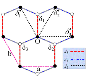
Figure 1: (Color online) Honeycomb lattice with basis vectors $\bf\delta_{0}=0$ and $\bf\delta_{1}=\frac{a}{\sqrt{3}}{\hat{j}}$, and primitive vectors ${{\bf a}=a{\hat{i}}}$ and ${{\bf b}=-\frac{a}{2}{\hat{i}}+\frac{\sqrt{3}a}{2}{\hat{j}}}$. Black and white circles indicate A and B sublattices, respectively. $\delta_{1}$, $\delta_{2}$ and $\delta_{3}$ denote the nearest neighbors and $\delta_{1}^{\prime}$, $\delta_{2}^{\prime}$ and $\delta_{3}^{\prime}$ represent the next nearest neighbors.

Now, we give a brief introduction to the formalism of MSW theory in a bipartite lattice, and then apply it to the Hamiltonian (1). MSW was introduced by Takahashi Takahashi and its basic assumption is that the ground state of spin Hamiltonian in the classical limit ($S\rightarrow\infty$), is long-range ordered. It has been shown that minimum energy condition for the classical $J_{1}-J_{2}$ Heisenberg model, gives rise to planar states katsura ; fouet . Hence, the translational invariance requires that the ordered ground state is characterized by a planar wave-vector ${\bf Q}$. Under this assumption, it is convenient to rotate the coordinate axes $(x,y,z)$ locally to ($\eta_{i}$, $\zeta_{i}$, $\xi_{i}$) at each site $i$, in such a way that $\zeta_{i}$ represents the local symmetry breaking axis. For this purpose, we introduce the following spin transformations for the honeycomb lattice which contains two lattice points per unit cell

$$S_{i,\gamma}^{x}= - \sin\left({\bf Q}\cdot{\bf r}_{i}+(\gamma-1)\phi)\right)S_{i,\gamma}^{\eta}$$

$$+ \cos\left({\bf Q}\cdot{\bf r}_{i}+(\gamma-1)\phi)\right)S_{i,\gamma}^{\zeta}$$

$$S_{i,\gamma}^{y}= \cos\left({\bf Q}\cdot{\bf r}_{i}+(\gamma-1)\phi)\right)S_{i,\gamma}^{\eta}$$

$$+ \sin\left({\bf Q}\cdot{\bf r}_{i}+(\gamma-1)\phi)\right)S_{i,\gamma}^{\zeta}$$

$$S_{i,\gamma}^{z}= - S_{i,\gamma}^{\xi},$$ (3)

where ${\bf r}_{i}$ denotes the position of each spin, $\gamma=1,2$ refers to the two lattice points (A, B sublattices) in the unit cell identified by the vectors $\delta_{0}=0$ and $\delta_{1}=\frac{a}{\sqrt{3}}{\hat{j}}$ ( see Fig. 1) and the angle $\phi$ denotes the relative rotation of the symmetry breaking axes within a unit cell. Unlike ordinary spin-wave theory, we do not make any assumption on the ordering vector ${\bf Q}$ which may differ from the classical ordering wave vector.

Applying the transformations (3) to the Hamiltonian (1), we find

$$H ={\frac{1}{2}} \sum_{nn}J_{ij}\left[({S}_{i,1}^{\eta}S_{j,2}^{\eta}+S_{i,1}^{\zeta}S_{j,2}^{\zeta})\cos[{\bf Q}\cdot({\bf r}_{i}-{\bf r}_{j})+\phi]+(-S_{i,1}^{\eta}S_{j,2}^{\zeta}+S_{i,1}^{\zeta}S_{j,2}^{\eta})\sin[{\bf Q}\cdot({\bf r}_{i}-{\bf r}_{j}+\phi]+S_{i,1}^{\xi}S_{j,2}^{\xi}\right]$$ (4)

$$+ {\frac{J_{2}}{2}}\sum_{nnn}\sum_{\gamma=1}^{2}\left[(S_{i,\gamma}^{\eta}S_{j,\gamma}^{\eta}+S_{i,\gamma}^{\zeta}S_{j,\gamma}^{\zeta})\cos[{\bf Q}\cdot({\bf r}_{i}-{\bf r}_{j})]+(-S_{i,\gamma}^{\eta}S_{j,\gamma}^{\zeta}+S_{i,\gamma}^{\zeta}S_{j,\gamma}^{\eta})\sin[{\bf Q}(\cdot{\bf r}_{i}-{\bf r}_{j})]+S_{i,\gamma}^{\xi}S_{j,\gamma}^{\xi}\right].$$

We use Dyson-Maleev (DM) transformations to obtain a bosonic representation of the spin Hamiltonian. For a bipartite lattice, like the honeycomb lattice, DM transformations are given by

$$\begin{split}S_{i,1}^{-}=\frac{1}{\sqrt{2S}}(2S-a_{i}^{\dagger}a_{i})a_{i},\ \ \ &S_{i,2}^{-}=\frac{1}{\sqrt{2S}}(2S-b_{i}^{\dagger}b_{i})b_{i},\\ S_{i,1}^{+}=\sqrt{2S}a_{i}^{\dagger},\ \ \ \ \ \ \ \ \ \ \ \ \ \ \ \ \ \ &S_{i,2}^{+}=\sqrt{2S}b_{i}^{\dagger},\\ S_{i,1}^{\zeta}=S-a_{i}^{\dagger}a_{i},\ \ \ \ \ \ \ \ \ \ \ \ \ \ \ \ &S_{i,2}^{\zeta}=S-b_{i}^{\dagger}b_{i},\end{split}$$ (5)

in which $a,b$ represent the bosonic operators in A and B sublattices, respectively, and $S$ is the value of the spins. In the above transformations the quantization axes are taken to be the local $\zeta$ axes and $S_{i}^{\pm}\equiv S_{i}^{\eta}\pm iS_{i}^{\xi}$. The commutation relations $[S_{i}^{\alpha},S_{j}^{\beta}]=i\epsilon_{\alpha\beta\gamma}S_{i}^{\gamma}\delta_{ij}$ are satisfied by the bosonic algebra between $a$ and $b$ operators, i.e, $[a_{i},a_{i^{\prime}}^{\dagger}]=\delta_{ii^{\prime}}$, $[b_{j},b_{j^{\prime}}^{\dagger}]=\delta_{jj^{\prime}},[a_{i},a_{i^{\prime}}]=[b_{i},b_{i^{\prime}}]=[a_{i},b_{i^{\prime}}]=0$. Substituting the transformations (5) into the Hamiltonian (3), one finds the following bosonic Hamiltonian

$$\begin{split}H=&\frac{1}{4}\sum_{nn}J_{ij}\{[2S(a_{i}^{\dagger}b_{j}+a_{i}b_{j}^{\dagger})-a_{i}^{\dagger}b_{j}^{\dagger}b_{j}b_{j}-a_{i}^{\dagger}a_{i}a_{i}b_{j}^{\dagger}](1+\cos({\bf Q}\cdot{\bf r}_{ij}+\phi))\\ &+[-2S(a_{i}^{\dagger}b_{j}^{\dagger}+a_{i}b_{j})+a_{i}b_{j}^{\dagger}b_{j}b_{j}+a_{i}^{\dagger}a_{i}a_{i}b_{j}](1-\cos({\bf Q}\cdot{\bf r}_{ij}+\phi))\\ &+4[S^{2}-S(a_{i}^{\dagger}a_{i}+b_{j}^{\dagger}b_{j})+a_{i}^{\dagger}a_{i}b_{j}^{\dagger}b_{j}]\cos({\bf Q}\cdot{\bf r}_{ij}+\phi)\}\\ &+\frac{J_{2}}{4}\sum_{nnn}[2S(a_{i}^{\dagger}a_{j}+a_{i}a_{j}^{\dagger})-a_{i}^{\dagger}a_{j}^{\dagger}a_{j}a_{j}-a_{i}^{\dagger}a_{i}a_{i}a_{j}^{\dagger}](1+\cos({\bf Q}\cdot{\bf r}_{ij}))\\ &+[-2S(a_{i}^{\dagger}a_{j}^{\dagger}+a_{i}a_{j})+a_{i}a_{j}^{\dagger}a_{j}a_{j}+a_{i}^{\dagger}a_{i}a_{i}a_{j}](1-\cos({\bf Q}\cdot{\bf r}_{ij}))\\ &+4[S^{2}-S(a_{i}^{\dagger}a_{i}+a_{j}^{\dagger}a_{j})+a_{i}^{\dagger}a_{i}a_{j}^{\dagger}a_{j}]\cos({\bf Q}\cdot{\bf r}_{ij})\\ &+\frac{J_{2}}{4}\sum_{nnn}[2S(b_{i}^{\dagger}b_{j}+b_{i}b_{j}^{\dagger})-b_{i}^{\dagger}b_{j}^{\dagger}b_{j}b_{j}-b_{i}^{\dagger}b_{i}b_{i}b_{j}^{\dagger}](1+\cos({\bf Q}\cdot{\bf r}_{ij}))\\ &+[-2S(b_{i}^{\dagger}b_{j}^{\dagger}+b_{i}b_{j})+b_{i}b_{j}^{\dagger}b_{j}b_{j}+b_{i}^{\dagger}b_{i}b_{i}b_{j}](1-\cos({\bf Q}\cdot{\bf r}_{ij}))\\ &+4[S^{2}-S(b_{i}^{\dagger}b_{i}+b_{j}^{\dagger}b_{j})+b_{i}^{\dagger}b_{i}b_{j}^{\dagger}b_{j}]\cos({\bf Q}\cdot{\bf r}_{ij}),\end{split}$$ (6)

where ${\bf r}_{ij}={\bf r}_{i}-{\bf r}_{j}$ is equal to $\delta_{1},\delta_{2},\delta_{3}$ for the nearest neighbors and $\pm\delta^{\prime}_{1},\pm\delta^{\prime}_{2},\pm\delta^{\prime}_{3}$ for the next to nearest neighbors (Fig. 1). Now, we use mean field theory to find an expression for the expectation value of the Hamiltonian (6), i.e. $E=\langle H\rangle$. For this purpose, we use the Wick’s theorem to calculate the expectation value of the quartic terms, hence we find

$$\begin{split}E=&-\frac{N}{2}\sum_{\delta}J(\delta)\{[S+\frac{1}{2}-f(0)+g({\delta})]^{2}(1-\cos({\bf{Q}}\cdot{{\delta}}+\phi))-[S+\frac{1}{2}-f(0)+f({\delta})]^{2}(1+\cos(\bf{Q}\cdot\delta+\phi))\}\\ &-\frac{J_{2}}{2}\sum_{\delta^{\prime}}\{[S+\frac{1}{2}-f(0)+g(\delta^{\prime})]^{2}(1-\cos({\bf{Q}}\cdot{\delta^{\prime}}))-[S+\frac{N}{2}-f(0)+f(\delta^{\prime})]^{2}(1+\cos({\bf{Q}}\cdot{\delta^{\prime}}))\},\end{split}$$ (7)

in which $\delta$ and $\delta^{\prime}$ denote the first and second neighbors, respectively, $J(\delta_{1})=J_{1}$, $J(\delta_{2})=J(\delta_{3})=J^{\prime}_{1}$ and $N$ is the number of sites. Functions $f$ and $g$ denote the expectation value of hopping and pairing of DM bosons defined as

$$\begin{split}\langle a_{i}^{\dagger}b_{j}\rangle=&\langle a_{i}b_{j}^{\dagger}\rangle\equiv f(\delta),\ \langle a_{i}^{\dagger}a_{j}\rangle=\langle b_{i}^{\dagger}b_{j}\rangle\equiv f(\delta^{\prime})-\frac{1}{2}\delta_{ij},\\ \langle a_{i}^{\dagger}a_{j}^{\dagger}\rangle=&\langle a_{i}a_{j}\rangle\equiv g(\delta^{\prime}),\ \langle b_{i}^{\dagger}b_{j}^{\dagger}\rangle=\langle b_{i}b_{j}\rangle\equiv g(\delta^{\prime}),\\ \langle a_{i}^{\dagger}b_{j}^{\dagger}\rangle=&\langle a_{i}b_{j}\rangle\equiv g(\delta),\end{split}$$ (8)

with $f(0)=f({\delta=0})$.

Then using equations (7) and (8), one finds the following expression for the ground state energy per site, $E_{0}=E/N$, in mean field approximation

$$E_{0}=\epsilon_{0}+\epsilon_{1}\cos(\phi)$$

$$+\epsilon^{\prime}_{1}[\cos(\frac{Q_{x}}{2}+\frac{\sqrt{3}Q_{y}}{2}+\phi)+\cos(-\frac{Q_{x}}{2}+\frac{\sqrt{3}Q_{y}}{2}+\phi)]$$

$$+\epsilon_{2}[\cos(Q_{x})+\cos(\frac{Q_{x}}{2}+\frac{\sqrt{3}Q_{y}}{2})+\cos(-\frac{Q_{x}}{2}+\frac{\sqrt{3}Q_{y}}{2})],$$

(9)

where

$$\epsilon_{0} = {\sum_{\delta}\frac{J(\delta)}{2}(f(\delta)^{2}-g(\delta)^{2})}$$

$$+ {\frac{J_{2}}{2}\sum_{\delta^{\prime}}(f(\delta^{\prime})^{2}-g(\delta^{\prime})^{2})},$$

$$\epsilon_{1} = \frac{J_{1}}{2}(f(\delta_{1})^{2}+g(\delta_{1})^{2}),$$

$$\epsilon^{\prime}_{1} = {\frac{J^{\prime}_{1}}{4}\sum_{i=2}^{3}(f(\delta_{i})^{2}+g(\delta_{i})^{2})},$$

$$\epsilon_{2} = {\frac{J_{2}}{12}\sum_{\delta^{\prime}}(f(\delta^{\prime})^{2}+g(\delta^{\prime})^{2})}.$$ (10)

First step in MSW procedure is to minimize the energy (9) with respect to the ordering vector $\bf{Q}$. This incorporates the competition between states with LRO at different ordering vectors $\bf{Q}$ which may not necessary be stable at the classical level Ting . Next step is to minimize $E_{0}$ with respect to $f_{ij}$ and $g_{ij}$. In the absence of external field, this minimization is done under the constraint that the expectation value of spins along the local quantization axes vanishes. The constraint, $\langle S_{i}^{\zeta}\rangle=0$, introduced by Takahashi Takahashi , to keep the number of DM bosons per site less than $2S$ ($n<2S$).

$$\langle S_{i}^{\zeta}\rangle = -S+\langle a_{i}^{\dagger}a_{i}\rangle=-S+\langle b_{i}^{\dagger}b_{i}\rangle$$ (11)

$$= -S-\frac{1}{2}+f(0)=0.$$

The Takahashi’s constraint reduces the Hilbert space dimension available to the DM bosons by reducing their average density to $S$. In a bipartite lattice, one can in fact show a significant reduction of the Hilbert space dimension from $2^{N}$ to $\frac{4}{\pi}\frac{2^{N}}{N}$ for $S=1/2$ dotsen .

For a given ordering wave vector ${\bf Q}$ and rotation $\phi$, an appropriate set of Bogoliubov transformations are defined, in terms of which the Hamiltonian equation (6) can be diagonalized in mean field approximation. Moreover, the quantities $f$ and $g$ defined by equation (8) can be parameterized in terms of the coefficients of the Bogoliubov transformations, allowing us to minimize the total energy with respect to these coefficients, under the Takahashi’s constraint (11). To satisfy the Takahashi’s constraint we need to introduce a Lagrange multiplier $\mu$ which plays the role of chemical potential for the DM bosons. In bosonic language, a magnetically ordered state can be translated to a Bose-Einstein condensate (BEC), for which $\mu=0$ cirac . For the magnetic disordered states the spontaneous magnetization is zero, hence there is no reason for vanishing of the chemical potential. In this case $\mu$ has to be calculated self-consistently to give the gap of the magnon dispersion. MSW gives a set of self-consistent equations for $g$ and $f$, whose outputs are the ground state energy, magnon energy spectrum, magnetization and spin-spin correlations. The details of this procedure are given in Appendices A and B. In the next section we apply MSW theory to the symmetric $J_{1}-J_{2}$ model.

III MSW phase diagram of symmetric $J_{1}-J_{2}$ model

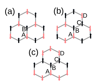
Figure 2: (Color online) Schematic representation of (a) Néel.I spin configuration comprised of two magnetic sublattices A and B, (b) Néel.II and (c) Néel.III states consisting of four magnetic sublattices A, B, C and D.

For the symmetric model $J_{1}=J^{\prime}_{1}$, minimizing the total energy (9) with respect to $Q_{x}$, $Q_{y}$ and $\phi$, gives rise to numerous commensurate and incommensurate solutions. The commensurate minima are achieved by a two-sublattice collinear ordering, given by ${\bf Q}=(0,0)$; $\phi=\pi$ (Néel.I), and two types of four-sublattices collinear ordering with ${\bf Q}=(\pi,\frac{\pi}{\sqrt{3}})$; $\phi=\pi$ (Néel.II) and ${\bf Q}=(0,\frac{2\pi}{\sqrt{3}})$; $\phi=0$ (Néel.III). The schematic spin configurations in these states are illustrated in figure 2. The incommensurate solutions are given by the spiral states ${\bf Q}=(2\cos^{-1}(\pm\frac{1}{2}\frac{3\epsilon_{1}\pm\epsilon_{2}}{\epsilon_{2}}),0\ {\rm or}\ \frac{2\pi}{3})$; $\phi=0\ {\rm or}\ \pi$ , and ${\bf Q}=(0,\frac{2}{\sqrt{3}}(\sin^{-1}(\frac{1}{2}\sin(\phi))-\phi)$ ; $\phi=\cos^{-1}(\frac{\epsilon_{2}}{\epsilon_{1}}-\frac{3\epsilon_{1}}{4\epsilon_{2}})+\pi$, where $\epsilon_{1}$ and $\epsilon_{2}$ are given by equation (10).

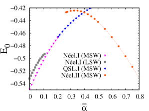
Figure 3: (Color online) Ground state energy per site (in unites of $J_{1}$) of symmetric $J_{1}-J_{2}$ model versus the frustration parameter ${\bar{\alpha}}$ for $S=1/2$. The ground state is Néel.I ordered for $0.0\leq{\bar{\alpha}}\lesssim 0.207$ (pink triangles) , quantum spin liquid with Néel.I type symmetry (QSL.I) for $0.207\lesssim{\bar{\alpha}}\lesssim 0.396$ (blue rhomboids) and Néel.II ordered for $0.396\lesssim{\bar{\alpha}}\leq 1.0$ (red diamonds). The grey squares show the ground state energies per site, obtained in linear spin wave (LSW) approximation in the Néel.I phase.

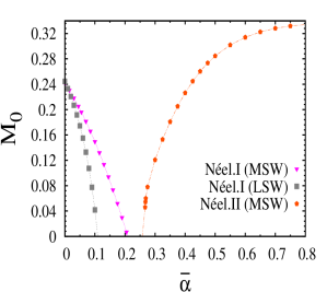
Figure 4: (Color online) Spontaneous magnetization ($M_{0}$) per site of symmetric $J_{1}-J_{2}$ model versus the frustration parameter ${\bar{\alpha}}$ for $S=1/2$. The pink triangles and red diamonds show the magnetization obtained from MSW in Néel.I and Néel.II phases, respectively. The grey squares represent the magnetization in LSW approximation.

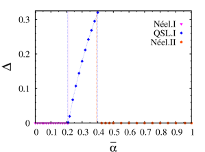
Figure 5: (Color online) Energy gap of magnon spectrum ($\Delta$) (in units of $J_{1}$) versus the frustration parameter ${\bar{\alpha}}$. $\Delta$ is zero in the Néel.I ordered phase and then grows continuously in QSL.I phase and finally drops to zero in the Néel.II ordered phase.

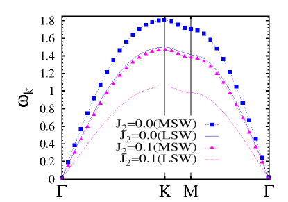
(a)  Néel.I phase

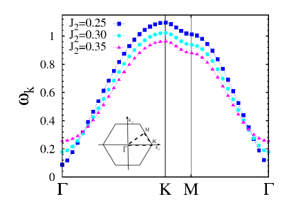
(b)  QSL phase

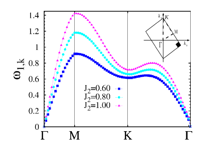
(c)  Néel.II phase

Figure 6: (Color online) Magnon energy dispersion $\omega_{k}$ (in units of $J_{1}$) along symmetry directions in the magnetic first Brillouin zone (1BZ) for (a) Néel.I, (b) QSL, and (c) Néel.II phases. The insets illustrate the magnetic 1BZ corresponding to each phase. The magnetic 1BZ of Néel.I state is the same as the 1BZ of the honeycomb lattice as shown by the inset of panel (b). The solid and dashed lines in the panel (a) represent the magnon dispersion obtained in LSW approximation.

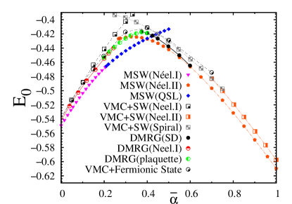
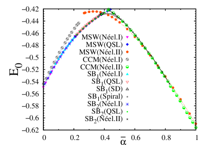
Figure 7: (Color online) Comparison of MSW results with (top) density-matrix renormalization group (DMRG)pvb7 , variational Monte Carlo (VMC) based on Jastrow and projected fermionic states (VMC+fermionic state) VMC-sondhi and spin wave states (VMC+SW state) Ciolo , and (bottom) the coupled cluster method (CCM) pvb4 and Schwinger boson approach (SB₁ SB-lamas1 and SB₂ SB-china . SD denotes staggered dimerized state.

Having a long range ordered (LRO) ground state, requires the gapless excitation spectrum as the result of Goldstone theorem. This condition leads to vanishing of the chemical potential $\mu$ (defined by Eq. (17)), in the ordered state as a requirement of BEC transition cirac . To calculate the energy and magnetization for each type of ordering one needs to solve the self-consistent equations (18), (19), (20), (21) and (22), with $\mu=0$. After convergence, these equations give the spontaneous magnetization $M_{0}$ and the functions $f_{ij}$ and $g_{ij}$, then substitution of $f_{ij}$ and $g_{ij}$ in equation (7) gives the ground state energy per site $E_{0}$. The magnon excitation spectrum is given by equation (23), and spin-spin correlations can be calculated by the equations (24) and (25). For Néel.II and III orderings, it is more convenient to use a four-sublattice unite cell (Fig.2-b,c), wherefore the ordering wave vector is $Q=0$. Using the larger unit cell in real space leads to reduction of the size of magnetic Brillouin zone in ${\bf K}$-space and so the number of singular points, hence making the convergence of corresponding self-consistent equations much easier (see Appendix B for details). In this case, the physical quantities of interest can be calculated by solving the set of equations (30).

Following the above procedure, MSW results that within the possible ordered state, The Néel.I and Néel.II acquire the minimum energy for $0\leq{\bar{\alpha}}\lesssim 0.207$ and ${\bar{\alpha}}\gtrsim 0.25$, respectively. The dependence of ground state energy per site ($E_{0}$) and corresponding spontaneous magnetization ($M_{0}$) on the frustration parameter ${\bar{\alpha}}$ are illustrated in figures 3 and 4, respectively. In figures 3 and 4, $E_{0}$ and $M_{0}$ obtained by the linear spin wave (LSW) theory, are also represented for Néel.I state. LSW indicates that the Néel.I phase is stable only to ${\bar{\alpha}}\approx 0.11$. Therefore, a comparison between LSW and MSW shows that the the nonlinear interactions, taken into account by MSW in mean field approximation, lower the energy of the Néel.I phase and also increases its stability against the frustration up to ${\bar{\alpha}}\approx 0.207$.

On the other hand, for ${\bar{\alpha}>0.25}$ we found that Néel.II has lower energy with respect to the Néel.III and also the spiral states. The energy per site and magnetization, corresponding to this type of ordering, is plotted for the range ${0.25<\bar{\alpha}\leq 0.8}$ in figures 3 and 4. It is important to mention that Néel.II state is not a classically stable state. Indeed assuming such an ordering and using LSW approximation, it is found that complex numbers appear in its spin excitation spectrum which makes this state unstable. Hence, the stability of this phase in MSW can be attributed to the nonlinear magnon-magnon interactions.

For the interval ${0.207\lesssim\bar{\alpha}\lesssim 0.25}$, however, no ordered state is found to be stable. Indeed, the magnetization of Néel.I state falls continuously to zero at ${\bar{\alpha}\approx 0.207}$, above which no stable solution of self-consistent equations corresponding to Néel.I ordering is possible with the BEC condition $\mu=0$. However, starting from Néel.I state and relaxing the BEC condition and setting $M_{0}=0$, it is possible to obtain from MSW equations a magnetically disordered state with finite chemical potential and vanishing magnetization for ${\bar{\alpha}}\gtrsim 0.207$. In this case the chemical potential, $\mu$, has to be considered as a quantity which is to be found self-consistently.

In addition to the $SU(2)$ symmetry of the spin Hamiltonian (1), such a disordered phase preserves all the symmetries of the lattice, i.e. the $C_{3}$ and $C_{6}$ rotational and translational symmetries. In fact all the attempts to find a solution with broken rotational symmetry, for example a solution with not equal pairing and hopping functions on different bonds, were unsuccessful. Such a magnetically disordered state which respects all the symmetries of the Hamiltonian and the lattice is called quantum spin liquid (QSL) state. As it can be seen from the figure 3, the energy curve of the Néel.I state connects smoothly to the QSL state, an indication of a continuous phase transition between these two ground states. Moreover the calculation of spin gap, illustrated in figure 5, shows the continuous rise of the magnon gap in this phase. Interestingly, the stability of QSL state goes beyond ${\bar{\alpha}=0.25}$ and its energy is lower than the Néel.II phase up to ${\bar{\alpha}}\approx 0.397$ where it crosses the energy curve of Néel.II. As a conclusion, the transition between these two phases are first order. Figure 5 shows that at this transition point the spin gap drops discontinuously to zero.

Since these gapped QSL phase is obtained by starting from the Néel.I state it possess all the symmetries of Néel.I, hence we call it QSL.I. Starting from Néel.II and III, it is also possible to find QSL states, however with higher energy with respect to QSL.I. Calculation of spin-spin correlations for QSL.I shows the existence short-range Néel.I type correlations in this phase (see Table.1 and figure 9-b).

Figure 6, represents the magnon dispersion along the symmetry directions in the magnetic Brillouin Zone of for Néel.I (panel-(a)), QSL (panel-(b)) and Néel.II (panel-(c)) phases. In panel-(a), the LSW magnon dispersion is also shown to have lower energy with respect to the MSW dispersion, indicating the more rigidity of ordered phase as a result of magnon-magnon interaction. In panel-(c) of figure 6 only the lower branch of magnon dispersion, given by equation (31), is plotted.

To close this section, we compare the MSW results with some other methods. Figure 7 displays such a comparison, in top panel of this figure the MSW ground state energies are co-platted with similar results obtained by density-matrix renormalization group (DMRG) pvb7 , variational Monte Carlo (VMC) approaches based on projected fermionic states (VMC+fermionic state) VMC-sondhi , VMC based on spin wave states (VMC+SW state) Ciolo . The comparison of MSW results with CCM pvb4 and Schwinger boson (SB) mean field approaches SB₁ SB-lamas1 and SB₂SB-china is also illustrated in the bottom panel of this figure.

The top panel clearly shows that the MSW ground state energies in the three phases lay below the energies obtained by DMRG and VMC. Specifically, for the disordered region the QSL state proposed by MSW has lower energy with respect to the plaquette valence bond (PVB) and also staggered dimerized (SD) (both proposed by DMRG). For ${\bar{\alpha}\gtrsim 0.4}$, the Néel.II state obtained by MSW has lower energy than the spiral state proposed by VMC+SW Ciolo . VMC base upon fermionic states yields a Néel.I phase for $0\leq{\bar{\alpha}}\lesssim 0.08$, a $Z_{2}$ QSL state for $0.08\lesssim{\bar{\alpha}}\lesssim 0.3$ and a SD state for ${\bar{\alpha}}\gtrsim 0.3$ VMC-sondhi

On the other hand, The bottom panel shows that MSW results are in a very good agreement with Schwinger boson (SB) mean filed approach SB-lamas1 ; SB-china in the Néel.I and QSL phases, while it gives lower energy for this phase with respect to CCM pvb4 . For the Néel.II state, although the MSW result agrees well with SB₂ and CCM for ${\bar{\alpha}}\gtrsim 0.6$, nevertheless its energy lays below the ones obtained by other two for ${\bar{\alpha}}\lesssim 0.6$. Hence, the transition point from QSL to Néel.II which is ${\bar{\alpha}\approx 0.42}$ for SB₂, moved to a smaller value ${\bar{\alpha}\approx 0.396}$ for MSW. Moreover, by calculation of PVB and SD susceptibilities, CCM predicts a PVB state for $0.207<{\bar{\alpha}}<0.385$ and SD ground states for $0.385<{\bar{\alpha}}<0.65$. SB₁ SB-lamas1 also results in a SD ordering for $0.373\lesssim{\bar{\alpha}}\lesssim 0.398$ with a competitive energy with the QSL.I found by MSW. SB₁ also gives rise to a spiral ground state for $0.398<{\bar{\alpha}}<0.5$ with a larger energy than the Néel.II obtained by MSW.

Like MSW, the entangled pair variational ansatz (not shown in Fig.7) eps yields a Néel.I ordered state for $0\leq{\bar{\alpha}}\lesssim 0.2$, a Néel.II state for $0.4\lesssim{\bar{\alpha}}<1$ and a symmetry preserving disordered state for $0.2\lesssim{\bar{\alpha}}\lesssim 0.4$, though with higher energies respect to MSW.

IV phase diagram of distorted model

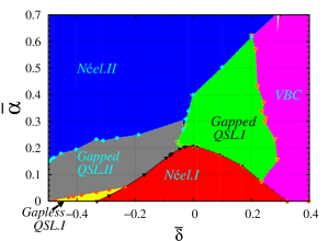
Figure 8: (Color online) MSW phase diagram of $S=1/2$ distorted $J_{1}-J_{2}$ honeycomb anti-ferromagnet. QSL.I and II denotes the quantum spin liquid states originating from Néel.I and Néel.II, respectively. VBC stands for valence bond crystal state.

In this section we discuss the phase diagram of $S=1/2$ distorted model Hamiltonian (1). The MSW phase diagram of the model is represented in figure 8 in plane of the distortion parameter ${\bar{\delta}}$ and frustration ${\bar{\alpha}}$. Like the symmetric model, magnetically ordered phase in the presence of distortion are found to be the collinear states Néel.I and II.

Figure 8, shows that the maximum stability of Néel.I state occurs for isotropic model $\bar{\delta}=0$. Distortion in both c positive ($\bar{\delta}>0$ i.e. $J_{1}>J^{\prime}_{1}$) and negative ($\bar{\delta}<0$ i.e. $J_{1}<J^{\prime}_{1}$) cases, makes this phase more fragile against frustration. For $|\bar{\delta}|\approx 0.3$, Néel.I phase becomes totally unstable for any $\bar{\alpha}>0$. The stability region of Néel.I state versus distortion is in agreement with the results of renormalization group (RG) calculations done on the nonlinear sigma model (NLSM) presentation of the model takano . However, the RG-NSLM underestimates the stability range of this phase against frustration, i.e. finds the maximum stability range $0\leq{\bar{\alpha}\lesssim 0.11}$ for the symmetric model (${\bar{\delta}=0}$).

For Néel.II phase, while the positive distortion ($\bar{\alpha}>0$) has a destructive effect on the stability of this phase against the frustration, nevertheless, negative distortion ($\bar{\delta}<0$) extends its stability to lower value of frustration. Note that in order to make $J_{1}$ and $J^{\prime}_{1}$ positive, the distortion parameter should be in the interval $[-0.5,1.0]$.

In addition to these to ordered disordered phases we find four magnetically distinct disordered phases, (i) a valence bond crystal (VBC) phase for large positive distortion, (ii) a gapped QSL originating form the Néel.I state (gapped QSL.I) for intermediate positive and small negative distortions, (iii) a gapped QSL originating from the Néel.II state(gapped QSL.II) for negative distortions and intermediate frustration and (iv) gapless QSL originating from Néel.I (gapless QSL.I) for large negative distortion and small frustration. Apart from the gapped QSl.II, all the other three disordered phase VBC, gapped and gapless QSL.I are the self-consistent solutions of MSW equations with started from the Néel.I ordering state, but with vanishing spontaneous magnetization. On the other hand, in the stability region of gapped QSl.II, starting from Néel.I ordering, the self-consistent equations does not converge to any stable solution. However, in this region assuming a Néel.II type ordering, a stable disordered state comes out of MSW equations.

To gain insight into nature of the disordered states, we calculated the spin-spin correlation for the nearest and next to nearest neighbor spins. The correlation data are given in Table.1 for a representative point in each phase. These results are also displayed schematically in figure 9.

As it is clear from the first three rows of Table.1 and panels (a),(b) and (c) of figure 9, in QSL.I there are short-range correlation inherited from Néel.I ordering, i.e. nearest neighbor negative (AF) and next to nearest neighbor positive (F) correlations. In absence of distortion ($\bar{\delta}=0$) the correlations are the same in all directions. However, in the presence of distortion, the AF correlations are stronger for the nearest neighbor bonds with larger exchange coupling (figure 9-(a) and (c)).

While for positive and small negative distortion the QSL.I state is gapped, for small frustration and large negative distortions (say $-0.5\leq\bar{\delta}\lesssim-0.3$) this phase is gapless. It can be seen from the first row of Table.1 that the AF correlations along $J^{\prime}$-bonds are larger than the one along $J$-bond, by two orders of magnitude, hence if $J_{2}$ is small enough, the honeycomb spin system in this case can be considered as a system of weakly coupled chains with coupling $J^{\prime}$. Therefore, the fact that ground state of a $S=1/2$ Heisenberg chain is a gapless spin liquid state, would be a justification for QSL.I state in this region being gapless.

For large positive distortions, there are vanishing correlations between the nearest neighbor correlations in $\delta_{2}$ and $\delta_{3}$ directions as well as between all the second neighbors. In this case, the spins residing on $J_{1}$-bonds ($\delta_{1}$ directions) form strong singlet valence bonds (figure 9-(d)). In such a strong dimerized state, singlets are prevented from hopping to the neighboring bonds and so are frozen. This is the reason for a calling it a valence bond crystal (VBC).

Finally, in the region of the stability for gapped QSL.II (negative distortions and moderate frustration) the AF correlation along $J_{1}$-bonds as well as the positive correlations along $\delta_{1}$ and $\delta_{2}$ correlations are negligible (the last row of Table.1 and figure 9-(e)). In this phase the system can also be considered as effectively decoupled chains with nearest negative and next to nearest positive correlations. It seems the enhanced frustrating interaction $J_{2}$ between the second neighbors pushes the two spins within each unit cell into their high spin state, hence, roughly speaking, this spin system can be effectively described by an $S=1$ chains for which spin excitations are gapped.

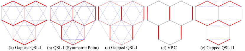
Figure 9: (Color online) Schematic representation of spin-spin correlations for the first and second neighbors for a representative pint in the phases: (a) gapless QSL.I, (b) symmetric gapped QSL.I ($\bar{\delta}=0$), (c) distorted gapped QSL. I, (e) valence bond solid (VBC) and (d) gapped QSL.II. The solid red and dotted blue lines denote negative (AF) and positive (F) correlations. The thickness of the lines are proportional to the correlation magnitude.

Table 1: Spin-spin correlation functions of nearest neighbors ( $\langle S_{\bf{i}}\cdot S_{{\bf i}+{\bf\delta}_{1}}\rangle$, $\langle S_{\bf i}\cdot S_{{\bf i}+{\bf\delta}_{2}}\rangle$, $\langle S_{\bf{i}}\cdot S_{{\bf i}+{\bf\delta}_{3}}\rangle$) and next to nearest neighbors ($\langle S_{\bf{i}}\cdot S_{{\bf i}+{\bf\delta}^{\prime}_{1}}\rangle,\langle S_{\bf i}\cdot S_{{\bf i}+{\bf\delta}^{\prime}_{2}}\rangle,\langle S_{\bf{i}}\cdot S_{{\bf i}+{\bf\delta}^{\prime}_{3}}\rangle$) in different phases of distorted honeycomb anti-ferromagnet. The vectors ${\bf\delta}_{1},{\bf\delta}_{2},{\bf\delta}_{3},{\bf\delta}^{\prime}_{1},{\bf\delta}^{\prime}_{2}$ and ${\bf\delta}^{\prime}_{3}$ are shown in Fig. 1.

${\bar{\alpha}}$	${\bar{\delta}}$	$\langle S_{\bf{i}}\cdot S_{{\bf i}+{\bf\delta}_{1}}\rangle$	$\langle S_{\bf{i}}\cdot S_{{\bf i}+\delta_{2,3}}\rangle$	$\langle S_{\bf{i}}\cdot S_{{\bf i}+\delta^{\prime}_{1,2}}\rangle$	$\langle S_{\bf{i}}\cdot S_{{\bf i}+\delta^{\prime}_{3}}\rangle$	State
$0.02$	$-0.4$	$-0.0065$	$-0.3276$	$0.0282$	$0.0282$	Gapless QSL.I
$0.25$	$0$	$-0.1720$	$-0.1720$	$0.0411$	$0.0411$	gapped QSL.I (symmetric)
$0.3125$	$0.125$	$-0.3217$	$-0.05680$	$0.0122$	$0.0122$	Gapped QSL.I
$0.425$	$0.350$	$-0.3753$	$-4.2\times 10^{-7}$	$5.0\times 10^{-8}$	$5.0\times 10^{-8}$	VBC
$0.1875$	$-0.125$	$3\times 10^{-11}$	$-0.2230$	$-4.3\times 10^{-9}$	$0.0615$	Gapped QSL.II

V conclusion

Taking advantage of DM transformation, which are exact and hence unlike Holstein-Primakoff transformation need not be truncated, MSW provides a powerful tool to extract the phase diagram of spin systems. Using MSW, we explored the ground state of symmetric and distorted $S=1/2$ Heisenberg $J_{1}-J_{2}$ antiferromagnet in honeycomb lattice. For the symmetric model, where all equivalent bonds in honeycomb lattice have equal exchange couplings, we found two types of collinear ordering in small and large frustration limit, namely a two-sublattice ordering Néel.I for $0\leq J_{2}/J_{1}\lesssim 0.207$ and a four-sublattice ordering Néel.II for $J_{2}/J_{1}\gtrsim 0.396$. The Néel.II is not a classical solution and so is unstable when quantum fluctuations are taken into account by linear spin wave theory. Indeed, for $S=1/2$ the enhanced nonlinear quantum fluctuations tend to stabilize this phase. For intermediate frustration $0.207\lesssim J2/J1\lesssim 0.396$ a magnetically disordered state which preserves all the symmetries of the system is found to be the ground state that is a gapped QSL. The short-range correlations in this QSL has the symmetries of Néel.I, then we coined the name QSL.I for this phase. We found that these two phases transform to each other by a continuous phase transition. However, symmetries of the QSL.I are different from Néel.II, and so a first order transition is found between these two states as expected. As a conclusion the order-disorder transitions in this system can be described in the framework of Landau-Ginzburg theory.

Introducing the distortion to the model breaks its $C_{3}$ symmetry. This leads to the emergence of new phases as the result of the interplay between distortion and frustration. These new phases, all being magnetically disordered, are a gapless QSL.I originating from Néel.I ordering, a gapped QSL.II originating from Néel.II and a valence bond solid state where the singlet dimers are frozen on the bonds with larger coupling. We discussed that in both gapless QSL.I and gapped QSL.II phases, the model can be effectively be described in terms of weakly coupled zigzag chains.

The main privilege of MSW over other methods, such as DMRG, VMC and ED, is that it is free from finite size effect. However, validity of the mean-filed approximation incorporated in this method might be under question when the quantum fluctuations become large. The quantum fluctuations are significantly large in the disordered states where the spontaneous magnetization, or in terms of bosons the condensate, vanishes. This suggest that the QSL states proposed for the disordered region of the phase diagram has to be considered cautiously. Therefore, to improve the validity of MSW states, one could consider them as the initial wave function for the variational methods.

Appendix A Derivation of MSW self-Consistent equations

To diagonalize the Hamiltonian (6) in mean field approximation, we need to define the Bogoliubov transformations

$$\alpha_{\bf k} = \cosh(\theta_{\bf k})a_{\bf k}-\sinh(\theta_{\bf k})b_{-{\bf k}}^{\dagger},$$

$$\beta_{-\bf k}^{\dagger} = -\sinh(\theta_{\bf k})a_{\bf k}+\cosh(\theta_{\bf k})b_{-{\bf k}}^{\dagger},$$

where $a_{\bf k}$ and $b_{-\bf k}^{\dagger}$ are the Fourier transformations of $a_{i}$ and $b_{j}^{\dagger}$ (defined by equation (5)),

$$a_{\bf k} = \sqrt{\frac{2}{N}}\sum_{i\in A}e^{-\bf{ik}\cdot{\bf r}_{i}}a_{i},$$

$$b_{-\bf k}^{\dagger} = \sqrt{\frac{2}{N}}\sum_{j\in B}e^{-\bf{ik}\cdot{\bf r}_{j}}b_{j}^{\dagger},$$

in which $N$ is the total number of sites. The mean field Hamiltonian in its diagonalized form, in terms of noninteracting Bogoliubov quasiparticles, is written as

$$\begin{split}&H_{\rm MF}=\sum_{\bf k}[\omega_{\bf k}(\alpha_{\bf k}^{\dagger}\alpha_{\bf k}+\beta_{\bf k}^{\dagger}\beta_{\bf k})]+NE_{0},\end{split}$$ (14)

where $\omega_{k}$ is the excitation energy spectrum and $E_{0}$ is the ground state energy per site given by equation (9). Substituting $a_{i}$ and $b_{i}$ in equation (8) in terms of Bogolon operators (LABEL:BogoN), for a pair of DM bosons at a given displacement vector ${\bf r}_{ij}={\bf r}_{i}-{\bf r}_{j}$, one finds for hopping ( $f_{ij}=f({\bf r}_{ij})$) and pairing ($g_{ij}=g({\bf r}_{ij})$) expectation functions

$$f_{ij}=\frac{1}{N}\sum_{\bf k}^{\prime}\cosh(2\theta_{\bf k})\exp(-{\bf ik}\cdot{\bf r}_{ij}),$$ (15)

with $\ i,j\in A$ or $B$, and

$$g_{ij}=\frac{1}{N}\sum_{\bf k}^{\prime}\sinh(2\theta_{\bf k})\exp(-{\bf ik}\cdot{\bf r}_{ij}),$$ (16)

with $i\in A$ and $j\in B$. Otherwise $f_{ij}$ and $g_{ij}$ vanish. In equation (15) and (16), $\sum_{\bf k}^{\prime}$ denotes the sum of over half of the Brillouin zone.

We then minimize the mean filed energy (7) with respect to $\theta_{k}$, under the constraint (11), that is

$$\frac{\partial[E-\mu f(0)]}{\partial\theta_{\bf k}}=0,\\$$ (17)

where the Lagrange multiplier $\mu$ can considered the chemical potential needed to fix the number of DM bodons in order to fulfill the Takahashi’s constraint. Minimization (17) yields the following set of self-consistent equations

$$f_{ij}=M_{0}+\frac{1}{N}\sum_{{\bf k}\neq{\bf 0}}^{\prime}\frac{B_{\bf k}}{\omega_{\bf k}}e^{\bf{ik}\cdot\bf{r}_{ij}},$$ (18)

$$g_{ij}=M_{0}+\frac{1}{N}\sum_{{\bf k}\neq{\bf 0}}^{\prime}\frac{A_{\bf k}}{\omega_{\bf k}}e^{\bf{ik}\cdot\bf{r}_{ij}},$$ (19)

and

$$M_{0}=S+\frac{1}{2}-\frac{1}{N}\sum_{\bf k\neq 0}^{\prime}\frac{B_{\bf k}}{\omega_{\bf k}}.$$ (20)

here $A_{\bf k}$ and $B_{\bf k}$ are given by

$$A_{\bf k}=\frac{1}{2}\sum_{\delta}J(\delta)g(\delta)e^{{\bf{ik}\cdot\delta}}+\frac{J_{2}}{2}\sum_{\delta^{\prime}}g(\delta^{\prime})e^{{\bf{ik}\cdot\delta^{\prime}}},$$ (21)

and

$$B_{\bf k} = \frac{1}{2}\sum_{\delta}J(\delta)[g(\delta)-f(\delta)(1-e^{{\bf{ik}\cdot\delta}})]$$ (22)

$$+ \frac{J_{2}}{2}\sum_{\delta^{\prime}}[g(\delta^{\prime})-f(\delta^{\prime})(1-e^{{\bf{ik}\cdot\delta^{\prime}}})]+\mu.$$

In equation (20), $M_{0}$ denotes the spontaneous magnetization. In terms of DM bosons, $M_{0}$ would be the order parameter of BEC transition, hence the physical meaning of $M_{0}=\langle a_{{\bf k}=0}^{\dagger}a_{\bf k=0}\rangle/N=\langle b_{\bf k=0}^{\dagger}b_{\bf k=0}\rangle/N$, is the number bosons condensed in the zero energy. Therefore, the nonzero value of condensate is an indication of existence of long-range ordering (LRO) in magnetic state of the spin system.

The magnon energy spectrum is also given by

$$\omega_{\bf k}=\sqrt{B_{\bf k}^{2}-A_{\bf k}^{2}},$$ (23)

At ${\bf k}={\bf 0}$, we have from Eqs. (21) and (22) that $B_{{\bf k=0}}=A_{{\bf k=0}}+\mu$.

For each ordering wave vector ${\bf Q}$, the spin-spin correlations function can be obtained as

$$\langle S_{i}.S_{j}\rangle =-\frac{1}{2}[(S+\frac{1}{2}-f(0)+g_{ij})^{2}(1-\cos({\bf Q}\cdot{\bf r}_{ij}+\phi))-(S+\frac{1}{2}-f(0)+f_{ij})^{2}(1+\cos({\bf Q}\cdot{\bf r}_{ij}+\phi))],$$ (24)

for $\ i\in A\ {\rm and}\ j\in B$ and

$$\langle S_{i}.S_{j}\rangle =-\frac{1}{2}[(S+\frac{1}{2}-f(0)+g_{ij})^{2}(1-\cos({\bf Q}\cdot{\bf r}_{ij}))-(S+\frac{1}{2}-f(0)+f_{ij})^{2}(1+\cos({\bf Q}\cdot{\bf r}_{ij}))],$$ (25)

for $\ i\ {\rm and}\ j\in A\ {\rm or}\ B$.

Appendix B Derivation of self-consistent equations for Néel.II and III states

For Néel.II and III states, owing to their four-sublattice magnetic pattern (Fig.2-b,c), we define the Bogoliubov transformations as

$$\alpha_{1,{\bf k}}=\frac{1}{\sqrt{2}}(\cosh({\theta^{+}_{\bf k}})a_{\bf k}-\sinh({\theta^{+}_{\bf k}})b_{-\bf k}^{\dagger}-\sinh({\theta^{+}_{\bf k}})c_{-\bf k}^{\dagger}+\cosh({\theta^{+}_{\bf k}})d_{\bf k}),$$

$$\beta_{1,-{\bf k}}^{\dagger}=\frac{1}{\sqrt{2}}(-\sinh({\theta^{+}_{\bf k}})a_{\bf k}+\cosh({\theta^{+}_{\bf k}})b_{-\bf k}^{\dagger}+\cosh({\theta^{+}_{\bf k}})c_{-\bf k}^{\dagger}-\sinh({\theta^{+}_{\bf k}})d_{\bf k}),$$

$$\alpha_{2,-\bf k}^{\dagger}=\frac{1}{\sqrt{2}}(\cosh({\theta^{-}_{\bf k}})a_{k}-\sinh({\theta^{-}_{\bf k}})b_{-\bf k}^{\dagger}+\sinh({\theta^{-}_{\bf k}})c_{-\bf k}^{\dagger}-\cosh({\theta^{-}_{\bf k}})d_{\bf k}),$$

$$\beta_{2,\bf k}=\frac{1}{\sqrt{2}}(-\sinh({\theta^{-}_{\bf k}})a_{\bf k}+\cosh({\theta^{-}_{\bf k}})b_{-\bf k}^{\dagger}-\cosh({\theta^{-}_{\bf k}})c_{-\bf k}^{\dagger}+\sinh({\theta^{-}_{\bf k}})d_{\bf k}),$$ (26)

Then following a similar approach discussed in Appendix A, after minimizing the energy with respect to $\theta_{\bf k}^{-}$ and $\theta_{\bf k}^{+}$, that is

$$\frac{\partial[E-\mu f(0)]}{\partial\theta_{\bf k}^{\pm}}=0,\\$$ (27)

and defining $A^{\pm}_{\bf k}$ and $B^{\pm}_{\bf k}$ as

$$A_{\bf k}^{\pm}=\frac{1}{2}\sum_{\delta}J(\delta)g(\delta)e^{{\bf{ik}\cdot\delta}}\pm\frac{J_{2}}{2}\sum_{\delta^{\prime}}g(\delta^{\prime})e^{{\bf{ik}\cdot\delta^{\prime}}},$$ (28)

and

$$B_{\bf k}^{\pm} = \frac{1}{2}\sum_{\delta}J(\delta)[g(\delta)-f(\delta)(1\pm e^{{\bf{ik}\cdot\delta}})]$$ (29)

$$+ \frac{J_{2}}{2}\sum_{\delta^{\prime}}[g(\delta^{\prime})-f(\delta^{\prime})(1-e^{{\bf{ik}\cdot\delta^{\prime}}})]+\mu,$$

one finds the following set of self-consistent equations

$$M_{0}=S+\frac{1}{2}-\frac{1}{2N}\sum_{{\bf k}\neq 0}^{\prime}(\frac{B_{\bf k}^{+}}{\omega_{\bf k}^{+}}+\frac{B_{\bf k}^{-}}{\omega_{\bf k}^{-}}),$$

$$f_{ij}=M_{0}+\frac{1}{2N}\sum_{{\bf k}\neq 0}^{\prime}(\frac{B_{\bf k}^{+}}{\omega_{\bf k}^{+}}-\frac{B_{\bf k}^{-}}{\omega_{\bf k}^{-}})e^{i\bf{k}\cdot\bf{r}_{ij}},\ \ {\rm for}\ (i\in A;j\in D)\ {\rm or}\ (i\in B\ ;j\in C)$$

$$f_{ij}=M_{0}+\frac{1}{2N}\sum_{{\bf k}\neq 0}^{\prime}(\frac{B_{\bf k}^{+}}{\omega_{\bf k}^{+}}+\frac{B_{\bf k}^{-}}{\omega_{\bf k}^{-}})e^{i\bf{k}\cdot\bf{r}_{ij}},\ \ {\rm for}\ i,j\in A,{\rm}B,{\rm}C,{\rm or\rm}\ D$$

$$g_{ij}=M_{0}+\frac{1}{2N}\sum_{{\bf k}\neq 0}^{\prime}(\frac{A_{\bf k}^{+}}{\omega_{\bf k}^{+}}+\frac{A_{\bf k}^{-}}{\omega_{\bf k}^{-}})e^{i\bf{k}\cdot\bf{r}_{ij}},\ \ {\rm for}\ (i\in A;j\in B)\ {\rm or}\ (i\in C\ ;j\in D)$$

$$g_{ij}=M_{0}+\frac{1}{2N}\sum_{{\bf k}\neq 0}^{\prime}(\frac{A_{\bf k}^{+}}{\omega_{\bf k}^{+}}-\frac{A_{\bf k}^{-}}{\omega_{\bf k}^{-}})e^{i\bf{k}\cdot\bf{r}_{ij}},\ \ {\rm for}\ (i\in A;j\in C)\ {\rm or}\ (i\in B\ ;j\in D)$$

$${\rm otherwise}\hskip 14.22636ptf_{ij}=g_{ij}=0.$$ (30)

Néel.II consists of four sublattices, then there are two branches of magnon excitations for this phase given by

$$\begin{split}&\omega_{1,{\bf k}}=\sqrt{{B_{\bf k}^{+}}^{2}-{A_{\bf k}^{+}}^{2}},\\ &\omega_{2,{\bf k}}=\sqrt{{B_{\bf k}^{-}}^{2}-{A_{\bf k}^{-}}^{2}}.\end{split}$$ (31)

References

- (1) V. Kataev, A. Möller, U. Löw, W. Jung, N. Schittner, M. Kriener, and A. Freimuth, J. Magn. Magn. Mater. 310, 290 (2005).
- (2) O. Smirnova, M. Azuma, N. Kumada, Y. Kusano, M. Matsuda, Y. Shimakawa, T. Takei, Y. Yonesaki, and N. Kinomura, Journal of the American Chemical Society 131, 8313 (2009).
- (3) J. H. Roudebush, N. H. Andersen, R. Ramlau, V. O. Garlea, R. Toft-Petersen, P. Norby, R. Schneider, J. N. Hay, and R. J. Cava, Inorg. Chem. 52, 6083 (2013).
- (4) M. Yehia, E. Vavilova, A. Möller, T. Taetz, U. Löw, R. Klingeler, V. Kataev, and B. Büchner, Phys. Rev. B, 81, 060414(R) (2010).
- (5) Z. Y. Meng, T. C. Lang, S. Wessel, F. F. Assaad, A. Muramatsu, Nature 464 847 (2010).
- (6) S. Sorella, Y. Otsuka, and S. Yunoki, Scientific Reports 2, 992 (2012);
- (7) F.F. Assaad, and I.F. Herbut, Phys. Rev. X 3, 031010 (2013).
- (8) B. K. Clark, arXiv:1305.0278.
- (9) S. Katsura, T. Ide, and Y. Morita, J. Stat. Phys. 42, 381 (1986).
- (10) J. D. Reger, J. A. Riera, and A. P. Young, J. Phys.: Condens. Matter 1, 1855 (1989).
- (11) T. Einarsson and H. Johannesson, Phys. Rev. B 43, 5867 (1991).
- (12) W. H. Zheng, J. Oitmaa and C. J. Hamer Phys. Rev. B 44, 10789 (1991).
- (13) J. Oitmaa, C. J. Hamer and Zheng Weihong, Phys. Rev. B 45, 9834 (1992).
- (14) J. B. Fouet, P. Sindzingre, and C. Lhuillier, Eur. Phys. J. B 20, 241 (2001).
- (15) K. Takano, Phys. Rev. B 74, 140402(R) (2006).
- (16) Z. Noorbakhsh, F. Shahbazi, S. A. Jafari, G. Baskaran, J. Phys. Soc. Jpn. 78, 054701 (2009).
- (17) S. Okumura, H. Kawamura, T. Okubo, and Y. Motome, J. Phys. Soc. Jpn. 79, 114705 (2010).
- (18) A. Mulder, R. Ganesh, L. Capriotti, and A. Paramekanti, 81, 214419 (2010).
- (19) J. Oitmaa, R. R. P. Singh, Phys. Rev. B 85, 014428 (2012).
- (20) H. Mosadeq, F. Shahbazi, and S. A. Jafari, J. Phys. Condens. Matter, 23, 226006 (2011).
- (21) A. F. Albuquerque, D. Schwandt, B. Hetenyi, S. Capponi, M. Mambirini, A. M. Lauchli, Phys. Rev. B 84, 024406 (2011).
- (22) J. Reuther, D. A. Abanin, T. Thomale, Phys. Rev. B 84, 014417 (2011).
- (23) P. H. Y. Li, R. F. Bishop, D. J. J. Farnell, and C. E. Campbell, J. Phys.: Condens. Matter 24, 236002 (2012); Phys. Rev. B 86, 144404 (2012).
- (24) R. F. Bishop, P. H. Y. Li, and C. E. Campbell, J. Phys.:Condens. Matter 25, 306002 (2013).
- (25) R. Ganesh, S. Nishimoto, and J. van den Brink, Phys. Rev. B 87, 054413 (2013).
- (26) Z. Zhu, D. A. Huse, and S. R. White, Phys. Rev. Lett. 110, 127205 (2013).
- (27) S.-S. Gong, D. N. Sheng, O. I. Motrunich, and M. P. A. Fisher, Phys. Rev. B 88, 165138 (2013).
- (28) D. C. Cabra, C. A. Lamas, and H. D. Rosales Phys. Rev. B 83, 094506 (2011).
- (29) F. Wang, Phys. Rev. B 82, 024419 (2010).
- (30) Y-M. Lu, and Y. Ran, Phys. Rev. B 84, 024420 (2011).
- (31) B. K. Clark, D. A. Abanin, and S. L. Sondhi, Phys. Rev. Lett. 107, 087204 (2011).
- (32) H. Zhang, and C. A. Lamas, Phys. Rev. B 87, 024415 (2013).
- (33) X.-L. Yu, D.-Y. Liu, P. Li, and L.-J. Zou, Physica E 59, 41 (2014)
- (34) F. Mezzacapo, and M. Boninsegni, Phys. Rev. B 85, 060402 (2012).
- (35) H-Y. Yang, A.F. Albuquerque, S. Capponi, A.M. Lauchli, K.P. Schmidt, New J. Phys. 14, 115027 (2012).
- (36) S. Pujari, K. Damle, and F. Alet, Phys. Rev. Lett 111, 087203 (2013).
- (37) M. H Zare, H. Mosadeq, F. Shahbazi and S. A. Jafari, J. Phys.: Condens. Matter 26 456004 (2014).
- (38) P. H. Y. Li, R. F. Bishop, and C. E. Campbell, Phys. Rev. B 89, 220408(R).
- (39) A. D. Ciolo, J. Carrasquilla, F. Becca, M. Rigol and V. Galitski, Phys. Rev. B 89, 094413 (2013).
- (40) S.-S. Gong, W. Zhu, and D. N. Sheng, Phys. Rev. B 92, 195110 (2015).
- (41) P. H. Y. Li and R. F. Bishop, arXiv: 1602.08915.
- (42) M. Takahashi, Phys. Rev. B, 40, 2494 (1989).
- (43) J. H. Xu and C. S. Ting, Phys. Rev. B, 43, 6177 (1991).
- (44) A. V. Dotsenko and O. P. Sushkov, Phys. Rev. B, 50, 13821 (1994).
- (45) P. Hauke, T. Roscilde, V. Murg, J. I. Cirac and R. Schmied, New J. Phys. 12, 053036 (2010)