Reconstruction of evolved dynamic networks from degree correlations

Abstract

We study the importance of local structural properties in networks which have been evolved for a power-law scaling in their Laplacian spectrum. To this end, the degree distribution, two-point degree correlations, and degree-dependent clustering are extracted from the evolved networks and used to construct random networks with the prescribed distributions. In the analysis of these reconstructed networks it turns out that the degree distribution alone is not sufficient to generate the spectral scaling and the degree-dependent clustering has only an indirect influence. The two-point correlations are found to be the dominant characteristic for the power-law scaling over a broader eigenvalue range.

I Introduction

In the mathematical modeling of complex systems, networks have become a fundamental concept for describing interaction patterns between the constituent subsystems Albert and Barabási (2002); Dorogovtsev and Mendes (2002); Amaral and Ottino (2004); Newman (2010). A major challenge in this field is the relation between network structure and dynamics: Given the local rules of a dynamical process, how does the interaction structure shape the overall dynamical behavior? Although it has been studied for some time now this question continues to elude a comprehensive answer. An important bridge between network structure and dynamics, however, was identified in the spectral properties of a network Atay et al. (2006); Almendral and Díaz-Guilera (2007); Samukhin et al. (2008); van Mieghem (2011); Jalan and Yadav (2015); Grabow et al. (2015). The eigenvalues (and eigenvectors) of network matrices are known to encode global structural properties as well as the overall dynamical behavior. The probably most prominent example in this context is the graph Laplacian. Besides very important structural properties such as the algebraic connectivity Chung (1997), the Laplacian spectrum determines the overall behavior of fundamental processes such as synchronization Arenas et al. (2008), vibrational modes of Gaussian polymer structures Gurtovenko and Blumen (2005), and random walks or diffusion Havlin and ben Avraham (2002); Noh and Rieger (2004).

A second dynamical aspect is the evolution of network structure. In many systems, the internal connectivity may change with time. If both processes, dynamics on and evolution of the network, are present the relation between their time scales becomes important. In the case of a separation of time scales with fast dynamics and slow evolution, it is usually the overall behavior of the dynamics which guides the evolution. This principle has been adopted as an optimization strategy and applied in many different contexts including Boolean threshold dynamics Bornholdt and Rohlf (2000); Oikonomou and Cluzel (2006), the emergence of modularity in changing environments Kashtan and Alon (2005), the synchronizability of oscillator networks Donetti et al. (2005); Rad et al. (2008), and reconstruction of networks from their Laplacian spectra Ipsen and Mikhailov (2002); Comellas and Diaz-Lopez (2008).

In the investigation of networked systems, random network models have always played a central role. They serve as null models that are conditioned to satisfy certain prescribed properties while being maximally random in every other sense. Random network models range from the very simplistic Erdős-Rényi random graphs Erdős and Rényi (1959) to sophisticated models able to reproduce many nontrivial network properties Newman and Martin (2014). By analyzing such random networks, the relevance of the prescribed structural properties in empirical or artificially generated networks can be tested.

In a preceding study Karalus and Porto (2012), networks were successfully evolved towards an approximative power-law scaling of the integrated spectral density $I(\lambda)\propto\lambda^{{d_{\mathrm{s}}}/2}$ of the graph Laplacian with a prescribed non-trivial exponent, the so-called spectral dimension ${d_{\mathrm{s}}}$. These networks generate anomalous diffusion behavior described by a power-law decay with the same exponent in the average return probability of a random walker $P_{0}(t)\propto t^{-{d_{\mathrm{s}}}/2}$. A summary of the mathematical approach underlying the evolution is presented in the Appendix. The degree distributions of the evolving networks as well as correlations, measured by the assortativity and clustering coefficients, were observed to change significantly in the course of the evolution. The emergence of a bimodal degree distribution together with increasing degree assortativity and clustering are strong indications for heterogeneous network structures evolving out of the homogeneous initial configurations, two-dimensional square lattices and connected (Erdős-Rényi) random graphs of the same size. The structures of the evolved networks are mainly characterized by the presence of two distinguished regions, densely connected cores of high-degree vertices on the one hand and sparsely connected peripheries of low-degree vertices on the other hand. Such core-periphery structures can indeed be identified in the exemplary evolved network configuration depicted in Fig. 1.

Figure 1: Typical realization of a network with $N=361$ vertices and $M=722$ edges evolved towards a power law Laplacian spectrum with spectral dimension ${d_{\mathrm{s}}^{(1)}}=1.4$ after $10^{6}$ evolution steps.

To which extent do these structural properties determine the spectral and, consequently, the dynamical behavior of the networks? Is there a way to construct random networks with power-law Laplacian spectra from scratch based on the correlation functions? These questions are addressed in the following. The correlations are extracted from the evolved networks and used to generate random networks following the prescribed distributions.

II Definitions and Algorithms

The formal description of a network with $N$ vertices and $M$ edges is usually given by the $N\times N$ adjacency matrix $A$. Its elements are $A_{ij}=1$ if vertices $i$ and $j$ are connected by an edge and $A_{ij}=0$ otherwise. Any simple network (undirected with neither multiedges nor self-loops) can be equivalently described by the graph Laplacian $L=D-A$ where $D$ is the diagonal matrix of vertex degrees, $D_{ij}=k_{i}\delta_{ij}$ (with $\delta_{ij}$ being Kronecker’s delta). The vertex degree $k_{i}=\sum_{j}A_{ij}$ is the basic structural property of a given vertex $i$ in a network, counting its connections to other vertices.

A systematic statistical description of network properties starts out from the distribution of vertex degrees and then expands into two-point, three-point, etc. correlations between vertex degrees. The degree distribution $P(k)$ is the probability that a randomly chosen vertex has degree $k$. Its discrete counterpart $\hat{P}(k)$ denotes the number of vertices with degree $k$ in a given network. Two-point correlations are described by the joint degree distribution $P(j,k)$, the probability that a randomly chosen edge connects vertices of degrees $j$ and $k$. Its discrete counterpart $\hat{P}(j,k)$ denotes the number of edges between vertices with degrees $j$ and $k$ for a given network. The overall degree-degree correlations are quantified by the assortativity coefficient $r$ Newman (2002, 2003). It is the Pearson correlation coefficient of the degrees of adjacent vertices with values ranging from $-1$ to $1$. The value $r=0$ means that the degrees of neighboring vertices are uncorrelated, whereas $r>0$ ($r<0$) indicates positive (negative) correlations and the network is said to be (dis)assortative. A full systematic treatment of three-point correlations is rather involved. Instead, these are usually subsumed in clustering coefficients. The (global) clustering coefficient $C$, defined as the density of triangles in a network Newman et al. (2001), measures the overall transitivity, i.e., the tendency for two neighbors of the same vertex also to be neighbors of one another. This can also be defined for each vertex individually, yielding the local clustering coefficient of a vertex $i$, defined as $C_{i}=2T_{i}/k_{i}(k_{i}-1)$ Watts and Strogatz (1998). Here $T_{i}$ denotes the number of edges between neighbors of $i$ which is also the number of triangles in which vertex $i$ takes part. Averaging the local clustering coefficient over all vertices in the same degree class yields the degree-dependent clustering $C(k)$ Vázquez et al. (2002). All clustering coefficients range from $0$ (no transitivity, i.e., no triangles present) to $1$ (complete transitivity, i.e., all components are complete subgraphs). When working with absolute frequencies, the degree-dependent clustering can be expressed by $\hat{T}(k)=C(k)\hat{P}(k)k(k-1)/2$, the number of triangle corner vertices with degree $k$.

Random networks with prescribed correlations

Several algorithms have been proposed to construct random networks with a given degree distribution and correlations between vertex degrees. Mostly, these are extensions of the configuration model algorithm Molloy and Reed (1995), in the following abbreviated by CM. The basic idea of the configuration model is to first assign a number of half-edges according to a discrete degree sequence specified by $\hat{P}(k)$ to each vertex and then randomly pair these half-edges in order to form the edges of the networks. If the algorithm succeeds, the result is a random network with exactly the chosen degree sequence.

Ángeles Serrano and Boguñá Ángeles Serrano and Boguñá (2005) extended the configuration model algorithm to incorporate the degree-dependent clustering $C(k)$ as additional specification of the random networks to be constructed. In a two-step process, first those half-edges are selected to be paired that form additional triangles in the classes of vertex degrees in which the prescribed $\hat{T}(k)$ has not yet been reached. Secondly, remaining free half-edges are matched randomly. Throughout this paper, this algorithm is denoted by Cl.

A different approach was proposed by Weber and Porto Weber and Porto (2007) for the generation of networks with prescribed degree-degree correlations $P(j,k)$ specified by $\hat{P}(j,k)$ which implicitly defines the degree distribution $P(k)$ as well. In this algorithm, here denoted by Co, the half-edges to be paired are selected according to the remaining number of edges to be built between vertices of the corresponding degree class.

In order to incorporate both, degree-degree correlations and clustering, into random network generation, Pusch et al. Pusch et al. (2008) extended the Cl-algorithm to additionally include prescribed two-point correlations $P(j,k)$. In this algorithm, denoted here by Co-Cl , all three absolute frequencies $\hat{P}(k)$, $\hat{P}(j,k)$, and $\hat{T}(k)$ have to be specified as input. The network generation consists of three steps. First, half-edges are selected by the degree of the vertices to which they are connected under the conditions that in the corresponding degree classes the prescribed number of edges has not been reached and that their pairing forms triangles in the degree classes that have not reached the prescribed number of triangle corners. Secondly, random half-edges are chosen to form edges in the degree classes which are not yet satisfied. Thirdly, still remaining half-edges are paired randomly as in the configuration model. The algorithm will, if possible, exactly reproduce the prescribed degree sequence, very closely resemble the given two-point correlations, and approximately generate the prescribed numbers of triangle corners.

Here, the Co-Cl-algorithm will be used for the “full” reconstruction of the evolved networks in Sec. III. In Sec. IV, the other three algorithms CM, Cl, and Co are employed individually in order to determine which of the correlations is most relevant for the replication of the power-law spectrum. Subsequently, in Sec. V not only the final state of the network evolution is used but the correlations are extracted for all intermediate states of a single network evolution trajectory and fed into all four random network generation algorithms. This provides further insight into the relevance of the correlation measures at different stages of the evolution.

III Reconstruction using all correlations

Different realizations of the evolved networks are reconstructed individually by the Co-Cl algorithm. The network configurations are taken from the evolution of random networks towards the target spectral dimension ${d_{\mathrm{s}}^{(1)}}=1.4$ as presented in Ref. Karalus and Porto (2012). The degree distribution, the degree-degree correlations, and the degree-dependent clustering of the final configurations, i.e., after $10^{6}$ evolution steps, are calculated as absolute frequencies $\hat{P}(k)$, $\hat{P}(j,k)$, and $\hat{T}(k)$. This is done individually for 100 realizations of the evolution. For each of the triples $\hat{P}(k)$, $\hat{P}(j,k)$, and $\hat{T}(k)$, 100 samples of the random networks are generated and analyzed.

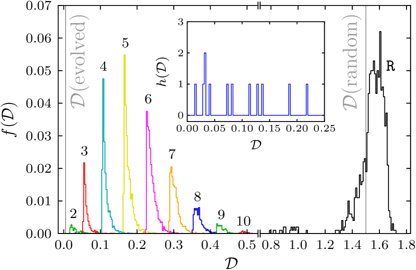
Figure 2: (Color online) Histogram of spectral distances in the reconstructed networks. Shown is the fraction $f({\mathcal{D}})$ of networks with spectral distance ${\mathcal{D}}$ to the evolution target reconstructed from the evolved networks (colored lines with number labels) and a random network of the same size (black line, labeled R). In the former, the different colors stand for different numbers of connected components $n_{\mathrm{c}}$, indicated by the numbers above the curves. Networks with $n_{\mathrm{c}}=1$ and $n_{\mathrm{c}}=11$ appear with very low frequencies. The (average) spectral distances of the original evolved and random networks are indicated by the vertical gray lines. The inset shows an enlarged segment of the histogram for $n_{\mathrm{c}}=1$, now in terms of absolute frequencies $h({\mathcal{D}})=f({\mathcal{D}})\times 10^{4}$.

In order to see how well the reconstructed networks reproduce the evolution target, i.e., the prescribed power-law scaling in the Laplacian spectrum, the first quantity to look at is the spectral distance ${\mathcal{D}}$ to the evolution target (defined in Eq. (3) of the Appendix). The value of ${\mathcal{D}}$ is lower the closer the Laplacian spectrum resembles the prescribed power law given by the value of ${d_{\mathrm{s}}}$. Figure 2 displays the distribution $f({\mathcal{D}})$ of the spectral distances for the reconstructed networks. For comparison, the distributions $\hat{P}(k)$, $\hat{P}(j,k)$, and $\hat{T}(k)$ were also calculated for an uncorrelated random network of the same size, the initial configuration of the evolutionary optimization. These distributions were used for the generation of 1000 realizations of reconstructed random networks by the same algorithm. The spectral distance of the reconstructed evolved networks is always higher than the average value of the evolved networks but significantly lower than the values of the random network and its reconstructed networks. Hence, the degree distribution and the two correlation measures together indeed encode the spectral behavior to a significant extent.

Remarkably, the distribution shows a structure of several, mostly well-separated peaks. As indicated by the different colors in Fig. 2, the multi-peak structure is generated by different numbers of connected components $n_{\mathrm{c}}$ in the reconstructed networks. Recall that a connected component of an undirected network is a subgraph in which any two vertices are connected to each other by paths, but are disconnected from all vertices in the other components. In the present context this means that a random walker diffusing on the network is confined to the connected component in which it started, and hence the diffusion processes on different components are independent. In contrast to the network evolution, which is explicitly constrained to produce a globally connected graph, the construction of the correlated random networks provides no possibility to control the number of components. Only a very small fraction of the resulting reconstructed networks, namely $12$ out of $10^{4}$, are found to be globally connected like the evolved networks. An explanation for the separation of the distribution into classes of equal number of connected components is that the number of components dictates the degeneracy of the smallest eigenvalue $\lambda_{1}=0$ and the smallest eigenvalues have the largest influence on the spectral distance. Notably, the globally connected networks with $n_{\mathrm{c}}=1$ deviate from the trend and do not exhibit spectral distances lower than those with $n_{\mathrm{c}}=2$. Due to the small number of realizations this observation can, however, not be considered as statistically significant.

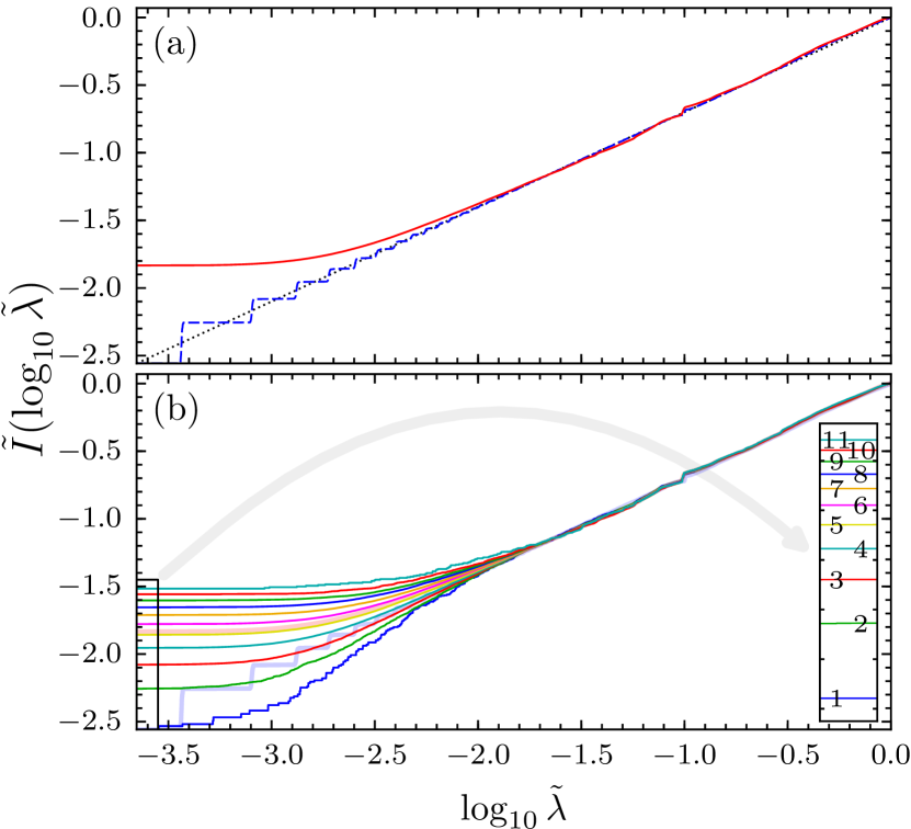
Figure 3: (Color online) Averaged logarithmically integrated Laplacian spectral density of reconstructed networks. In the upper panel (a), the averaged spectral densities of the evolved (dashed blue line) and the reconstructed (red line) networks are shown. The black dotted line displays the evolution target. The latter is broken down according to the number of connected components in the lower panel (b). The curves are labeled by their numbers of components in the inset, the color code is the same as in Fig. 2. For comparison, the transparent lines in the background show the curves of panel (a) again.

The influence of the small eigenvalues on the spectral distance is also clearly visible in the integrated spectral densities. Figure 3(a) displays the averaged logarithmically integrated spectral densities (defined in Eq. (2) of the Appendix) of the evolved and reconstructed networks. Evidently, the higher frequency of small eigenvalues is the main cause for the larger deviation from the target function. In Fig. 3(b) the spectral densities are individually averaged for the different classes of equal number of connected components. It shows how the deviation from the target function in the region of small eigenvalues indeed increases with the number of connected components in the network. The increasing degeneracy of the zero eigenvalue makes the integrated densities start out from higher values so that an increasing initial exceedance of the target function is inevitable. The integrated densities of the globally connected networks with $n_{\mathrm{c}}=1$ actually fall below the target function explaining the higher spectral distance than for $n_{\mathrm{c}}=2$ although the global trend of a lower initial value is continued. But again, due to the small number of realizations this observation should not be considered as statistically significant.

The shape of the spectral densities shown in Fig. 3(b) suggests a simple approximation that accounts for the positions of the peaks in the histogram of spectral distances in Fig. 2. Assuming that the spectral density exactly follows the target power law for large eigenvalues and becomes constant once the degeneracy $n_{c}$ of the minimal eigenvalue is reached, the evaluation of the spectral distance measure (3) yields the relation ${\mathcal{D}}(n_{c})=\frac{2}{3d_{s}}|\log(n_{c})|^{3}$, which is in good agreement with the numerical data for $n_{c}\geq 2$.

IV Reconstruction using partial information

Having seen that reconstructing the power-law Laplacian spectrum by using the degree distributions, degree-degree correlations, and degree-dependent clustering simultaneously works reasonably well, the question arises which out of these three measures is most relevant. In order to tackle this question, the distributions $\hat{P}(k)$, $\hat{P}(j,k)$, and $\hat{T}(k)$ extracted from the evolved networks are used as input for the four algorithms CM, Cl, Co, and Co-Cl. Again, this is done independently for $100$ realizations of the evolution and for each realization $100$ samples of random networks are generated.

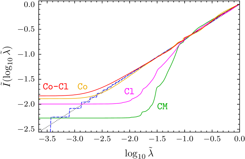
Figure 4: (Color online) Averaged logarithmically integrated Laplacian spectral densities of evolved networks (dashed blue) and reconstructions by the CM (green), Cl (magenta), Co (orange), and Co-Cl (red) algorithms. The black dotted line displays the evolution target.

Figure 4 shows the logarithmically integrated Laplacian spectral densities averaged over all $10^{4}$ samples for the four algorithms. First of all, we observe that for eigenvalues larger than a certain value (around $\log_{10}\tilde{\lambda}=-1$ which turns out to be the eigenvalue $\lambda=1$ ) all reconstruction algorithms reproduce the power law spectrum fairly well. Hence, the specification of the degree distribution appears to be sufficient for this part of the Laplacian spectrum. For smaller eigenvalues, the reconstructions by the CM and Cl algorithms, i.e., those algorithms not using the degree-degree correlations, deviate substantially. Networks constructed by the CM algorithm show the largest deviation from the power law while those generated by Cl lie slightly closer but differ in the same range of eigenvalues. In both cases the integrated spectral densities display several kink-like features which reflect accumulations of eigenvalues. A possible mechanism underlying such spectral degeneracies are network symmetries Karalus and Krug (2015). These features are absent from the spectra obtained using the Co and Co-Cl algorithms, which both resemble the target power law closely and almost equally well. Thus, the degree-degree correlations seem to be the major structural factor causing the scaling. The degree-dependent clustering has only a minor influence when the two-point correlations are reproduced as well.

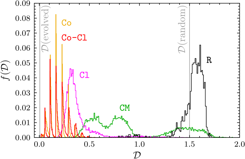
Figure 5: (Color online) Histogram of spectral distances for the networks reconstructed by all four algorithms. Shown is the fraction $f({\mathcal{D}})$ of networks with spectral distance ${\mathcal{D}}$ to the evolution target reconstructed from the evolved networks by the CM (green), Cl (magenta), Co (orange), and Co-Cl (red) algorithms. The black histogram (R) is the same as in Fig. 2 and the (average) spectral distances of the original evolved and random networks are indicated by the vertical gray lines.

For a quantification of this observation, Fig. 5 displays histograms of the spectral distances for all four reconstruction algorithms. As expected, the networks reconstructed by the Co and Co-Cl algorithms have the lowest spectral distances to the power-law spectrum. Both histograms are very similar and exhibit the characteristic multi-peak structure seen in Fig. 2. The spectral distances of the networks generated by Cl and CM are significantly larger, but even for the latter ones on average still lower than those of the reconstructed random networks.

One approach to avoid the inconveniences of handling not globally connected networks, such as the observed strong dependency of the spectral distance on the number of connected components, is to restrict the analysis to the largest components of the generated networks. By doing so, one presumes that the largest component represents the network as a whole and smaller components are less important. A major problem arises in the comparison of these restricted networks which will naturally all have different sizes. As the spectral distance depends inherently on the number of vertices $N$ there is no way to compare its values for networks of different sizes.

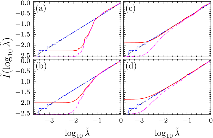
Figure 6: (Color online) Averaged logarithmically integrated Laplacian spectral densities of evolved networks (dashed blue), networks reconstructed by the (a) CM, (b) Cl, (c) Co, and (d) Co-Cl algorithms (red) as well as their largest components (dash-dotted magenta).

Nevertheless, the spectra can be calculated and visually compared. This is done in Fig. 6. The first observation is that the degeneracy of the smallest eigenvalue $\lambda=0$ is removed in the spectra of the largest components. In all four cases, the averaged logarithmically integrated spectral densities of the full networks and the respective largest components are qualitatively comparable. The deviations affect mainly the region of low eigenvalues where the integrated densities are significantly lower for the isolated largest components. In the CM and Cl reconstructions this results in a further deviation from the target power law. For the Co and Co-Cl reconstructions it might be difficult to tell if the spectra of the full networks or the isolated largest components lie “closer” to the target. However, the full networks resemble the power law over a larger range of eigenvalues than their largest components.

V Reconstruction of time series

In this section, the relevance of the different correlation measures in the evolutionary process shall be examined. To see if the degree distribution, degree-degree correlations, and degree-dependent clustering equally well characterize the network configurations at different stages of the evolution process, the reconstruction is applied to all intermediate steps of one exemplary evolution from a random graph towards the target spectral dimension of ${d_{\mathrm{s}}^{(1)}}=1.4$. As before, the distributions are extracted as absolute frequencies $\hat{P}(k)$, $\hat{P}(j,k)$, and $\hat{T}(k)$, now for each evolutionary time step. For each point in this time series, $100$ samples of the random (correlated) networks are generated independently by all four algorithms and analyzed.

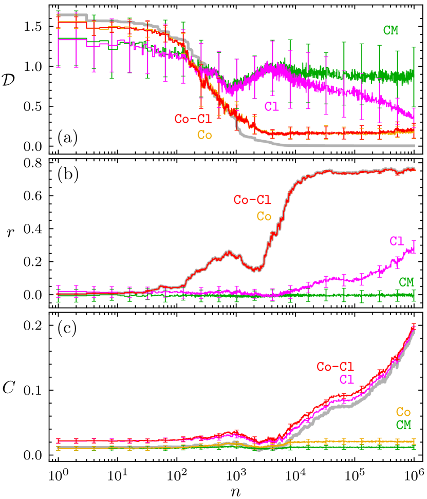
Figure 7: (Color online) Reconstruction averages of evolutionary time series by the CM (green), Cl (magenta), Co (orange), and Co-Cl (red) algorithms. Shown are (a) the spectral distance ${\mathcal{D}}$ to the evolution target, (b) the assortativity coefficient $r$, and (c) the global clustering coefficient $C$. All averages are calculated over 100 samples of the reconstruction and the error bars mark one standard deviation. The light gray curves in the background display the time series of the respective quantities in the evolving network.

The results of the time series reconstruction are summarized in Fig. 7 showing (a) the spectral distances ${\mathcal{D}}$, (b) the assortativity coefficients $r$, and (c) the global clustering coefficients $C$ of the reconstructed networks by all four algorithms at each time step $n$ of the evolution in comparison with the respective values from the network evolution. The spectral distances of all reconstructed networks are observed to take values in the same range as the evolving network for approximately the first $10^{2}$ evolution steps. For the reconstructions including the degree-degree correlations, i.e., the Co and Co-Cl algorithms, this trend continues for roughly another decade. Afterwards, from around $10^{3}$ evolution steps on, all reconstructed networks have larger spectral distances to the target power law than the evolving network itself with the Co and Co-Cl algorithms reaching significantly smaller values than CM and Cl. Additionally, after around $10^{4}$ evolution steps the spectral distance of the networks generated by Cl is observed to decrease. The reconstructions including the degree-degree correlations as input, Co and Co-Cl, exactly reproduce the assortativity coefficient of the evolving network, which increases and saturates to a rather high value after around $10^{4}$ evolutionary steps, throughout the time evolution. The CM algorithm generates non-assortative networks during the whole evolution while the networks constructed by the Cl algorithm show an increasing assortativity simultaneously with the observed decrease in the spectral distance in these networks after approximately $10^{4}$ evolutionary steps. The reconstructions including the degree-dependent clustering, Cl and Co-Cl, reproduce the increasing clustering coefficient of the evolution while the Co and CM algorithms generate networks with no transitivity.

These observations can be interpreted in the following way. In the initial phase of the evolution up to around $10^{2}$ evolution steps, slight improvements towards the power-law spectral densities are governed by the degree distribution. All reconstructions, including the CM algorithm, follow this trend. In the second phase up to around $10^{3}$ evolution steps, changes in the two-point correlations towards assortative structures are prevalent. These result in the largest reduction of the spectral distance. As only the Co and Co-Cl algorithms are able to reproduce this change they follow the reduction in the spectral distance. For the remaining evolution steps, more refined structural changes take place in the network evolution. These are not described by the degree distribution and correlation measures so that none of the algorithms is able to reproduce the improvement in the spectral distance. They are, however, accompanied by an increase in transitivity from around $10^{4}$ evolution steps on which is reproduced by the Cl and Co-Cl algorithms. This does not influence the spectral distance of the networks reconstructed by the Co-Cl algorithm. For the reconstruction by the Cl algorithm, the increase in transitivity is accompanied by an increase in assortativity and a decrease in the spectral distance at the same time. It is known that clustering and assortativity are correlated Ángeles Serrano and Boguñá (2005), so the observation is not surprising. In this way, the networks reconstructed by Cl indirectly acquire a higher assortativity which lets them “catch up” with the Co and Co-Cl reconstructions to some extent and also attain lower spectral distances.

VI Conclusions

We studied the importance of the distribution of vertex degrees and their correlations as basic structural measures in networks evolved towards a power-law Laplacian spectrum with a prescribed spectral dimension. To this end, random networks were generated and analyzed with the same degree distribution, degree-degree correlations, and degree-dependent clustering as the evolved networks. In this reconstruction procedure, the degree-degree correlations turned out to be the most important measure for the spectral scaling.

Figure 8: Typical configurations of reconstructed evolved networks making use of different correlation measures: (a) CM-algorithm, degree distribution only, (b) Cl-algorithm, degree distribution and degree-dependent clustering, (c) Co-algorithm, degree distribution and degree-degree correlations, and (d) Co-Cl-algorithm, degree distribution, degree-dependent clustering, and degree-degree correlations.

The evolved networks were predominantly characterized by a bimodal degree distribution and a high assortativity, i.e., positive degree-degree correlations. Additionally, an increasing transitivity, measured by the clustering coefficient, was observed. Together, they indicate a structural segregation into two distinct regions, densely connected cores and sparse peripheries. The results presented here confirm that assortativity is indeed the main structural feature of the evolved networks and higher order correlations, as measured by the degree-dependent clustering, play a minor role only. This interpretation is enforced by looking at typical realizations of the reconstructions from all four algorithms in Fig. 8: The Co- and Co-Cl-networks show signs of core-periphery structures as seen in the evolved networks (see Fig. 1) while the CM- and Cl-networks appear rather homogeneous. Secondly, it was observed that networks with a high clustering coefficient generated by the Cl algorithm appear to resemble the power-law spectrum better than those without (generated by the CM algorithm). This seems to be an indirect effect mediated by the correlations between assortativity and clustering: Networks with high clustering are known to be always assortative.

Finally, we remark that at this point we cannot answer the question why the observed core-periphery structures generate the power-law Laplacian spectra and, thus, anomalous diffusion behavior. In a different setting—where evolving networks were kept homogeneous—it was observed that networks with loops and dangling ends of different lengths are also able to generate such behavior Karalus and Krug (2015). A distribution of paths of different lengths through the network might as well be generated by the core-periphery structures found here. Just like in comb-like networks with power-law distributed teeth lengths Havlin and ben Avraham (2002) this interpretation provides an intuitive view on how the anomalous diffusion behavior is generated. The development of a minimal, analytically tractable model that elucidates the relationship between the core-periphery structure and the resulting power law spectrum seems highly desirable, but must be left to future work.

Appendix A Network evolution

Network evolution as a method to construct network structures with a prescribed power-law scaling in the Laplacian spectrum was successfully developed and described in Ref. Karalus and Porto (2012). The idea is to explore the configuration space of valid networks by successive steps of mutation and selection. In the basic setting, the mutation is realized by a random rewiring of one edge. The selection accepts this mutation if a spectral distance function ${\mathcal{D}}$ (called $\Delta$ in the original reference) is lowered and the network remains globally connected. In the following, the formal concepts of the network evolution are briefly summarized.

In order to represent the eigenvalue spectrum of the graph Laplacian, $\{\lambda_{\nu}\}_{\nu=1,\ldots,N}$, in a functional form the integrated spectral density

$$I(\lambda)=\frac{1}{N}\sum_{\nu=1}^{N}\Theta(\lambda-\lambda_{\nu})$$ (1)

is a convenient choice. Here, $\Theta$ denotes the Heaviside step function, $\Theta(x)=1$ for $x\geq 0$ and $\Theta(x)=0$ for $x<0$. Rescaling by the maximum eigenvalue, $\tilde{\lambda}_{\nu}=\lambda_{\nu}/\max_{\nu^{\prime}}\{\lambda_{\nu^{\prime}}\}$, does not change the scaling of $I$ but confines the eigenvalues to a finite interval, $0\leq\tilde{\lambda}_{\nu}\leq 1$. Power laws are most easily described on logarithmic scales. Therefore, the logarithmically integrated spectral density

$$\tilde{I}(\log\tilde{\lambda})=\log\left[\frac{1}{N}\sum_{\nu=1}^{N}\Theta(\log\tilde{\lambda}-\log\tilde{\lambda}_{\nu})\right]$$ (2)

is used such that a power-law target density $I^{\text{target}}(\lambda)\propto\lambda^{{d_{\mathrm{s}}}/2}$ appears as linear relation $\tilde{I}^{\text{target}}(\log\tilde{\lambda})=({d_{\mathrm{s}}}/2)\log\tilde{\lambda}$. The spectral distance ${\mathcal{D}}$ to the evolution target is defined as

$${\mathcal{D}}(\tilde{I},\tilde{I}^{\text{target}})=\int_{\log\tilde{\lambda}_{\min}^{\ast}}^{0}\left|\tilde{I}(\log\tilde{\lambda})-\tilde{I}^{\text{target}}(\log\tilde{\lambda})\right|^{2}\mathrm{d}\log\tilde{\lambda}\,.$$ (3)

The lower integration boundary $\log\tilde{\lambda}_{\min}^{\ast}$ is chosen such that $\tilde{I}^{\text{target}}(\log\tilde{\lambda}_{\min}^{\ast})=\log(N^{-1})$. For the numerical calculations in this work, the base 10 logarithm was used as denoted in the figures.

References

- Albert and Barabási (2002) R. Albert and A.-L. Barabási, Reviews of Modern Physics 74, 47 (2002).
- Dorogovtsev and Mendes (2002) S. N. Dorogovtsev and J. F. F. Mendes, Advances in Physics 51, 1079 (2002).
- Amaral and Ottino (2004) L. A. N. Amaral and J. M. Ottino, The European Physical Journal B - Condensed Matter and Complex Systems 38, 147 (2004).
- Newman (2010) M. E. J. Newman, Networks: An Introduction (Oxford University Press, New York, 2010).
- Atay et al. (2006) F. M. Atay, T. Bıyıkoğlu, and J. Jost, Physica D: Nonlinear Phenomena 224, 35 (2006).
- Almendral and Díaz-Guilera (2007) J. A. Almendral and A. Díaz-Guilera, New Journal of Physics 9, 187 (2007).
- Samukhin et al. (2008) A. N. Samukhin, S. N. Dorogovtsev, and J. F. F. Mendes, Physical Review E 77, 036115 (2008).
- van Mieghem (2011) P. van Mieghem, Graph spectra for complex networks (Cambridge University Press, New York, 2011).
- Jalan and Yadav (2015) S. Jalan and A. Yadav, Physical Review E 91, 012813 (2015).
- Grabow et al. (2015) C. Grabow, S. Grosskinsky, J. Kurths, and M. Timme, Physical Review E 91, 052815 (2015).
- Chung (1997) F. R. K. Chung, Spectral graph theory, no. 92 in Regional conference series in mathematics (American Mathematical Society, Providence, 1997).
- Arenas et al. (2008) A. Arenas, A. Díaz-Guilera, J. Kurths, Y. Moreno, and C. Zhou, Physics Reports 469, 93 (2008).
- Gurtovenko and Blumen (2005) A. Gurtovenko and A. Blumen, in Polymer Analysis, Polymer Theory (Springer, Berlin Heidelberg, 2005), no. 182 in Advances in Polymer Science, pp. 171–282.
- Havlin and ben Avraham (2002) S. Havlin and D. ben Avraham, Advances in Physics 51, 187 (2002).
- Noh and Rieger (2004) J. D. Noh and H. Rieger, Physical Review Letters 92, 118701 (2004).
- Bornholdt and Rohlf (2000) S. Bornholdt and T. Rohlf, Physical Review Letters 84, 6114 (2000).
- Oikonomou and Cluzel (2006) P. Oikonomou and P. Cluzel, Nature Physics 2, 532 (2006).
- Kashtan and Alon (2005) N. Kashtan and U. Alon, Proceedings of the National Academy of Sciences of the United States of America 102, 13773 (2005).
- Donetti et al. (2005) L. Donetti, P. I. Hurtado, and M. A. Muñoz, Physical Review Letters 95, 188701 (2005).
- Rad et al. (2008) A. A. Rad, M. Jalili, and M. Hasler, Chaos: An Interdisciplinary Journal of Nonlinear Science 18, 037104 (2008).
- Ipsen and Mikhailov (2002) M. Ipsen and A. S. Mikhailov, Physical Review E 66, 046109 (2002).
- Comellas and Diaz-Lopez (2008) F. Comellas and J. Diaz-Lopez, Physica A: Statistical Mechanics and its Applications 387, 6436 (2008).
- Erdős and Rényi (1959) P. Erdős and A. Rényi, Publicationes Mathematicae (Debrecen) 6, 290 (1959).
- Newman and Martin (2014) M. E. J. Newman and T. Martin, Physical Review E 90, 052824 (2014).
- Karalus and Porto (2012) S. Karalus and M. Porto, EPL (Europhysics Letters) 99, 38002 (2012).
- Newman (2002) M. E. J. Newman, Physical Review Letters 89, 208701 (2002).
- Newman (2003) M. E. J. Newman, Physical Review E 67, 026126 (2003).
- Newman et al. (2001) M. E. J. Newman, S. H. Strogatz, and D. J. Watts, Physical Review E 64, 026118 (2001).
- Watts and Strogatz (1998) D. J. Watts and S. H. Strogatz, Nature 393, 440 (1998).
- Vázquez et al. (2002) A. Vázquez, R. Pastor-Satorras, and A. Vespignani, Physical Review E 65, 066130 (2002).
- Molloy and Reed (1995) M. Molloy and B. Reed, Random Structures & Algorithms 6, 161 (1995).