Adaptive RBF-FD Method for Elliptic Problems with Point Singularities in 2D

Abstract

We describe and test numerically an adaptive meshless generalized finite difference method based on radial basis functions that competes well with the finite element method on standard benchmark problems with reentrant corners of the boundary, sharp peaks and rapid oscillations in the neighborhood of an isolated point. This is achieved thanks to significant improvements introduced into the earlier algorithms of [Oleg Davydov and Dang Thi Oanh, Adaptive meshless centers and RBF stencils for Poisson equation, Journal of Computational Physics, 230:287–304, 2011], including a new error indicator of Zienkiewicz-Zhu type.

1 Introduction

Let us consider the Dirichlet boundary value problem: Find $u:\overline{\Omega}\to\mathbb{R}$ such that

$$Lu=f\;\hbox{ on $\Omega$ },\quad u|_{\partial\Omega}=g,$$ (1)

where $L$ is a linear elliptic differential operator of second order, $\Omega\subset\mathbb{R}^{2}$ is a given bounded domain, the function $f$ is defined on $\Omega$, and the function $g$ is defined on the boundary $\partial\Omega$ of $\Omega$. A generalized finite difference discretization of the Dirichlet problem (1) is given by the following linear system with respect to the vector $\hat{u}=[\hat{u}_{\xi}]_{\xi\in\Xi}$:

$$\sum_{\xi\in\Xi_{\zeta}}w_{\zeta,\xi}\hat{u}_{\xi}=f(\zeta),\quad\zeta\in\Xi_{\rm int};\qquad\hat{u}_{\xi}=g(\xi),\quad\xi\in\partial\Xi,$$ (2)

where

• $\Xi\subset\overline{\Omega}$ is the set of discretization centers;

• $\hat{u}$ represents the approximation of the solution $u$ of (1) at the points $\xi\in\Xi$;

• $\partial\Xi:=\Xi\cap\partial\Omega$ is the set of boundary discretization centers;

• $\Xi_{\rm int}:=\Xi\setminus\partial\Xi$ is the set of interior discretization centers;

• $\Xi_{\zeta}$ is a set (called the stencil support of $\zeta$) that consists of the considered center $\zeta$ and some selected neighbor points $\xi_{i}\in\Xi$;

• $w_{\zeta,\xi}\in\mathbb{R}$ are the stencil weights chosen such that $\sum_{\xi\in\Xi_{\zeta}}w_{\zeta,\xi}u(\xi)$ is an approximation of $Lu(\zeta)$.

To set up the system (2), three tasks have to be addressed: (a) how to generate $\Xi$, (b) how to choose the stencil supports $\Xi_{\zeta}$, and (c) how to compute suitable weights $w_{\zeta,\xi}$.

In the RBF-FD method the weights $w_{\zeta,\xi}$, $\xi\in\Xi_{\zeta}$, are generated through the interpolation with radial basis functions. Referring to [3, 6] for further details and references, we briefly describe this approach. Let $\phi:\mathbb{R}_{+}\to\mathbb{R}$ be a positive definite radial basis function [2], for example the Gaussian function

$$\phi(r)=e^{-\varepsilon^{2}r^{2}},$$ (3)

where $\varepsilon$ is the shape parameter. Given $\zeta\in\Xi_{\rm int}$ and $\Xi_{\zeta}=\{\zeta_{0},\zeta_{1},\ldots,\zeta_{k}\}\subset\Xi$, with $\zeta_{0}=\zeta$, we set $\varphi_{i}(x)=\phi(\|x-\zeta_{i}\|)$, $x\in\mathbb{R}^{2}$, where $\|\cdot\|$ denotes the Euclidean norm in $\mathbb{R}^{2}$. Assuming for simplicity that the operator $L$ has the form

$$Lu(x)=\Delta u(x)+c(x)u(x),$$

we first find the weights $w_{i}$ such that

$$\Delta s(\zeta)=\sum_{i=0}^{k}w_{i}u(\zeta_{i}),$$

where $s(x):=\sum_{i=0}^{k}a_{i}\varphi_{i}(x)$, $a_{i}\in\mathbb{R}$, satisfies the interpolation condition $s(\zeta_{i})=u(\zeta_{i})$, $i=0,\ldots,k$. The vector $w=[w_{i}]_{i=0}^{k}$ can be computed by solving the linear system

$$\Phi_{\Xi_{\zeta}}w=[\Delta\varphi_{i}(\zeta)]_{i=0}^{k},\quad\text{with}\quad\Phi_{\Xi_{\zeta}}:=[\varphi_{j}(\zeta_{i})]_{i,j=0}^{k}.$$ (4)

In particular, for the Gaussian (3), we have

$$\Phi_{\Xi_{\zeta}}=[e^{-\varepsilon^{2}\|\zeta_{i}-\zeta_{j}\|^{2}}]_{i,j=0}^{k},\quad\Delta\varphi_{i}(\zeta)=4\varepsilon^{2}e^{-\varepsilon^{2}\|\zeta-\zeta_{i}\|^{2}}(\varepsilon^{2}\|\zeta-\zeta_{i}\|^{2}-1).$$ (5)

Assuming that the interpolant $s$ provides a good approximation of the function $u$, we expect that $\Delta u(\zeta)\approx\Delta s(\zeta)$, and thus

$$Lu(\zeta)\approx\sum_{i=0}^{k}w_{i}u(\zeta_{i})+c(\zeta)u(\zeta).$$

Therefore the weights $w_{\zeta,\xi}$ in (2) are chosen as follows:

$$w_{\zeta,\zeta}=w_{0}+c(\zeta),\qquad w_{\zeta,\zeta_{i}}=w_{i},\quad i=1,\ldots,k.$$

We refer to [5] for the bounds for the numerical differentiation error

$$\Big{|}Lu(\zeta)-\sum_{\xi\in\Xi_{\zeta}}w_{\zeta,\xi}u(\xi)\Big{|}.$$

The set of discretization centers $\Xi$ does not have to form a grid or mesh, therefore RBF-FD is a meshless method [9]. For more complicated problems it is advantageous to adapt the distribution of the centers to the features of the domain $\Omega$ and/or to the singularities of the solution $u$. This can be achieved through adaptive refinement of $\Xi$. In [3] we suggested a refinement algorithm and an algorithm for stencil support selection, leading to an effective meshless method capable of competing with the finite element method on a number of benchmark test problems. However, further experiments have shown certain deterioration of the approximation quality after many refinement steps, and suboptimal performance for more difficult test problems.

This motivated the current study, where both stencil support selection and refinement have been improved. The new algorithms presented in Sections 2 and 3 deliver the stencil supports $\Xi_{\zeta}$ with more evenly distributed points, and the adaptively selected sets $\Xi$ that better reflect the singularities of the solution. In the same time the improved method is more efficient because a costly post-processing step aimed at reducing the deterioration of the centers in the cause of subsequent refinements has been removed. One of the major differences in the refinement algorithm comparing to [3] is an error indicator of Zienkiewicz-Zhu type used instead of a simple gradient estimate. This leads to a significant improvement of the performance of the adaptive RBF-FD method for more difficult problems. Section 4 is devoted to numerical experiments with the test problems considered previously in [3], several test problems suggested in [8] as benchmarks for testing adaptive grid refinement, and a problem on a domain with a circular slit. In this paper we concentrate on the elliptic problems with point singularities, such as the reentrant corners of the boundary, sharp peaks and oscillations in the neighborhood of an isolated point. Problems with line or curve singularities, boundary layers and wave fronts require further adjustments of the algorithms taking into account the anisotropy of the solution $u$ and will be considered elsewhere. As in [3], comparison is provided with the numerical results obtained with the adaptive finite element method of MATLAB PDE Toolbox [11]. The results confirm the robust and competitive performance of the suggested method for problems with point singularities. A conclusion is given in Section 5.

2 Meshless stencil support selection

Given $\zeta\in\Xi_{\rm int}$, let $\Xi_{\zeta}=\{\zeta,\zeta_{1},\ldots,\zeta_{n}\}\subset\Xi$, where the points $\zeta_{1},\ldots,\zeta_{n}$ are ordered counterclockwise with respect to $\zeta$. Following [3, Section 5], we set

$$\mu(\zeta_{1},\ldots,\zeta_{n}):=\sum_{i=1}^{n}\alpha_{i}^{2},\quad\underline{\alpha}(\zeta_{1},\ldots,\zeta_{n}):=\min_{1\leq i\leq n}\alpha_{i},\quad\overline{\alpha}(\zeta_{1},\ldots,\zeta_{n}):=\max_{1\leq i\leq n}\alpha_{i},$$

where $\alpha_{i}$ denotes the angle between the rays $\zeta\zeta_{i}$, $\zeta\zeta_{i+1}$ in the counterclockwise direction, with the cyclic identification $\zeta_{n+i}:=\zeta_{i}$. Since $\sum_{i=1}^{n}\alpha_{i}=2\pi$, the minimum of the expression $\sum_{i=1}^{n}\alpha_{i}^{2}$ is attained for the uniformly spaced directions $\zeta\zeta_{i}$ such that the angles $\alpha_{i}$ are all equal $\alpha_{1}=\cdots=\alpha_{n}=2\pi/n$. Although we cannot expect this minimum to be achieved for some subset $\{\zeta_{1},\ldots,\zeta_{n}\}$ of the finite set $\Xi$, we use $\mu$ as a measure of angle uniformity when comparing two subsets of this type. We prefer $\mu$ over the possible alternative measure $\overline{\alpha}/\underline{\alpha}$ that has the drawback that it does not ‘see’ small improvements in the uniformity that do not affect either minimum or maximum angle. It is however convenient to use it for a termination criterion

$$\overline{\alpha}(\zeta_{1},\ldots,\zeta_{n})\leq v\,\underline{\alpha}(\zeta_{1},\ldots,\zeta_{n}),$$ (6)

with some tolerance $v>1.0$. Starting with $k$ nearest points, we replace $\zeta_{j}$’s one after another by the more distant points $\xi\in\Xi\setminus\Xi_{\zeta}$ so that $\mu(\zeta_{1},\ldots,\zeta_{k})$ becomes smaller. On the other hand, since nearby points are preferable, we introduce the second termination criterion

$$\|\zeta-\xi\|\geq\frac{c}{2\,k}\sum_{j=1}^{k}\big{(}\|\zeta_{j}-\zeta\|+\|\zeta_{j}-\zeta_{j+1}\|\big{)},$$ (7)

with a tolerance $c>1.0$ for the exchange candidate $\xi\in\Xi\setminus\Xi_{\zeta}$.

Empirically chosen values $v=2.5$ and $c=3.0$ work well in all our numerical experiments, where we always choose $k=6$ to guarantee that the density of the system matrix of (2) is comparable to the density of the system matrix of the conforming finite element method with linear shape functions, see [3]. For the sake of efficiency we search initially for $m=50$ nearest points, and double the size of the local cloud each time it has been exhausted.

Algorithm 1.

Meshless stencil support selection
Input: $\Xi$, $\zeta$. Output: $\Xi_{\zeta}$. Parameters: $k$ (the number of points in $\Xi_{\zeta}\setminus\{\zeta\}$), $v>1.0$ (the angle uniformity tolerance), $c>1.0$ (distance tolerance), and $m>k$ (the increment size of the local cloud). Parameter values used in our numerical experiments: $k=6$, $v=2.5$, $c=3.0$ and $m=50$.

1. Find $m$ nearest points $\xi_{1},\ldots,\xi_{m}$ in $\Xi\setminus\{\zeta\}$ to $\zeta$, sorted by increasing distance to $\zeta$, and initialize $\Xi_{\zeta}:=\{\zeta,\zeta_{1},\ldots,\zeta_{k}\}=\{\zeta,\xi_{1},\ldots,\xi_{k}\}$ and $i:=k+1$.

2. While $i\leq m$:

   1. If $\|\zeta-\xi_{i}\|\geq\frac{c}{2\,k}\sum_{j=1}^{k}\big{(}\|\zeta_{j}-\zeta\|+\|\zeta_{j}-\zeta_{j+1}\|\big{)}$, then STOP and return $\Xi_{\zeta}$.

   2. Compute the angles $\alpha^{\prime}_{1},\ldots,\alpha^{\prime}_{k+1}$ formed by the extended set $\{\zeta^{\prime}_{1},\ldots,\zeta^{\prime}_{k+1}\}=\{\zeta_{1},\ldots,\zeta_{k},\xi_{i}\}$. If both angles between $\zeta\xi_{i}$ and its two neighboring rays are greater than the minimum angle $\underline{\alpha}^{\prime}:=\underline{\alpha}(\zeta^{\prime}_{1},\ldots,\zeta^{\prime}_{k+1})$:

      1. Find $j$ such that $\alpha^{\prime}_{j}=\underline{\alpha}^{\prime}$. Choose $p=j$ or $p=j+1$ depending on whether $\alpha^{\prime}_{j-1}<\alpha^{\prime}_{j+1}$ or $\alpha^{\prime}_{j-1}\geq\alpha^{\prime}_{j+1}$.

      2. If $\mu(\{\zeta^{\prime}_{1},\ldots,\zeta^{\prime}_{k+1}\}\setminus\{\zeta^{\prime}_{p}\})<\mu(\zeta_{1},\ldots,\zeta_{k})$:

         1. Update $\Xi_{\zeta}:=\{\zeta,\zeta_{1},\ldots,\zeta_{k}\}=\{\zeta,\zeta^{\prime}_{1},\ldots,\zeta^{\prime}_{k+1}\}\setminus\{\zeta^{\prime}_{p}\}$.

         2. If $\overline{\alpha}(\zeta_{1},\ldots,\zeta_{k})\leq v\,\underline{\alpha}(\zeta_{1},\ldots,\zeta_{k})$, then STOP and return $\Xi_{\zeta}$.

   3. If $i=m$:

      1. Find the next $m$ nearest points $\xi_{m+1},\ldots,\xi_{2m}$ in $\Xi\setminus\{\zeta\}$ to $\zeta$, sorted by increasing distance to $\zeta$, and set $m:=2m$.

   4. Set $i:=i+1.$

Remarks

1. In the earlier version of our algorithm [3, Algorithm 1] we used a point cloud with a fixed number ($m=30$) of nearest points considered for the inclusion into $\Xi_{\zeta}$, which sometimes led to the termination with rather non-uniform angles $\alpha_{i}$. This was in part compensated by the removal of the ‘worst’ point in this situation. In the improved algorithm of this paper we dropped this removal step, and added the second termination criterion (7) in Step II.1, while allowing potentially any point of $\Xi$ to be selected into $\Xi_{\zeta}$. Theoretically, the algorithm may continue until all points in $\Xi$ are exhausted such that neither (6) nor (7) is satisfied. This however, never happened in our experiments. Note that Algorithm 1 is supposed to work in the interaction with the adaptive refinement according to Algorithm 2, and so its behavior may be quite different if it is applied to a set $\Xi$ of a different nature.

2. The choice of $p$ in Step II.2.i ensures that

   $$\mu\big{(}\{\zeta^{\prime}_{1},\ldots,\zeta^{\prime}_{k+1}\}\setminus\{\zeta^{\prime}_{p}\}\big{)}=\min\Big{\{}\mu\big{(}\{\zeta^{\prime}_{1},\ldots,\zeta^{\prime}_{k+1}\}\setminus\{\zeta^{\prime}_{j}\}\big{)},\;\mu\big{(}\{\zeta^{\prime}_{1},\ldots,\zeta^{\prime}_{k+1}\}\setminus\{\zeta^{\prime}_{j+1}\}\big{)}\Big{\}}.$$

3. For non-convex domains the points $\xi_{i}$ such that the segment between $\zeta$ and $\xi_{i}$ intersects the domain boundary are ignored in Step I and Step II.3.

4. Due to certain oversampling of the boundary by Algorithm 2, see Remark no. 3 after it, many of the nearest centers to $\zeta$ may lie on a straight segment of the boundary. Since these points are not desirable in $\Xi_{\zeta}$, we switch off the termination in Step II.1 in case when the number of such points in the current set $\Xi_{\zeta}$ is more than 3. However, this rule is not applied if $i\geq 50$, in order to avoid inclusion of very far points.

Figures 1(a–d) show typical stencil supports $\Xi_{\zeta}$ obtained by Algorithm 1 in our experiments. The choice of parameters $c$ and $v$ determines the trade-off between improving the uniformity of the angles $\alpha_{i}$ and avoiding far away points. Figure 1(e) shows an example of $\Xi_{\zeta}$ for which Algorithm 1 terminates at Step II.1. The red cross indicates the center $\xi_{i}$ for which the termination condition (7) is satisfied ($i=52$), and hence the improvement of the angles is terminated. In fact $\overline{\alpha}/\underline{\alpha}=4.3343>v$ in this case. Figure 1(f) gives an example of the other extreme, where the termination is at Step II.2.ii.b so that $\overline{\alpha}/\underline{\alpha}=2.4410<v$, but this is achieved at the expense of including in $\Xi_{\zeta}$ a rather distant center (the circled dot near the bottom).

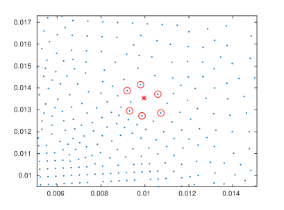
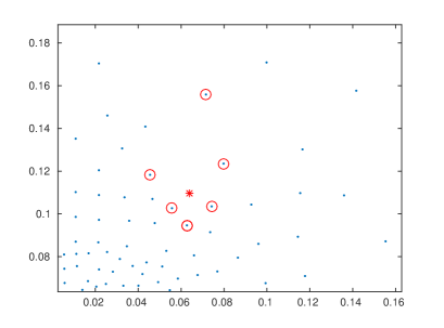
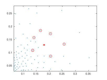
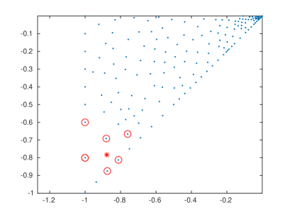
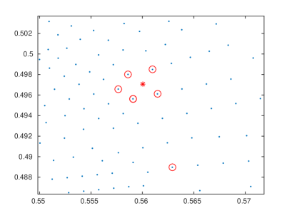
Figure 1: Stencil supports $\Xi_{\zeta}$ obtained by Algorithm 1: The star shows the position of $\zeta$ and the circles the positions of $\xi_{1}\ldots,\xi_{6}$.

In order to quantify the uniformity of the stencil supports produced by Algorithm 1, we define several measures as follows. Given a set of stencil supports $\Xi_{\zeta}=\{\zeta,\zeta_{1},\ldots,\zeta_{n}\}$, we denote by $v_{\mathrm{max}}$ the maximum and by $v_{\mathrm{aver}}$ the average values of the quotient $\overline{\alpha}/\underline{\alpha}$ over all $\Xi_{\zeta}$ in this set. Similarly, $c_{\mathrm{max}}$ and $c_{\mathrm{aver}}$ denote the maximum and the average values of the quotient

$$\max_{j=1,\ldots,n}\|\zeta-\zeta_{j}\|\Big{/}\frac{1}{2\,n}\sum_{j=1}^{n}\big{(}\|\zeta_{j}-\zeta\|+\|\zeta_{j}-\zeta_{j+1}\|\big{)}.$$ (8)

The values of these measures in our experiments are provided in Table 3 at the end of Section 4, see there a discussion of the results as well.

3 Refinement method

Before giving a formal description of our algorithm we discuss its main features and changes in comparison to [3, Algorithm 2].

Error indicator. Assuming that an approximate discrete solution $\hat{u}$ of the Dirichlet problem (1) is determined via (2) with some $\Xi$ and stencil supports $\Xi_{\zeta}$ for all $\zeta\in\Xi_{\rm int}$, we choose an error indicator $\varepsilon(\zeta,\xi)$ associated with each ‘edge’ $\zeta\xi$ for all $\zeta\in\Xi_{\rm int}$ and $\xi\in\Xi_{\zeta}\setminus\{\zeta\}$. In our earlier refinement algorithm [3, Section 6] we used $\varepsilon(\zeta,\xi)=\varepsilon_{0}(\zeta,\xi):=|\hat{u}_{\zeta}-\hat{u}_{\xi}|$. However, this indicator identifies the areas where the gradient of the solution is big, which results in some cases, see Figure 14 and related discussion in Section 4, in oversampling relatively flat regions and undersampling the regions of high curvature, which leads to sub-optimal solution. Therefore we replace it by an indicator of Zienkiewicz-Zhu type that estimates the error of the approximation of the directional derivative along the edge $\zeta\xi$. The error indicator used in this paper is defined as follows. For each $\zeta\in\Xi_{\rm int}$, let $\ell_{\zeta}(x)=a+b^{T}(x-\zeta)$ be the linear polynomial that fits the data $\{(\xi,\hat{u}_{\xi}):\xi\in\Xi_{\zeta}\}$ in the least squares sense, that is its coefficients $a\in\mathbb{R}$, $b\in\mathbb{R}^{2}$ are chosen such that the sum

$$\sum_{\xi\in\Xi_{\zeta}}|\hat{u}_{\xi}-\ell_{\zeta}(\xi)|^{2}$$

is minimized. (This minimization problem has a unique solution as soon as $\Xi_{\zeta}$ is not a subset of a straight line.) We set

$$\varepsilon(\zeta,\xi)=\varepsilon_{1}(\zeta,\xi):=|(\hat{u}_{\zeta}-\hat{u}_{\xi})-(\ell_{\zeta}(\zeta)-\ell_{\zeta}(\xi))|,\quad\zeta\in\Xi_{\rm int},\;\xi\in\Xi_{\zeta}\setminus\{\zeta\}.$$ (9)

We can interprete $\varepsilon_{1}(\zeta,\xi)$ as an edge-based indicator of averaging type. Indeed, $(\hat{u}_{\zeta}-\hat{u}_{\xi})/\|\zeta-\xi\|$ is an estimate of the directional derivative of the solution based only on two points $\zeta,\xi$, whereas $(\ell_{\zeta}(\zeta)-\ell_{\zeta}(\xi))/\|\zeta-\xi\|$ is an estimate of the same directional derivative based on averaging the information from all points in $\Xi_{\zeta}$. In the finite element method such error indicators are usually based on averaging the gradient over elements, see [14, 10]. Instead, in our meshless setting we naturally resort to directional derivatives and edges.

Marking strategy. The refinement of $\Xi$ is achieved by inserting one or more new centers in the vicinity of each edge $\zeta\xi$ marked for refinement. An overview of marking methods employed in the finite element adaptive refinement algorithms can be found in [10]. As in [3] we follow the so called ‘maximum strategy’ applied to edges rather than elements. Therefore the main condition for the edge $\zeta\xi$ to be refined is

$$\varepsilon(\zeta,\xi)\geq\gamma\bar{\varepsilon}(\Xi),\quad\text{where}\;\bar{\varepsilon}(\Xi):=\max\{\varepsilon(\zeta,\xi):\,\zeta\in\Xi_{\rm int},\,\xi\in\Xi_{\zeta}\},$$ (10)

and $\gamma\in(0,1)$ is a prescribed tolerance. We also follow the common practice of preventing that too few new centers are generated in one refinement step by reducing the threshold for $\varepsilon(\zeta,\xi)$ and marking further edges in the event that the number of the new interior centers is less that certain percentage of the total number of centers in $\Xi_{\rm int}$, see Step III of Algorithm 2.

Refinement in the vicinity of a marked edge. For each marked edge $\zeta\xi$, the candidate new centers in [3, Algorithm 2] are the middle point $\xi_{\rm mid}=(\zeta+\xi)/2$ of the edge, as well as two neighboring points on the boundary should $\xi$ be a boundary center. To make the local distribution of centers more uniform and isotropic, we now also consider the points $\xi_{\rm mid}^{\pm}:=\xi_{\rm mid}\pm d\bar{\nu}$, where $d=\|\zeta-\xi\|/2$ and $\bar{\nu}$ is the unit vector perpendicular to the edge $\zeta\xi$, as candidate new centers, see Figure 2.

Figure 2: Centers to be added in the vicinity of a marked edge.

As in [3], we only proceed with the refinement if

$$\operatorname{dist}(\xi^{\prime},\Xi^{\prime})\geq\mu\operatorname{sep}_{\xi^{\prime}}(\Xi^{\prime}),\quad\text{with a prescribed tolerance $\mu\in(0,1)$,}$$ (11)

that is, if the insertion of a new center $\xi^{\prime}$ into the current set $\Xi^{\prime}$ does not significantly reduce the local separation defined as

$$\operatorname{sep}_{\xi^{\prime}}(\Xi^{\prime}):=\frac{1}{4}\sum_{i=1}^{4}\operatorname{dist}(\xi_{i},\Xi^{\prime}\setminus\{\xi_{i}\}),$$ (12)

where $\xi_{1},\ldots,\xi_{4}$ are the four closest points in $\Xi^{\prime}$ to $\xi^{\prime}$, and $\operatorname{dist}(x,Y):=\inf\{\|x-y\|:\,y\in Y\}$ is the distance from a point $x$ to a set $Y$. Moreover, we also check that $\xi^{\prime}\notin\partial\Omega$ is not placed too close to the boundary, see Steps II.2 and II.3.i of Algorithm 2.

Algorithm 2.

Adaptive meshless refinement
Input: The set of centers $\Xi$ and stencil supports $\{\Xi_{\zeta}:\,\zeta\in\Xi_{\rm int}\}$.
Output: The refined set of centers $\Xi^{\prime}$.
Parameters: $\gamma=0.5$ (error indicator tolerance), $\mu=0.8$ (separation tolerance) and $n=15$ (percentage of added centers).

1. Compute the error indicator threshold $\bar{\varepsilon}=\gamma\bar{\varepsilon}(\Xi)$ and initialize $\Xi^{\prime}:=\Xi$.

2. For each edge $\zeta\xi$, $\zeta\in\Xi_{\rm int}$, $\xi\in\Xi_{\zeta}\setminus\{\zeta\}$, such that $\varepsilon(\zeta,\xi)\geq\bar{\varepsilon}$:

   1. Compute $\xi_{\rm mid}:=(\zeta+\xi)/2$, $\xi_{\rm mid}^{+}:=\xi_{\rm mid}+d\bar{\nu}$ and $\xi_{\rm mid}^{-}:=\xi_{\rm mid}-d\bar{\nu}$, where $d:=\|\zeta-\xi\|/2$ and $\bar{\nu}$ is the unit vector perpendicular to the edge $\zeta\xi$.
      Initialize $\Xi_{C}:=\emptyset$.

   2. If $\xi\in\Xi_{\rm int}$, then for each $\xi^{\prime}\in\{\xi_{\rm mid},\xi_{\rm mid}^{+},\xi_{\rm mid}^{-}\}$:

      1. If $\operatorname{dist}(\xi^{\prime},\partial\Omega)\geq d/2$ and $\operatorname{dist}(\xi^{\prime},\Xi^{\prime})\geq\mu\operatorname{sep}_{\xi^{\prime}}(\Xi^{\prime})$, then set $\Xi_{C}:=\Xi_{C}\cup\{\xi^{\prime}\}$.

   3. ElseIf $\xi\in\partial\Xi$:

      1. For each $\xi^{\prime}\in\{\xi_{\rm mid},\xi_{\rm mid}^{+},\xi_{\rm mid}^{-}\}$:
         If $\operatorname{dist}(\xi^{\prime},\partial\Omega)\geq d/2$ and $\operatorname{dist}(\xi^{\prime},\Xi^{\prime})\geq d/2$, then set $\Xi_{C}:=\Xi_{C}\cup\{\xi^{\prime}\}$.

      2. If $\Xi_{C}\neq\emptyset$ or $\operatorname{dist}(\xi_{\rm mid},\partial\Omega)<d/2$:
         Find two neighbors $\xi_{-},\xi_{+}$ of $\xi$ in $\partial\Xi$, one in each direction from $\xi$ along the boundary, and compute two middle points $\xi^{\prime}_{-},\xi^{\prime}_{+}\in\partial\Omega$ defined by the pairs $\xi,\xi_{-}$ and $\xi,\xi_{+}$, respectively. Set $\Xi_{C}:=\Xi_{C}\cup\{\xi^{\prime}_{+},\xi^{\prime}_{-}\}$.

   4. Set $\Xi^{\prime}:=\Xi^{\prime}\cup\Xi_{C}$.

3. If the number of centers in $\Xi^{\prime}_{\rm int}\setminus\Xi_{\rm int}$ is less than $n$% of the number of centers in $\Xi_{\rm int}$, then set $\bar{\varepsilon}:=\gamma\bar{\varepsilon}$ and goto Step II.
   Else STOP and return $\Xi^{\prime}$.

Remarks

1. Algorithm 2 is applied recursively starting from an initial non-adaptive set of centers $\Xi$. In our experiments in Section 4 it is the set of centers of the initial finite element mesh created by MATLAB PDE Toolbox with default parameters.

2. The middle points in Step II.3.ii are found using the parameterizations of the respective boundary components connecting $\xi$ with either $\xi_{-}$ or $\xi_{+}$. If the middle point $\xi^{\prime}_{-}$ or $\xi^{\prime}_{+}$ is already in $\Xi^{\prime}$, it is not added again, which is easy to avoid by keeping track of the pairs of centers on the boundary that have been refined.

3. Generally, our algorithm leads to a slight oversampling of the boundary, which can be seen in the numerical results in Section 4. This is generally harmless because the boundary centers do not bear any degrees of freedom and hence the size of the system matrix does not increase. However, this leads to certain difficulties for Algorithm 1, see Remark no. 4 after it. To reduce the oversampling, in the experiments below we avoid adding one or both points $\xi^{\prime}_{-},\xi^{\prime}_{+}$ in Step II.3.ii in the following situations:

   • $\xi^{\prime}_{-}$ is not added to $\Xi_{C}$ if $\|\xi^{\prime}_{-}-\xi_{\rm mid}\|\geq\|\xi^{\prime}_{+}-\xi_{\rm mid}\|$, $\|\xi^{\prime}_{-}-\xi\|\leq\min\{d,2\|\xi^{\prime}_{+}-\xi\|\}$ and $\|\xi-\xi^{\prime}_{-}\|+\|\xi-\xi^{\prime}_{+}\|\leq 2\|\xi^{\prime}_{+}-\xi^{\prime}_{-}\|$.

   • $\xi^{\prime}_{+}$ is not added to $\Xi_{C}$ if $\|\xi^{\prime}_{+}-\xi_{\rm mid}\|\geq\|\xi^{\prime}_{-}-\xi_{\rm mid}\|$, $\|\xi^{\prime}_{+}-\xi\|\leq\min\{d,2\|\xi^{\prime}_{-}-\xi\|\}$ and $\|\xi-\xi^{\prime}_{-}\|+\|\xi-\xi^{\prime}_{+}\|\leq 2\|\xi^{\prime}_{+}-\xi^{\prime}_{-}\|$.

4. To get faster convergence of the numerical solution for easier problems, we enforce a reduction of the error indicator threshold $\bar{\varepsilon}$ between subsequent applications of Algorithm 2. Let $\bar{\varepsilon}_{\rm prev}$ be the threshold used for the previous refinement, and let $\bar{\varepsilon}$ be the value computed at Step I of the current refinement. If $\bar{\varepsilon}_{\rm prev}<\bar{\varepsilon}$, then we replace $\bar{\varepsilon}$ by $\bar{\varepsilon}:=\bar{\varepsilon}_{\rm prev}/2$, and proceed to Step II as usual. This procedure is used in the numerical experiments for Test Problems 1, 2 and 3 with $\omega=\pi+0.01,5\pi/4,7\pi/4$. Moreover, in this case we use $n=5$ instead of the default $n=15$ which helps to get smoother error curves. The value $n=5$ for the percentage of the added centers is also used for Test Problem 3 with $\omega=2\pi$ and Test Problem 4.

5. Note that the current algorithm no longer requires an (expensive) post-processing as in Step III of [3, Algorithm 2].

4 Numerical results

To illustrate the performance of the improved algorithms, we consider a number of benchmark test problems where adaptively refined centers are known to be of great advantage, and compare our results with those obtained with the help of the PDE Toolbox [11] using the finite element method with piecewise linear shape functions and default parameters of the adaptive refinement. This comparison is fair because the density of the system matrices resulting from our method is close to the density of the system matrices of such finite element method thanks to the fact that we choose $k=6$ points in the stencil supports of Algorithm 1. We refer to [3] for a detailed discussion and numerical results on the density of the system matrices.

We use the RBF-FD weights $w_{\zeta,\xi}$, $\xi\in\Xi_{\zeta}$, with Gaussian function (3) described in the introduction. Our investigation in [4] has shown that small values of the shape parameter $\varepsilon$ in (3) lead to reliable, albeit not always optimal results. For simplicity we use a fixed small value $\varepsilon=10^{-5}$ and compute the weights $w_{\zeta,\xi}$ by the Gauss-QR method as described in [4], see also [7]. Note that in [3, 4] we added a constant term to the Gaussian form to ensure that the scheme is exact for constants. This however turns out to be insignificant for the performance of the method as can be seen from the numerical results in this paper. The constant term causes certain technical complications for the computation of the weights by the Gauss-QR method, see [4].

As a measure of the quality of the results we use the root mean square (rms) error $E_{c}$ of the solution $\hat{u}$ of (2) against the exact solution $u$ of (1) on the centers,

$$E_{c}=\Big{(}\frac{1}{N}\sum_{\zeta\in\Xi_{\rm int}}(\hat{u}_{\zeta}-u(\zeta))^{2}\Big{)}^{1/2}.$$ (13)

where $N=\#\Xi_{\rm int}$ is the number of interior discretization centers. For the finite element method the set $\Xi_{\rm int}$ consists of all interior vertices of the triangulation. Since these sets are different for both methods, we also compute the rms error $E_{g}$ on a fixed uniform grid with step size $0.001$, where the values of the approximate solution $\hat{u}$ at the grid points are obtained by evaluating the piecewise linear interpolant with respect to the Delaunay triangulation of the centers.

The first two test problems have been considered in [3], see Test Problems 2 and 3 of that paper.

Test Problem 1.

Laplace equation $\Delta u=0$ in the circle sector $\Omega$ given by the inequalities $r<1$, $-3\pi/4<\varphi<3\pi/4$ in polar coordinates, with Dirichlet boundary conditions defined by $u(r,\varphi)=\cos(2\varphi/3)$ along the arc, and $u(r,\varphi)=0$ along the straight lines. The exact solution is $u(r,\varphi)=r^{2/3}\cos(2\varphi/3)$.

Test Problem 2.

Laplace equation $\Delta u=0$ in the domain $\Omega=(0.01,1.01)^{2}$ with Dirichlet boundary conditions chosen such that the exact solution is $u(x,y)=\log(x^{2}+y^{2})$.

The solutions of both problems have a singularity at the origin, as illustrated in Figure 3. Our numerical results for these problems are presented in Figures 4–6.

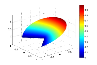
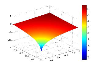
Figure 3: Exact solutions of Test Problems 1 (left) and 2 (right).

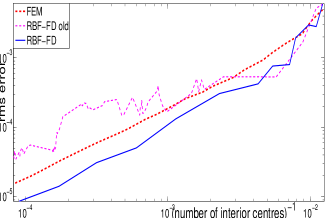
(a) Errors on centers

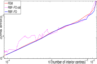
(b) Errors on grid

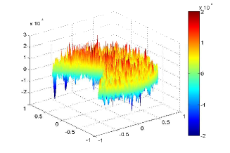
(c) RBF-FD error

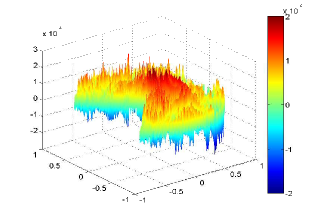
(d) FEM error

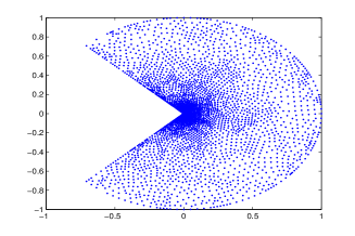
(e) RBF-FD centers (3169)

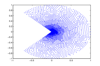
(f) FEM centers (3009)

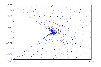
(g) RBF-FD centers: zoom

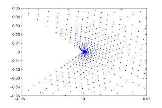
(h) FEM centers: zoom

Figure 4: Test Problem 1: (a) Error $E_{c}$ of the discrete solution on the centers generated by consecutive refinements with the respective method, using FEM and two versions of the RBF-FD method (RBF-FD old: the method of [3], RBF-FD: the method of this paper) as function of the reciprocal of the number of interior centers. (b) Error $E_{g}$ of the interpolated solutions on a uniform grid. (cd) Error function $u-\hat{u}$ for the RBF-FD solution of this paper on 3169 interior centers and the FEM solution on 3009 interior vertices. (ef) The centers used for the respective solutions. (gh) Zooms into both sets of centers.

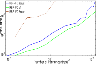
(a) Errors on centers

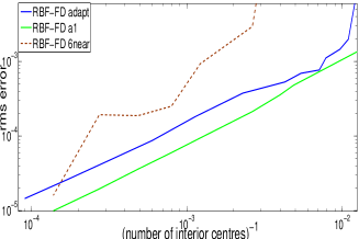
(b) Errors on grid

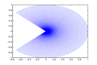
(c) Centers (3654)

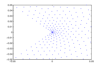
(d) Centers: zoom

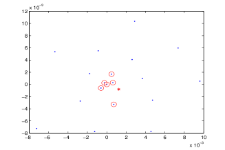
(e) $\Xi_{\zeta}$ for RBF-FD 6near

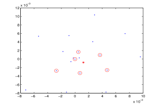
(f) $\Xi_{\zeta}$ by Algorithm 1

Figure 5: Test Problem 1: Results on smoothly distributed centers obtained by a priori refinement using DistMesh. (ab) Errors on the centers and on a uniform grid as in Figure 4. Two methods on smooth centers, RBF-FD method with stencil support selection according to Algorithm 1 (RBF-FD a1) and RBF-FD method with stencil supports $\Xi_{\zeta}$ obtained by choosing $\zeta$ and its 6 nearest points in $\Xi$ (RBF-FD 6near). The plots also include for comparison the error curves for the adaptive RBF-FD method of Figure 4 (RBF-FD adapt). (cd) The 3654 centers obtained by DistMesh with $h_{0}=0.0007$ and $\beta=0.5$, and a zoom. (ef) Example where $\Xi_{\zeta}$ obtained by Algorithm 1 is significantly different from 6 nearest points.

$\#\Xi_{\rm int}$	205	250	378	818	1255	2057	3654	7226
$h_{0}$	0.0007	0.0007	0.001	0.0012	0.00065	0.0012	0.0007	0.0013
$\beta$	0.700	0.675	0.650	0.600	0.575	0.525	0.500	0.425

Table 1: Parameters of distmesh2d.m used to produce the a priori sets of centers for Test Problem 1: $\#\Xi_{\rm int}$ is the number of interior centers, $h_{0}$ the initial edge length, and $\beta$ the power of the scaled edge length function in the form $\sigma(r)=r^{\beta}$. The set with $\#\Xi_{\rm int}=3654$ is illustrated in Figure 5(cd).

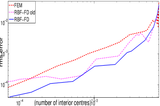
(a) Errors on centers

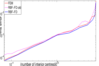
(b) Errors on grid

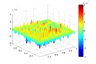
(c) RBF-FD error

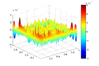
(d) FEM error

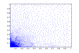
(e) RBF-FD centers (1938)

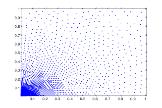
(f) FEM centers (1811)

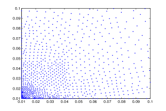
(g) RBF-FD centers: zoom

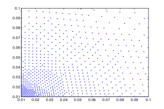
(h) FEM centers: zoom

Figure 6: Test Problem 2: Errors and centers as in Figure 4. The plots in (cd) are based on the RBF-FD solution on 1938 interior centers shown in (e) and the FEM solution on 1811 interior vertices shown in (f).

Figures 4(ab) and 6(ab) show the graphs of the rms errors $E_{c}$ and $E_{g}$ of the RBF-FD method in comparison to the finite element method, as function of the reciprocal of the number of interior centers. The curves labeled FEM stand for the rms error of the finite element solution computed using PDE Toolbox with default parameters as in the example presented in [11, function adaptmesh]. The curve RBF-FD old gives the error of RBF-FD method as described in [3], where stencil selection and adaptive refinement are performed according to [3, Algorithms 1 and 2], whereas RBF-FD follows Algorithms 1 and 2 of this paper. We see that the error of the current RBF-FD method is generally smaller on its centers than the error of the finite element solution on the vertices of its triangulations. The errors of both FEM and RBF-FD on the grid are very close. The figures also show that RBF-FD is significantly more robust and accurate after repeated refinements than RBF-FD old. Note that neither adding a constant term to the Gaussian sum, nor using the ‘safe’ shape parameter as in [3] changes the RBF-FD results significantly, so that the improvement in the performance should be mostly attributed to the improved stencil selection and refinement algorithms.

Figures 4(cd) and 6(cd) compare the error functions for RBF-FD and FEM for the sets of centers of comparable size, whereas 4(e-h) and 6(e-h) illustrate the distribution of these centers. The results are strikingly similar, which shows that the RBF-FD method generates reasonably placed adaptive centers and rather uniformly distributed error, without significant outliers near the singularity.

In addition, for Test Problem 1 we have checked how the results compare if Algorithm 2 is replaced by an a priori refinement method that produces smoothly distributed centers with the help of a prescribed local separation distance function. Such centers can be obtained by simulating the movement of small particles under electrostatic repulsion forces until they reach an equilibrium. We generated them by using MATLAB software DistMesh [12] available from http://persson.berkeley.edu/distmesh/. The function distmesh2d from this package produces the centers as vertices of a triangulation and requires as input the initial edge length and a scaled edge length function which controls the local separation of the centers. As suggested in [13], nearly optimal convergence of the adaptive finite element method for a problem with the behavior of the exact solution as $r^{\alpha}$, $0<\alpha<1$, where $r$ is the distance to a singular point, is expected if the edge length is proportional to $r^{1-\alpha/k}$, where $k$ is the order of the method, that is $k=2$ for the piecewise linear finite elements. For Test Problem 1 this corresponds to the scaled edge length function $\sigma(r)=r^{2/3}$. We obtained several sets of centers by running distmesh2d with various values of the initial edge length $h_{0}$ and choosing the scaled edge length function in the form $\sigma(r)=r^{\beta}$ for some $\beta$, see Table 1 that shows the number of interior centers obtained this way. Note that the same $h_{0}$ may lead to significantly different sizes of $\Xi_{\rm int}$ depending on $\beta$. The results are presented in Figure 5. They show the improvement of the RBF-FD errors with a factor of about 2 in comparison to our adaptive method using Algorithms 1 and 2 can be achieved on the smooth centers, compare the curves marked RBF-FD a1 and RBF-FD adapt in Figure 5(ab). On the other hand, even on the smoothly distributed centers we had to use our Algorithms 1 to do the computations for RBF-FD a1 because a simple algorithm that obtains $\Xi_{\zeta}$ by choosing 6 nearest points in addition to $\zeta$ does not perform well (RBF-FD 6near), see also Figure 5(ef) that illustrates the difference in $\Xi_{\zeta}$ obtained by both methods. Figure 5(cd) confirms that the centers are indeed smoothly distributed. We conclude that although somewhat better errors can be obtained by designing smooth a priori sets of centers if the strength of the singularity is known, the performance of our adaptive method that does not rely on such knowledge is nevertheless competitive.

In what follows, Test Problems 3, 5 and 6 are borrowed from [8] and cover all problems with isolated point singularities suggested there for testing adaptive algorithms. We added Test Problem 4 to consider a domain with a curved slit.

Test Problem 3.

[8, Section 2.2: Reentrant Corner] Dirichlet problem for the Laplace equation $\Delta u=0$ in the domain $\Omega_{\omega}=(-1,1)^{2}\cap\{(r,\varphi):0<\varphi<\omega\}$, where $r,\varphi$ are the polar coordinates, for several values of $\omega\in(0,2\pi]$. The boundary conditions are chosen such that the exact solution is $r^{\alpha}\sin(\alpha\phi)$ in polar coordinates, where $\alpha=\pi/\omega$.

Numerical results for this problem are presented in Figures 7–9 which show for $\omega=\pi+0.01,5\pi/4,7\pi/4,2\pi$ the graphs of the rms errors of RBF-FD and FEM solutions on the centers and on a grid, the error functions for both methods, and the distribution of the centers. We do not consider $\omega=3\pi/2$ because we already had this reentrant corner in Test Problem 1. These results are in agreement with the above observations for Test Problems 1 and 2. Note that for the slit domain with $\omega=2\pi$ we removed some centers located too close to the slit in the initial triangulation generated by PDE Toolbox. It would have been cumbersome to also modify the triangulation for the FEM because the inner structures of the triangulation would need to be repaired. Several rather badly shaped triangles in the initial triangulation is the most plausible reason for the distortion of the error of the FEM solution near the slit tip, leading to the sharp peak in the error seen in Figure 8(h). (We plot the function $\hat{u}-u$ rather than $u-\hat{u}$ in 8(gh) to make the peaks clearly visible.)

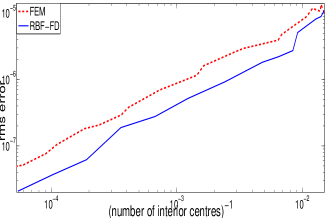
(a) $\omega=\pi+0.01$: errors on centers

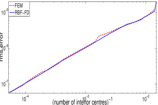
(b) $\omega=\pi+0.01$: errors on grid

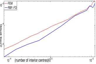
(c) $\omega=5\pi/4$: errors on centers

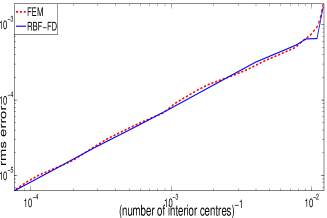
(d) $\omega=5\pi/4$: errors on grid

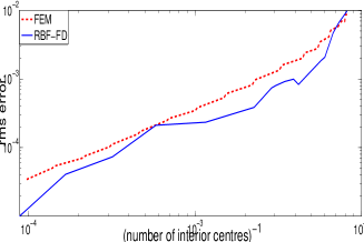
(e) $\omega=7\pi/4$: errors on centers

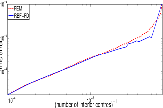
(f) $\omega=7\pi/4$: errors on grid

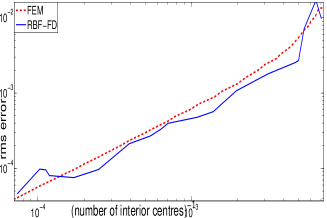
(g) $\omega=2\pi$: errors on centers

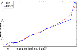
(h) $\omega=2\pi$: errors on grid

Figure 7: Test Problem 3: Errors for various values of $\omega$ on the centers (left) and on a grid (right). RBF-FD: the method of this paper, FEM: finite element method with piecewise linear shape functions, where the solution is computed by using MATLAB PDE Toolbox with default parameters of the adaptive refinement.

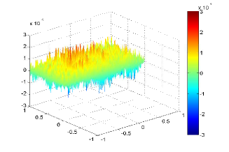
(a) $\omega=\pi+0.01$: RBF-FD

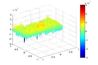
(b) $\omega=\pi+0.01$: FEM

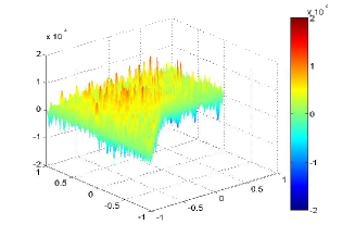
(c) $\omega=5\pi/4$: RBF-FD

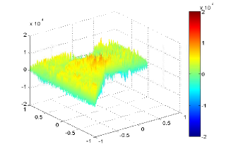
(d) $\omega=5\pi/4$: FEM

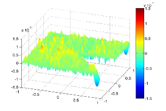
(e) $\omega=7\pi/4$: RBF-FD

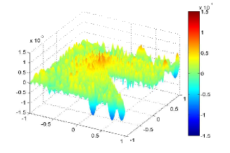
(f) $\omega=7\pi/4$: FEM

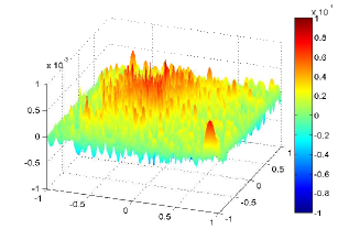
(g) $\omega=2\pi$: RBF-FD

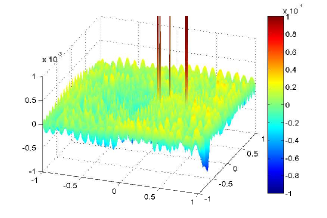
(h) $\omega=2\pi$: FEM

Figure 8: Test Problem 3: Error functions for RBF-FD (left) and FEM (right). The number of interior centers/vertices: (a) 2786, (b) 2768, (c) 3592, (d) 3478, (e) 1721, (f) 1427, (g) 2553, (h) 2521. These centers and vertices are shown in Figure 9.

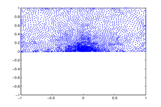
(a) $\omega=\pi+0.01$: RBF-FD

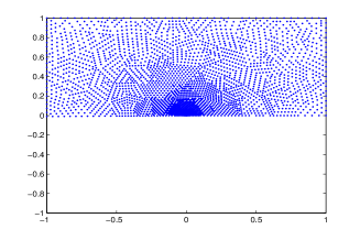
(b) $\omega=\pi+0.01$: FEM

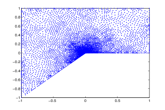
(c) $\omega=5\pi/4$: RBF-FD

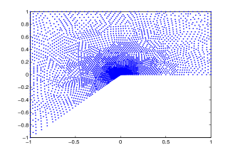
(d) $\omega=5\pi/4$: FEM

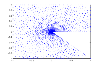
(e) $\omega=7\pi/4$: RBF-FD

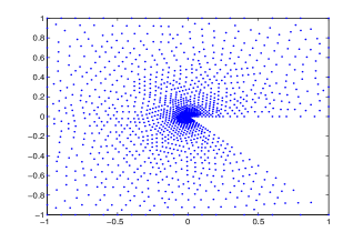
(f) $\omega=7\pi/4$: FEM

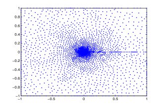
(g) $\omega=2\pi$: RBF-FD

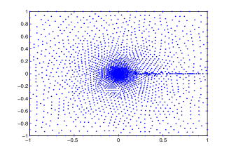
(h) $\omega=2\pi$: FEM

Figure 9: Test Problems 3: Centers generated by the adaptive RBF-FD method (left) and the vertices of the triangulations generated by the adaptive FEM (right) for the solutions whose error plots are shown in Figure 8.

Test Problem 4.

(Curved Slit) Dirichlet problem for the Laplace equation $\Delta u=0$ in the domain $\Omega$ obtained from $(-1,1)^{2}$ by removing the arc of the circle with center at $(1,-0.75)$ and radius $1.25$ between the points $(0,0)$ and $(1,0.5)$. The boundary conditions are chosen such that the exact solution is $u(x,y)=\operatorname{Re}\sqrt{(3-4i)z/(z-2)}$, with $z=x+iy$.

The domain and the exact solution $u$ are illustrated in Figure 10. The exact solution behaves as $r^{1/2}$ at the origin, that is the strength of the singularity is the same as for the slit domain of Test Problem 3 with $\omega=2\pi$. The numerical results are presented in Figure 11 and are similar to the results for Test Problem 3 with $\omega=2\pi$, which shows that the curvature of the slit does not present any significant additional challenge.

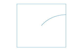
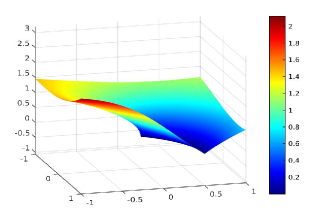
Figure 10: Test Problem 4: Domain with a curved slit (left) and exact solution (right).

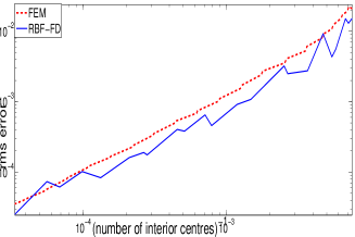
(a) Errors on centers

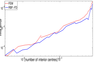
(b) Errors on grid

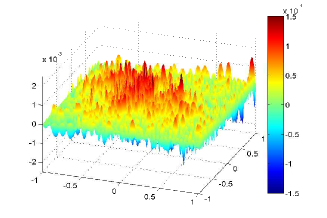
(c) RBF-FD error (2204)

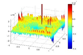
(d) FEM error (2236)

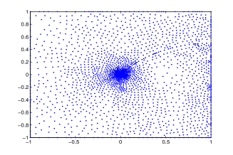
(e) RBF-FD centers (2204)

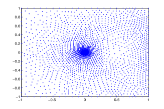
(f) FEM centers (2236)

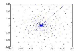
(g) RBF-FD centers: zoom

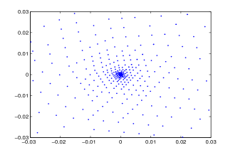
(h) FEM centers: zoom

Figure 11: Test Problem 4: Errors and centers as in Figure 4. The plots in (cd) are based on the RBF-FD solution on 2204 interior centers shown in (e) and the FEM solution on 2236 interior vertices shown in (f).

Test Problem 5.

[8, Section 2.8: Oscillatory] Dirichlet problem (1) for the Helmholtz equation $-\Delta u-\frac{1}{(\alpha+r)^{4}}u=f$, $r=\sqrt{x^{2}+y^{2}}$, in the domain $\Omega=(0,1)^{2}$, where the right hand side and the boundary conditions are chosen such that the exact solution $u$ is $\sin(\frac{1}{\alpha+r})$, with $\alpha=\frac{1}{10\pi}$ or $\frac{1}{50\pi}$.

The solutions for both $\alpha=\frac{1}{10\pi}$ and $\frac{1}{50\pi}$ are highly oscillatory near the origin, with increasing frequency closer to the origin, see Figure 12.

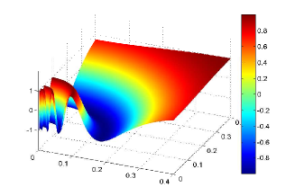
(a) $\alpha=\frac{1}{10\pi}$

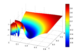
(b) $\alpha=\frac{1}{50\pi}$

Figure 12: Test Problem 5: Exact solutions for $\alpha=\frac{1}{10\pi}$ and $\frac{1}{50\pi}$.

Numerical results for Test Problem 5 with $\alpha=\frac{1}{10\pi}$ are presented in Figure 13. We see that RBF-FD is generally more accurate than FEM in this case. Moreover, Figures (e) and (f) suggest that the RBF-FD solution is less susceptible to a bias in the areas of high oscillation, manifested in a systematic underestimation of the amplitude of the oscillations. Figure (g) shows that the centers produced by the RBF-FD method reproduce to some extent the distinctive ring-like pattern seen in the FEM vertices of (h). This pattern is easy to explain by comparing Figures 13(gh) with Figure 14(a) which shows a color-mapped image of the exact solution in the same area. The centers are placed more densely in the highly curved regions at the tops and bottoms of the waves and neglect the rather flat regions between them. This placement of the centers is known to be advantageous for piecewise linear approximation and other approximation methods with leading error term related to the size of the second order derivatives or the curvature of the exact solution [1]. This test has been the main motivation for us to replace the error indication $\varepsilon_{0}(\zeta,\xi)$ by $\varepsilon_{1}(\zeta,\xi)$ as explained in Section 3. If we apply RBF-FD method of this paper with $\varepsilon_{0}$ instead of $\varepsilon_{1}$, then we get the rings of centers with high density shifted to the flat regions of high gradient as illustrated in Figure 14(b). As a result, as naturally expected, the overall error is much larger and the accuracy is particularly poor near the tops and bottoms of waves, see Figure 14(cd).

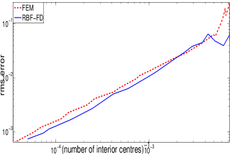
(a) Errors on centers

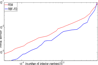
(b) Errors on grid

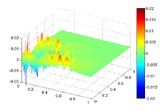
(c) RBF-FD error

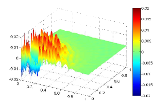
(d) FEM error

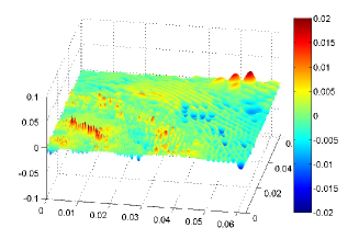
(e) RBF-FD error: zoom

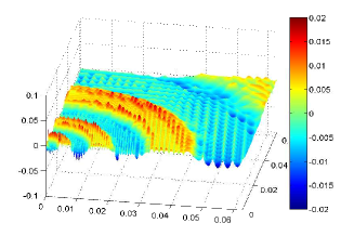
(f) FEM error: zoom

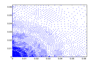
(g) RBF-FD centers: zoom

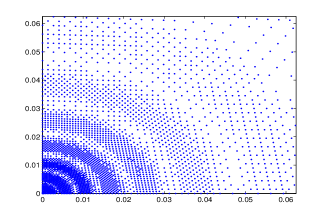
(h) FEM centers: zoom

Figure 13: Test Problem 5 with $\alpha=\frac{1}{10\pi}$: Errors and centers/vertices. The plots in (ceg) are based on the RBF-FD solution with 4029 interior centers, whereas those in (dfh) on the FEM solution with 3806 interior vertices.

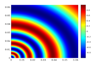
(a) Zoom of the exact solution

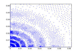
(b) Centers with error indicator $\varepsilon_{0}$

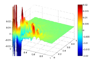
(c) Error graph

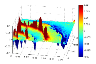
(d) Error graph: zoom

Figure 14: Test Problem 5 with $\alpha=\frac{1}{10\pi}$: (a) Exact solution in the subregion used in Figure 13(e-h) and in (bd) of this figure. (b-d) Centers and errors for the solution with 3679 interior centers obtained by RBF-FD method with error indicator $\varepsilon_{0}(\zeta,\xi)=|\hat{u}_{\zeta}-\hat{u}_{\xi}|$.

Figure 15 illustrates the results for Test Problem 5 with $\alpha=\frac{1}{50\pi}$. The layout is the same as in Figure 13, and the results are similar. There is no ring-like pattern in the locations of the centers in (g) because the solution is relatively less resolved than the one in Figure 13(g). Indeed, in Figures 15(gh) we see about 5 centers across the waves near the origin versus 12 or more in Figures 13(gh).

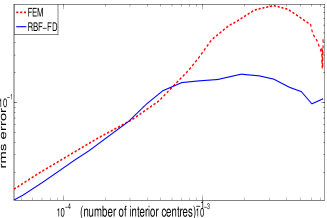
(a) Errors on centers

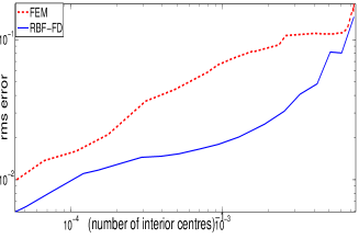
(b) Errors on grid

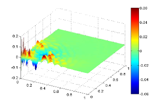
(c) RBF-FD error

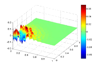
(d) FEM error

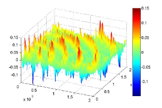
(e) RBF-FD error: zoom

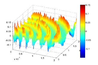
(f) FEM error: zoom

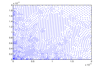
(g) RBF-FD centers: zoom

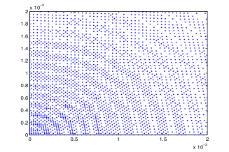
(h) FEM centers: zoom

Figure 15: Test Problem 5 with $\alpha=\frac{1}{50\pi}$: Errors and centers/vertices. The plots in (ceg) are based on the RBF-FD solution with 13964 interior centers, whereas those in (dfh) on the FEM solution with 14942 interior vertices.

Test Problem 6.

[8, Section 2.4: Peak] Dirichlet problem (1) for the Poisson equation $\Delta u=f$ in the domain $\Omega=(0,1)^{2}$, where the right hand side $f$ and the boundary conditions are chosen such that the exact solution is $u(x)=e^{-\alpha\|x-x_{0}\|^{2}}$. Following [8], two instances of this problem, with the following values of the parameters $\alpha$ (the strength of the peak) and $x_{0}$ (the location of the peak) will be considered:

• $\alpha=1000$, $x_{0}=(0.5,0.5)$,

• $\alpha=100000$, $x_{0}=(0.51,0.117)$.

The exact solutions are presented in Figure 16, and the error curves in Figure 17. In contrast to the previous test problems there is a significant difference in the behavior of the FEM and RBF-FD methods. The errors of the RBF-FD method are smaller on denser sets of centers, but higher for a number of initial refinements. Therefore we also computed RBF-FD solutions on the centers/vertices generated by the adaptive finite element method and included the respective curves in the same figure. The errors in this case are much closer to those by the FEM. In addition, in the case (a) we also produced smoothly distributed centers using distmesh2d, which gives results closer to those by the FEM as well. We again used different values for the initial edge length $h_{0}$ and the edge length function in the form $\sigma(r)=r^{\beta}$ to obtain sets with different numbers of centers, and picked the constellations of $h_{0},\beta$ shown in Table 2 which produce results with relatively small errors of the RBF-FD method.

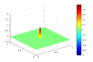
(a)   

(b)  

Figure 16: Exact solutions for both versions of Test Problem 6.

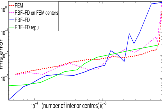
(a) Errors on centers for 5(a)

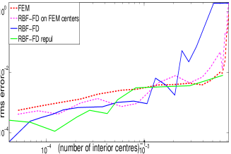
(b) Errors on grid for 5(a)

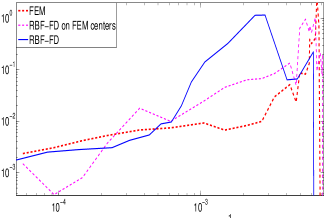
(c) Errors on centers for 5(b)

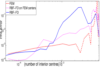
(d) Errors on grid for 5(b)

Figure 17: Test Problem 6: Errors with $\alpha=1000$, $x_{0}=(0.5,0.5)$ (top) and $\alpha=100000$, $x_{0}=(0.51,0.117)$ (bottom). RBF-FD: the method of this paper, FEM: finite element method with piecewise linear shape functions, RBF-FD on FEM centers: RBF-FD method with stencil support selection by Algorithm 1 on centers generated by the adaptive finite element method, RBF-FD repul: RBF-FD method with stencil support selection by Algorithm 1 on centers generated by a priori refinement using DistMesh.

$\#\Xi_{\rm int}$	157	343	1216	1863	2375	3600	4850	8150	14411	24191
$h_{0}$	.00036	.001	.00055	.000325	.00045	.0006	.00045	.00035	.00045	.0005
$\beta$	0.675	0.65	0.525	0.575	0.525	0.475	0.475	0.475	0.4	0.375

Table 2: Parameters of distmesh2d.m used to produce the a priori sets of centers for Test Problem 6 with $\alpha=1000$, $x_{0}=(0.5,0.5)$: $\#\Xi_{\rm int}$ is the number of interior centers, $h_{0}$ the initial edge length, and $\beta$ the power of the scaled edge length function in the form $\sigma(r)=r^{\beta}$. The sets with $\#\Xi_{\rm int}=343$ and 1863 are illustrated in Figure 20.

Some solutions of Test Problem 6 with $\alpha=1000$, $x_{0}=(0.5,0.5)$ by FEM and the three versions of RBF-FD are illustrated in Figure 18, whereas the centers produced by all methods can be seen in Figures 19 and 20. Figures 18(a-d) compare solutions for a small number of interior centers/vertices of about 350. We can see in particular that although the adaptive RBF-FD solution is visually different from the exact solution in Figure 16(a), it does have the shape of a peak in the correct location. Figures 18(e-h) compare the errors of the solutions with about 1700–1900 interior centers/vertices. In this case the RBF-FD-based solutions are more accurate than the FEM solution. Furthermore, Figure 19 compares adaptively generated centers in the RBF-FD method using Algorithms 1 and 2 with the distribution of the vertices of the triangulations used by the FEM. In particular, the plots in Figure 19(ab) explain the difference in the solutions shown in Figures 18(ab) as they indicate much higher concentration of the FEM vertices near the peak in comparison to the RBF-FD centers. Note that 350 interior RBF-FD centers are obtained after just 3 refinements, whereas 343 interior vertices of FEM are generated after 8 refinement steps of the same initial set of centers. If we compute an RBF-FD solution using Algorithm 1 on the FEM centers shown in Figure 19(b), then the result is very close to the FEM solution, see Figure 18(c) and the corresponding points on the curves in Figure 17(ab). The RBF-FD solution using Algorithm 1 on the smoothly distributed centers shown in Figure 20(a) are also close to the FEM solution, see Figure 18(d). The appropriately zoomed sets of centers/vertices shown in Figures 19(c-h) demonstrate that RBF-FD centers on further refinements are distributed similar to the FEM vertices. Note that the smoothly distributed centers in Figure 20 do not exhibit the same abrupt change in the density as seen in Figure 19 for the adaptive methods. Nevertheless, the error of RBF-FD solutions on these centers is small as well, see Figures 17(ab) and 18(h).

(a) FEM solution (343)

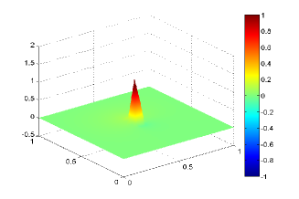
(b) RBF-FD solution (350)

(c) RBF-FD on FEM centers (343)

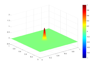
(d) RBF-FD on smooth centers (343)

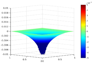
(e) FEM error (1699)

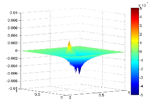
(f) RBF-FD error (1893)

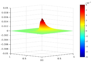
(g) RBF-FD on FEM centers (1699)

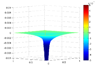
(h) RBF-FD on smooth centers (1863)

Figure 18: Test Problem 6 with $\alpha=1000$ and $x_{0}=(0.5,0.5)$: (a) FEM solution for a triangulation with 343 interior vertices, (b) RBF-FD solution for 350 interior centers, (c) RBF-FD solution with stencil support selection by Algorithm 1 on centers at the 343 interior vertices of FEM triangulation, (d) RBF-FD solution with stencil support selection by Algorithm 1 on centers generated by a priori refinement using DistMesh, (e-h) error plots for the FEM solution for a triangulation with 1699 interior vertices and three versions of RBF-FD as above, with the number of interior vertices given in brackets.

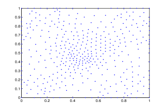
(a) RBF-FD centers (350)

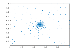
(b) FEM centers (343)

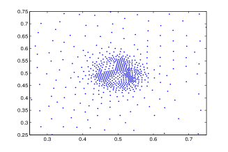
(c) RBF-FD centers (765)

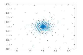
(d) FEM centers (718)

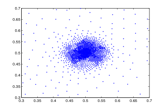
(e) RBF-FD centers (1893)

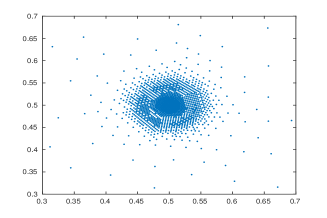
(f) FEM centers (1699)

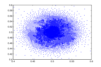
(g) RBF centers (6689)

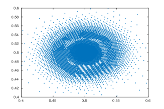
(h) FEM centers (7520)

Figure 19: Test Problem 6 with $\alpha=1000$ and $x_{0}=(0.5,0.5)$: Centers for RBF-FD and FEM adaptive refinements. The number of interior centers/vertices is shown in brackets. The number of refinements of an initial set of centers: (a) 3, (b) 8, (c) 7, (d) 10, (e) 10, (f) 14, (g) 13, (h) 15.

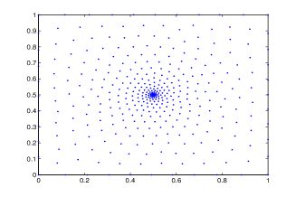
(a) Repulsion centers (343)

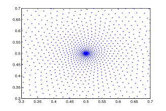
(b) Repulsion centers (1863)

Figure 20: Test Problem 6 with $\alpha=1000$ and $x_{0}=(0.5,0.5)$: Centers generated by a priori refinement using DistMesh with (a) $h_{0}=0.001$, $\beta=0.65$ and (a) $h_{0}=0.000325$, $\beta=0.575$.

Finally, Table 3 includes the data on the uniformity measures $v_{\mathrm{max}},v_{\mathrm{aver}},c_{\mathrm{max}},c_{\mathrm{aver}}$ defined at the end of Section 2 for the stencil supports obtained in the experiments for each test problem solved by the RBF-FD method. We see that the value of $v_{\mathrm{aver}}$ is around 2.0 for the adaptively generated centers, which means that for most stencils the angle uniformity quotient $\overline{\alpha}/\underline{\alpha}$ is significantly less than the tolerance $v=2.5$ used in the termination criterion of Step II.2.ii.b. Nevertheless, there are always stencils with $\overline{\alpha}/\underline{\alpha}$ reaching about 4.0 and in some cases up to 7.0, which means that the termination happens at Step II.1 in order to prevent a very high non-uniformity of distances. The average of the distance uniformity quotient (8) is also very stable at around 1.3, and typical maximum values are about 2.5. This shows altogether that the majority of the stencil supports produced by the adaptive RBF-FD method of this paper are remarkably well-balanced geometrically. In the experiments with smoothly distributed a priori centers generated by DistMesh (see the rows of the table marked 1s and 6as) the numbers are significantly smaller, which is expected.

TP	$v_{\mathrm{max}}$	$v_{\mathrm{aver}}$	$c_{\mathrm{max}}$	$c_{\mathrm{aver}}$
1	3.93	2.02	2.45	1.30
1s	2.71	1.40	2.17	1.11
2	3.82	2.01	2.43	1.29
3a	4.22	2.02	2.38	1.29
3b	3.98	2.02	2.52	1.30
3c	5.01	2.02	2.39	1.31
3d	6.97	2.02	2.52	1.31
4	7.00	2.02	2.46	1.30
5a	5.22	2.02	2.69	1.29
5b	4.98	2.02	2.47	1.28
6a	4.29	2.00	2.41	1.28
6as	2.85	1.39	2.24	1.11
6b	4.39	2.00	2.46	1.28

Table 3: The uniformity measures $v_{\mathrm{max}},v_{\mathrm{aver}},c_{\mathrm{max}},c_{\mathrm{aver}}$ (defined at the end of Section 2) for the stencil supports obtained in each test problem. The column marked ‘TP’ contains the test problem number and optional letters. 1s: Test Problem 1 with smoothly distributed centers of DistMesh. 3a, 3b, 3c, 3d: Test Problem 3 with $\omega=\pi+0.01$, $5\pi/4$, $7\pi/4$ and $2\pi$, respectively. 5a, 5b: Test Problem 5 with $\alpha=\frac{1}{10\pi}$ and $\frac{1}{50\pi}$, respectively. 6a, 6b: versions (a) and (b) of Test Problem 6. 6as: version (a) of Test Problem 6 with smoothly distributed centers of DistMesh.

5 Conclusion

In this paper we suggested an adaptive meshless RBF-FD method for the numerical solution of elliptic problems with point singularities. Both ingredients of the method, Algorithm 1 for stencil support selection and Algorithm 2 for adaptive refinement have been tested on several benchmark problems with different types of point singularities, including the problems of this type suggested in [8] for testing adaptive refinement methods. The numerical results show that the method generates reasonably distributed adaptive centers similar to the distribution of the centers/vertices from the mesh-based adaptive finite element method, and the errors are nearly equidistributed. For Test Problems 1–5 the size of the error is close to that of the FEM approximation from the same number of centers. For Test Problem 6 whose solution features an exponential peak in the interior of the domain, the refinement regime of our method significantly differs from that of the adaptive finite element method used for comparison, which results in a higher accuracy on fine sets of centers at the expense of a lower accuracy on the initial coarse refinements. When finite element centers are used instead of those generated by Algorithm 2, the errors are in a close agreement with the errors of the FEM method.

The method of this paper significantly improves our earlier adaptive meshless RBF-FD method introduced in [3] which suffered from certain deterioration of the quality of the centers after a number of successive refinements. This undesirable behavior has disappeared, and this has not even happened at the expense of the efficiency, which has in fact also improved because we were able to remove a post-processing step in the predecessor of Algorithm 2 in [3] whose goal was to reduce the deterioration. A single most important new feature of Algorithm 2 is an error indicator of Zienkiewicz-Zhu type used instead of a simple gradient estimate employed in [3]. This leads to a significant improvement of the results for Test Problem 4 with a highly oscillatory solution, as demonstrated in the error plots of Figures 13 and 14. The new stencil support selection algorithm (Algorithm 1) produces geometrically better well-balanced stencils thanks to the introduction of a second termination criterion (7).

We expect that adaptive algorithms may be further improved by developing more sophisticated error indicators. Further research is needed in order to achieve a similar competitive performance of meshless RBF-FD methods for problems with line or curve singularities, boundary layers and wave fronts, as well as for time depending problems with evolving singularities.

References

- [1] M. S. Birman and M. Z. Solomyak. Piecewise-polynomial approximations of functions of the classes . Mathematics of the USSR-Sbornik, 2(3):295, 1967.
- [2] Martin D. Buhmann. Radial Basis Functions. Cambridge University Press, New York, NY, USA, 2003.
- [3] Oleg Davydov and Dang Thi Oanh. Adaptive meshless centres and RBF stencils for Poisson equation. Journal of Computational Physics, 230:287–304, 2011.
- [4] Oleg Davydov and Dang Thi Oanh. On the optimal shape parameter for Gaussian radial basis function finite difference approximation of the Poisson equation. Computers and Mathematics with Applications, 62:2143–2161, 2011.
- [5] Oleg Davydov and Robert Schaback. Error bounds for kernel-based numerical differentiation. Numerische Mathematik, 132:243–269, 2016.
- [6] Bengt Fornberg and Natasha Flyer. A Primer on Radial Basis Functions with Applications to the Geosciences. SIAM, Philadelphia, 2015.
- [7] Bengt Fornberg, Erik Lehto, and Collin Powell. Stable calculation of Gaussian-based RBF-FD stencils. Computers and Mathematics with Applications, 65(4):627 – 637, 2013.
- [8] William F. Mitchell. A collection of 2D elliptic problems for testing adaptive grid refinement algorithms. Applied Mathematics and Computation, 220:350 – 364, 2013.
- [9] Vinh Phu Nguyen, Timon Rabczuk, Stéphane Bordas, and Marc Duflot. Meshless methods: A review and computer implementation aspects. Mathematics and Computers in Simulation, 79(3):763–813, 2008.
- [10] Areti Papastavrou and Rüdiger Verfürth. A posteriori error estimators for stationary convection-diffusion problems: a computational comparison. Computer Methods in Applied Mechanics and Engineering, 189(2):449 – 462, 2000.
- [11] Partial Differential Equation Toolbox™ User’s Guide. The MathWorks, Inc, 2009.
- [12] Per-Olof Persson and Gilbert Strang. A simple mesh generator in matlab. SIAM Review, 46(2):329–345, 2004.
- [13] Lars B. Wahlbin. Local behavior in finite element methods. In Finite Element Methods (Part 1), volume 2 of Handbook of Numerical Analysis, pages 353 – 522. Elsevier, 1991.
- [14] O. C. Zienkiewicz and J. Z. Zhu. A simple error estimator and adaptive procedure for practical engineering analysis. International Journal for Numerical Methods in Engineering, 24(2):337–357, 1987.