Inverse Construction of the $\Lambda$LTB Model
from a Distance-redshift Relation

Abstract

Spherically symmetric dust universe models with a positive cosmological constant $\Lambda$, known as $\Lambda$-Lemaître-Tolman-Bondi($\Lambda$LTB) models, are considered. We report a method to construct the $\Lambda$LTB model from a given distance-redshift relation observed at the symmetry center. The spherical inhomogeneity is assumed to be composed of growing modes. We derive a set of ordinary differential equations for three functions of the redshift, which specify the spherical inhomogeneity. Once a distance-redshift relation is given, with careful treatment of possible singular points, we can uniquely determine the model by solving the differential equations for each value of $\Lambda$. As a demonstration, we fix the distance-redshift relation as that of the flat $\Lambda$CDM model with $(\Omega^{\rm dis}_{\rm m0},\Omega^{\rm dis}_{\rm\Lambda 0})=(0.3,0.7)$, where $\Omega^{\rm dis}_{\rm m0}$ and $\Omega^{\rm dis}_{\rm\Lambda 0}$ are the normalized matter density and the cosmological constant, respectively. Then, we construct the $\Lambda$LTB model for several values of $\Omega_{\rm\Lambda 0}:=\Lambda/(3H_{0}^{2})$, where $H_{0}$ is the present Hubble parameter observed at the symmetry center. We obtain void structure around the symmetry center for $\Omega_{\Lambda 0}<\Omega^{\rm dis}_{\Lambda 0}$. We show the relation between the ratio $\Omega_{\Lambda 0}/\Omega^{\rm dis}_{\Lambda 0}$ and the amplitude of the inhomogeneity.

I Introduction

The cosmological principle is one of the most fundamental principles in cosmology, and established as a useful and successful working hypothesis. However, it is still of interest to consider the largest amplitude of cosmological scale inhomogeneity which can be compatible with the latest observational data. In other words, observational tests of the cosmological principle with precision measurements may be interesting subjects in observational cosmology. Since the isotropy of our universe is strongly supported by the isotropy of the cosmic microwave background(CMB), in this paper, we focus on spherically symmetric universe models with an observer at the symmetry center.

Spherically symmetric inhomogeneous universe models have attracted much attention as alternative models to explain the apparent accelerated expansion of our universe without a cosmological constantZehavi:1998gz ; Celerier:1999hp ; Tomita:1999qn . After the compatibility with the CMB anisotropy was discussed in Ref. Alnes:2005rw , many observational constraints on the spherical inhomogeneity were discussed by using Type Ia supernovae data, CMB anisotropy, baryon acoustic oscillation and so on(see, e.g. Ref. Redlich:2014gga for a recent detailed analysis). Those analyses, especially constraints from the kinematic Sunyaev-Zeldovich effectGarciaBellido:2008gd , revealed that the apparent accelerated expansion cannot be explained only by introducing spherical inhomogeneity without a cosmological constant if we assume the standard history of our universe before the photon last scattering. If we do not assume the inflationary paradigm and the standard thermal history before the photon last scattering, the model significantly loses its predictability and comparable observations. However, even such eccentric models would be tested by future precision observations of the late time expansion of our universeUzan:2008qp ; Yoo:2008su ; Quartin:2009xr ; Yoo:2010hi ; Yagi:2011bt .

In this paper, we consider spherically symmetric dust universe models with a positive cosmological constant $\Lambda$, known as $\Lambda$-Lemaître-Tolman-Bondi($\Lambda$LTB) models. When we consider the relation between spherical inhomogeneity in $\Lambda$LTB models and observables, one of useful strategies is the inverse construction of the model inhomogeneity starting from given observables. A pioneering work has been done by Mustapha, Hellaby and Ellis in Ref. Mustapha:1998jb , where the angular diameter distance and the redshift-space mass density were supposed as the observables. The approach proposed in Ref. Mustapha:1998jb has been successfully performed in Refs. Lu:2007gr ; McClure:2007hy ; Celerier:2009sv ; Kolb:2009hn ; Dunsby:2010ts for specific situations. Another important approach was proposed by Iguchi, Nakamura and Nakao(INN)Iguchi:2001sq , where the inhomogeneity is assumed to be composed of growing modes. This assumption is often adopted to guarantee the compatibility with the inflationary paradigm. The INN approach has been solved in Ref. Yoo:2008su in the whole redshift range. Apart from these two approaches, there are also several related works on the inverse constructionCelerier:1999hp ; Chung:2006xh ; Vanderveld:2006rb ; Romano:2009mr ; Romano:2009ej ; Krasinski:2014yja ; Romano:2013bxa .

In this paper, along the INN approach, we explicitly construct the $\Lambda$LTB models whose distance-redshift relation coincides with that in the flat $\Lambda$CDM model with $(\Omega^{\rm dis}_{\rm m0},\Omega^{\rm dis}_{\rm\Lambda 0})=(0.3,0.7)$, where $\Omega^{\rm dis}_{\rm m0}$ and $\Omega^{\rm dis}_{\rm\Lambda 0}$ are the normalized matter density and the cosmological constant for the flat $\Lambda$CDM model, respectively. It should be noted that $\Omega^{\rm dis}_{\rm m0}$ and $\Omega^{\rm dis}_{\rm\Lambda 0}$ are the parameters characterizing the distance-redshift relation, and $\Omega^{\rm dis}_{\rm\Lambda 0}$ is not necessarily equal to $\Omega_{\Lambda 0}:=\Lambda/(3H_{0}^{2})$, where $H_{0}$ is the present Hubble parameter observed at the symmetry center. Since we add a parameter $\Lambda$ to the case in the preceding worksIguchi:2001sq ; Yoo:2008su ; Yoo:2010qn , we obtain an one-parameter family of solutions for a given set of values $(\Omega^{\rm dis}_{\rm m0},\Omega^{\rm dis}_{\rm\Lambda 0})$. The one-parameter family can be characterized by the parameter $\Omega_{\Lambda 0}$. The difference between $\Omega_{\Lambda 0}$ and $\Omega^{\rm dis}_{\Lambda 0}$ can be regarded as a systematic error in estimation of $\Lambda$ due to the spherical inhomogeneity as is discussed in Refs. Romano:2011mx ; Negishi:2015oga . In order to estimate the magnitude of the systematic error due to possible inhomogeneity, we calculate the amplitude of the inhomogeneity for several values of $\Omega_{\Lambda 0}/\Omega^{\rm dis}_{\Lambda 0}$. The method used in this paper is similar to that in Appendix of Ref. Yoo:2010qn , where a cosmological constant is not considered and the LTB solution can be described by a simple parametric form. In this paper, we work through all the complexity associated with a positive finite value of the cosmological constant(see Ref. Valkenburg:2011tm for fast accurate evaluation of metric components). Similar analysis has been done in Ref. Negishi:2015oga for perturbations on a homogeneous background.

In this paper, we use the geometrized units in which the speed of light and Newton’s gravitational constant are one, respectively.

II Conditions to determine the $\Lambda$LTB model

II.1 $\Lambda$LTB model and the radial geodesic

We consider the $\Lambda$-Lemaître-Tolman-Bondi ($\Lambda$LTB) solution, whose line element is given by

$$\mathrm{d}s^{2}=-\mathrm{d}t^{2}+\frac{(\partial_{r}R(t,r))^{2}}{1-k(r)r^{2}}\mathrm{d}r^{2}+R^{2}(t,r)\mathrm{d}\Omega^{2},$$ (1)

where $k(r)$ is an arbitrary function of $r$ and $R(t,r)$ is the areal radius. The energy-momentum tensor is given by that of dust fluids:

$$T^{\mu\nu}=\rho(t,r)u^{\mu}u^{\nu},$$ (2)

where $\rho(t,r)$ is the mass density and $u^{\mu}$ is the 4-velocity of dust particles. From the Einstein equations, we obtain the following equation:

$$(\partial_{t}R)^{2}=-k(r)r^{2}+\frac{2M(r)}{R}+\frac{1}{3}\Lambda R^{2},$$ (3)

where $M(r)$ is an arbitrary function of $r$. By using $M(r)$, we can write $\rho(t,r)$ as follows:

$$\rho(t,r)=\frac{1}{4\pi}\frac{\partial_{r}M(r)}{R^{2}\partial_{r}R}.$$ (4)

For convenience, we introduce the following functions:

$$m(r):=\frac{6M(r)}{r^{3}}\quad,\quad S(t,r):=\frac{R(t,r)}{r}.$$ (5)

Then, Eq. (3) is written as follows:

$$(\partial_{t}S)^{2}=f(r,S):=-k(r)+\frac{m(r)}{3S}+\frac{1}{3}\Lambda S^{2}.$$ (6)

Eq. (6) can be integrated as

$$t-t_{B}(r)=\int_{0}^{S}\frac{dX}{\sqrt{f(r,X)}}$$ (7)

with an arbitrary function $t_{B}(r)$, which is called the bang time function because the areal radius $R$ vanishes at $t=t_{B}(r)$. When we consider the case $k(r)=$const. and $m(r)=$const., small perturbative inhomogeneity associated with $t_{\rm B}(r)$ is given by purely decaying modes in terms of cosmological perturbation theory. Therefore, in this paper, we simply assume that the bang time function is constant to guarantee the compatibility with the inflationary paradigm. The constant value of $t_{\rm B}$ can be eliminated by the time shift degree of freedom, namely, we can set $t_{B}(r)=0$.

We assume that the observer is at the symmetry center $r=0$. Then, we consider the past light-cone emanated from the symmetry center expressed by a trajectory parametrized by the redshift as follows:

$$t=t_{\rm lc}(z),$$ (8)

$$r=r_{\rm lc}(z).$$ (9)

Hereafter, for notational simplicity, we often omit the subscript “lc”. The null geodesic equations in the $\Lambda$LTB solution is given as

$$\frac{\mathrm{d}r}{\mathrm{d}z} = \frac{1}{1+z}\frac{\sqrt{1-kr^{2}}}{\sqrt{f}+r\partial_{t}\partial_{r}S},$$ (10)

$$\frac{\mathrm{d}t}{\mathrm{d}z} = -\frac{1}{1+z}\frac{S+r\partial_{r}S}{\sqrt{f}+r\partial_{t}\partial_{r}S}.$$ (11)

II.2 Conditions to determine the arbitrary functions

The $\Lambda$LTB solution has three arbitrary functions $k(r)$, $m(r)$ and $t_{B}(r)$. One of these functional degrees of freedom corresponds to the gauge degree of freedom associated with the choice of the radial coordinate $r$. We impose a gauge condition for the radial coordinate $r$ and require the distance-redshift relation coincides with a given function $D_{\rm A}(z)$.

We fix the gauge by imposing the light-cone gauge condition given by

$$t(z)=t_{0}-r(z),$$ (12)

where $t_{0}$ is the present time at the central observer. From this condition, $t_{\rm lc}$ can be trivially given by $r_{\rm lc}$. Therefore, the remaining independent functions are $r_{\rm lc}(z)$, $k(r_{\rm lc}(z))$ and $m(r_{\rm lc}(z))$. Combining the light-cone gauge condition and the geodesic equations, we obtain

$$\left.\left(r\partial_{r}S+S-\sqrt{1-kr^{2}}\right)\right|_{r=r_{\rm lc},~{}t=t_{\rm lc}}=0.$$ (13)

We consider Eqs. (10), (11) and (13) as independent equations.

The angular diameter distance on the past light-cone is given by $R(t(z),r(z))$. We impose that the angular diameter distance coincides with a given function $D_{\rm A}(z)$. In practice, we impose the following differential equation:

$$\frac{\mathrm{d}R}{\mathrm{d}z}=\frac{\mathrm{d}D_{A}}{\mathrm{d}z}.$$ (14)

In this paper, for demonstration, we use the distance-redshift relation in a flat $\Lambda$CDM universe instead of actual observational data. That is, we use the distance characterized by the cosmological parameters for the flat $\Lambda$CDM universe as follows:

$$D_{A}(z)=D_{\rm\Lambda CDM}(z;\Omega_{\rm m0}^{\rm{dis}},\Omega_{\Lambda 0}^{\rm{dis}}),$$ (15)

where $\Omega_{\rm m0}^{\rm{dis}}$ and $\Omega_{\Lambda 0}^{\rm{dis}}$ are the normalized matter density and the cosmological constant for the flat $\Lambda$CDM model. It should be noted that in a spherically symmetric inhomogeneous universe model, the Hubble parameter cannot be uniquely determined in off-center regions because of the difference between the radial direction and the transverse direction. The Hubble parameter can be uniquely defined only at the symmetry center. We define the present Hubble parameter $H_{0}$ as follows:

$$H_{0}:=\left(\partial_{t}R/R\right)_{z=0}.$$ (16)

The normalization of the cosmological parameters, e.g. $\Omega_{\rm m0}^{\rm{dis}}$, is performed by using $H_{0}$. In our numerical calculations, we use the unit system given by $H_{0}=1$, and all dimensionful variables are normalized by $H_{0}$.

III Derivation of differential equations

Let us derive the differential equations to determine three arbitrary functions $r(z)$, $k(z)$ and $m(z)$. Differentiating Eq. (3) with respect to $r$, we obtain

$$\partial_{t}\partial_{r}S = \frac{1}{2}f^{-1/2}$$ (18)

$$\times\left(-\partial_{r}k+\frac{S\partial_{r}m-m\partial_{r}S}{3S^{2}}+\frac{2}{3}\Lambda S\partial_{r}S\right).~{}~{}~{}~{}~{}$$

Multiplying $\mathrm{d}r/\mathrm{d}z$ to the above equation and using the null geodesic equations (10) and (11), we get the following differential equation:

$$\biggr{[}\biggr{(}-\frac{m}{3S^{2}}+\frac{2}{3}\Lambda S\biggr{)}\biggr{(}\sqrt{1-kr^{2}}-S\biggr{)}+2f\biggr{]}\frac{\mathrm{d}r}{\mathrm{d}z}$$ (19)

$$-r\frac{\mathrm{d}k}{\mathrm{d}z}+\frac{r}{3S}\frac{\mathrm{d}m}{\mathrm{d}z}-\frac{2\sqrt{f}\sqrt{1-kr^{2}}}{1+z}=0.$$ (20)

Differentiating Eq. (7) with respect to $r$, we obtain

$$0 = \frac{\partial_{r}S}{\sqrt{f(r,S)}}$$ (22)

$$-\frac{1}{2}\int_{0}^{S}f(r,X)^{-2/3}\left(-\partial_{r}k+\frac{\partial_{r}m}{3X}\right)\mathrm{d}X.~{}~{}$$

Multiplying $\mathrm{d}r/\mathrm{d}z$ to the above equation and using Eq. (13), we get the following differential equation:

$$0=\frac{\sqrt{1-kr^{2}}-S}{r\sqrt{f}}\frac{\mathrm{d}r}{\mathrm{d}z}-P\frac{\mathrm{d}k}{\mathrm{d}z}+\frac{Q}{3}\frac{\mathrm{d}m}{\mathrm{d}z},$$ (23)

where

$$P:=-\frac{1}{2}\int_{0}^{S}f(r,X)^{-3/2}\mathrm{d}X,$$ (24)

$$Q:=-\frac{1}{2}\int_{0}^{S}\frac{f(r,X)^{-3/2}}{X}\mathrm{d}X.$$ (25)

These integrals can be numerically evaluated.

Since, $\mathrm{d}R/\mathrm{d}z$ is calculated as

$$\frac{\mathrm{d}R}{\mathrm{d}z} = \partial_{t}R\frac{\mathrm{d}t}{\mathrm{d}z}+\partial_{r}R\frac{\mathrm{d}r}{\mathrm{d}z}$$ (26)

$$= \biggr{(}-r\sqrt{f}+\sqrt{1-kr^{2}}\biggr{)}\frac{\mathrm{d}r}{\mathrm{d}z},$$ (27)

from Eq. (14), we get the following differential equation:

$$\frac{\mathrm{d}r}{\mathrm{d}z}=\frac{1}{-r\sqrt{f}+\sqrt{1-kr^{2}}}\frac{\mathrm{d}D_{A}(z)}{\mathrm{d}z}.$$ (28)

Using Eqs. (20), (23) and (28), we can derive a set of three differential equations for $r(z)$, $k(z)$, $m(z)$ as follows:

$$\frac{\mathrm{d}r}{\mathrm{d}z} = A(r,k,m)\frac{\mathrm{d}D_{A}(z)}{\mathrm{d}z},$$ (29)

$$\frac{\mathrm{d}k}{\mathrm{d}z} = B(r,k,m)\frac{\mathrm{d}r}{\mathrm{d}z}+\frac{1}{3S}\frac{\mathrm{d}m}{\mathrm{d}z}+C(r,k,m),$$ (30)

$$\frac{\mathrm{d}m}{\mathrm{d}z} = D(r,k,m)\frac{\mathrm{d}r}{\mathrm{d}z}+\frac{3P}{Q}\frac{\mathrm{d}k}{\mathrm{d}z},$$ (31)

where

$$A(r,k,m) = \frac{1}{-r\sqrt{f}+\sqrt{1-kr^{2}}},$$ (32)

$$B(r,k,m) = \frac{1}{r}\biggr{[}\biggr{(}-\frac{m}{3S^{2}}+\frac{2}{3}\Lambda S\biggr{)}$$ (34)

$$~{}~{}\times\biggr{(}\sqrt{1-kr^{2}}-S\biggr{)}+2f\biggr{]},$$

$$C(r,k,m) = -\frac{2\sqrt{f}\sqrt{1-kr^{2}}}{r(1+z)},$$ (35)

$$D(r,k,m) = -\frac{3}{rQ\sqrt{f}}\biggr{(}\sqrt{1-kr^{2}}-S\biggr{)}.$$ (36)

IV Regularity conditions and the solving method

In the differential equations (29), (30) and (31), there are two possible singular points(see also, e.g. Refs. Krasinski:2014zza ; Sundell:2016uqj ). One is at the center and the other is associated with the so-called critical point satisfying $\mathrm{d}D_{\rm A}/\mathrm{d}z=0$. At these points, we impose regularity conditions.

IV.1 Regularity at the center

We expand $r(z)$, $k(z)$ and $m(z)$ near the center as follows:

$$r(z) = r_{1}z+\frac{1}{2}r_{2}z^{2}+\mathcal{O}(z^{3}),$$ (37)

$$k(z) = k_{0}+k_{1}z+\mathcal{O}(z^{2}),$$ (38)

$$m(z) = m_{0}+m_{1}z+\mathcal{O}(z^{2}),$$ (39)

where we have assumed $r=0$ at $z=0$. The right-hand side of Eq. (30) has the following term of the order $z^{-1}$:

$$\sqrt{-k_{0}+\frac{m_{0}}{3}+\frac{\Lambda}{3}}\left(\sqrt{-k_{0}+\frac{m_{0}}{3}+\frac{\Lambda}{3}}-H_{0}\right)z^{-1}.$$ (40)

For the regularity at the center, we require the coefficient of this term vanishes at the center. Then, we obtain the following condition:

$$-k_{0}+\frac{1}{3}m_{0}+\frac{1}{3}\Lambda=H_{0}^{2}.$$ (41)

This condition is consistent with the definition of $H_{0}$. Therefore we have a constraint for the three parameters $k_{0}/H_{0}^{2}$, $m_{0}/H_{0}^{2}$ and $\Lambda/H_{0}^{2}$. Hereafter, for convenience, let us consider $m_{0}/H_{0}^{2}$ and $\Lambda/H_{0}^{2}$ as the only independent parameters.

IV.2 Regularity at the critical point

At the point satisfying $\mathrm{d}D_{\rm A}/\mathrm{d}z=0$, from Eq. (29), we obtain $\mathrm{d}r/\mathrm{d}z=0$ unless $1/A(r,k,m)=0$. The point with $\mathrm{d}r/\mathrm{d}z=0$ causes a unphysical solution with divergent physical quantities in general. Therefore, we impose $1/A(r,k,m)=0$ at $z=z_{\rm{cr}}$ so that $r(z)$ can be a monotone increasing function of $z$. Let us consider the Taylor expansion near the critical point as follows:

$$r(z) = r_{\rm{cr}}+r_{\rm{cr1}}(z-z_{\rm{cr}})+\mathcal{O}((z-z_{\rm{cr}})^{2}),$$ (42)

$$k(z) = k_{\rm{cr}}+k_{\rm{cr1}}(z-z_{\rm{cr}})+\mathcal{O}((z-z_{\rm{cr}})^{2}),$$ (43)

$$m(z) = m_{\rm{cr}}+m_{\rm{cr1}}(z-z_{\rm{cr}})+\mathcal{O}((z-z_{\rm{cr}})^{2}).$$ (44)

From the equation $1/A(r_{\rm{cr}},k_{\rm{cr}},m_{\rm{cr}})=0$, we obtain the following equation:

$$m_{\rm{cr}}{r_{\rm{cr}}}^{3}=3D_{A}(z_{\rm{cr}})-\Lambda{D_{A}(z_{\rm{cr}})}^{3}.$$ (45)

Since we can eliminate $r_{\rm{cr}}$ by using Eq. (45), we consider $k_{\rm{cr}}$ and $m_{\rm{cr}}$ are the only independent parameters associated with the critical point.

IV.3 Newton-Raphson method

As is shown in the previous subsections, independent parameters are $m_{0}/H_{0}^{2}$, $k_{\rm{cr}}/H_{0}^{2}$ and $m_{\rm{cr}}/H_{0}^{2}$ for a fixed value of $\Lambda/H_{0}^{2}$. To determine these parameters, we adopt the following method. First, we solve the differential equations from the center to a middle point $z=z_{\rm m}<z_{\rm cr}$ using a trial value of $m_{0}/H_{0}^{2}$. Second, we solve the differential equations from the critical point to the middle point using trial values of $k_{\rm{cr}}/H_{0}^{2}$ and $m_{\rm{cr}}/H_{0}^{2}$. Finally, we impose the smoothness conditions at the middle point $z=z_{\rm{m}}$ as follows:

$$r_{\rm{m}-0}(m_{0})-r_{\rm{m}+0}(k_{\rm{cr}},m_{\rm{cr}})=0,$$

$$k_{\rm{m}-0}(m_{0})-k_{\rm{m}+0}(k_{\rm{cr}},m_{\rm{cr}})=0,$$ (46)

$$m_{\rm{m}-0}(m_{0})-m_{\rm{m}+0}(k_{\rm{cr}},m_{\rm{cr}})=0,$$

where $X_{\rm{m}-0}$ and $X_{\rm{m}+0}$ are the values of $X$ at $z=z_{\rm{m}}$ when we solve from the center and the critical point, respectively. These smoothness conditions can be regarded as three independent conditions for $m_{0}/H_{0}^{2}$, $k_{\rm cr}/H_{0}^{2}$ and $m_{\rm cr}/H_{0}^{2}$. Then, we search for the values of $m_{0}/H_{0}^{2}$, $k_{\rm cr}/H_{0}^{2}$ and $m_{\rm cr}/H_{0}^{2}$ by using the 3-dimensional Newton-Raphson method. After the convergence, the smoothness conditions are satisfied within the accuracy $\sim 10^{-10}$ in our numerical calculations. Eventually, we can obtain a unique solution for each set of a value of $\Lambda$ and a distance-redshift relation $D_{\rm A}(z)$.

V Solutions and density profile

In this section, as a demonstration, we consider the case $D_{A}(z)=D_{\rm\Lambda CDM}(z;0.3,0.7)$. We define $\mathcal{R}_{\Lambda}$ as

$$\mathcal{R}_{\Lambda}:=\frac{\Omega_{\Lambda 0}}{\Omega_{\Lambda 0}^{\rm{dis}}},$$ (47)

where $\Omega_{\Lambda 0}:=\Lambda/(3H_{0}^{2})$. We show $m(r(z))/H_{0}^{2}$ and $k(r(z))/H_{0}^{2}$ as functions of $z$ for several values of $\mathcal{R}_{\Lambda}$ in Fig. 1.

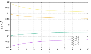
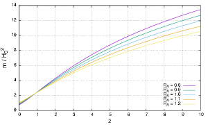
Figure 1: $k(r(z))/H_{0}^{2}$(left) and $m(r(z))/H_{0}^{2}$(right) are depicted as functions of $z$ for several values of $\mathcal{R}_{\Lambda}$.

In these $\Lambda$LTB models, we can evaluate the density distribution on the present time slice $t=t_{0}$, where $t_{0}$ can be evaluated by

$$t_{0}=\int^{1}_{0}\frac{\mathrm{d}X}{\sqrt{f(0,X)}}.$$ (48)

In order to obtain $\rho(t_{0},r)$ from Eq. (4), we need to calculate $S(t_{0},r)$ and $\partial_{r}S(t_{0},r)$ as functions of $r$. $S(t_{0},r)$ can be calculated by numerically solving Eq. (7) with $t=t_{0}$. Then, we can obtain $\partial_{r}S(t_{0},r)$ by numerically solving Eq. (22). We note that the hypersurface $t=t_{0}$ is a spacelike hypersurface and the quantity $\rho(t_{0},r)$ is not a direct observable. Observational aspects are discussed elsewhere, and we simply use $\rho(t_{0},r)$ to demonstrate the inhomogeneity in this paper. Let us define the density fluctuation $\Delta_{0}$ as

$$\Delta_{0}(t_{0},r_{\rm lc}(z)):=\frac{\rho(t_{0},r_{\rm lc}(z))-\rho(t_{0},r_{\rm lc}(10))}{\rho(t_{0},r_{\rm lc}(10))}.$$ (49)

It should be noted that, although we describe $\Delta_{0}$ as a function of $z$, $\Delta_{0}(t_{0},r_{\rm lc}(z))$ is defined on the spacelike surface $t=t_{0}$. The redshift $z$ is simply used to specify the radial coordinate $r$.

In Fig. 2, we show the density fluctuation $\Delta_{0}(t_{0},r_{\rm lc}(z))$ as a function of $z$ and the value of $\Delta_{0}(t_{0},0)$ for several values of $\mathcal{R}_{\Lambda}$.

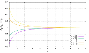
Figure 2: (left)$\Delta_{0}(t_{0},r_{\rm lc}(z))$ is depicted as a function of $z$ for several values of $\mathcal{R}_{\Lambda}$. (right)The value of $\Delta_{0}(t_{0},0)$ is depicted for several values of $\mathcal{R}_{\Lambda}$.

As is shown in Fig. 2, we obtain void(over dense) structures for $\mathcal{R}_{\Lambda}<1(>1)$ around the symmetry center. The magnitude of the density inhomogeneity is roughly proportional to the value of $\mathcal{R}_{\Lambda}$ and $\Delta_{0}(t_{0},0)\sim-0.25$ for $\mathcal{R}_{\Lambda}=0.8$.

VI Summary and discussion

In this paper, we have described technical details of the construction of the $\Lambda$LTB model for a given set of a distance-redshift relation and a value of $\Lambda$ with the bang time function being constant. It has been shown that we can obtain a unique $\Lambda$LTB model for each set of $\Lambda$ and a distance-redshift relation. As a demonstration, we have constructed the $\Lambda$LTB model whose distance-redshift relation is given by that in the flat $\Lambda$CDM model with the cosmological parameters $(\Omega^{\rm dis}_{\rm m0},\Omega^{\rm dis}_{\rm\Lambda 0})=(0.3,0.7)$. As is expected from previous works, we obtain void type structure for a smaller value of $\Lambda$ compared with $3\Omega^{\rm dis}_{\rm\Lambda 0}H_{0}^{2}$.

The method of the inverse construction can be a complement to the conventional method in which LTB functions($k(r)$, $M(r)$ and $t_{\rm B}(r)$ in the text) are directly parametrized by using several parameters(see, e.g. Ref. Redlich:2014gga ). The models given by solving the inverse construction problem may be significantly different from the models given by the direct parametrization of the LTB functions. Therefore, it is important to combine the inverse construction method and analyses with observational data(see, e.g. Ref. Sundell:2015cza ). We will report the CMB and local Hubble parameter analysis combined with our inverse construction method elsewherewithIchiki .

VII Acknowledgements

We thank K. Ichiki, K. Nakao and H. Negishi for helpful comments. C.Y. was partially supported by Grant-in-Aid for Young Scientists (B) Grant Number JP16K17688 and Grant-in-Aid for Scientific Research on Innovative Areas Grant Number JP16H01097.

References

- (1) I. Zehavi, A. G. Riess, R. P. Kirshner, and A. Dekel, Astrophys. J. 503, 483 (1998), arXiv:astro-ph/9802252, A Local Hubble Bubble from SNe Ia?
- (2) M.-N. Celerier, Astron. Astrophys. 353, 63 (2000), arXiv:astro-ph/9907206, Do we really see a cosmological constant in the supernovae data ?
- (3) K. Tomita, Astrophys. J. 529, 38 (2000), arXiv:astro-ph/9906027, Distances and lensing in cosmological void models.
- (4) H. Alnes, M. Amarzguioui, and O. Gron, Phys. Rev. D73, 083519 (2006), arXiv:astro-ph/0512006, An inhomogeneous alternative to dark energy?
- (5) M. Redlich, K. Bolejko, S. Meyer, G. F. Lewis, and M. Bartelmann, Astron. Astrophys. 570, A63 (2014), arXiv:1408.1872, Probing spatial homogeneity with LTB models: a detailed discussion.
- (6) J. Garcia-Bellido and T. Haugboelle, JCAP 0809, 016 (2008), arXiv:0807.1326, Looking the void in the eyes - the kSZ effect in LTB models.
- (7) J.-P. Uzan, C. Clarkson, and G. F. R. Ellis, Phys. Rev. Lett. 100, 191303 (2008), arXiv:0801.0068, Time drift of cosmological redshifts as a test of the Copernican principle.
- (8) C.-M. Yoo, T. Kai, and K.-i. Nakao, Prog. Theor. Phys. 120, 937 (2008), arXiv:0807.0932, Solving Inverse Problem with Inhomogeneous Universe.
- (9) M. Quartin and L. Amendola, Phys. Rev. D81, 043522 (2010), arXiv:0909.4954, Distinguishing Between Void Models and Dark Energy with Cosmic Parallax and Redshift Drift.
- (10) C.-M. Yoo, T. Kai, and K.-i. Nakao, Phys. Rev. D83, 043527 (2011), arXiv:1010.0091, Redshift Drift in LTB Void Universes.
- (11) K. Yagi, A. Nishizawa, and C.-M. Yoo, JCAP 1204, 031 (2012), arXiv:1112.6040, Direct Measurement of the Positive Acceleration of the Universe and Testing Inhomogeneous Models under Gravitational Wave Cosmology.
- (12) N. Mustapha, C. Hellaby, and G. F. R. Ellis, Mon. Not. Roy. Astron. Soc. 292, 817 (1997), arXiv:gr-qc/9808079, Large scale inhomogeneity versus source evolution: Can we distinguish them observationally?
- (13) T. H.-C. Lu and C. Hellaby, Class. Quant. Grav. 24, 4107 (2007), arXiv:0705.1060, Obtaining the spacetime metric from cosmological observations.
- (14) M. L. McClure and C. Hellaby, Phys. Rev. D78, 044005 (2008), arXiv:0709.0875, The Metric of the Cosmos II: Accuracy, Stability, and Consistency.
- (15) M.-N. Celerier, K. Bolejko, and A. Krasinski, Astron. Astrophys. 518, A21 (2010), arXiv:0906.0905, A (giant) void is not mandatory to explain away dark energy with a Lemaitre – Tolman model.
- (16) E. W. Kolb and C. R. Lamb, (2009), arXiv:0911.3852, Light-cone observations and cosmological models: implications for inhomogeneous models mimicking dark energy.
- (17) P. Dunsby, N. Goheer, B. Osano, and J.-P. Uzan, JCAP 1006, 017 (2010), arXiv:1002.2397, How close can an Inhomogeneous Universe mimic the Concordance Model?
- (18) H. Iguchi, T. Nakamura, and K.-i. Nakao, Prog. Theor. Phys. 108, 809 (2002), arXiv:astro-ph/0112419, Is dark energy the only solution to the apparent acceleration of the present universe?
- (19) D. J. H. Chung and A. E. Romano, Phys. Rev. D74, 103507 (2006), arXiv:astro-ph/0608403, Mapping Luminosity-Redshift Relationship to LTB Cosmology.
- (20) R. A. Vanderveld, E. E. Flanagan, and I. Wasserman, Phys. Rev. D74, 023506 (2006), arXiv:astro-ph/0602476, Mimicking Dark Energy with Lemaitre-Tolman-Bondi Models: Weak Central Singularities and Critical Points.
- (21) A. E. Romano, Phys. Rev. D82, 123528 (2010), arXiv:0912.4108, Mimicking the cosmological constant for more than one observable with large scale inhomogeneities.
- (22) A. E. Romano, JCAP 1005, 020 (2010), arXiv:0912.2866, Can the cosmological constant be mimicked by smooth large-scale inhomogeneities for more than one observable?
- (23) A. Krasinski, Phys. Rev. D90, 064021 (2014), arXiv:1407.2862, Mimicking acceleration in the constant-bang-time Lemaître-Tolman model: Shell crossings, density distributions, and light cones.
- (24) A. E. Romano, H.-W. Chiang, and P. Chen, Class. Quant. Grav. 31, 115008 (2014), arXiv:1312.4458, A new method to determine large scale structure from the luminosity distance.
- (25) C.-M. Yoo, Prog. Theor. Phys. 124, 645 (2010), arXiv:1010.0530, A Note on the Inverse Problem with LTB Universes.
- (26) A. E. Romano and P. Chen, JCAP 1110, 016 (2011), arXiv:1104.0730, Corrections to the apparent value of the cosmological constant due to local inhomogeneities.
- (27) H. Negishi, K.-i. Nakao, C.-M. Yoo, and R. Nishikawa, Phys. Rev. D92, 103003 (2015), arXiv:1505.02472, Systematic error due to isotropic inhomogeneities.
- (28) W. Valkenburg, Gen. Rel. Grav. 44, 2449 (2012), arXiv:1104.1082, Complete solutions to the metric of spherically collapsing dust in an expanding spacetime with a cosmological constant.
- (29) A. Krasinski, Phys. Rev. D90, 023524 (2014), arXiv:1405.6066, Accelerating expansion or inhomogeneity? II. Mimicking acceleration with the energy function in the Lemaitre-Tolman model.
- (30) P. Sundell and I. Vilja, (2016), arXiv:1601.05256, Inhomogeneity of the LTB models.
- (31) P. Sundell, E. Mortsell, and I. Vilja, JCAP 1508, 037 (2015), arXiv:1503.08045, Can a void mimic the in CDM?
- (32) M. Tokutake, C.-M. Yoo, and K. Ichiki, in preparation.