Kubo-Greenwood approach to conductivity in dense plasmas with average atom models

Abstract

A new formulation of the Kubo-Greenwood conductivity for average atom models is given. The new formulation improves upon previous by explicitly including the ionic-structure factor. Calculations based on this new expression lead to much improved agreement with ab initio results for DC conductivity of warm dense hydrogen and beryllium, and for thermal conductivity of hydrogen. We also give and test a slightly modified Ziman-Evans formula for the resistivity that includes a non-free electron density of states, thus removing an ambiguity in the original Ziman-Evans formula. Again results based on this expression are in good agreement with ab initio simulations for warm dense beryllium and hydrogen. However, for both these expressions, calculations of the electrical conductivity of warm dense aluminum lead to poor agreement at low temperatures compared to ab initio simulations.

I Introduction

An important aspect of modeling warm and hot dense matter is the calculation of electron thermal and electrical conductivities. The former is of particular relevance in the field of inertial confinement fusion lambert11 ; hu14 where it is the main phenomena that determines the ablation of the cold deuterium/tritium fuel. Currently we have no reliable model that can predict accurate thermal and electrical conductivities across all temperature and density regimes of interest. In particular, as we move out of the degenerate electron regime the gold standard method of Kohn-Sham density functional theory molecular dynamics (KS-DFT-MD) coupled with the Kubo-Greenwood formalism kubo57 ; greenwood58 ; hanson11 ; desjarlais02 quickly becomes computationally prohibitive. In the degenerate, or nearly degenerate regimes, this method is thought to be accurate and agrees with experiments for materials under normal conditions sjostrom15 .

Average atom models provide an computationally efficient alternative at the cost of physical accuracy. The central idea is that one tries to calculate the properties of one atom in the plasma that is supposed to represent the average of all atoms in the plasma. Average atom models have been used successfully for many years for equation of state calculations feynman ; liberman ; piron3 ; wilson ; scaalp ; rozsnyai . They have also been used for electrical conductivity calculations, primarily by coupling to the Ziman-Evans (ZE) formula sterne07 ; perrot87 ; faussurier15 ; pain10 ; dharma06 ; rozsnyai08 ; burrill16 . Recently, a systemic comparison of calculations of electrical conductivity using this method against Kubo-Greenwood KS-DFT-MD calculations burrill16 showed generally very good agreement between the methods provided that a judicious choice was made when coupling the average atom model to the ZE formula. However, the ZE formula, unlike the KG method, is not easily generalized to thermal conductivity or optical conductivity. The latter is useful as it can by used to calculate other optical properties, including the opacity and reflectivity mazevet03 .

A formulation of the Kubo-Greenwood method for average atoms models has been developed by Johnson and co-workers johnson ; johnson09 ; johnson2 . However, a subsequent systematic analysis of the method compared to KS-DFT-MD showed some serious inaccuracies starrett12a . Unlike the ZE formulation, Johnson’s KG formulation does make not explicit account of the ion-ion structure factor $S(k)$. In this work, we give an alternative derivation of the KG formulation for average atom models that explicitly accounts for $S(k)$. The new formulation recovers Johnson’s result when $S(k)=1$. We also give the equations for thermal and optical conductivity.

To evaluate this new formulation we make comparisons to KS-DFT-MD calculations for hydrogen lambert11 and beryllium hanson11 . We also compare to other models faussurier15 ; sjostrom15 and experiments for aluminum milchberg88 ; sperling15 . We use the recently developed pseudo-atom molecular dynamics (PAMD) starrett15 ; starrett13 to generate the necessary inputs for the KG equation.

In addition to this, we present a slightly modified Ziman-Evans formula that takes into account a non-free electron density of states (DOS). The original ZE formula assumes a free electron DOS and this leads to an ambiguity in the choice of chemical potential and density of scattering electrons. This point was discussed in detail in burrill16 . The present reformulation recovers the original form of the ZE equation when the DOS goes to the free electron form and removes the ambiguity when the DOS is not free electron like. We compare calculations based on this new ZE formulation to the new KG formulation and to the KS-DFT-MD results.

The structure of this paper is as follows. In section II we derive the Kubo-Greenwood expression for average atom models with explicit account of the ion-ion structure factor. We also give the expression for the thermal conductivity. In section III we show how the Ziman-Evans formula for the inverse resistivity is modified to account for a non-free electron density of states. In section IV we discuss the connection of these formulas to the the Pseudo-Atom Molecular Dynamics (PAMD) average atom model. In section V we use the PAMD model with the new KG and ZE expressions to calculate the DC electrical conductivity of warm dense hydrogen, beryllium and aluminum, and compare to available simulations, models and experiments. For hydrogen we also compare thermal conductivity calculations to KS-DFT-MD simulation results. Lastly, in section VI we draw our conclusions. Throughout we use Hartree atomic units in which $\hbar=m_{e}=e=1$.

II Kubo-Greenwood approximation

The Kubo-Greenwood expression for the conductivity is greenwood58

$$\sigma(\omega) = \frac{-2\pi}{V}\int\,d\epsilon\,\frac{f(\epsilon_{m})-f(\epsilon_{n})}{\omega}\int\,d^{3}k_{m}\,\int\,d^{3}k_{n}\,$$ (1)

$$\times\left<\left|J_{mn}\right|^{2}\right>\delta(\epsilon_{m}-\epsilon-\omega)\delta(\epsilon_{n}-\epsilon)$$

with

$$J_{mn}\equiv\int_{V}\,d^{3}r\,\psi_{{\bm{k}}_{m}}^{*}(\bm{r})\hat{\bm{v}}_{z}\psi_{{\bm{k}}_{n}}(\bm{r})$$ (2)

where $\epsilon_{n(m)}=k_{n(m)}^{2}/2$ is the energy of the initial (final) electron state and $\psi_{{\bm{k}}_{n(m)}}({\bm{r}})$ is the corresponding wave function, $f(\epsilon)$ is the Fermi-Dirac occupation factor and $\hat{\bm{v}}_{z}$ is the velocity operator in the $\hat{\bm{z}}$ direction. Following Evans evans73 , we now assume that the potential felt by a electron is of muffin-tin form. In this widely used approximation the total scattering potential is the sum of non-overlapping potentials, centered on each nuclear site. Each muffin-tin potential is contained in a sphere of volume $V_{MT}$. Again following Evans evans73 we further assume that the wave function inside each sphere the wave function is given by

$$\psi_{{\bm{k}}_{n}}(\bm{r})=\bar{\psi}_{{\bm{k}}_{n}}(\bm{r})e^{\imath{\bm{k}}_{n}\cdot{\bm{R}}_{\alpha}}$$ (3)

where

$$\bar{\psi}_{{\bm{k}}_{n}}(\bm{r})=\sum_{l}\sum_{m}\imath^{l}e^{\imath\delta_{l}(k_{n})}Y_{lm}(\hat{{\bm{k}}_{n}})Y_{lm}^{*}(\hat{{\bm{r}}_{n}})\frac{y_{l}(r,k_{n})}{r\sqrt{k}}$$ (4)

Here ${\bm{R}}_{\alpha}$ is the position vector of nucleus $\alpha$. Further assuming that each muffin tin potential is identical and using the definition of the ion-ion structure factor:

$$S(k)=\frac{1}{N}\left<\rho_{{\bm{k}}}\rho_{-{{\bm{k}}}}\right>$$ (5)

where

$$\rho_{\bm{k}}=\sum_{\alpha=1}^{N}e^{\imath{\bm{k}}\cdot{\bm{R}}_{\alpha}}$$ (6)

the Kubo-Greenwood conductivity expression is reduced to

$$\sigma(\omega) = -2\pi n_{I}^{0}\int\,d\epsilon\,\frac{f(\epsilon_{m})-f(\epsilon_{m})}{\omega}\int\,d\hat{{\bm{k}}}_{m}\,\int\,d\hat{{\bm{k}}}_{n}\,$$ (7)

$$\times|\sqrt{k_{n}\,k_{m}}\bar{J}_{mn}|^{2}S(|{{\bm{k}}_{n}}-{{\bm{k}}_{m}}|)$$

where $\epsilon_{m}=\epsilon+\omega$, $\epsilon_{n}=\epsilon$, $n_{I}^{0}=N/V$

$$\bar{J}_{mn}\equiv\int_{V_{MT}}\,d^{3}r\,\bar{\psi}_{{\bm{k}}_{m}}^{*}(\bm{r})\hat{\bm{v}}_{z}\bar{\psi}_{{\bm{k}}_{n}}(\bm{r})$$ (8)

Using equation (4) in (7) and after some lengthy algebra (see appendix) we arrive at the result

$$\sigma(\omega)=\sigma^{(1)}(\omega)+\sigma^{(2)}(\omega)+\sigma^{(3)}(\omega)$$ (9)

with

$$\sigma^{(1)}(\omega) = -2\pi n_{I}^{0}\int\,d\epsilon\,\frac{f(\epsilon_{m})-f(\epsilon_{m})}{\omega}$$ (10)

$$\!\!\!\!\!\!\!\!\!\!\!\!\!\!\!\!\!\!\!\!\!\!\!\!\times\sum_{l=0}^{\infty}|I_{A}(l)|^{2}\frac{(l+1)}{2(2l+3)}\left[(1+\frac{l}{2})I_{s}^{(1)}+\frac{l}{2}I_{s}^{(2)}\right]$$

$$\sigma^{(2)}(\omega) = 2\pi n_{I}^{0}\int\,d\epsilon\,\frac{f(\epsilon_{m})-f(\epsilon_{m})}{\omega}$$ (11)

$$\!\!\!\!\!\!\!\!\!\!\!\!\!\!\!\!\!\!\!\!\!\!\!\!\times\sum_{l=0}^{\infty}I_{A}(l)I_{B}(l+2)\cos(\delta_{l}(k_{n})-\delta_{l+2}(k_{n}))$$

$$\!\!\!\!\!\!\!\!\!\!\!\!\!\!\!\!\!\!\!\!\!\!\!\!\times\frac{(l+1)(l+2)}{2(2l+3)}\left[3\,I_{s}^{(2)}-I_{s}^{(1)}\right]$$

$$\sigma^{(3)}(\omega) = -2\pi n_{I}^{0}\int\,d\epsilon\,\frac{f(\epsilon_{m})-f(\epsilon_{m})}{\omega}$$ (12)

$$\!\!\!\!\!\!\!\!\!\!\!\!\!\!\!\!\!\!\!\!\!\!\!\!\!\!\!\!\!\!\!\!\!\!\!\!\times\sum_{l=0}^{\infty}|I_{B}(l)|^{2}\frac{l}{4(2l-1)}\left[(l-1)I_{s}^{(1)}+(l+1)I_{s}^{(2)}\right]$$

where

$$I_{s}^{(1)}\equiv\int_{-1}^{1}dx\,S(\sqrt{(k_{n}^{2}+k_{m}^{2}-2k_{n}k_{m}\,x)})$$ (13)

$$I_{s}^{(2)}\equiv\int_{-1}^{1}dx\,x^{2}\,S(\sqrt{(k_{n}^{2}+k_{m}^{2}-2k_{n}k_{m}\,x)})$$ (14)

and $I_{A}$ and $I_{B}$ are the same as in reference starrett12a ,

$$I_{A}(l,k_{n},k_{m}) \equiv \int\limits_{0}^{R_{MT}}dr\,y_{l+1}(r,k_{m})$$ (15)

$$\!\!\!\!\!\!\!\!\!\!\!\times\left(\frac{\partial y_{l_{i}}(r,k_{n})}{\partial r}-(l+1)\frac{y_{l}(r,k_{n})}{r}\right)$$

$$I_{B}(l,k_{n},k_{m}) \equiv \int\limits_{0}^{R_{MT}}dr\,y_{l-1}(r,k_{m})$$ (16)

$$\!\!\!\!\!\!\!\!\!\!\!\times\left(\frac{\partial y_{l_{i}}(r,k_{n})}{\partial r}+l\frac{y_{l}(r,k_{n})}{r}\right)$$

In the limit $S(k)\to 1$ $\forall k$, $\sigma^{(2)}(\omega)=0$ and the expression for the conductivity is reduced to that of Johnson’s result johnson ; starrett12a provided that the integral over the muffin tin volume $V^{MT}=4/3\pi R_{MT}^{3}$ is instead taken over all space. We return to this point in section IV

As shown in reference starrett12a the thermal conductivity $\kappa$ can be calculated in a straight forward extension. For a plasma of temperature $T$

$$\kappa=\frac{1}{T}\left({\cal L}_{22}-\frac{{\cal L}_{12}^{2}}{{\cal L}_{11}}\right)$$ (17)

where

$${\cal L}_{nm}= = (-1)^{n+m}2\pi n_{I}^{0}\int\,d\epsilon\,(\epsilon-\mu_{e})^{n+m-2}$$ (18)

$$\times\frac{\partial f(\epsilon)}{\partial\epsilon}\int\,d\hat{{\bm{k}}}_{m}\,\int\,d\hat{{\bm{k}}}_{n}\,$$

$$\times|\sqrt{k_{n}\,k_{m}}\bar{J}_{mn}|^{2}S(|{{\bm{k}}_{n}}-{{\bm{k}}_{m}}|)$$

Clearly, $\sigma_{DC}=\sigma(0)={\cal L}_{11}$. The Lorenz number is defined as

$$L=\frac{\kappa}{T\sigma_{DC}}$$ (19)

For fully degenerate electrons this takes the value $L=\pi^{2}/3$, while for fully non-degenerate electrons this takes the value 1.597. Lastly we note that the extension of this formulation to mixtures is straightforward, but is not explored here.

III Ziman-Evans expression with an explicit density of states

The Ziman-Evans expression for the inverse conductivity $R$ is ziman61 ; evans73

$$R=\frac{1}{\sigma_{DC}}=-\frac{1}{3\pi^{2}(n_{e}^{*})^{2}}\int_{0}^{\infty}d\epsilon\frac{df}{d\epsilon}v^{3}\frac{1}{\tau_{p}}$$ (20)

where $n_{e}^{*}$ is the density of scattering electrons and $f(\epsilon,\mu_{e}^{*})$ is the Fermi-Dirac occupation factor and we have expanded the notation to indicate that it depends on the chemical potential $\mu_{e}^{*}$. The relaxation time $\tau_{p}$ is defined in terms of the generalized momentum transport cross section

$$\sigma_{TR}(p)=2\pi\int_{0}^{\pi}d\theta|T_{{\bm{p}}{{\bm{p}}}^{\prime}}|^{2}(1-\cos\theta)\sin\theta$$ (21)

and the transition matrix element $T_{{\bm{p}}{{\bm{p}}}^{\prime}}$ is given by evans73

$$|T_{{\bm{p}}{{\bm{p}}}^{\prime}}|^{2}=\frac{d\sigma}{d\theta}(p,\theta)S(q)$$ (22)

where $q^{2}=2p^{2}(1-\cos\theta)$, and $S(q)$ is the ion-ion structure factor and $d\sigma/d\theta$ is the differential scattering cross section burrill16 . ${\bm{p}}$ (${{\bm{p}}}^{\prime}$) is the initial (final) momentum of the electron before (after) the collision with the atom. Only elastic collisions are included, in which $|{\bm{p}}|=|{{\bm{p}}}^{\prime}|$. The final result for the relaxation time is

$$\frac{1}{\tau_{p}}=\pi n_{I}^{0}\frac{v}{p^{4}}\,\int_{0}^{2p}dq\,q^{3}\frac{d\sigma}{d\theta}(p,\theta)S(q)$$ (23)

where $p=m_{e}v=\sqrt{2\epsilon}$.

As explained in reference burrill16 a challenge when using equation (20) is the ambiguity in what one should choose for $n_{e}^{*}$ and $\mu_{e}^{*}$. This is due to the implicit free-electron density of states. Equation (20) is modified to include a non-free electron density of states by introducing a factor $N_{e}(\epsilon)$ into the integrand potekhin96 :

$$R=\frac{1}{(n_{e}^{*})^{2}}\int_{0}^{\infty}d\epsilon\left(-\frac{df}{d\epsilon}\right)N_{e}(\epsilon)\frac{1}{\tau_{p}}$$ (24)

where

$$N_{e}(\epsilon)=n_{I}^{0}\int_{0}^{\epsilon}d\epsilon^{\prime}\chi(\epsilon^{\prime})$$ (25)

$\chi(\epsilon)$ is the density of states such that the number of valence electrons per atom $\bar{Z}$ is

$$\bar{Z}=\frac{\bar{n}_{e}^{0}}{n_{I}^{0}}=\int_{0}^{\infty}d\epsilon\chi(\epsilon)f(\epsilon,\mu_{e})$$ (26)

Here $\mu_{e}$ is the calculated, “physical” chemical potential and $\bar{n}_{e}^{0}$ is the density of valence electrons. Thus we can identify $n_{e}^{*}=\bar{n}_{e}^{0}$ and $\mu_{e}^{*}=\mu_{e}$. Such a choice cannot be used with equation (20) without introducing an inconsistency, and one is forced to compromise (see burrill16 ). In the limit as $T\to 0$ in equation (24) we recover the expected Drude form

$$\frac{1}{R}=\bar{n}_{e}^{0}\,\tau_{v_{F}}$$ (27)

The usual expression for the resistivity (20) is recovered from equation (24) if we take the density of states to be its free electron form

$$\chi^{free}(\epsilon)=\frac{\sqrt{2\epsilon}}{n_{I}^{0}\pi^{2}}$$ (28)

then

$$N_{e}^{free}(\epsilon)=\frac{v^{3}}{3\pi^{2}}$$ (29)

IV Connection to the PAMD model

The above formulations can be used with any model that give access to the electron scattering potential $V^{scatt}$ and the ion-ion structure factor $S(k)$. From the scattering potential one can determine the chemical potential $\mu_{e}$, the wavefunctions $y_{l}(r,k)$, and the density of states $\chi(\epsilon)$. As in reference burrill16 we shall use the pseudo-atom molecular dynamics (PAMD) starrett15 model to generate these inputs. This model had been described in detail elsewhere starrett15 ; starrett13 ; starrett14 and has successfully been used to calculate equation of state, ionic structure and ionic transport daligault16 in the warm and hot dense matter regime. Its connection with the ZE equations was explored in detail in burrill16 . In short, in PAMD the electronic structure of one pseudo-atom in a plasma is calculated using density functional theory (here we restrict ourselves to Kohn-Sham DFT). By coupling this electronic structure to the integral equations of fluid theory (the quantum Ornstein-Zernike (QOZ) equations) one calculates a parameter-free ion-ion pair interaction potential. This can be used in molecular dynamics simulations or, as we have here and in reference burrill16 , directly in the QOZ equations to generate $S(k)$.

As discussed in reference burrill16 there are at least two reasonable choices for the scattering potential: the pseudo-atom potential $V^{PA}(r)$ and the average atom potential $V^{AA}(r)$. The former can be used to construct the total scattering potential of the plasma when combined with a set on nuclear position vectors $\{{\bm{R}}_{i}\}$

$$V^{tot}({\bm{r}})=\sum_{i}V^{PA}(|{\bm{r}}-{\bm{R}}_{i}|)$$ (30)

while the latter $V^{AA}$ is a muffin-tin like potential that extends to the ion-sphere radius. Given the above derivation of the KG formula one would expect $V^{AA}$ to be the most reasonable choice. However, it was found in burrill16 that when using the (similarly derived) ZE formulation $V^{PA}$ gives generally much better agreement with KS-DFT-MD results that are thought to be accurate. This surprising result was explained by realizing that in the Born limit of scattering (i.e. where the scattered state is a plane wave) the total scattering cross section separates into a sum over cross sections for each atom. In that limit the total scattering cross section is given by the Fourier transform of $V^{tot}$. Thus to recover the Born limit it is necessary to use the $V^{PA}$ potential. Though this choice violates the condition of non-overlapping muffin-tins, it compensates for the neglect of multiple scattering effects in our wavefunctions by essentially treating them in the Born approximation, while allowing strong single site scattering though the use of the t-matrix approximation.

In the KG formulation we similarly neglect multiple scattering contributions and we might expect the same potential ($V^{PA}$) to also lead to improved results, again letting the muffin tin volume being replaced by a integral over all space. We note that in Johnson’s formulation johnson , where $S(k)=1$, the $V^{AA}$ potential is used and the integral is taken over all space. There, the physical model is an average atom model in jellium. One could restrict the integrals to be inside the muffin-tin (ion-sphere) volume only, but this results in conductivities that are orders of magnitude incorrect! The reason for this gross error was first suggested in reference dulca00 . In that work the isolated cluster method (ICM) was use to calculate conductivity of clusters of atoms with up to 201 atoms using the real-space Green’s function method. The average atom model is essentially an ICM with one atom starrett15a . In reference dulca00 they found that the conductivity was dependent on the size of the cluster and that convergence was not achieved with up to 201 atoms. The explanation given was that the cluster approach can only yield correct results if the mean free path of the electron is approximately equal to, or smaller than, the size of the cluster – if the mean free path of the electron is larger than the the cluster, the scattering processes that lead to a finite conductivity cannot be expected to be accurately modeled in the cluster representation dulca00 . Clearly, here with our neglect of multiple scattering effects, our cluster size is effectively the volume of the ion-sphere, hence unless the resistivity is very large (corresponding to very small mean free paths) the results will be substantially incorrect. By letting the integration volume go to infinity this obviously corrects for this defect. However the price is that, since no other scattering events are included in the electronic wavefunction, the calculated conductivity diverges as $\omega^{-2}$ johnson ! Johnson introduced a practical method to correct for this divergence: the optical conductivity is required to have a Drude like behavior by multiplying by $\omega^{2}/(\gamma^{2}+\omega^{2})$. $\gamma$ is found by enforcing the frequency sum rule

$$\int\limits_{0}^{\infty}d\omega\sigma(\omega)=\frac{n_{I}^{0}\pi\bar{Z}}{2}$$ (31)

where $\bar{Z}$ is the number of valence electrons per ion. We note that we are only considering the free-free contribution to the conductivity here. This combination of letting the integration volume go to infinity and enforcing the Drude form represents a reasonable way of capturing the main effects important to the calculation of the conductivity, but clearly introduces a significant source of uncertainty into the quality of the calculation.

In the next section we present calculations using the KG equation (9) using this infinite volume correction. We show results using the two potentials $V^{PA}$ and $V^{AA}$. For $V^{AA}$ we also show the result with $S(k)=1$, which is the same as Johnson’s formulation johnson , these can be compared to the nearly identical calculations presented in reference starrett12a . We show results from the Ziman-Evans equation with the non-free density of states included, equation (24), that we label ZE-DOS. Our notation is summarized in table 1.

Notation	Description
KG: $V^{PA}$	Equation (9) with wave functions calculated in the $V^{PA}(r)$ potential.
KG: $V^{AA}$	Equation (9) with wave functions calculated in the $V^{AA}(r)$ potential.
KG: $V^{AA}$, $S(k)=1$	Same as KG: $V^{AA}$, but with $S(k)=1$. This is equivalent to Johnson’s formulation johnson .
ZE-DOS: $V^{AA}$ or $V^{PA}$	Equation (24) with either potential.
ZE-$\mu_{e}$	Equation (20) with the “physical” chemical potential (see burrill16 ).
ZE-$\bar{\mu}_{e}$	Equation (20) with the free electron chemical potential (see burrill16 ).

Table 1: Descriptions of notation used in the figures.

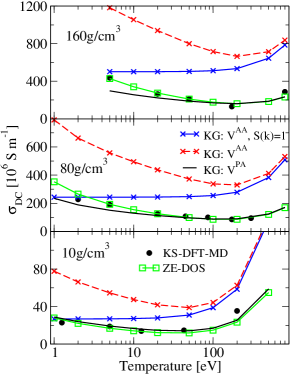
Figure 1: (Color online) Electrical conductivity of dense hydrogen. The KS-DFT-MD results are from reference lambert11 .

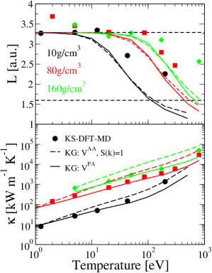
Figure 2: (Color online) Lorenz number and thermal conductivity of dense hydrogen. The KS-DFT-MD results are from reference lambert11 . The horizontal dashed lines for the Lorenz number indicate the degenerate and non-degenerate limits.

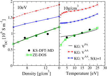
Figure 3: (Color online) Electrical conductivity of dense beryllium. The KS-DFT-MD results are from references starrett12a ; hanson11 .

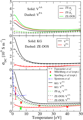
Figure 4: (Color online) Electrical conductivity of solid density (2.7 g/cm³) aluminum.

V Results

In figure 1 we show results for the DC conductivity $\sigma_{DC}$ for dense hydrogen. We compare to KS-DFT-MD results from lambert11 . Clearly both the Ziman-Evans (ZE-DOS) calculations based on equation (24) and the Kubo-Greenwood (KG) calculations based on equation (9) agree well with the KS-DFT-MD results when the pseudoatom potential ($V^{PA}$) is used. A comparison of the ZE-DOS results to those presented in reference burrill16 with the two choices of chemical potential (not shown, but compare to results in reference burrill16 ) reveals little effect from the new formulation, as we would expect, since the two results in burrill16 are similar. Where a difference is seen the ZE-DOS calculations most closely follows the calculations based on the choice $\bar{\mu}_{e}$. KG calculations using $V^{AA}$ are also shown in figure 1. When the structure factor is included the qualitative agreement is reasonable but the quantitative agreement is poor. Without the structure factor, even the qualitative agreement is poor and the results agree with those presented in starrett12a . Therefore the combination of the use of $V^{PA}$ with the inclusion of the ionic structure factor are both vital to find agreement with the KS-DFT-MD results in this case.

In figure 2 we show calculations of the thermal conductivity $\kappa$ and Lorenz number $L$ for the same dense hydrogen conditions as in figure 1. We show calculations using the average atom potential $V^{AA}$ with $S(k)=1$, and using $V^{PA}$. The results using $V^{AA}$ amount to essentially the same calculations as in starrett12a , and the results are very similar, i.e. generally the thermal conductivity overestimates the KS-DFT-MD and the trends are only broadly in agreement. In contrast, the results using $V^{PA}$ agree well with KS-DFT-MD, though some differences at high temperature are found. For the Lorenz number using either potential leads to similar results, and both agree with the degenerate limit at low temperature, and tend to underestimate KS-DFT-MD at high temperature.

In figure 3 we show results for warm dense beryllium. As for hydrogen, using the $V^{AA}$ leads to an overestimation of the KS-DFT-MD results, and using $V^{PA}$ with $S(k)$ from PAMD leads to very good agreement, using either the ZE-DOS or the KG methods. These results, figures 1 to 3, demonstrate that both models introduced in this work can successfully predict conductivities in warm dense matter. For clarity of the figures, we have not shown an explicit comparison for ZE-DOS to the results presented in burrill16 which used the original ZE equation (20) with the two choices of chemical potential (ZE-$\mu_{e}$ and ZE-$\bar{\mu}_{e}$). However, a comparison of the results reveals that ZE-DOS generally lies between the two and closer to ZE-$\bar{\mu}_{e}$ than ZE-$\mu_{e}$.

In figure 4 we show results for warm dense aluminum. Here the situation is much more complicated. In the top panel we show calculations based on the Ziman-Evans formula only. We compare both potentials ($V^{AA}$ and $V^{PA}$) as well as the new ZE-DOS formulation to original ZE formulation with the two choices of chemical potential considered in burrill16 . We find that the results from ZE-DOS agree reasonably closely with ZE-$\bar{\mu}_{e}$ and the the results using $V^{AA}$ are larger than using $V^{PA}$. In the center panel we compare the ZE-DOS results to those using the KG formulation. For the same potential the ZE and KG are reasonably close, but at lowest temperatures KG with $V^{AA}$ gives a somewhat larger conductivity than ZE with the same potential.

In the bottom panel of figure 4 we compare to other calculations and experiments. First there is an experiment due to Milchberg et al milchberg88 and a very recent experiment due to Sperling et al sperling15 . The experiments are in significant disagreement with each other. A recent simulation that post-processes an Orbital Free MD simulation with the Kohn-Sham KG method is also shown (Sjostrom et al sjostrom15 ). In the analysis of reference sjostrom15 they demonstrate that their simulations agree with previous KS-DFT-MD results at lower temperatures as well as other experiments, casting doubt on the veracity of the new measurements of Sperling et al. Finally we also show a calculation of Faussurier et al that uses the SCAALP model faussurier15 . This is a model that is similar in spirit to the PAMD model used here, though differs in details. Their conductivity calculation uses the Ziman-Evans method and is qualitatively most similar to our calculations when we use ZE-$\mu_{e}$ with $V^{AA}$. Comparing the result of Faussurier et al to this calculation (bottom panel) we find good agreement which provides gross check that our calculations are reasonable.

Now comparing our calculations using $V^{PA}$ with ZE-DOS or KG to the simulations of Sjostrom et al we find that while they agree well with each other, they do not agree well the Sjostrom et al sjostrom15 , with our calculations predicting a significantly smaller conductivity. Moreover our results are in agreement with the recent experiment of Sperling et al but underestimate the older experiment of Milchberg et al. Our results using $V^{AA}$ with either ZE-DOS or KG also do not agree well with Sjostrom et al either, though the magnitude is improved. In fact the best agreement with the Sjostrom simulation is found when we emulate the calculation of Faussurier et al (i.e. ZE-$\mu_{e}$: $V^{AA}$). The evidence put forward in Sjostrom et al sjostrom15 suggests that the experiment of Sperling, and in turn our results using $V^{PA}$, are too small. This significant disagreement between these simulations and our $V^{PA}$ results stands in stark contrast to the excellent agreement found for hydrogen and beryllium (figures 1 and 3).

To explain why we find such a strong disagreement in this case we recall the reasoning behind the choice of the electron scattering potential $V^{PA}$. In the limit where the Born approximation is valid (i.e. when the scattered electron can be modeled as a plane wave) the total scattering cross section for the plasma separates into individual scattering cross sections for each ion in the plasma, which depend only on the scattering potential at that site. In the language of the PAMD model this scattering potential is $V^{PA}(r)$. Thus, the obvious approximation when ignoring multiple scattering effects, but wishing to allow strong scattering (i.e. beyond the Born approximation) is to continue to assume that each site scatters the electrons independently, but treat the scattering cross section using the t-matrix approach. In the KG formula the t-matrix is equivalent to using the calculated scattered wavefunctions. Thus we can expect $V^{PA}$ to be a reasonable scattering potential where ever multiple scattering effects can be ignored. One test that would indicate the validity of this assumption is if the Born calculation itself gives reasonable results. In fact, as shown in burrill16 ; cpw15 , Born approximation based calculations using the ZE formula give reasonable results for the hydrogen and Beryllium cases we have looked at here, whereas for aluminum the Born result is in gross error. This is thus the likely reason for the failure of the $V^{PA}$ based calculation for aluminum at the lower temperatures. We stress that it is not a necessary condition that the Born approximation be valid for the present models to be accurate, rather that the multiple scattering effect be negligible. Indeed the t-matrix based calculations presented in burrill16 are in significantly better agreement with the KS-DFT-MD result for hydrogen than corresponding Born approximation results.

As shown in figure 4 , using $V^{AA}$ we get somewhat improved agreement with the simulations of Sjostrom et al. Unlike $V^{PA}$, $V^{AA}$ does not recover the Born limit (leading to the poor results using this potential in figures 1 and 3). Using $V^{AA}$ may partially compensate for the breakdown of the weak multiple scattering effect assumptions, but not in a controlled way. Therefore it is difficult to know for which cases (i.e. element, densities and temperatures) that using $V^{AA}$ will lead to improved agreement. In light of this we must be cautious in interpreting this somewhat improved agreement as evidence that $V^{AA}$ leads to improved agreement in general at low temperature.

VI Conclusions

A new derivation of the Kubo-Greenwood conductivity for average atom models is given. The derivation improves upon the previous derivation of Johnson et al johnson by taking the ionic structure factor explicitly into account. Calculations based on the new expression, using the pseudoatom molecular dynamics model starrett15 to provide the inputs, result in a significant improvement in agreement with KS-DFT-MD simulations for the hydrogen and beryllium plasmas tested. We have also given and tested a version of the Ziman-Evans formula for the resistivity that takes into account a non-free electron density of states. This new expression removes the ambiguity as to the choice of chemical potential and density of scattering electrons that was discussed in details in burrill16 . The new Ziman-Evans formula also gives good agreement with the KS-DFT-MD results for hydrogen and beryllium. We have also given the expression for the thermal conductivity based on the Kubo-Greenwood formulation, and found much improved agreement with KS-DFT-MD results for dense hydrogen.

Calculations from the new Ziman-Evans and Kubo-Greenwood formulas for warm dense aluminum found relatively poor agreement with ab initio simulations. Possible reasons for this are discussed.

Appendix A Aspects of the derivation of the KG formula

When deriving equation (9) we are faced with an integral of the form

$$I \equiv \int d\hat{{\bm{k}}}\int d\hat{{\bm{k}}^{\prime}}S(|{\bm{k}}-{\bm{k}}^{\prime}|)$$ (32)

$$\times Y_{l_{1},m_{1}}(\hat{{\bm{k}}})Y_{l_{2},m_{2}}^{*}(\hat{{\bm{k}}^{\prime}})Y_{l_{3},m_{3}}^{*}(\hat{{\bm{k}}})Y_{l_{4},m_{4}}(\hat{{\bm{k}}^{\prime}})$$

which simplifies to

$$I = \int d\hat{{\bm{k}}}S(k)Y_{l_{1},m_{1}}(\hat{{\bm{k}}})Y_{l_{3},m_{1}}^{*}(\hat{{\bm{k}}})$$ (33)

$$\times\delta_{l_{2},l_{4}}\delta_{m_{2},m_{4}}\delta_{m_{1},m_{3}}$$

where $\delta$ is the Kronecker delta, and $k=\sqrt{k^{2}+{k^{\prime}}^{2}-k\,k^{\prime}\cos\theta_{k}}$. When $S(k)=1$, the integrals in $I$ separate and the result simplifies to $\delta_{l_{2},l_{4}}\delta_{m_{2},m_{4}}\delta_{l_{1},l_{3}}\delta_{m_{1},m_{3}}$. To eliminate the remaining sum of magnetic quantum number $m$ a useful relation is

$$\sum_{m=-l}^{l}m^{2}|Y_{lm}(\hat{{\bm{k}}})|^{2}=\frac{l(l+1)(2l+1)}{8\pi}\sin^{2}\theta_{k}$$ (34)

References

- [1] Flavien Lambert, Vanina Recoules, Alain Decoster, Jean Clerouin, and Michael Desjarlais. On the transport coefficients of hydrogen in the inertial confinement fusion regime a). Physics of Plasmas (1994-present), 18(5):056306, 2011.
- [2] S. X. Hu, L. A. Collins, T. R. Boehly, J. D. Kress, V. N. Goncharov, and S. Skupsky. First-principles thermal conductivity of warm-dense deuterium plasmas for inertial confinement fusion applications. Phys. Rev. E, 89:043105, Apr 2014.
- [3] Ryogo Kubo. Statistical-mechanical theory of irreversible processes. i. general theory and simple applications to magnetic and conduction problems. Journal of the Physical Society of Japan, 12(6):570–586, 1957.
- [4] D.A. Greenwood. The boltzmann equation in the theory of electrical conduction in metals. Proceedings of the Physical Society, 71(4):585, 1958.
- [5] David E. Hanson, Lee A. Collins, Joel D. Kress, and Michael P. Desjarlais. Calculations of the thermal conductivity of national ignition facility target materials at temperatures near 10 ev and densities near 10 g/cc using finite-temperature quantum molecular dynamics. Physics of Plasmas, 18(8), 2011.
- [6] M. P. Desjarlais, J. D. Kress, and L. A. Collins. Electrical conductivity for warm, dense aluminum plasmas and liquids. Phys. Rev. E, 66:025401, Aug 2002.
- [7] Travis Sjostrom and Jérôme Daligault. Ionic and electronic transport properties in dense plasmas by orbital-free density functional theory. Phys. Rev. E, 92:063304, 2015.
- [8] R. P. Feynman, N. Metropolis, and E. Teller. Equations of state of elements based on the generalized fermi-thomas theory. Phys. Rev., 75:1561–1573, May 1949.
- [9] David A. Liberman. Self-consistent field model for condensed matter. Phys. Rev. B, 20:4981–4989, Dec 1979.
- [10] R. Piron and T. Blenski. Variational-average-atom-in-quantum-plasmas (vaaqp) code and virial theorem: Equation-of-state and shock-hugoniot calculations for warm dense al, fe, cu, and pb. Phys. Rev. E, 83:026403, Feb 2011.
- [11] B. Wilson, V. Sonnad, P. Sterne, and W. Isaacs. Purgatorio—a new implementation of the inferno algorithm. Journal of Quantitative Spectroscopy and Radiative Transfer, 99(1–3):658 – 679, 2006. Radiative Properties of Hot Dense Matter.
- [12] Gérald Faussurier, Christophe Blancard, Philippe Cossé, and Patrick Renaudin. Equation of state, transport coefficients, and stopping power of dense plasmas from the average-atom model self-consistent approach for astrophysical and laboratory plasmas. Physics of Plasmas, 17(5), 2010.
- [13] Balazs F. Rozsnyai. Relativistic hartree-fock-slater calculations for arbitrary temperature and matter density. Phys. Rev. A, 5:1137–1149, Mar 1972.
- [14] D.J. Burrill, D.V. Feinblum, M.R.J. Charest, and C.E. Starrett. Comparison of electron transport calculations in warm dense matter using the ziman formula. High Energy Density Physics, 19:1 – 10, 2016.
- [15] Gérald Faussurier and Christophe Blancard. Resistivity saturation in warm dense matter. Phys. Rev. E, 91:013105, Jan 2015.
- [16] P.A. Sterne, S.B. Hansen, B.G. Wilson, and W.A. Isaacs. Equation of state, occupation probabilities and conductivities in the average atom purgatorio code. High Energy Density Physics, 3(1–2):278 – 282, 2007. Radiative Properties of Hot Dense Matter.
- [17] François Perrot and M. W. C. Dharma-wardana. Electrical resistivity of hot dense plasmas. Phys. Rev. A, 36:238–246, Jul 1987.
- [18] J.C. Pain and G. Dejonghe. Electrical resistivity in warm dense plasmas beyond the average-atom model. Contributions to Plasma Physics, 50(1):39–45, 2010.
- [19] M. W. C. Dharma-wardana. Static and dynamic conductivity of warm dense matter within a density-functional approach: Application to aluminum and gold. Phys. Rev. E, 73:036401, Mar 2006.
- [20] Balazs F. Rozsnyai. Electron scattering in hot/warm plasmas. High Energy Density Physics, 4(1):64–72, 2008.
- [21] S. Mazevet, L.A. Collins, N.H. Magee, J.D. Kress, and J.J. Keady. Quantum molecular dynamics calculations of radiative opacities. Astronomy & Astrophysics, 405(1):L5–L9, 2003.
- [22] W.R. Johnson, C. Guet, and G.F. Bertsch. Optical properties of plasmas based on an average-atom model. Journal of Quantitative Spectroscopy and Radiative Transfer, 99(1–3):327 – 340, 2006. Radiative Properties of Hot Dense Matter.
- [23] W.R. Johnson. Low-frequency conductivity in the average-atom approximation. High Energy Density Physics, 5(1–2):61 – 67, 2009.
- [24] M. Yu. Kuchiev and W. R. Johnson. Low-frequency plasma conductivity in the average-atom approximation. Phys. Rev. E, 78:026401, Aug 2008.
- [25] C. E. Starrett, J Clérouin, V Recoules, J. D. Kress, L. A. Collins, and D. E. Hanson. Average atom transport properties for pure and mixed species in the hot and warm dense matter regimes. Physics of Plasmas (1994-present), 19(10):102709, 2012.
- [26] H. M. Milchberg, R. R. Freeman, S. C. Davey, and R. M. More. Resistivity of a simple metal from room temperature to k. Phys. Rev. Lett., 61:2364–2367, Nov 1988.
- [27] P. Sperling, E. J. Gamboa, H. J. Lee, H. K. Chung, E. Galtier, Y. Omarbakiyeva, H. Reinholz, G. Röpke, U. Zastrau, J. Hastings, L. B. Fletcher, and S. H. Glenzer. Free-electron x-ray laser measurements of collisional-damped plasmons in isochorically heated warm dense matter. Phys. Rev. Lett., 115:115001, 2015.
- [28] C. E. Starrett, J. Daligault, and D. Saumon. Pseudoatom molecular dynamics. Phys. Rev. E, 91:013104, Jan 2015.
- [29] C. E. Starrett and D. Saumon. Electronic and ionic structures of warm and hot dense matter. Phys. Rev. E, 87:013104, Jan 2013.
- [30] R. Evans, B. L. Gyorfey, N. Szabo, and J. M. Ziman. On the resistivity of liquid transition metals. In S. Takeuchi, editor, The properties of liquid metals. Taylor and Francis, London, 1973.
- [31] J.M. Ziman. A theory of the electrical properties of liquid metals. i: The monovalent metals. Philosophical Magazine, 6(68):1013–1034, 1961.
- [32] A. Yu Potekhin and D.G. Yakovlev. Electron conduction along quantizing magnetic fields in neutron star crusts. ii. practical formulae. Astronomy and Astrophysics, 314:341–352, 1996.
- [33] C.E. Starrett and D. Saumon. A simple method for determining the ionic structure of warm dense matter. High Energy Density Physics, 10:35 – 42, 2014.
- [34] Jérôme Daligault, Scott D. Baalrud, Charles E. Starrett, Didier Saumon, and Travis Sjostrom. Ionic transport coefficients of dense plasmas without molecular dynamics. Phys. Rev. Lett., 116:075002, 2016.
- [35] Paul AM Dirac. Note on exchange phenomena in the thomas atom. Proceedings of the Cambridge Philosophical Society, 26:376, 1930.
- [36] Valentin V. Karasiev, Travis Sjostrom, James Dufty, and S. B. Trickey. Accurate homogeneous electron gas exchange-correlation free energy for local spin-density calculations. Phys. Rev. Lett., 112:076403, Feb 2014.
- [37] Lucian Dulca, John Banhart, and Gerd Czycholl. Electrical conductivity of finite metallic systems: Disorder. Phys. Rev. B, 61:16502–16513, 2000.
- [38] C.E. Starrett. A green’s function quantum average atom model. High Energy Density Physics, 16:18 – 22, 2015.
- [39] D. Burrill, D. Feinblum, M. Charest, and C. Starrett. Modeling warm dense matter using quantum-mechanical density function theory. Los Alamos National Laboratory Computational Physics Workshop 2015 report, 2015.