High-Throughput Prediction of Finite-Temperature Properties using the Quasi-Harmonic Approximation

Abstract

In order to calculate thermal properties in automatic fashion, the Quasi-Harmonic Approximation (QHA) has been combined with the Automatic Phonon Library (APL) and implemented within the AFLOW framework for high-throughput computational materials science. As a benchmark test to address the accuracy of the method and implementation, the specific heats capacities, thermal expansion coefficients, Grüneisen parameters and bulk moduli have been calculated for 130 compounds. It is found that QHA-APL can reliably predict such values for several different classes of solids with root mean square relative deviation smaller than 28% with respect to experimental values. The automation, robustness, accuracy and precision of QHA-APL enable the computation of large material data sets, the implementation of repositories containing thermal properties, and finally can serve the community for data mining and machine learning studies.

1 Introduction

The characterization and prediction of thermal properties of materials are amongst the key factors enabling a rational accelerated materials development [1]. Important properties include specific heat capacity at constant volume/pressure ($C_{V}$ or $C_{p}$), mode resolved and average Grüneisen parameters ($\gamma_{qj}$ and $\gamma$), thermal expansion coefficient ($\alpha_{V}$), Debye temperature ($\theta_{D}$), lattice thermal conductivity ($\kappa_{L}$), and vibrational entropy and Gibbs free energy ($S(p,T)$ and $G(p,T,V)$).

There are several computational techniques leading to the characterization of these thermal properties: i. First principles molecular dynamics (extremely time consuming and computationally impractical for creating large datasets); ii. The GIBBS approach [2] also implemented in the AFLOW-AGL (Automatic-Gibbs-Library) [3] (very fast and reasonably reliable especially for high-throughput screening [1]); iii. Anharmonic force constant calculations and Boltzmann Transport Equation solvers, as implemented in ShengBTE[4], PHONO3PY [5] and in the AFLOW-APL2 Library [6] (computationally intensive but capable of giving very accurate values for $\kappa_{L}$); iv. approaches based on the QHA [7, 8, 9, 10, 11, 12, 13, 14] which can rapidly characterize $C_{V}$, $C_{p}$, $\gamma$, and $\alpha_{V}$. Methods ii-iv. are based on phonon calculations as available in packages like AFLOW-APL [15, 16], PHONOPY [17], Phon [10], ALAMODE [18].

With the goal of creating large repositories of ab-initio calculated properties, such as in our AFLOW.org [19, 20, 21] online database, we have undertaken the task of implementing the quasi-harmonic method in the AFLOW software platform [15]. The quasi-harmonic method is based on the construction of a strain dependent free energy function in which each strained structure belongs to the harmonic regime. The strain dependent free energy contributes as a vibrational energy and introduces anharmonic effects into the system, including the temperature dependence. Although this method has been successfully applied for decades, it has limitations: the QHA loses predictive power when anharmonic forces play a major role in the dynamics (as in the case of thermal conductivity), under extreme conditions in term of temperature and pressure, [22, 23] or close to their melting point [24]. Despite these limitations, this model has been satisfactorily demonstrated to accurately and robustly predict many temperature-dependent properties for compounds of different nature [25, 26, 27, 28, 29, 30, 31, 32].

Even if the QHA is a well-established approach, its implementation within an automatic framework requires addressing several challenges. Therefore, despite the availability of the previously mentioned packages (PHONOPY, and ALAMODE), to the best of our knowledge, there is not yet a high-throughput [1] framework able to predict temperature dependent properties using the QHA in a self-contained robust way. The high-throughput protocol should include: automatic generation of files, robust correction of errors and post-processing, and appropriate interface to a material database [19]. In this article, we show tests of our QHA implementation in AFLOW by computing temperature dependent thermodynamic properties for more than one hundred materials. For one case we assess the effect of improved electronic structure [33] on the thermal properties.

2 Methods

2.1 Ab initio thermodynamics

In the framework of the QHA, the Helmholtz free energy, $F$, for a fixed number of particles, is written as

$$F(V,T)=E_{0K}(V)+F_{vib}(V,T)+F_{elec}(V,T)$$ (1)

where $E_{0K}$ is the total energy of the system at 0K and given volume, $V$. $F_{vib}$ represents the vibrational contribution to the free energy and $F_{elec}$ is the electronic contribution to the free energy as function of volume and temperature. The total energy at any volume and 0 K can be computed by using standard periodic quantum mechanical software such as Quantum Espresso [34] or the Vienna Ab-initio Simulation Package (VASP) [35] and properly relaxed structures. The vibrational free energy, which includes zero point energy contributions, can be obtained from the phonon density of states, $g(\nu)$, via:

$$F_{vib}(V,T)=\int_{0}^{\infty}g(\nu)\bigg{[}\frac{h\nu}{2}+k_{B}T\text{ln}\Big{(}1-\text{exp}\big{(}-\frac{h\nu}{k_{B}T}\big{)}\Big{)}\bigg{]}\text{d}\nu$$ (2)

where $k_{B}$, $h$, and $\nu$ are the Boltzmann constant, the Planck constant, and the vibrational frequency respectively. Frequencies for a given wave vector $\mathbf{q}$ can be computed by diagonalizing the dynamical matrix. The phonon density of states, pDOS, can be computed by integrating the phonon dispersion in the Brillouin zone.

Similarly, $F_{elec}$, can be computed as:

$$F_{elec}(V,T)=\Delta E_{elec}(V,T)-\text{T}S_{elec}(V,T)$$ (3)

where $\Delta E_{elec}(V,T)$ and $S_{elec}(V,T)$ are the contribution to the electronic energy due to temperature changes and the electronic entropic contribution to the free energy. At low temperatures, $\Delta E_{elec}(V,T)$ is very small and can be neglected. However, it may play a significant role at high temperatures. Both can be computed using the electronic density of states, eDOS,

$$\Delta E_{elec}(V,T)=\int n(\epsilon)f\epsilon d\epsilon-\int^{\epsilon_{F}}n(\epsilon)\epsilon\text{d}\epsilon$$ (4)

$$S_{elec}(V,T)=-k_{B}\int n(\epsilon)[f\text{ln}f+(1-f)\text{ln}(1-f)]\text{d}\epsilon$$ (5)

where the eDOS at energy, $\epsilon$, is represented by $n(\epsilon)$, and $f$ is the Fermi distribution function.

Once $F(V,T)$ is computed at different volumes and temperatures, extracting the thermodynamic data is a straightforward process using the equations of state. For instance, properties like equilibrium free energy, $F_{eq}$, equilibrium volume, $V_{eq}$, bulk modulus, $B$, and the derivative of the bulk modulus with respect to pressure, $B_{p}$, can be obtained by fitting $F(V,T)$ at different volumes and temperatures to the Birch-Murnaghan (BM) function:

$$F(V)=F_{eq}+\frac{BV_{eq}}{B_{p}}\Bigg{[}\frac{(V_{eq}/V)^{B_{p}}}{Bp-1}+1\Bigg{]}-\frac{V_{eq}B}{Bp-1}$$ (6)

where, $F_{eq}$, $B$, $V_{eq}$ and $B_{p}$ are used as the fitting parameters.

The mode Grüneisen parameters, $\gamma_{qj}$, for the wave vector $\mathbf{q}$ and the phonon branch $j$ can be computed by taking the derivative of the dynamical matrix with respect to the volume, as [36]:

$$\gamma_{qj}=-\frac{V_{eq}^{0K}}{2\nu_{qj}^{2}}\sum_{j}e_{qj}\frac{\partial D_{q}}{\partial V}e_{qj}^{*}$$ (7)

where $D_{q}$ is the dynamical matrix for a wave-vector, $\mathbf{q}$, $\nu_{qj}$ vibrational frequency, and $e_{qj}$ is the eigenvector for phonon branch, $j$. An average Grüneisen parameter, $\gamma(T)$, can be obtained using [37, 38]:

$$\gamma(T)=\frac{\sum_{q,j}\gamma_{qj}C_{V_{qj}}}{C_{V}}$$ (8)

where $C_{V_{qj}}$, is the isochoric specific heat:

$$C_{V_{q,j}}=k_{B}\sum_{q,j}\frac{(h\nu^{2}_{qj})\exp{(h\nu_{qj}/k_{B}T)}}{(k_{B}T)^{2}(\exp(h\nu_{qj}/k_{B}T)-1)^{2}}$$ (9)

Once $\gamma(T)$ is calculated, other variables such as volumetric thermal expansion $\alpha_{V}(T)$ and isobaric specific heat, $C_{p}$ can be predicted using Eq. 10 and Eq. 11 respectively:

$$\alpha_{V}(T)=\frac{C_{V}(T)\gamma(T)}{V(T)B(T)}$$ (10)

$$C_{p}-C_{V}=\alpha^{2}(T)B(T)V(T)T$$ (11)

2.2 Computational details

In the QHA-APL we first perform a geometry optimization minimizing the forces acting on the atoms in the primitive cell and the stresses. The optimized geometry is used as starting point for the other calculations. The phonon dispersions are computed at three different volumes to determine the Grüneisen parameters, one at the equilibrium volume and the other two at slightly distorted volumes (less than $\pm 5\%$ of the volume). Finally, the data are used to fit the BM equation of state. These calculations are automatically generated, managed and monitored by the AFLOW [15, 20] package, facilitating and accelerating the prediction of all properties required by the user in the original input.

2.2.1 Geometry optimization

All structures are fully relaxed using the HT framework, AFLOW [15], and the DFT Vienna Ab-initio simulation package, VASP [35]. Optimizations are performed following the AFLOW standards [21]. We use the projector augmented wave (PAW) pseudopotentials [39] and the exchange and correlation functionals parametrized by the generalized gradient approximation proposed by Perdew-Burke-Ernzerhof (PBE) [40]. All calculations use a high energy-cutoff, which is 40$\%$ larger than the maximum recommended cutoff among all component potentials, and a k-points mesh of 8000 k-points per reciprocal atom. Primitive cells are fully relaxed (lattice parameters and ionic positions) until the energy difference between two consecutive ionic steps is smaller than $10^{-4}$ eV and forces in each atom are below $10^{-3}$ eV/Å.

2.2.2 Phonon calculations

Phonon calculations were carried out using the automatic phonon library, APL, as implemented in the AFLOW package, using VASP to obtain the interatomic force constants (IFCs) via the finite-displacement approach. The magnitude of this displacement is 0.015 Å. Non-analytical contributions to the dynamical matrix are also included using the formulation developed by Wang et al [41]. Frequencies and other related phonon properties are calculated on a 21$\times$21$\times$21 mesh in the Brillouin zone, which is sufficient to converge the vibrational density of states, pDOS, and hence the values of thermodynamic properties calculated through it. The pDOS is calculated using the linear interpolation tetrahedron method available in AFLOW package. The derivative of dynamical matrix in Eq. 7 is obtained using the central difference method within a volume range of $\pm 0.03\%$.

In order to balance accuracy and computational cost, the dimension of the supercell for IFCs calculations has been optimized. Since the average Grüneisen parameter is an important variable in our equations, we have evaluated this property for different cell size for Si. Results and comparison with experimental results are shown in Fig. 1. We note that a $3\times 3\times 3$ supercell, containing 54 atoms, predicts almost the same quantitative values as the $4\times 4\times 4$ supercell (128 atoms) in the 100-700 K range, while dramatically reducing the number of atoms and computational time. Therefore, we have built supercells with at least 27 atoms per reciprocal atom in the primitive cell homogeneously distributed in all directions.

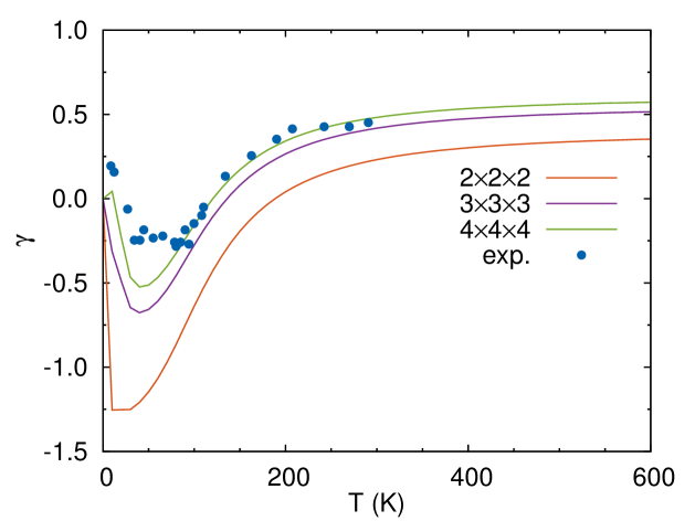
Figure 1: Average Grüneisen parameter for three different super-cell sizes for Si. Circles represent experimental values [42].

2.2.3 Distorted volume single point calculations

To obtain $F(V,T)$ vs. $V(T)$ curves, phonon calculations have been performed for thirteen equally spaced configurations in which the volume of cell was compressed and expanded in the range from 98 $\%$ to 113 $\%$ of its fully relaxed value. $F_{elec}(V,T)$ is computed from static and band calculations of the expanded and compressed primitive cells following AFLOW standard [21] that are consistent with the setup used for the geometry optimizations.

There are limitations derived by the level of theory or functional. PBE could predict metallic behavior in semiconductors with a narrow band gap. This error would modify $F_{elec}(V,T)$ which is a small contribution at low and moderate temperatures. To verify that none of the materials included in the data set present this anomaly, we have compared the calculated band gaps with the experimental values (see Table 1 in Supplementary Information).

2.3 Analysis of Results

Different statistical parameters have been used to measure the qualitative and quantitative agreement of QHA-APL with experimental values. The Pearson correlation coefficient $r$ is a measure of the linear correlation between two variables, $X$ and $Y$. It is calculated by

$$r=\frac{\sum_{i=1}^{n}\left(X_{i}-\overline{X}\right)\left(Y_{i}-\overline{Y}\right)}{\sqrt{\sum_{i=1}^{n}\left(X_{i}-\overline{X}\right)^{2}}\sqrt{\sum_{i=1}^{n}\left(Y_{i}-\overline{Y}\right)^{2}}},$$ (12)

where $\overline{X}$ and $\overline{Y}$ are the mean values of $X$ and $Y$.

The Spearman rank correlation coefficient $\rho$ is a measure of the monotonicity of the relationship between two variables. The values of the two variables $X_{i}$ and $Y_{i}$ are sorted in ascending order, and are assigned rank values $x_{i}$ and $y_{i}$ which are equal to their position in the sorted list. The correlation coefficient is then given by

$$\rho=\frac{\sum_{i=1}^{n}\left(x_{i}-\overline{x}\right)\left(y_{i}-\overline{y}\right)}{\sqrt{\sum_{i=1}^{n}\left(x_{i}-\overline{x}\right)^{2}}\sqrt{\sum_{i=1}^{n}\left(y_{i}-\overline{y}\right)^{2}}}.$$ (13)

It is useful for determining how well the ranking order of the values of one variable predict the ranking order of the values of the other variable.

We also investigate the root-mean-square relative deviation ($RMSrD$) of the calculated results from experiment. This gives a measure of the magnitude of the difference between the QHA-APL predictions and experiment. The root mean square relative deviation ($RMSrD$) is calculated using the expression

$$RMSrD=\sqrt{\frac{\sum_{i=1}^{n}\left(\frac{X_{i}-Y_{i}}{X_{i}}\right)^{2}}{N-1}},$$ (14)

Note that lower values of the $RMSrD$ indicate better agreement with experiment.

3 Results

A benchmark of 130 materials has been used to demonstrate the accuracy and robustness of this method (see Table LABEL:tab:data). To maximize the heterogeneity of the data set, these compounds were selected to belong to different crystallographic lattices (cubic, tetragonal, orthorhombic, hexagonal, rhombohedral and monoclinic) as well as different electronic properties (insulators, semiconductors and metals, see Supplementary Information for the computed and experimental energy gaps).

Table 1: ICSD identification number, Bulk modulus ($B$), Grüneisen parameter ($\gamma$), Volumetric thermal expansion coefficient ($\alpha$), and Isochoric specific heat ($C_{p}$) for material data set. Experimental values in parenthesis. Units: $B$ in GPa, $\alpha$ in 10^-6K^-1, and $C_{p}$ in Jmol^-1K^-1 (see Supplementary Information for the computed and experimental energy gaps).

Formula	ICSD	$B$	$\gamma$	$\alpha$	Cp	Formula	ICSD	$B$	$\gamma$	$\alpha$	Cp
Ag1Cl1	157535	28.6(44.0)[43]	2.30	114.0	53.5(53.0)[44]	Ge1	44841	55.1(78.0)[45]	0.74(0.76)[46]	21.5(16.2)[47]	23.3(23.3)[44]
Ag1Mg1	184205	48.6	2.14	89.2	50.5	Ge1Mg2	81735	46.63	1.46	53.8	71.2
Ag1Sc1	58348	65.8	1.66	46.6	49.3	H1Li1	61751	32.0(33.7)[48]	1.10(1.28)[46]	87.1	27.6(28.1)[44]
Ag3Mg1	58323	58.1	2.41	86.9	102.7	H1Li1Pd1	246613	77.5	1.71	63.4	17.7
Al1As1	606008	64.5(77.0)[49]	0.57(0.66)[46]	13.7	44.4(45.8)[44]	H1Mg1Ni1	187257	86.3	1.21	40.1	55.1
Al1B2	159334	167.5	1.16	22.2	51.0(43.9)	H1Na1	183291	18.8	0.79	78.9	34.8(36.5)
Al1	240129	67.5	2.41	80.8(69.0)[47]	24.3(24.2)[47]	H1Ti1	168325	112.8	0.88	15.8	26.4
Al1Li1	240121	47.6	1.54	69.1	44.5(48.9)[44]	Hg1Ni1	639119	104.8	2.82	68.2	51.3
Al1N1	602459	188.0(201.0)[50]	0.80(0.70)[51]	10.1	31.0(30.1)[44]	Hg1Pd1	639137	101.0	3.10	67.2	52.0
Al1Ni1	608805	147.1	1.93	40.5	45.9(45.9)[44]	Hg1Pt1	104337	127.4	3.28	57.0	51.8
Al1P1	609019	80.6(86.0)[49]	0.50(0.75)[51]	10.3	41.5(42.0)[44]	Hg1Zr1	639318	97.6	2.19	41.3	49.9
Al1Sb1	609290	47.3(58.2)[45]	0.44(0.60)[46]	11.7(12.6)[47]	45.8	I1K1	53827	8.3(11.1)[52]	1.77(1.45)[46]	178.6(122.4)[53]	54.0(52.80)[53]
Al1Sc1	58098	63.6	1.83	52.9	47.0	I1Li1	27983	9.7	2.93	395.9(178.2)[53]	65.1
Al1Si1Sr1	162865	51.9	1.31	37.7	69.3	I1Na1	52240	14.0(15.95)[52]	1.94(1.56)[46]	156.0(136.5)[53]	53.5(52.26)[53]
Al1Tb3	58173	45.9	0.51	16.2	96.5	I1Rb1	53846	7.1(11.1)[52]	1.54(1.41)[46]	161.6(124.5)[53]	53.3(52.5)[44]
Al1Ti1	187030	92.1	1.54	35.6	45.6(49.3)[44]	In1N1	157515	118.5(126.0)[54]	0.82(0.97)[55]	14.3	40.0
Al3Ti1	609525	97.9	1.49	33.8	89.7	In1P1	165466	56.5(71.0)[49]	0.62(0.60)[46]	15.7(13.8)[47]	45.6(45.5)[44]
As1B1	181292	126.6	0.80	13.0	34.9	In1Te1	169431	34.0	2.57	96.1	52.9(47.7)[44]
As1Ba1Li1	56445	31.1	1.27	55.7	70.9	In1Te1	640622	32.3	2.57	101.1	53.1(47.7)[44]
As1Ga1	53964	57.2(74.8)[49]	0.76(0.75)[46]	21.6(16.2)[47]	46.9(46.8)[44]	K1	641218	2.6(3.1)	0.80	158.2	25.7(29.4)[44]
As1In1	165462	43.6(58.0)[49]	0.64(0.57)[46]	19.7(14.1)[47]	43.6(47.8)[44]	K2O1	44674	45.1	1.76	73.7	73.7
B1Sb1	184571	94.9	0.85	15.2	38.0	K2S1	183837	35.9	1.54	50.0	74.3
B2Ti1	78847	231.4	1.27	15.3	45.7	Li1Pd1	642257	52.5	1.62	80.9	45.5
B2V1	167794	265.9	1.35	15.8	45.8	Li1Pt1	104777	110.2	1.44	34.1	44.5
Be1	52708	99.4	1.63	54.2	16.5(16.52)[44]	Li2O1	60431	72.8(88.0)	1.19	55.1	53.9
Be1Rh1	58734	210.0	2.10	32.5	43.1	Li2S1	657596	31.3	1.22	83.3	64.4
Be1S1	186889	89.7(105.0)[56]	0.91	20.9	36.7(34.2)[44]	Li2Se1	168446	28.4	1.04	70.7	66.8
Be1Se1	616419	70.8(92.0)[56]	0.80	21.1	39.9	Li2Te1	642399	24.0	1.06	69.4	69.0
Be1Te1	290008	53.8(67.0)[56]	0.72	19.9	41.6	Mg1O1	159372	147.3(164)[57]	1.53(1.44)[46]	33.3	38.3(37.2)[44]
Be2C1	616184	179.3	1.17	20.2	38.9(43.3)[44]	Mg1Pt3	104857	164.1	2.70	40.1	98.4
Bi1Na1	616837	24.1	1.92	106.8	51.9	Mg1S1	53939	68.1	1.68	50.7	46.4(45.6)[44]
Br1Cu1	30090	36.8	1.19	53.5(46.2)[47]	49.5(54.8)[44]	Mg1Sc1	108583	48.1	1.56	51.3	47.8
Br1K1	52243	11.0(15.4)[52]	1.87(1.45)[46]	170.5(116.1)[53]	53.7(52.3)[53]	Mg1Se1	159398	53.3	0.27	71.8	46.2 (48.0)
Br1Li1	53819	19.4(26.0)[52]	2.39	216.6(149.4)[53]	54.9(48.9)[53]	Mg2Pb1	104846	29.9	1.27	59.4	73.1(72.5)[44]
Br1Na1	44278	16.0(19.6)[52]	1.69(1.5)[46]	148.0(126.9)[53]	52.3(51.9)[53]	Mg2Si1	163708	17.0	1.22	44.3(34.5)[47]	68.7(68.0)[44]
C1	182729	416.9(442.0)[45]	0.73(0.75)[46]	3.2(3.5)[47]	6.4 (8.6)[44]	Mg2Sn1	151368	37.8	1.30	50.0(29.7)[47]	72.3
C1Si1	618777	211.0(211.0)[45]	0.72(0.75)[46]	7.3	27.7(27.1)[44]	Mn1O1	18006	136.3	1.78	39.9	44.1(44.17)[44]
C1Ti1	181681	230.0	1.44	16.8	35.1(33.9)[44]	Mn1S1	76205	52.9	0.42	12.8	45.9(45.6)[44]
C1Zr1	180599	212.0	1.58	17.9	38.7	Mn1Se1	24252	45.0	0.30	9.7	47.6(51.0)[44]
Ca1Cd1	619188	27.3	1.57	78.6	50.4	Mn1Te1	181324	68.9	0.23	7.9	48.3
Ca1F2	40938	68.3(84.0)	1.78	68.7	68.7(68.7)[44]	N1Sc1	155049	179.2	1.57	22.7	38.6
Ca1O1	180198	98.6(113)[58]	1.57(1.57)[46]	39.3	43.4(42.2)[44]	N1Ti1	183415	248.3	1.71	21.0	37.6(37.2)[44]
Ca1S1	619530	69.6	1.46	34.1	47.0(47.4)[44]	Na1	644903	6.7	1.32	20.3	26.4
Ca1Se1	619570	46.0	1.50	47.8	48.8(48.1)[44]	Se1Zn1	181761	53.3	0.83	26.4	47.8
Ca1Te1	619616	34.6	1.47	51.3	49.5(41.6)[44]	Ni1O1	166115	168.9	1.59	33.6	42.1(44.5)[44]
Cd1F2	28864	79.3	2.20	74.1	71.2	Ni1Sb1	646431	107.3	1.73	36.2	48.6
Cd1O1	181735	114.4	1.94	46.0	46.1(43.7)[44]	Ni1Sc1	105333	96.2	1.86	45.6	48.7
Cd1Pd1	620270	91.6	2.32	57.1	50.4	Ni1Zn1	647134	129.5	1.86	46.8	48.1
Cd1Pt1	620297	119.3	2.70	51.7	50.7	Ni2Sn1Ti1	646777	138.5	2.17	41.3	97.2(98.0)[44]
Cd1S1	290009	46.8	0.53(0.75)[51]	16.8	46.7	O1Pd1	26598	142.3	1.51	19.8	39.1
Cd1Sr1	102066	19.8	1.51	89.0	51.3	O1Sr1	26960	76.4(91.2)[58]	1.63(1.52)[46]	44.8	46.2(45.4)[44]
Cd3Zr1	102093	71.8	1.99	50.5	100.2	O1Zn1	182356	121.0	0.66(0.75)[51]	15.7	40.3(41.17)[44]
Cl1Cu1	78270	35.6	0.86	46.2(36.3)[47]	48.3(52.6)[44]	O1Zn1	647683	121.4(143)[45]	0.66	15.7	40.3
Cl1K1	240522	13.3(18.2)[52]	1.77(1.45)[46]	157.4(111.3)[53]	52.7(51.7)[53]	Pd1Zn1	649134	115.0	2.43	58.4	50.0
Cl1Li1	26909	38.9(32.9)[52]	2.71	119.6(131.4)[53]	50.0(48.1)[53]	Pt1Zn1	105852	159.4	2.13	37.6	49.2
Cl1Na1	240600	19.7(25.1)[52]	1.75(1.56)[46]	145.7(119.1)[53]	51.6(50.54)[53]	S1Zn1	108733	65.6(71.4)[49]	0.79(0.75)[46]	23.1	45.5
Cl1Rb1	18016	10.2(16.2)[52]	1.55(1.45)[46]	156.5(108.0)[53]	52.6(52.3)[53]	Sc1	164093	52.1	1.10	30.8	23.8(25.58)[44]
Cu1I1	163427	18.9	1.36	101.0	51.0	Sc1Zn1	106041	65.1	1.39	42.3	48.3
Cu1	627117	114.5	1.91	53.5	24.3(24.5)[44]	Si1	76268	84.9(100.0)[45]	0.42(0.56)[51]	8.0(7.8)[47]	20.0(20.0)[44]
Cu1Sn1	629278	54.7	2.40	85.4	51.9	Tc1V1	106143	232.5	1.91	21.7	45.9
Cu2Ni1Zn1	103079	124.7	1.93	50.5	96.7	Te1Zn1	184485	39.4(51.0)[49]	0.89(0.97)[46]	30.7	48.6
F1K1	52241	22.5(31.6)[52]	1.59(1.5)[46]	133.4(104.4)[53]	50.5(49.0)[53]	Te1Zr1	653209	93.1	1.60	27.6	48.2
F1Li1	53839	55.8(76.0)[52]	1.63(1.5)[46]	109.9(99.6)[53]	42.8(42.0)[53]	Ti1	168830	109.3	1.62	30.1	23.5(25.1)[44]
F1Na1	52238	37.3(48.5)[52]	1.52(1.5)[46]	113.7(95.1)[53]	47.8(46.9)[53]	Zn1	181734	44.8	2.47	144.8	26.8(25.41)[44]
Ga1P1	77088	74.8(88.7)[49]	0.70(0.75)[46]	16.2(15.9)[47]	44.1(44.2)[44]	Zn1Zr1	181290	96.3	1.42	31.2	48.3
Ga1Sb1	41675	42.7(45.1)[49]	0.71(0.75)[46]	21.9	47.9

For each temperature, we calculated the free energy ($F$) at different volumes (V). These $F$ vs. $V$ curves are initially fitted to a cubic function which is used as an initial guess to fit the Birch-Murnaghan equation of state (see “Method” and Eq. 6). As an example, the results of the final fitting for Si are depicted in Fig. 2. Automatic tests to ensure the correct fitting of the curves have been implemented to warn of possible errors, especially in magnetic systems or close to phase transition temperatures. The bulk modulus, $B$, at 300 K is obtained by the fitting procedure. Fig. 3 (a) illustrates the distribution of $B$ for the whole set of materials while Fig. 3 (b) compares experimental and predicted values of $B$ for those materials with available experimental data. The computed values range over two orders of magnitude, from C diamond (442 GPa) to K (3.2 GPa). To quantify the accuracy, precision and robustness of our results we have used different statistical quantities such as mean absolute deviation (MAD), root mean square deviation (RMSD), root mean square relative deviation (RMSrD), relative maximum absolute deviation (rMAX), and Pearson and Spearman correlation (see Table 2). Most of the predicted values are within a 20% error (dashed lines in Fig. 3 (b)), presenting a RMSrD of around 17% and a rMAX close to 22.9%. Values close to 1.0 for the Pearson and Spearman correlations also demonstrate that our implementation of the QHA is robust and that the results can be compared with experimental data.

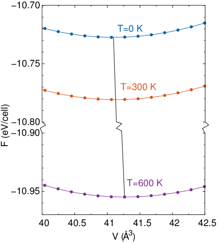
Figure 2: Free energy and volume data fitted using Birch-Murnaghan function for different temperatures for Si. Points represent calculated data and solid lines indicate the fitted function. Equilibrium volumes at each temperature are connected by solid black line.

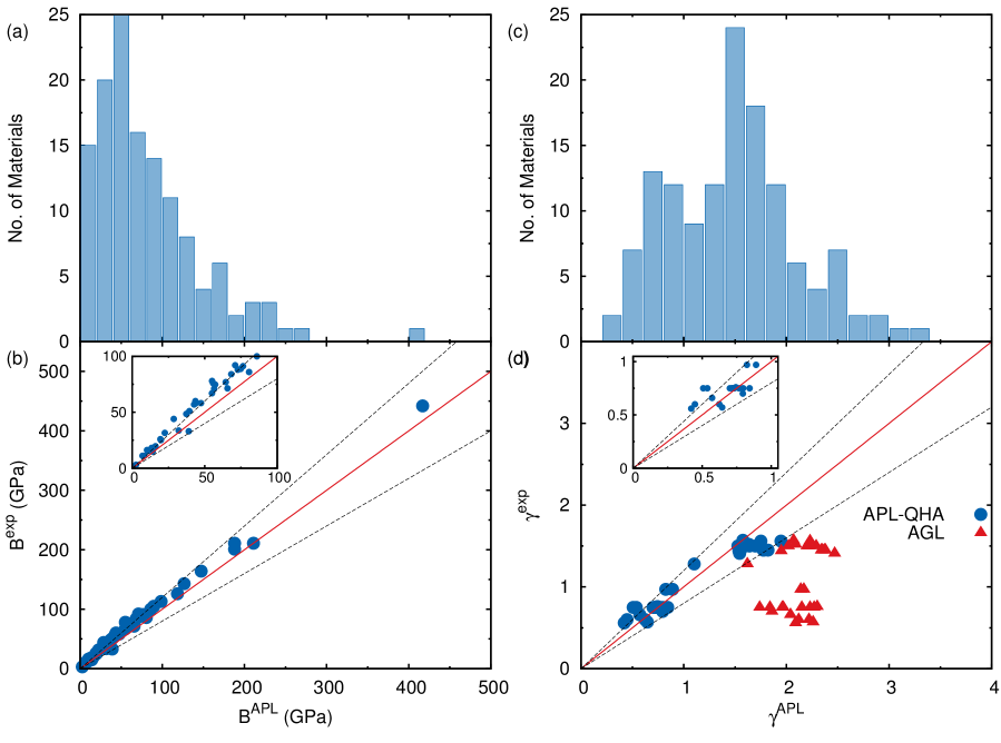
Figure 3: (a) Histogram for the dispersion of predicted $B$ at 300 K for the selected set of systems. (b) Comparison of experimental $B^{exp}$ and predicted $B^{APL}$ for the selected set of systems. The red line represents equality between experimental and predicted values and the dashed black lines represent $\pm$20% error. (c) Histogram for the dispersion of predicted Grüneisen parameters at 300 K for the selected set of systems. (d) Comparison of experimental $\gamma^{exp}$ and predicted $\gamma^{APL}$ for the selected set of systems. Ther red line represents equality between experimental and predicted values and the dashed black lines represent $\pm$20% error. The blue circles represent QHA-APL results and the red triangles correspond to AGL results [3].

Table 2: Mean absolute deviation (MAD), root mean square deviation (RMSD), root mean square relative deviation (RMSrD), relative maximum absolute deviation (rMAX), and Pearson and Spearman correlation for the material data set. Units: MAD and RMSD in the same units that are used in Table LABEL:tab:data

	$B$	$\gamma$	$\alpha$	$C_{p}$
MAD	11.09	0.13	20.22	1.63
RMSD	12.89	0.17	28.15	2.45
RMSrD	17.38%	15.00%	28.0%	6.35%
rMAX	22.9%	28.32%	46.5%	18.9%
$r$	0.996	0.969	0.974	0.985
$\rho$	0.990	0.891	0.927	0.929

In the spirit of the QHA, the Grüneisen parameter, $\gamma(T)$, is often used to estimate the anharmonicity of the vibrations in the crystal. Methods such as AGL are able to predict reasonably accurate values for the Debye temperature or $B$ but fail to predict $\gamma(T)$ [3]. Our QHA-APL results are shown in Fig. 3 which includes, for comparison, the available results using AGL for the same compounds. Despite the higher computational cost of the QHA compared to the AGL methodology (one or two orders of magnitude higher than AGL depending on the size of the system), it is clear that results are tremendously improved. The MAD for QHA-APL is 0.13 for a property whose highest measured value is around 3 and the average values are between 1 and 2. Relative statistical indicators also demonstrate the high accuracy of the method obtaining a RMSrD below 16% and a rMAX lower than 29%. Values larger than 3 are especially interesting for their potential application as thermoelectrics. As we mentioned, $\gamma(T)$ is related to the anharmonicity of the crystal, so high values for this property usually [59] indicate lower values of the lattice thermal conductivity, $\kappa_{L}$, which increases the thermoelectric figure of merit, $ZT$. We have found two materials with $\gamma$ over 3, however both are metals (HgPd, HgPt). We have looked for other possible candidates with high values of $\gamma$ considering also that for a high thermoelectric figure of merit they should be semiconductors. K₂O and MnO are the best two candidates, with $\gamma$ around 1.8 and band gaps below 2 eV. There is no experimental data available for K₂O, although Gheribi et al. have predicted a lattice thermal conductivity for this material below 2 Wm^-1K^-1 [60].

The Grüneisen parameters for each vibrational mode, $\gamma_{iq}$, provide even more information than $\gamma$ about the anharmonicity of the crystal and the lattice thermal conductivity. High and low values of $\kappa_{L}$ in an insulator are usually linked to low and high values of $\gamma_{iq}$ at low frequency. SiC ($\kappa$=360 Wm^-1K^-1) [51] and NaI ($\kappa$=1.8 Wm^-1K^-1) [51] are two good examples of this trend (see Fig. 4 (a) and (b)) that has been exploited in the literature to pinpoint anharmonic effects [61, 62]. We have studied the mode Grüneisen parameters of two other materials included in the benchmark whose $\kappa_{L}$ has not been measured experimentally. We have already discussed the probable low thermal conductivity of K2O which is in agreement with the very high mode Grüneisen parameter values at low frequencies (see Fig. 4 (d)). BeTe shows the opposite behavior to K2O, presenting low values for $\gamma_{iq}$ at low frequencies (see Fig. 4 (c)). This trend is in agreement with the AGL prediction of $\kappa_{L}$ for BeTe, which is close to the value obtained for AlAs ($\kappa$=98 Wm^-1K^-1) [51]. These predictions validate the use of $\gamma$ and $\gamma_{iq}$ as a simple predictors for $\kappa_{L}$ and demonstrates that the QHA-APL method can be used as a powerful method for the discovery of new interesting properties in well known materials.

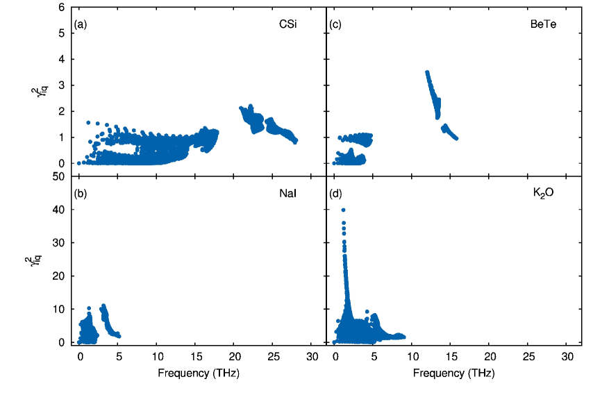
Figure 4: Mode Grüneisen parameters for (a) SiC, (b) NaI, (c) BeTe, and (d) K2O.

The volumetric thermal expansion, $\alpha_{V}(T)$, has very important implications in engineering. However, it is not easy to predict accurately from first principles. Statistical parameters prove again that QHA-APL methodology is a reliable method to obtain this thermodynamic quantity. The uncertainty as described by RMSrD is below 28% and MAD is around 20.22 10^-6K^-1 for the benchmark in which the range varies between 0 and 160 10^-6K^-1. Low thermal expansion coefficient materials deserve special attention because they are particularly interesting for a variety of applications. There are 5 materials in our benchmark that present a value of $\alpha$ below 10^-5K^-1 (see Fig. 5 (b)). Three of them have been already reported, C, Si and CSi. However, to the best of our knowledge, the other two materials have not been experimentally measured or predicted: MnTe and MgSe.

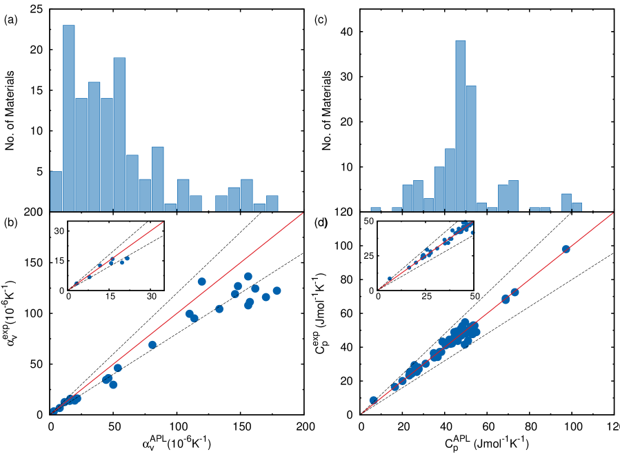
Figure 5: (a) Histogram for the dispersion of predicted volumetric thermal expansion coefficient at 300 K for the selected set of systems. (b) Comparison of experimental $\alpha^{exp}$ and predicted $\alpha^{APL}$ for the selected set of systems. The red line represents equality between experimental and predicted values and the dashed black lines represent $\pm$20% error. (c) Histogram for the dispersion of predicted isobaric specific heat at 300 K for the selected set of systems. (d) Comparison of experimental $C_{p}^{exp}$ and predicted $C_{p}^{APL}$ for the selected set of systems. The red line represents equality between experimental and predicted values and the dashed black lines represent $\pm$20% error.

Isobaric specific heat, $C_{p}$, can be considered another good test for our method because of the vast amount of available experimental data (see Fig. 5 (d)). The low MAD (9.84 Jmol^-1K^-1) is surprising for a property in which the average value of our data set is close to 50 Jmol^-1K^-1. This fact is also reflected in the relative statistical parameters (RMSrD = 6.35% and rMAX = 18.9%) and correlations close to 1.0. A caveat should be mentioned: this deviation grows slightly when comparing $C_{p}$ at 1000 K instead of 300 K. This is due to higher anharmonicity at higher temperatures.

Some groups of materials are more likely to show larger deviations because of the exchange-correlation functional limitations. Inaccurate band gaps could lead to predict metallic behavior in semiconductor with a narrow band gap. This qualitative disagreement can modify the electronic terms in the free energy. To ensure that our description is correct, we have calculated the RMSrD for metals and semiconductors with a predicted band gap smaller than 1.0 eV. For metals, the RMSrD is 8.1% for $C_{p}$, which is below the RMSrD for the whole data set. We have also calculated this quantity for $\alpha_{V}(T)$ and $C_{p}$ for low band gap semiconductors, obtaining 30.0% and 3.6% respectively. Both values are also close to the RMSrD obtained for the whole data set. Despite QHA limitations, we demonstrate that our implementation can predict the properties of different groups of materials.

We also computed the temperature dependence for selected materials in the data set (see Fig. 6). Our implementation predicts correctly the behavior of $\gamma(T)$, $B$, $\alpha_{V}(T)$ and $C_{p}$ below melting points for various types of materials (metals, insulators and semiconductors). The bulk modulus for insulators such as NaCl and KCl are shown in Fig. 6 (a) with errors smaller than 25%. QHA-APL also predicts $\alpha_{V}(T)$ for complex metals as Ni2SnTi with a high accuracy below its melting point (see Fig. 6 (b)). Finally, $C_{p}$ for GaAs, a classic semiconductor, is depicted in Fig. 6 (c) presenting errors smaller than 2%.

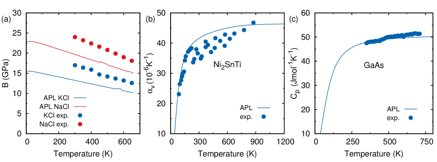
Figure 6: (a) Predicted bulk modulus of NaCl and KCl compared to the available experimental data [63]. (b) Predicted volumetric thermal expansion coefficient of Ni2SnTi compared to the available experimental data [64]. (c) Predicted isobaric specific heat of GaAs compared to the available experimental data [65].

More sophisticated electronic structure methods can be used to validate our data. Our framework can use different exchange correlation functionals such as the pseudo hybrid functional ACBN0 [33]. We have used K2O as a test to study how a more accurate functional works compared to the results obtained with PBE (see Fig. 7). Despite the use of a more accurate approach, the band gap (1.8 eV compared to 1.71 eV for PBE), phonon dispersion curves and the average Grüneisen parameter for K2O are only slightly modified by ACBN0.

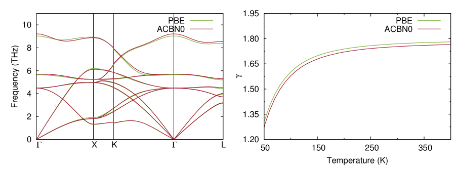
Figure 7: (a) Phonon dispersion curves and (b) average Grüneisen parameter for K2O using PBE and ACBN0 functionals.

4 Conclusions

The quasi-harmonic approximation has been combined with the Automatic Phonon Library in the AFLOW high-throughput framework in order to develop a tool to accurately and robustly predict some of the most important temperature dependent properties of solids such as $B$, $\gamma$, $\alpha$, and $C_{p}$. Lattice dynamics calculations at different volumes for fully relaxed structures are performed, managed, self-corrected, and post processed by the QHA-APL code, creating a unique workflow to populate material databases such as AFLOW. A benchmark of 130 materials has been used to test the precision and accuracy of the software. QHA-APL predicts results whose RMSrD is below 18% for any of the four quantities with respect to experimentally reported data. We confirm recent results on K2O and computed data for well known materials that have not been reported before. QHA-APL is useful not just for the prediction of properties for particular materials; its automation, robustness, accuracy and precision make it the perfect framework for the creation of material data sets that can be used for data mining or machine learning.

5 Acknowledgements

We thank Dr. E. Perim, Dr. O. Levy, A. Supka, and M. Damian for various technical discussions. We would like to acknowledge support by DOD-ONR (N00014-13-1-0635, N00014-11-1-0136, N00014-09-1-0921) and by DOE (DE-AC02- 05CH11231), specifically the BES program under Grant # EDCBEE. The AFLOW consortium would like to acknowledge the Duke University - Center for Materials Genomics and the CRAY corporation for computational support.

References

- Curtarolo et al. [2013] S. Curtarolo, G. L. W. Hart, M. Buongiorno Nardelli, N. Mingo, S. Sanvito, O. Levy, The high-throughput highway to computational materials design, Nat. Mater. 12 (2013) 191–201, doi:10.1038/nmat3568.
- Blanco et al. [2004] M. A. Blanco, E. Francisco, V. Luaña, GIBBS: isothermal-isobaric thermodynamics of solids from energy curves using a quasi-harmonic Debye model, Computer Physics Communications 158 (1) (2004) 57–72, doi:10.1016/j.comphy.2003.12.001.
- Toher et al. [2014] C. Toher, J. J. Plata, O. Levy, M. de Jong, M. D. Asta, M. Buongiorno Nardelli, S. Curtarolo, High-Throughput Computational Screening of thermal conductivity, Debye temperature and Grüneisen parameter using a quasi-harmonic Debye Model, Phys. Rev. B 90 (2014) 174107, doi:10.1103/PhysRevB.90.174107.
- Li et al. [2014] W. Li, J. Carrete, N. A. Katcho, N. Mingo, ShengBTE: a solver of the Boltzmann transport equation for phonons, Comput. Phys. Commun. 185 (2014) 1747–1758, doi:10.1016/j.cpc.2014.02.015.
- Togo et al. [2015] A. Togo, L. Chaput, I. Tanaka, Distributions of phonon lifetimes in Brillouin zones, Phys. Rev. B 91 (2015) 094306, doi:10.1103/PhysRevB.91.094306.
- Plata et al. [2016] J. J. Plata, P. Nath, D. Usanmaz, J. Carrete, T. Toher, M. Fornari, M. B. Nardelli, S. Curtarolo, APL 2.0: An automatic high throughput phonon calculator for finite temperature properties, In preparation .
- Ho and Taylor [1998] C. Y. Ho, R. E. Taylor (Eds.), Thermal Expansion of Solids, Asm. Intl., 1998.
- Baroni et al. [2010] S. Baroni, P. Giannozzi, E. Isaev, Density-Functional Perturbation Theory for Quasi-Harmonic Calculations, Rev. Mineral Geochem. 71 (2010) 39–57, doi:10.2138/rmg.2010.71.3.
- Carrier et al. [2007] P. Carrier, R. Wentzcovitch, J. Tsuchiya, First-principles prediction of crystal structures at high temperatures using the quasiharmonic approximation, Phys. Rev. B 76 (2007) 064116, doi:10.1103/PhysRevB.76.064116.
- Alfé [2009] D. Alfé, PHON: A program to calculate phonons using the small displacement method, Comput. Phys. Commun. 180 (2009) 2622–2633, doi:10.1016/j.cpc.2009.03.010.
- Duong et al. [2011] T. Duong, S. Gibbons, R. Kinra, R. Arroyave, Ab-initio aprroach to the electronic, structural, elastic, and finite-temperature thermodynamic properties of Ti2AX (A = Al or Ga and X = C or N), J. Appl. Phys. 110 (2011) 093504, doi:http://dx.doi.org/10.1063/1.3652768.
- Wang et al. [2014] J. Wang, J. Wang, A. Li, J. Li, Y. Zhou, Theoretical Study on the Mechanism of Anisotropic Thermal Properties of Ti2AlC and Cr2AlC, J. Am. Ceramic. Soc. 97 (2014) 1202–1208, doi:10.1111/jace.12814.
- Huang et al. [2016] L. F. Huang, X. Z. Lu, E. Tennessen, J. M. Rondinelli, An efficient ab-initio quasiharmonic approach for the thermodynamics of solids, Comput. Phys. Commun. 120 (2016) 84–96, doi:10.1016/j.commatsci.2016.04.012.
- Togo and Tanaka [2015] A. Togo, I. Tanaka, First principles phonon calculations in materials science, Scr. Mater. 108 (2015) 1–5, doi:10.1016/j.scriptamat.2015.07.021.
- Curtarolo et al. [2012a] S. Curtarolo, W. Setyawan, G. L. W. Hart, M. Jahnátek, R. V. Chepulskii, R. H. Taylor, S. Wang, J. Xue, K. Yang, O. Levy, M. J. Mehl, H. T. Stokes, D. O. Demchenko, D. Morgan, AFLOW: An automatic framework for high-throughput materials discovery, Comp. Mat. Sci. 58 (2012a) 218–226, doi:10.1016/j.commatsci.2012.02.005.
- Jahnátek et al. [2011] M. Jahnátek, O. Levy, G. L. W. Hart, L. J. Nelson, R. V. Chepulskii, J. Xue, S. Curtarolo, Ordered phases in ruthenium binary alloys from high-throughput first-principles calculations, Phys. Rev. B 84 (2011) 214110, doi:10.1103/PhysRevB.84.214110.
- Chaput et al. [2011] L. Chaput, A. Togo, I. Tanaka, G. Hug, Phonon-phonon interactions in transition metals, Phys. Rev. B 84 (2011) 094302, doi:10.1103/PhysRevB.84.094302.
- Tadano et al. [2014] T. Tadano, Y. Gohda, S. Tsuneyuki, Anharmonic force constants extracted from first-principles molecular dynamics: applications to heat transfer simulations, J. Phys.: Conden. Matt. 26 (2014) 225402, doi:10.1088/0953-8984/26/22/225402.
- Curtarolo et al. [2012b] S. Curtarolo, W. Setyawan, S. Wang, J. Xue, K. Yang, R. H. Taylor, L. J. Nelson, G. L. W. Hart, S. Sanvito, M. Buongiorno Nardelli, N. Mingo, O. Levy, AFLOWLIB.ORG: A distributed materials properties repository from high-throughput ab initio calculations, Comp. Mat. Sci. 58 (2012b) 227–235, doi:10.1016/j.commatsci.2012.02.002.
- Taylor et al. [2014] R. H. Taylor, F. Rose, C. Toher, O. Levy, K. Yang, M. Buongiorno Nardelli, S. Curtarolo, A RESTful API for exchanging Materials Data in the AFLOWLIB.org consortium, Comp. Mat. Sci. 93 (2014) 178–192, doi:10.1016/j.commatsci.2014.05.014.
- Calderon et al. [2015] C. E. Calderon, J. J. Plata, C. Toher, C. Oses, O. Levy, M. Fornari, A. Natan, M. J. Mehl, G. L. W. Hart, M. Buongiorno Nardelli, S. Curtarolo, The AFLOW Standard for High-Throughput Materials Science Calculations, Comp. Mat. Sci. 108 Part A (2015) 233–238, doi:10.1016/j.commatsci.2015.07.019.
- Orlikowski et al. [2006] D. Orlikowski, P. Söderlind, J. A. Moriarty, First-principles thermoelasticity of transition metals at high pressure: Tantalum prototype in the quasiharmonic limit, Phys. Rev. B 74 (2006) 054109, doi:10.1103/PhysRevB.74.054109.
- Xiang et al. [2010] S. Xiang, F. Xi, Y. Bi, J. Xu, H. Geng, L. Cai, F. Jing, J. Liu, Ab initio thermodynamics beyond the quasiharmonic approximation: W as a prototype, Phys. Rev. B 81 (2010) 014301, doi:10.1103/PhysRevB.81.014301.
- Grabowski et al. [2009] B. Grabowski, L. Ismer, T. Hickel, J. Neugebauer, Ab initio up to the melting point: Anharmonicity and vacancies in aluminum, Phys. Rev. B 79 (13) (2009) 134106, doi:10.1103/PhysRevB.79.134106.
- Skelton et al. [2014] J. M. Skelton, S. C. Parker, A. Togo, I. Tanaka, A. Walsh, Thermal physics of the lead chalcogenides PbS, PbSe, and PbTe from first principles, Phys. Rev. B 89 (2014) 205203, doi:10.1103/PhysRevB.89.205203.
- Iikubo et al. [2010] S. Iikubo, H. Ohtani, M. Hasebe, First-Principles Calculations of the Specific Heats of Cubic Carbides and Nitrides, Mater. Trans. 51 (2010) 574–577, doi:10.2320/matertrans.MBW200913.
- de-la Roza and Luaña [2011] A. O. de-la Roza, V. Luaña, Treatment of first-principles data for predictive quasiharmonic thermodynamics of solids: The case of MgO, Phys. Rev. B 84 (2011) 024109, doi:10.1103/PhysRevB.84.024109.
- Tohei et al. [2015] T. Tohei, H.-S. Lee, Y. Ikuhara, First Principles Calculation of Thermal Expansion of Carbon and Boron Nitrides Based on Quasi-Harmonic Approximation, Mater. Trans. 56 (2015) 1452–1456, doi:10.2320/matertrans.MA201574.
- Kangarlou and Abdollahi [2014] H. Kangarlou, A. Abdollahi, Thermodynamic Properties of Copper in a Wide Range of Pressure and Temperature Within the Quasi-Harmonic Approximation, Int. J. Thermophys. 35 (2014) 1501–1511, doi:10.1007/s10765-014-1742-x.
- Burton et al. [2011] B. P. Burton, S. Demers, A. van de Walle, First principles phase diagram calculations for the wurtzite-structure quasibinary systems SiC-AlN, SiC-GaN and SiC-InN, J. Appl. Phys. 110 (2011) 023507, doi:10.1063/1.3602149.
- Golumbfskie et al. [2006] W. J. Golumbfskie, R. Arroyave, D. Shin, Z. K. Liu, Finite-temperature thermodynamic and vibrational properties of Al–Ni–Y compounds via first-principles calculations, Acta Mater. 54 (2006) 2291–2304, doi:http://dx.doi.org/10.1016/j.actamat.2006.01.013.
- Wee et al. [2012] D. Wee, B. Kozinsky, B. Pavan, M. Fornari, Quasiharmonic Vibrational Properties of TiNiSn from Ab Initio Phonons, J. Elec. Mat. 41 (2012) 977, doi:10.1007/s11664-011-1833-4.
- Agapito et al. [2015] L. A. Agapito, S. Curtarolo, M. Buongiorno Nardelli, Reformulation of as a Pseudohybrid Hubbard Density Functional for Accelerated Materials Discovery, Phys. Rev. X 5 (2015) 011006, doi:10.1103/PhysRevX.5.011006.
- Giannozzi et al. [2009] P. Giannozzi, S. Baroni, N. Bonini, M. Calandra, R. Car, C. Cavazzoni, D. Ceresoli, G. L. Chiarotti, M. Cococcioni, I. Dabo, A. Dal Corso, S. de Gironcoli, S. Fabris, G. Fratesi, R. Gebauer, U. Gerstmann, C. Gougoussis, A. Kokalj, M. Lazzeri, L. Martin-Samos, N. Marzari, F. Mauri, R. Mazzarello, S. Paolini, A. Pasquarello, L. Paulatto, C. Sbraccia, S. Scandolo, G. Sclauzero, A. P. Seitsonen, A. Smogunov, P. Umari, R. M. Wentzcovitch, QUANTUM ESPRESSO: a modular and open-source software project for quantum simulations of materials, J. Phys.: Conden. Matt. 21 (39) (2009) 395502.
- Kresse and Hafner [1993] G. Kresse, J. Hafner, Ab initio molecular dynamics for liquid metals, Phys. Rev. B 47 (1993) 558–561.
- Wallace [1972] D. C. Wallace, Thermodynamics of crystals, Wiley, 1972.
- Srivastava [1990] G. P. Srivastava, The Physics of Phonons, CRC Press, Taylor & Francis, 1990.
- Dove [1993] M. T. Dove, Introduction to Lattice Dynamics, Cambridge University Press, 1993.
- Blöchl [1994] P. E. Blöchl, Projector augmented-wave method, Phys. Rev. B 50 (1994) 17953–17979.
- Perdew et al. [1996] J. P. Perdew, K. Burke, M. Ernzerhof, Generalized gradient approximation made simple, Phys. Rev. Lett. 77 (1996) 3865–3868.
- Wang et al. [2010] Y. Wang, J. J. Wang, W. Y. Wang, Z. G. Mei, S. L. Shang, L. Q. Chen, Z. K. Liu, A mixed-space approach to first-principles calculations of phonon frequencies for polar materials, J. Phys.: Condens. Matter 22 (20) (2010) 202201, doi:10.1088/0953-8984/22/20/202201.
- B.Gauster [1971] W. B.Gauster, Low-Temperature Grüneisen Parameters for Silicon and Aluminum, Phys. Rev. B 4 (1971) 1288–1296, doi:10.1103/PhysRevB.4.1288.
- Hughes and Cain [1996] W. C. Hughes, L. S. Cain, Second-order elastic constants of AgCl from 20 to 430∘C, Phys. Rev. B 53 (1996) 5174, doi:http://dx.doi.org/10.1103/PhysRevB.53.5174.
- Barin [2008] I. Barin, Thermochemical Data of Pure Substances, WILEY-VCH, 2008.
- Madelung [2004] O. Madelung, Semiconductors: Data Handbook, Springer Berlin Heidelberg, Berlin, 2004.
- Slack [1979] G. A. Slack, The thermal conductivity of nonmetallic crystals, in: H. Ehrenreich, F. Seitz, D. Turnbull (Eds.), Solid State Physics, vol. 34, Academic, New York, 1, 1979.
- Lide [2004] D. R. Lide, CRC Handbook of Chemistry and Physics, Taylor & Francis, 2004.
- Laplaze et al. [1976] D. Laplaze, M. Boissier, R. Vacher, Velocity of hypersounds in lithium hydride by spontaneous Brillouin scattering, Solid State Commun. 19 (1976) 445–446, doi:10.1016/0038-1098(76)91187-X.
- Lam et al. [1987] P. K. Lam, M. L. Cohen, G. Martinez, Analytic relation between bulk moduli and lattice constants, Phys. Rev. B 35 (1987) 9190, doi:http://dx.doi.org/10.1103/PhysRevB.35.9190.
- McNeil et al. [1993] L. E. McNeil, M. Grimsditch, R. H. French, Vibrational Spectroscopy of Aluminum Nitride, J. Am. Ceramic. Soc. 76 (1993) 1132–1136, doi:10.1111/j.1151-2916.1993.tb03730.x.
- Morelli and Slack [2006] D. T. Morelli, G. A. Slack, High Lattice Thermal Conductivity Solids, in: S. L. Shindé, J. S. Goela (Eds.), High Thermal Conductivity Materials, Springer, 2006.
- Haussühl [1960] S. Haussühl, Thermo-elastische Konstanten der Alkalihalogenide vom NaCl-Typ, Z. für Physik 159 (1960) 223–229, doi:10.1007/BF01338349.
- Li [1976] H. H. Li, Refractive Index of alkali halides and its wavelength and temperature derivatives, J. Phys. Chem. Ref. Data 5 (1976) 329–528.
- Ueno et al. [1994] M. Ueno, M. Yoshida, A. Onodera, O. Shimomura, K. Takemura, Stability of the wurtzite-type structure under high pressure: GaN and InN, Phys. Rev. B 49 (1994) 14–21, doi:http://dx.doi.org/10.1103/PhysRevB.49.14.
- Krukowski et al. [1998] S. Krukowski, A. Witek, J. Adamczyk, J. Jun, M. Bockowski, I. Grzegory, B. Lucznik, G. Nowak, M. Wróblewski, A. Presz, S. Gierlotka, S. Stelmach, B. Palosz, S. Porowski, P. Zinn, Thermal properties of indium nitride, J. Phys. Chem. Solids 59 (3) (1998) 289–295, doi:10.1016/S0022-3697(97)00222-9.
- Xu et al. [2013] B. Xu, Q. Wang, Y. Tian, Bulk modulus for polar covalent crystals, Sci. Rep. 3 (2013) 3068, doi:10.1038/srep03068.
- Sumino et al. [1976] Y. Sumino, I. Ohno, T. Goto, M. Kumazawa, Measurement of elastic constants and internal frictions on single-crystal MgO by rectangular parallelepiped resonance, J. Phys. Earth 24 (1976) 263–273, doi:http://doi.org/10.4294/jpe1952.24.263.
- Chang and Graham [1977] Z. P. Chang, E. K. Graham, Elastic properties of oxides in the NaCl-structure, J. Phys. Chem. Solids 38 (1977) 1355–1362, doi:10.1016/0022-3697(77)90007-5.
- Carrete et al. [2014] J. Carrete, W. Li, N. Mingo, S. Wang, S. Curtarolo, Finding Unprecedentedly Low-Thermal-Conductivity Half-Heusler Semiconductors via High-Throughput Materials Modeling, Phys. Rev. X 4 (2014) 011019, doi:10.1103/PhysRevX.4.011019.
- Gheribi et al. [2015] A. E. Gheribi, A. Seifitokaldani, P. Wu, P. Chartrand, An ab initio method for the prediction of the lattice thermal transport properties of oxide systems: Case study of Li2O and K2O, J. Appl. Phys. 118 (2015) 145101, doi:10.1063/1.4932643.
- Orabi et al. [2016] R. A. R. A. Orabi, N. A. Mecholsky, J. Hwang, W. Kim, J.-S. Rhyee, D. Wee, M. Fornari, Band Degeneracy, Low Thermal Conductivity, and High Thermoelectric Figure of Merit in SnTe-CaTe, Chem. Mat. 28 (2016) 376–384, doi:DOI:10.1021/acs.chemmater.5b04365.
- Vaqueiro et al. [2015] P. Vaqueiro, R. A. R. A. Orabi, S. D. N. Luu, G. Guélou, A. V. Powell, R. I. Smith, J.-P. Song, D. Wee, M. Fornari, The role of copper in the thermal conductivity of thermoelectric oxychalcogenides: do lone pairs matter?, Phys. Chem. Chem. Phys. 17 (2015) 31735, doi:10.1039/C5CP06192J.
- Srivastava et al. [2009] S. K. Srivastava, P. Sinha, M. Panwar, Thermal expansivity and isothermal bulk modulus of ionic materials at high temperatures, Indian J. Pure Appl. Phys. 47 (2009) 175–179.
- Hermet et al. [2014] P. Hermet, R. M. Ayral, E. Theron, P. G. Yot, F. Salles, M. Tillard, P. Jund, Thermal Expansion of Ni-Ti-Sn Heusler and Half-Heusler Materials from First-Principles Calculations and Experiments, J. Phys. Chem. C 118 (39) (2014) 22405–22411, doi:10.1021/jp502112f.
- Blakemore [1982] J. S. Blakemore, Semiconducting and other major properties of gallium arsenide, J. Appl. Phys. 53 (1982) R123–R181, doi:10.1063/1.331665.