Solving generic nonarchimedean semidefinite programs
using stochastic game algorithms
Abstract.
A general issue in computational optimization is to develop combinatorial algorithms for semidefinite programming. We address this issue when the base field is nonarchimedean. We provide a solution for a class of semidefinite feasibility problems given by generic matrices. Our approach is based on tropical geometry. It relies on tropical spectrahedra, which are defined as the images by the valuation of nonarchimedean spectrahedra. We establish a correspondence between generic tropical spectrahedra and zero-sum stochastic games with perfect information. The latter have been well studied in algorithmic game theory. This allows us to solve nonarchimedean semidefinite feasibility problems using algorithms for stochastic games. These algorithms are of a combinatorial nature and work for large instances.
Key words and phrases:
Semidefinite programming, stochastic mean payoff games, nonarchimedean fields, tropical geometry2010 Mathematics Subject Classification:
90C22, 91A15, 12J25, 14T051. Introduction
Semidefinite programming consists in optimizing a linear function over a spectrahedron. The latter is a subset of defined by linear matrix inequalities, i.e., a set of the form
where the are symmetric matrices of order , and denotes the Loewner order on the space of symmetric matrices. By definition, if and only if is positive semidefinite.
Semidefinite programming is a fundamental tool in convex optimization. It is used to solve various applications from engineering sciences, and also to obtain approximate solutions or bounds for hard problems arising in combinatorial optimization and semialgebraic optimization. We refer the reader to [BPT13] and [GM12] for information.
Semidefinite programs are usually solved via interior point methods. The latter provide an approximate solution in a polynomial number of iterations, provided that a strictly feasible initial solution, i.e., a point belonging to the interior of the set , is known. We refer the reader to [dKV16] for a detailed analysis of the complexity in the bit model of interior point methods for semidefinite programming, and for a discussion of earlier complexity results based on the ellipsoid method.
Semidefinite programming becomes a much harder matter if one requires an exact solution. The feasibility problem (deciding the emptiness of the set ) belongs to , where the subscript refers to the BSS model of computation [Ram97]. It is not known to be in in the bit model. A difficulty here is that all feasible points may have entries of absolute value doubly exponential in the size of the input. Also, there may be no rational solution [Sch16]. Beyond their theoretical interest, exact algorithms for semidefinite programming may be useful to address problems of formal proofs, which sometimes lead to challenging (degenerate) instances [MC11]. Known exact methods rely either on general purpose semialgebraic techniques (like cylindrical decomposition) or on dedicated methods based on the computation of critical points, see the recent work [HNSED16] and the references therein.
Semidefinite programming is meaningful in any real closed field, and in particular in nonarchimedean (real closed) fields like the field of Puiseux series with real coefficients. Such nonarchimedean semidefinite programming problems arise when considering parametric semidefinite programming problems over the reals, or structured problems in which the entries of the matrices have different orders of magnitudes. They are also of an intrinsic interest, since, by analogy with the situation in linear programming [Meg89], shifting to the nonarchimedean case is expected to shed light on the complexity of the classical problem over the reals. We note that the fields of Puiseux series are representative of the general nonarchimedean situation, since any nonarchimedean ordered field can be embedded in a field of generalized (Hahn) formal series [Ste10, Th. 5.2.20].
Description of main results
We address semidefinite programming in the nonarchimedean case, to which methods from tropical geometry can be applied. These methods are expected to allow one, in generic situations, to reduce semialgebraic problems to combinatorial problems, involving only the nonarchimedean valuations (leading exponents) of the coefficients of the input.
We exploit the tropical approach by considering tropical spectrahedra, defined as the images by the valuation of nonarchimedean spectrahedra. Yu [Yu15] showed that the image of the cone of semidefinite matrices is obtained by tropicalizing the nonnegativity conditions of minors of order and . More generally, we studied the tropicalization of spectrahedra in the companion paper [AGS16b]. We showed that, under a genericity condition, tropical spectrahedra are described by explicit inequalities still arising from the nonnegativity of tropical minors of order and . We recall these results in Section 3. Moreover, we show that we can reduce the tropical semidefinite feasibility problem to the subproblem in which tropical spectrahedra are defined by matrices with a Metzler sign pattern.
In this paper, we show (Theorem 26) that the feasibility problem for a generic tropical spectrahedron is equivalent to solving a stochastic mean payoff game (with perfect information). The complexity of these games is a long-standing open problem. They are not known to be polynomial, however they belong to the class , and they can be solved efficiently in practice.
This allows us to apply stochastic game algorithms to solve nonarchimedean semidefinite feasibility problems (Section 6). We obtain in this way both theoretical bounds and a practicable method which solves some large scale instances.
Related work
This work originates from the equivalence between tropical polyhedral feasibility problems and deterministic zero-sum games with mean payoff, established by Akian, Gaubert, and Guterman [AGG12]. The novelty here is the handling of nonlinear semialgebraic convex problems, and the proof that the well-known class of stochastic mean payoff games correspond precisely to semidefinite feasibility problems with a Metzler structure, therefore relating two classes of problems which both have an unsettled complexity.
Moreover, as mentioned above, the computation of exact solutions of semidefinite programming problems is of current interest. In particular, Nie, Ranestad, and Sturmfels [NRS10] provided complexity measures based on the notion of algebraic degree, and dedicated algorithms have been developed by Henrion, Naldi, and Safey El Din [HNSED16, Nal18].
2. Statement of the problem and illustration of our approach
A convenient choice of nonarchimedean structure, which we make in this paper, is the field of (absolutely convergent generalized real) Puiseux series, which is composed of functions of a real positive parameter of the form
| (1) |
where is a strictly decreasing sequence of real numbers that is either finite or unbounded, for all , and the latter series is required to be absolutely convergent for large enough. There is also a special, empty series, which is denoted by . We denote by the coefficient of the leading term in the series , with the convention that . The addition and multiplication in are defined in a natural way. Moreover, can be endowed with a linear order , which is defined as if . We denote the set of nonnegative series , i.e., satisfying . The valuation of an element as in (1) is defined as the greatest exponent occurring in the series. Equivalently, the valuation is given by
where . Up to a change of variables, coincides with the field of generalized Dirichlet series introduced by Hardy and Riesz [HR15]. Indeed, ordinary Dirichlet series are obtained by setting and . Van den Dries and Speissegger showed, among other results, that is real closed [vdDS98, Corollary 9.2 and Section 10.2]. The familiar field of ordinary, convergent Puiseux series, is obtained by requiring the sequence to consist of rational numbers included in an arithmetic progression. Working with the larger field , whose value group is instead of , leads to more transparent results.
In this paper, we consider the semidefinite feasibility problem over the field . It is more convenient to start with the homogeneous case. More precisely, given symmetric matrices , we focus on the problem of determining whether or not the following spectrahedral cone
is trivial, meaning that it is reduced to the identically null point of . The linear map is a matrix pencil, which we denote by for more brevity. The aforementioned decision problem is in fact equivalent to the nontriviality problem of general spectrahedral cones in which the nonnegativity condition is relaxed. Indeed, given a pencil of symmetric matrices, the spectrahedron is trivial if and only if the spectrahedron is trivial. Even if the instances arising in this way are unlikely to be generic in the sense we discuss later in Section 3, we consider that the decision problem which we focus on already retains much of the complexity of the semidefinite feasibility problem over the field of Puiseux series. As we shall see in Section 5.2, our method can be extended to handle the feasibility problem for affine spectrahedra given by the relation .
Our approach is best explained when the off-diagonal entries of the matrices , …, are nonpositive. We associate to these matrices the following zero-sum game. There are two players, Player Min and Player Max, who control disjoint sets of states. The states of Player Min can be identified to the variables . The states of Player Max can be identified to the row (or column) indices of the matrices, i.e., to the elements of . In state , Player Min chooses a subset such that the entry is negative. Next, Player Min pays to Player Max the opposite of the valuation of . Then, Nature selects one element among or at random, with uniform probabilities (i.e., or is drawn with probability ).111We allow the case . In other words, Player Min can choose a subset such that is negative. In this case, Nature selects . If is drawn, meaning that the current state is now , Player Max chooses a variable such that has a positive sign. He receives the valuation of from Player Min, and the next state becomes . If is drawn, the rule of move and the payment are identical, up to the replacement of by . A (stationary) policy of one player is a map which associates to a state of the player an admissible move. We are interested in infinite plays, with an infinite number of turns. Player Max looks for a policy which maximizes the mean payment received from Player Min per time unit, while Player Min looks for a policy which minimizes it.
We can think informally of this construction as follows: Player Min wishes to show that the semidefinite programming problem is infeasible, whereas Player Max wishes to show that it is feasible.
Let us now illustrate our approach on an example in dimension . We consider the following pencil of symmetric matrices
and we aim at checking whether or not the spectrahedron is trivial. The associated game is depicted in Figure 1. The states of Player Min are depicted by circles. The states of Player Max are depicted by squares. The states in which Nature plays are depicted by full dots. The admissible moves of the game are represented by the edges between the states. The corresponding payments received by Player Max are indicated on these edges.
Observe that both players in this game have only two policies: at state Player Max can choose the move that goes to or the one that goes to , whereas at state Player Min can choose the move or the move .
Suppose that Player Max chooses the policy which goes to state from state . If Player Min plays using the move at state , then a standard computation on Markov chain (which we present in Example 9) shows that the long-term average payoff of Player Max is equal to . Similarly, if Player Min chooses the move instead, then the payoff of Player Max is equal to . Therefore, Player Max has a policy which guarantees him to win the game, i.e., to obtain a nonnegative payoff. The main theorem of this paper states that this fact is equivalent to the nontriviality of the spectrahedron . As we shall see, a winning policy of Player Max (resp. Min) provides a feasibility (resp. infeasibility) certificate. The mean payoff represents a feasibility/infeasibility margin.
3. Preliminary results on tropical spectrahedra
3.1. Tropical algebra
In this section, we recall some basic concepts of tropical algebra.
The tropical semifield is the set , endowed with the addition and the multiplication . The term semifield refers to the fact that the addition does not have an opposite law. We use the notation and ( times). We also endow with the standard order . The reader may consult [But10, MS15] for more information on the tropical semifield.
We denote by the map which associates a Puiseux series to its valuation. We use the convention . It is immediate to see that the map satisfies the following properties
| (2) | ||||
| (3) |
meaning that is a nonarchimedean valuation. Moreover, the equality holds in (2) if the leading terms of and do not cancel, which is the case if or if . In particular, the map yields an order-preserving morphism of semifields from to .
The sign of a series is equal to if , if , and otherwise. The signed valuation, denoted by , associates with a series the couple . We denote by the image of by . We call it the set of signed tropical numbers. For brevity, we denote an element of the form by if , if , and if . Here, is a formal symbol. We call the elements of the first and second kind the positive and negative tropical numbers, respectively. We denote by and the corresponding sets. In this way, is tropically positive, but is tropically negative. Also, is embedded in , i.e., . In , we define a modulus function, , as and for all . We point out that straightforwardly extends to using the standard rules for the sign, for instance . In contrast, we only partially extend the tropical addition to elements of of identical sign, e.g., and . It is possible to embed in an idempotent semiring, called the symmetrized tropical semiring [AGG09], so that the tropical addition becomes defined for all elements of . Alternatively, this addition may be defined by working in the setting of hyperfields [Vir10, CC11, BB16]. Here, we shall only use as a convenient notation, and we do not rely on an algebraic structure on .
We shall extend the valuation maps and to vectors and matrices in a coordinate-wise manner.
Finally, we use the notion of tropical polynomials. A tropical (signed) polynomial over the variables is a formal expression of the form
| (4) |
where , and for all . We say that the tropical polynomial vanishes on the point if the terms which have the greatest modulus do not have the same sign. If does not vanish on , we define as the tropical sum of the terms which have the greatest modulus. As an example, if , then , , whereas vanishes on . These definitions are motivated by the following immediate observation. Suppose that
| (5) |
and let be defined as in (4) with . Then, for all ,
provided that does not vanish on .
Given a polynomial as in (5), we denote by the polynomial formed by the terms such that . Similarly, refers to the polynomial consisting of the terms verifying . In this way, . We also use the analogues of these polynomials in the tropical setting. If is the tropical polynomial given in (4), we define (resp. ) as the tropical polynomial generated by the terms where (resp. ). Observe that the quantities and are well defined for all , since the tropical polynomials and only involve tropically positive coefficients.
Throughout the paper, we denote the set by .
3.2. Tropicalization of nonarchimedean spectrahedra
We now discuss the class of tropical spectrahedra. These objects were introduced in our companion paper [AGS16b]. This paper also contains the detailed proofs of all the results presented in this section.
Definition 1.
A set is said to be a tropical spectrahedron if there exists a spectrahedron such that .
If , then we refer to as the tropicalization of the spectrahedron , and is said to be a lift (over the field ) of . Checking the triviality of a spectrahedral cone is equivalent to determining whether or not the corresponding tropical spectrahedron is trivial, i.e., is reduced to the singleton . Therefore, it is convenient to exploit some explicit description of the set . As stated in Theorem 3, such a description can be obtained from the tropical minors of order and , provided that the valuation of the coefficients of the matrices is generic. To this purpose, given , we denote by the tropical polynomial:
Definition 2.
Let be symmetric tropical matrices. We introduce the set (or simply ) of points that fulfill the following two conditions:
-
•
for all , ;
-
•
for all , , we have or .
Given , the support of a point is defined as the set of indices such that . Given a nonempty subset , and a set , we define the stratum of associated with as the subset of formed by the projection of the points with support . We say that a set is negligible if every stratum of has Lebesgue measure zero.
Theorem 3 ([AGS16b, Theorems 32 and 37]).
There exists a negligible set with such that the following property holds. Suppose that is a sequence of symmetric matrices and let be the associated spectrahedron. Denote for all . If the vector with entries (for ) does not belong to , then we have
The set from Theorem 3 can be constructed explicitly, as a finite union of hyperplanes. Every hyperplane arises from a condition expressing the absence of a flow in a certain directed hypergraph associated with . This construction is detailed in [AGS16b, Section 5.4]. Nevertheless, the number of directed hypergraphs (and subsequently, of hyperplanes) to be considered is exponential. For this reason, we do not give an explicit description of .
One important special case is when the matrices are Metzler matrices. Recall that a matrix is called (negated) Metzler matrix if its off-diagonal coefficients are nonpositive. Similarly, we say that a matrix is a tropical Metzler matrix if for all . Under the assumption that the matrices are tropical Metzler matrices, Definition 2 gets slightly simpler:
Lemma 4.
Suppose that the matrices are symmetric tropical Metzler matrices. Then the set consists of the points such that:
-
•
for all , ;
-
•
for all , , .
Observe that in the lemma above, the term () is well defined for any thanks to the Metzler property of the matrices . We can equivalently rewrite the constraints defining using classical notation as follows: for all ,
| (6) |
and for all such that ,
| (7) |
When the matrices are Metzler, we refer to the set as a tropical Metzler spectrahedron. This terminology relies on the fact that in this case we can build a spectrahedron in which is a lift of [AGS16b, Proposition 23]. We point out that if we restrict our considerations to the case of Metzler matrices, then the construction of the set from Theorem 3 can be simplified, but it still requires an exponential number of hyperplanes.
Example 5.
Let us illustrate these results on the spectrahedron defined in Section 2. The corresponding tropical matrices are of Metzler type, and the associated tropical Metzler spectrahedron is defined by the constraints:
The first inequality comes from (6) with , and the last three constraints from (7).222The constraints of the form (6) with are trivial. The intersection of with the hyperplane is depicted in Figure 2. The matrices fulfill the genericity conditions mentioned in Theorem 3 so that the tropicalization of the spectrahedron of Section 2 is precisely described by the four inequalities given above.
Even though the Metzler case may look special, we can reduce the problem of deciding whether the set is trivial to the subproblem in which the matrices are Metzler. To show this, we prove that every set is a projection of a tropical Metzler spectrahedron. Furthermore, this Metzler spectrahedron can be constructed in poly-time.
Proposition 6.
Let be symmetric tropical matrices. Then the set is a projection of a tropical Metzler spectrahedron.
Proof.
Let us denote by . For every pair , we introduce a variable and we consider the set defined as the set of the points that fulfill the following conditions:
-
•
for all , ;
-
•
for all , , ;
-
•
for all , , ;
-
•
for all , , .
The set is a tropical Metzler spectrahedron defined by matrices of size . We claim that is a projection of . First, let us take a point . For every with such that we put . For every with such that we put . It is clear that we have . Conversely, let . For every with we consider two cases. If , then we have and hence . If , then we have and . Hence . Therefore . ∎
In the light of Proposition 6, we restrict in the rest of the paper to the problem of deciding whether a tropical Metzler spectrahedron is trivial.
4. Tropical spectrahedra and stochastic games
4.1. Stochastic mean payoff games
In this section, we present the class of games which is related to nonarchimedean semidefinite feasibility problems. For simplicity, we refer to them as stochastic mean payoff games, although as we shall see, this terminology usually corresponds to a larger class of games. This abuse of language is justified by the fact that the associated decision and computational problems are poly-time equivalent, as discussed below.
In our setting, a stochastic mean payoff game involves two players, Max and Min, who control disjoint sets of states. The states owned by Max and Min are respectively indexed by elements of and . We will use the symbols to refer to states of Player Max, and to states of Player Min. Both players alternatively move a pawn over these states as follows. When the pawn is on a state , Player Min chooses an action , which is defined as a subset of states of Max of cardinality or : if , then the pawn is moved to the state , while if with , it is moved to the state (resp. ) with probability . In both cases, Player Max receives from Player Min a reward denoted by . Once the pawn is on a state , Player Max picks an action , where is a subset of states of Min of cardinality . Then, Player Max moves the pawn to the state such that , and Player Min pays him a payment denoted by .
We suppose that Player Min starts the game and that players can always make the next move, i.e., that and for all and .
A policy for Player Min is a function mapping every state to an action in . Analogously, a policy for Player Max is a function such that for all . Suppose that the game starts from a state of Player Min. When players play according to a couple of policies, the movement of the pawn is described by a Markov chain on the space . The average payoff of Player Max in the long-term is then defined as the average payoff of the controller in this Markov chain. In other words, the payoff of Player Max is given by
| (8) |
where the expectation is taken over all the trajectories starting from in the Markov chain. The goal of Player Max is to find a policy which maximizes his average payoff, while Player Min aims at minimizing this quantity. The basic theorem of stochastic mean payoff games is the existence of “optimal” policies for both players. This was proven by Liggett and Lippman [LL69].
Theorem 7.
There exists a pair of policies and a unique vector such that for all initial states , the following two conditions are satisfied:
-
•
for each policy of Player Min, ;
-
•
for each policy of Player Max, .
The vector in Theorem 7 is referred to as the value of the game. Note that for every , the quantity coincides with average payoff associated with the couple of policies . The first condition in Theorem 7 states that, by playing according to the policy , Player Max is certain to get an average payoff greater than or equal to the value associated with the initial state. Symmetrically, Player Min is ensured to limit her average loss to the quantity by following the policy .
A state is said to be winning (for Player Max) if the value of the game starting from the initial state is nonnegative. We denote by Smpg the following decision problem: “given a stochastic mean payoff game, does there exist an initial state which is winning for Player Max?” It can be shown that if one of the players has no choice (i.e., has only one possible policy), then the problem of finding values and optimal policies can be solved in polynomial time by linear programming (see, e.g., [FV07, Section 2.9]). This readily implies that Smpg is in (one guesses an optimal policy for one player, fixes it and then finds an optimal policy and the value of a -player game). However, as discussed in the introduction, the question whether there exists a poly-time algorithm to solve this problem is open.
Remark 8.
In the literature, stochastic mean payoff games correspond to a larger class of problems [AM09]. These more general games admit a value and optimal policies as well. It turns out that the associated decision problem is poly-time equivalent to the simpler problem Smpg defined above. Moreover, these decision problems are poly-time equivalent to the problem of computing the value and a pair of optimal policies. We refer to Section 7 for details.
Example 9.
Let us revisit the example presented in Section 2, see Figure 1. As noted previously, both players in this example game have only two policies: at state Player Max can choose the action that goes to or the action that goes to , whereas at state Player Min can choose the action that goes to or the action that goes to . Suppose that Player Max chooses the action that goes to and that Player Min chooses the action that goes to . The Markov chain obtained in this way has the transition matrix of form
where describes the probabilities of transition from circle states to square states, and describes the probabilities of transition from square states to circle states, i.e.,
This chain has only one recurrent class and all states belong to this class. Moreover, it is easy to verify that
is the stationary distribution of this chain. Therefore, by Theorem 53, the payoff of Player Max is equal to
Similarly, if Player Max chooses the action that goes to and Player Min chooses the action that goes to , then the transition matrix of the generated Markov chain has the form , where
and is the same as previously. In this case the chain also has only one recurrent class and every state belongs to this class. Furthermore,
is the stationary distribution of this chain. Hence the payoff of Player Max is equal to
In both cases, the payoff of Player Max is positive. Therefore, if Player Max chooses the action that goes to , then he is guaranteed to obtain a nonnegative payoff. One can check, by doing the same calculations for the remaining policies, that is the unique couple of optimal policies in this game.
4.2. Shapley operators
One of the possible approaches to analyze stochastic mean payoff games is to introduce the associated Shapley operator, which is a map from to itself defined as:
| (9) |
where we use the convention that when is the singleton and we set .
Let us point out that can be endowed with a natural metric . This metric generates the product topology on in which the functions
are continuous. If are vectors, then we denote if the inequality is fulfilled for every . We say that a map is piecewise affine if can be partitioned into finitely many polyhedra such that restricted to any of these polyhedra is affine. The basic properties of Shapley operators are summarized in the next lemma. Hereafter, if and , then we use the notation to denote the vector .
Lemma 10.
The Shapley operator has the following properties:
-
(i)
it is order preserving, i.e., for all such that we have ;
-
(ii)
it is additively homogeneous, i.e., if and , then for all ;
-
(iii)
it is continuous in the topology of ;
-
(iv)
is nonexpansive in the supremum norm, i.e., for all we have , where ;
-
(v)
is piecewise affine.
Proof.
The first two properties follow trivially from the definition of . The third follows from the remarks about topology of stated above. The fourth follows from the first two and the fact that preserves . Indeed, for all we have . Therefore . Analogously, and hence . The last point is immediate from the definition of . ∎
A central question, given , is to decide whether the limit exists. In order to prove the existence of this limit, Kohlberg introduced the notion of an invariant half-line and proved the next theorem [Koh80].
Theorem 11.
Suppose that function is piecewise affine and nonexpansive in any norm. Then there exists a triple , , such that for all . A pair in called an invariant half-line. Furthermore, if and are invariant half-lines, then .
In particular, we obtain . Moreover, for any and we have . Thus, we get the following corollary.
Corollary 12.
Suppose that fulfills the assumptions of Theorem 11. Then, for every we have
Lemma 10 and Theorem 11 show that every Shapley operator has an invariant half-line . The vectors such that may be thought of as nonlinear analogues of subharmonic functions. Akian, Gaubert, and Guterman showed that the existence of such a nontrivial vector is equivalent to the property that the mean payoff game has at least one winning state, in the case of deterministic games [AGG12]. This is based in particular on a nonlinear fixed point theorem (Collatz–Wielandt theorem), building on earlier work of Nussabum [Nus86, Theorem 3.1].
Theorem 13 (Collatz–Wielandt properties, [AGG12, Lemma 2.8]).
Let be an order-preserving, additively homogeneous, and continuous map. Let be any point. Then
| (10) | ||||
| (11) |
where we use the notation .
Note that this theorem is stated in [AGG12] with “” instead of “” on the right hand side of (10), but their proof shows that this supremum is attained. The infimum in (11) is not attained in general.
The limit from Corollary 12 is closely related to the value of the corresponding mean payoff game. More precisely, we have . In order to prove this statement, we need the following notation: for every fixed policy of Player Min, we denote by the Shapley operator of a -player game in which Player Min can only use . Analogously, for every fixed policy of Player Max, we denote by the Shapley operator of a -player game in which Player Min can only use . By we denote the Shapley operator of a -player game in which Player Min can only use and Player Max can only use . In other words, these operators are defined as follows:
It is easy to verify that we have the following selection lemma.
Lemma 14.
For every we have
where and denote the minimum and maximum in the partial order on , the minimum is taken over the set of policies of Player Min, and the maximum is taken over the set of policies of Player Max. Similarly, and .
Moreover, an easy induction shows the following result:
Lemma 15.
Suppose that Player Min uses a policy and that Player Max uses a policy . Then, for every initial state the expected total payoff of Player Max after the th turn is equal to . In other words, we have
Proof.
Let us denote the expected total payoff of Player Max after the th turn by , where denotes the initial state. Observe that we have the relations
and
This proves by induction that . ∎
Lemma 16.
There exists a pair of policies such that , , and have the same invariant half-line .
Proof.
Let denote any invariant half-line of . We start by showing the existence of . By Lemma 14 we have . Therefore, there exists a strategy such that the equality is verified for infinitely many values of . Since the operator is piecewise-affine, there exists an affine function such that for all large enough. In particular, for infinitely many values of . Hence and . Therefore for all large enough. The construction of is analogous. ∎
Theorem 17.
Policies are optimal. Furthermore, the value of the game is equal to .
Proof.
Theorem 18.
Player Max has at least one winning initial state if and only if the set is nontrivial (i.e., contains a point different than ).
Proof.
The Shapley operator may be thought of as a non-linear Markov operator, and so, the vectors such that may be thought of as non-linear sub-harmonic vectors. Theorem 18 shows that the existence of a winning state is characterized by the existence of a non-trivial sub-harmonic vector.
5. Equivalence between stochastic games and tropical spectrahedra
5.1. The stochastic game associated with a Metzler tropical spectrahedron
We now describe the connection between tropical spectrahedra and stochastic mean payoff games. Let us consider a tropical Metzler spectrahedron associated with the matrices . We construct a stochastic mean payoff game consisting of states of Player Max and states of Player Min. For each state of Player Min, the set of actions available to Player Min at this state consists of:
-
•
the actions with payment for all such that ;
-
•
the actions with payment for all such that .
For every state of Player Max, the set of actions available to Player Max at this state is formed by the actions with payment for all states satisfying .
Recall that in the games which we consider, every state has to be equipped with at least one action, i.e., the sets and must be nonempty. In consequence, our construction is valid provided that the following assumption on the matrices is satisfied:
Assumption 19.
-
(a)
For all , the matrix has at least one coefficient in .
-
(b)
For all , there exists such that the diagonal coefficient belongs to .
Concerning the nontriviality of tropical Metzler spectrahedra, Assumption 19 can be made without loss of generality, up to extracting submatrices from or eliminating some of them, as shown by the next lemma.
Lemma 20.
Let be symmetric Metzler matrices, and be the associated tropical spectrahedron. We can build (in poly-time) symmetric Metzler matrices (, ) satisfying Assumption 19 such that the associated tropical spectrahedron is nontrivial if and only if is nontrivial.
Proof.
We first examine Assumption 19(a). Suppose that the matrix has no coefficient in . In this case, the spectrahedron is nontrivial, since it contains the vector such that and for all .
Now, let us look at Assumption 19(b). Consider and suppose that no diagonal coefficient is in . We distinguish three cases:
-
•
if the set of indices such that is nonempty, the relation enforces to have for all and . This means that we can reduce the nontriviality of to the nontriviality of the spectrahedron associated with the matrices with ;
-
•
if the aforementioned set is empty, and the -th row and column of the matrices are all identically equal to , then we can remove all these rows and columns, and reduce to a problem with matrices of order over the variables ;
-
•
if the set is empty and some matrix contains an entry different than on its -th row, namely with , then the relation enforces for any . We consequently reduce the problem to the nontriviality of the spectrahedron associated with the matrices with . ∎
We are going to show that the value of the game is related with the feasibility of sets obtained from by adding a reinforcing coefficient to the inequalities that correspond to minors of order and .
Definition 21.
For any we denote by the set of all points verifying
-
•
for all , ;
-
•
for all , , .
Observe that we have .
Lemma 22.
Let be the Shapley operator associated with . Then, for any we have .
Proof.
By construction of the game , a vector satisfies if and only if for all ,
or, equivalently, for all ,
By distinguishing whether and are equal in these inequalities, and recalling that is in for all when , we recover the constraints that describe . ∎
Theorem 23.
The set is nontrivial if and only if , where is the value of the game .
In particular, the tropical spectrahedron is nontrivial if and only if the stochastic game has at least one winning initial state.
In case at least one initial state of the game has a positive value, the latter statement can be refined in order to obtain an explicit point in the spectrahedron .
Lemma 24.
Suppose that for some positive . Let denote any symmetric matrices in such that for all . Then, the point belongs to .
Proof.
The proof of [AGS16b, Lemma 26] shows that if for some positive , then any point verifying belongs to . ∎
Remark 25.
In case all the initial states of the game have a negative value, we know from the second Collatz–Wielandt identity (11) that there exists a vector and a scalar such that . The pair yields an emptiness certificate for the nonarchimedean spectrahedron .
Along the same lines, we can reciprocally associate a tropical spectrahedron with any stochastic game. In more details, let be a stochastic mean payoff game over the sets of states and . We recall that and correspond to the sets of possible actions of Player Min at state and Player Max at respectively. Furthermore, is the reward obtained by Player Max when Player Min chooses an action at state and is the reward obtained by Player Max when he chooses an action at state . Out of this data we construct symmetric Metzler matrices . We define for all and such that and is an available action of Player Min at the state . Diagonal coefficients of the matrices are defined according to whether the actions and are available from the states and respectively:
-
•
if and , we set , while if and , we define ;
-
•
if both actions and occur simultaneously, we set to if , and to if .
Finally, all the other entries of the matrices are set to . With this construction, it can be verified that Lemma 22 and, subsequently, Theorem 23 are still valid. For the sake of readability, we prove this in Appendix A.
We denote by Tmsdfp the tropical Metzler semidefinite feasibility problem: “given symmetric tropical Metzler matrices satisfying Assumption 19, is the associated tropical Metzler spectrahedron trivial?” As a consequence of Theorem 23, we obtain the equivalence between the two decision problems Smpg and Tmsdfp. This equivalence can be refined thanks to the fact that Smpg restricted to games with payments equal to or is poly-time equivalent to Smpg for arbitrary payments. We show the proof of this reduction in Section 7. This yields the following result:
Theorem 26.
The problems Smpg and Tmsdfp are poly-time equivalent. Furthermore, if either of these problems can be solved in pseudopolynomial time, then both of them can be solved in polynomial time.
Proof.
The fact that Tmsdfp is poly-time equivalent to Smpg follows directly from Theorem 23. Moreover, the same statement shows that Smpg restricted to games with payoffs in is poly-time equivalent to Tmsdfp restricted to matrices with entries in
By using Corollary 51 (Section 7), we deduce that if either of these problems can be solved in pseudopolynomial time, then both are solvable in polynomial time. ∎
We now extend Theorem 26 in two different directions. In Section 5.2, we deal with the problem of checking whether a certain stratum of a tropical Metzler spectrahedron is empty. This allows us to handle the case of affine spectrahedra. Section 5.3 provides a result on the asymptotic feasibility of real spectrahedra arising from a spectrahedron over Puiseux series.
5.2. Strata of tropical spectrahedra and dominions
We want to characterize the possible supports of points belonging to . These supports can be interpreted in terms of the associated stochastic mean payoff game, using the following notion. A dominion of Player Max is a subset of initial states such that, if the game starts in , then Player Max can ensure that the game never reaches any state from . Formally, we make the following definition.
Definition 27.
We say that a subset is a dominion (of Player Max) if for every state and every action , there exists a pair of states , such that and .
We refer to Figure 3 for an illustration. Given a dominion , we can construct a subgame induced by . This game is created as follows: the set of stated controlled by Player Min is equal to . Each of these states is equipped with the same set of actions as in the original game. The set of states controlled by Player Max consists of all states such that there exists a state and a state verifying . Every such state is equipped with all the actions of the form with . The payoffs associated with the actions in the induced subgame are the same as payoffs in the original game.
Definition 28.
We say that a dominion is a winning dominion is all states of are winning in the subgame induced by .
Remark 29.
It follows from the definition that if a state belongs to a winning dominion, then it is a winning state. The converse is not true, even if we suppose that belongs to a dominion that contains only winning states. An example of such situation is presented in Figure 3.
We can now give a characterization of all possible supports of points .
Theorem 30.
Take a Shapley operator and a nonempty set . Then, the set contains a point with support if and only if is a winning dominion in the stochastic mean payoff game associated with .
Proof.
Suppose that we are given a point with support . Then, for every we have
| (12) |
Suppose that . If is not a dominion, then there exists a state and an action such that we have for all . Hence, we have
what gives a contradiction. Therefore, is a dominion. Let denote the stratum of associated with . Observe that (12) shows that if denotes the Shapley operator of the subgame induced by , then we have for every . Let denote an invariant half-line of . Suppose that for some . Fix a natural number . We have
where is composed times. Hence . By Corollary 12, the right-hand side of this inequality converges to . This implies that , what gives a contradiction. Hence for every and is a winning dominion by Theorem 17.
Conversely, suppose that is a winning dominion. Let denote the Shapley operator of the subgame induced by and let be the invariant half-line of . Theorem 17 shows that for all . By the definition, for large enough we have . Take any such and denote . We extend the point to by setting for and otherwise. As previously, (12) shows that we have for every . In particular, for all . Finally, for every we have . ∎
The following is an immediate corollary.
Corollary 31.
Take a Shapley operator such that all the initial states of the associated stochastic mean payoff game have the same mean payoff. Then, the set is nontrivial if and only if it contains a finite vector.
One may reinforce the condition of this corollary by requiring that the mean payoff of the game remains independent of the initial state for all numerical values of the payments of the game, the transitions being unchanged. The latter property admits a convenient combinatorial characterization, which relies on the recession function of the Shapley operator:
Since commutes with the addition of a constant vector, it is immediate that holds for all . We call such fixed point of uniform.
Theorem 32 ([AGH15, Th. 3.1]).
Suppose that the recession function has only uniform fixed points. Then, there exist and such that . In particular, the mean payoff of the game is equal to for all initial states.
The condition that has only uniform fixed points can be checked by finding invariant sets in directed hypergraphs [AGH15]. For concrete examples of games arising from spectrahedra, we shall see that this leads to explicit conditions on the zero/non-zero pattern of the matrices defining the spectrahedron (Remark 44).
Let us now suppose that are Metzler matrices, and let . By [AGS16b, Lemma 20] and Theorem 3, provided that the matrices are generic, the affine spectrahedron
| (13) |
is nonempty if and only if the tropical Metzler spectrahedron contains a point such that . Let be the stochastic mean payoff game associated arising from the matrices . The latter property can be checked using dominions as follows:
Corollary 33.
The set is nonempty if and only if there is a winning dominion in such that .
5.3. The archimedean feasibility problem
We next relate the tropical feasibility problem with the archimedean feasibility problem. For simplicity of exposition, we consider the case of conic spectrahedra.
We suppose that are symmetric Metzler matrices, set , and consider as in (13) with . For any fixed value of the parameter , we also consider the real spectrahedron described by in a similar manner. We want to study the feasibility problem of as goes to infinity. We denote for all and we further suppose that the matrices satisfy Assumption 19. The proof is based on the following definition and lemma.
Definition 34.
For any we define the set as
Lemma 35.
We have the inclusion .
We refer to [AGS16b, Section 5.1] for the proof of Lemma 35. We also introduce a threshold such that for all , every series converges, and the signs of and are the same. For any , we define
By the definition of valuation and order in we have . Furthermore, for all we have , even if (we set ). The next theorem relates the feasibility of the spectrahedron with the value of the mean payoff game associated with when is sufficiently large. We point out that this result does not require the genericity assumptions of Theorem 3.
Theorem 36.
Let , and be the value of the stochastic mean payoff game associated with . Let , and suppose that . Take any such that and
Then, the spectrahedron is nontrivial if and only if is positive.
Proof.
Suppose that is positive. Theorem 23 shows that there is a point , such that
Thus, we have . Take the point , where . Observe that we have
and
Therefore, for all we have
Since , we have and hence . Thus, for any we have
Hence, since , we get for all and the point belongs to by Lemma 35.
Conversely, suppose that is negative but is nontrivial. Take any nonzero point and a point defined as for all (where ). Since is negative, Theorem 23 shows that for every fixed there is a pair such that
Hence . Similarly to the previous case, observe that we have
and
Therefore, we have
Thus, if we take such that and , we have , what gives a contradiction. ∎
Remark 37.
It is easy to see from the proof that if the matrices are diagonal (which holds, in particular, if ), then the term is not needed, and the bound for takes the form .
Example 38.
We can apply this bound to the example presented in Section 2. Let us take the simplest lift of matrices , namely . In this case we have for all . Moreover, the computations presented in Example 9 show that . Thus, if we take , then the spectrahedron is nontrivial. In this special instance, the lower bound provided by Theorem 36 is large because we chose a game that is nearly singular: the mean payoff is close to . There are, however, other instances of nonarchimedean spectrahedra for which is of order one, leading to a bound for .
6. Algorithms
In this section, we discuss algorithms that can solve Tmsdfp thanks to the equivalence with Smpg established in Theorem 26.
6.1. Complexity bounds
We first derive complexity bounds for Tmsdfp. Let denote the maximal number of bits needed to encode an entry from matrices . An exponential bound for Tmsdfp is achieved by a naive algorithm that enumerates all policies of one player and uses linear programming to solve the remaining -player game.
Theorem 39.
There is an algorithm that solves Tmsdfp in
arithmetic operations.
Proof.
Take the matrices and consider the associated stochastic game . If , then we do the following: for each policy of Player Min, we consider a -player game induced by fixing . The value of , denoted , can then be found in polynomial time by linear programming (see [FV07, Section 2.9]). Moreover, for every fixed state , the value of can be found by taking the minimum over of values . Now, by Theorem 23, the tropical Metzler spectrahedron associated with is nontrivial if and only if has at least one nonnegative entry. Since Player Min has at most policies in , this procedure takes at most arithmetic operations. If , then we do the analogous operation for Player Max. ∎
The best currently known bounds for Tmsdfp can be derived from the interpretation of stochastic games as LP-type problems. These bounds are randomized subexponential, [Hal07], and also [HZ15] for a recent improvement. A distinctive feature of this approach is that it works in strongly subexponential time, i.e., its arithmetic complexity does not depend on .
Theorem 40.
There is a randomized algorithm that solves Tmsdfp in expected
arithmetic operations.
Proof.
As in the proof of Theorem 39, take the matrices and consider the associated game . Now, we apply to the first step of reduction presented in [AM09, Lemma 1 and Lemma 3] (i.e., the step presented in Fig. 2 of the latter reference). This converts in a strongly polynomial complexity to a game , which has the same optimal policies as and has the form considered by Halman [Hal07]. Moreover, has at most min vertices and at most max vertices (in Halman’s terminology). Furthermore, Halman [Hal07, Theorem 4.1] gives an algorithm that finds optimal policies for games belonging to his class in the expected arithmetic operations, where is the total number of min and max vertices. Hence, a pair of optimal policies in (which is also optimal in ) can be found in the expected
arithmetic operations. Once a pair of optimal policies is known, the value of can be found in strongly polynomial complexity by Remark 54. As in the proof of Theorem 39, we use the value of to decide whether the tropical Metzler spectrahedron is trivial. ∎
6.2. Value iteration
We now present an algorithm with poorer theoretical bounds, but which is well adapted practically to some large scale instances: value iteration. This algorithm may be thought of as a nonlinear analogue of the power algorithm to compute the dominant eigenvalue of a matrix. Its advantage lies in scalability. This leads to a procedure called CheckFeasibility, provided in Figure 4 and which checks the existence of a sub-harmonic vector of a Shapley operator of the form (9). By Lemma 22, this is equivalent to finding a point in a tropical spectrahedron.
We next establish the correctness of the CheckFeasibility algorithm, under the assumption of Corollary 31, that all the initial states in the mean payoff game associated with the Shapley operator have the same value . It follows from Section 7 (Corollary 49) that every stochastic mean payoff game reduces polynomially to a game with this property.
Theorem 41.
Suppose that all the initial states of the game with Shapley operator have the same value. Suppose in addition that this value, , differs from . Then, for all choices of , the procedure CheckFeasibility terminates and is correct.
Proof.
It will be convenient to use the following notation, for a vector :
so that the halting condition reads
The sequences and generated by the algorithm implemented in exact arithmetic satisfy, for ,
We know from Corollary 12 and Theorem 17 that the limit coincides with the mean payoff vector . The assumptions of the present theorem imply that is a constant vector with nonzero entries, i.e., where . Therefore, . In particular, for sufficiently large, we have either , or , depending on the sign of , and so the halting condition is ultimately satisfied. If , then , where . Since is order preserving and commutes with the addition of a constant vector, we get, after an immediate induction, that holds for all , and therefore, the mean payoff vector of the game, which coincides with , has negative entries. By the Collatz–Wielandt property (10), this implies that the tropical spectrahedron is reduced to the trivial vector with entries. If , then the dual argument shows that the mean payoff of the game has positive entries. Moreover, in this case we get
which implies that belongs to the tropical spectrahedron .
We note that the algorithm still terminates, and provides a correct yes/no answer, if the operator is evaluated in fixed precision arithmetic, in such a way that never differs from its true value by more than in the sup norm . Indeed, let denote the successive approximate values of the variables which are computed. Our assumption entails that at every step of the algorithm. The termination proof relies on the fact that either tends to infinity, or tends to . Since , the analogous property is still satisfied by , and so, the algorithm implemented with finite precision does terminate.
Now, if is the step at which the procedure terminates, we have either or , which entails that either or . Reasoning as above, we deduce that the mean payoff of the game is positive in the first situation and negative in the second one. Hence, the algorithm still decides correctly the triviality of the spectrahedron. ∎
Remark 42.
The situation in which the mean payoff is zero is degenerate: then, an infinitesimal perturbation of the entries of the matrices can make the spectrahedron trivial or nontrivial. Value iteration cannot naturally handle such degenerate situations, which can be solved by different methods, like the policy iteration algorithm presented in [ACTDG13], which is based on the solution of a finite sequence of linear systems, and can be implemented in exact arithmetic.
Remark 43.
Every iteration (while loop) of the procedure CheckFeasibility takes a time , which is linear in the size of the input. The number of iterations can only be bounded by an exponential in the size of the input. However, our benchmarks indicate that the algorithm is fast when the instance is “far from being degenerate”.
Remark 44.
The condition that all the initial states have the same mean payoff can be checked by appealing to Theorem 32 involving the recession function of the Shapley operator. For instance, suppose that arises from a Metzler tropical spectrahedron given by matrices whose entries are all finite. Then, one can verify that the -th coordinate map of is given by
and is therefore independent of the choice of . Then, it follows from Theorem 32 that as only fixed points of the form , which implies that the first condition of Theorem 41 is satisfied.
Remark 45.
By Theorem 3, the procedure CheckFeasibility allows us to verify the feasibility of a Metzler nonarchimedean spectrahedron if the entries of the matrices are finite and generic.
Example 46.
Procedure CheckFeasibility applied to the nonarchimedean spectrahedron of Section 2, with , terminates in 20 iterations. It returns a vector having floating point entries
When converted into a vector with rational entries, it reads
We have checked using exact precision arithmetic over rationals (provided by the GNU multiple precision arithmetic library, https://gmplib.org/) that this vector lies in the interior of the tropical spectrahedron shown in Figure 2, i.e., for . Following Lemma 24, the vector fulfills .
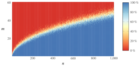
We report in Table 1 experimental results for different values of . We chose all the , for , to be independent random variables uniformly distributed on . Moreover, the diagonal coefficients were chosen to have a positive tropical sign (they belong to ). We took (the performance was similar for or ). Our experiments were obtained using a C program, distributed as an ancillary file attached to this arXiv manuscript for reproducibility purposes.333The ancillary file can be downloaded from http://arxiv.org/src/1603.06916/anc. This program was compiled under Linux with gcc -O3, and executed on a single core of an Intel(R) i7-4600U CPU at 2.10 GHz with 16 GB RAM. We report the average execution time over 10 samples for every value of . The number of iterations did not exceed 731 on this benchmark, and, for most , it was limited to a few units. Indeed, random instances exhibit experimentally a phase transition, as shown in Figure 5: for a given , the system is either feasible with overwhelming probability, or infeasible with overwhelming probability, unless lies in a tiny region of the parameter space. Value iteration quickly decides feasibility, except in regions close to the phase transition. This explains why the execution time does not increase monotonically with in our experiments (we included both easy and hard values of ).
| time | 0.000065 | 0.000049 | 0.000077 | 0.000279 | 0.026802 |
| time | 0.000025 | 0.000270 | 0.000366 | 0.000656 | 0.053944 |
| time | 0.000233 | 0.073544 | 0.015305 | 0.027762 | 0.148714 |
| time | 0.000487 | 1.852221 | 0.087536 | 19.919844 | 2.309174 |
7. Equivalent forms of stochastic mean payoff games problem
In this section we present the (algorithmically) equivalent forms of stochastic mean payoff games, as mentioned in Remark 8. In order to do that, we need to introduce the notions of simple stochastic games and stopping games.
We start by defining the class of stopping games. We say that a pair of states is a sink if, when or is reached, the game loops forever between these two states. More formally, we have . We say that the game is stopping if it has at least one sink and the probability that the game will reach a sink is equal one for every choice of policies and every initial state. Note that if a game is stopping, then only the payoffs in sinks are important to determine its solution. Indeed, if we denote the sinks by and the game is stopping, then the payoff of Player Max is given by
where is the probability that the game starting from reaches the sink if the players use the policies . This expression depends only on payoffs in sinks.
Now, we introduce the class of simple stochastic games. We say that the stochastic game is simple if its set of states can be divided into three classes: states controlled by Player Min, Player Max, and Nature. Players Min and Max have only deterministic choices and Nature chooses the next state by tossing a coin. (To be coherent with the previous definition of stochastic game, we assume that Player Min controls the states of Nature — but she has no other choice than to toss a coin.) Formally, we suppose that for every and every we have the implication . Moreover, a simple game has two sinks: one with payoff and the other with payoff . All other payoffs are equal to .
It may seem that solving simple games is indeed simpler that solving games in their full generality. Andersson and Miltersen [AM09] have shown that this is not the case. Let Smpg-comp denote the problem of finding the value and a pair of optimal policies in a stochastic mean payoff game.
Theorem 47 ([AM09]).
Smpg-comp is poly-time equivalent to the problem of finding the values of stopping simple stochastic games.
Note that this theorem was originally without the word “stopping”, but this is what the authors actually showed in the latter reference. As already mentioned in Remark 8, this result is valid for a much wider class of games than those considered in this work. Andersson and Miltersen defined stopping simple stochastic games in a slightly more general way — in their version, the players can make multiple moves in a row. Nevertheless, observe that we can always add dummy states to a stopping simple stochastic game (i.e., states in which player has only one action) and obtain an equivalent game that belongs to the class considered here. This shows that, from the algorithmic point of view, these classes are equivalent.
Moreover, observe that if the game is both simple and stopping, then we can change its payoffs in sinks — instead of payoffs equal to and , we can demand them to be equal to and . This does not change the optimal policies of the game and acts as an affine transformation on the value vector. Henceforth, we assume that payoffs in sinks of stopping simple stochastic games are equal to and . We now show that the computational problem of finding values of simple games can be reduced to the decision problem. By Smpg() we will denote the problem of deciding if a given state is winning in the stochastic mean payoff game.
Lemma 48.
Smpg() restricted to stopping simple stochastic games is poly-time equivalent to Smpg-comp.
Proof.
It is obvious that Smpg() can be reduced to Smpg-comp. We will show the opposite reduction. By Theorem 47, Smpg-comp is poly-time reducible to the problem of finding values of stopping simple stochastic games. Fix such a game and let denote its value.
First, we show an auxiliary reduction. Fix a rational number and an initial state . Suppose that we want to decide if . We will show that this is poly-time reducible (poly-time in the size of the game and the number of bits needed to encode ) to Smpg(). If , then the answer is “yes”. If , then we may modify the game as follows: we suppose that when the sink with payoff is reached, the game does not start to loop, but instead moves with probability to the sink with payoff and with probability to the (newly created) sink with payoff . Denote the value of the modified game by . We have . The modified game is stopping but not simple. Nevertheless, we may apply the construction of Zwick and Paterson [ZP96, remarks preceding Theorem 6.1] and obtain (in poly-time) a new game, which is stopping, simple, and has as the value at state . This gives the auxiliary reduction.
Finally, we want to show that Smpg() is poly-time reducible to Smpg. This requires an auxiliary construction which is presented in Figure 6. We take a stopping simple stochastic game , fix an initial state and suppose that the sinks of are indexed as (sink with payoff ) and (sink with payoff ). Now, we modify the game as follows: we add two states, (controlled by Player Min) and (controlled by Player Max). At , Player Min has only one possible action: to go to ; after this action Player Min pays to Player Max. Moreover, at Player Max also has only one action: to go to ; after this action Player Max receives from Player Min. Finally, we modify the sinks of as follows: at (resp. ) Player Max has only one possible action: to go to ; after this action he receives (resp. ) from Player Min. Denote the modified game by . By construction, it is quite intuitive that the value of does not depend on the initial state and that the state is winning in if and only if it is winning in . To prove this formally, we use Theorem 53. Henceforth, by we denote the -player game obtained from by fixing a pair of policies .
Corollary 49.
The state is winning in if and only if it is winning in . Moreover, the value of is independent of the initial state.
Proof.
First, observe that there exists a natural bijection between policies of and . Hence, we will use the same letters to denote policies in both games. Fix a pair of policies . Let (resp. ) denote the payoff of Player Max in (resp. in ). Since was stopping, the -player game obtained from by fixing the policies has only one recurrent class and belongs to this class. By Theorem 53 we see that is constant for all initial states. Since are arbitrary, this shows that the value of does not depend on the choice of initial state. Furthermore, Theorem 53 shows that , where is the expected time of first return to .
Now, suppose that the value of starting from is higher or equal than . Let denote the optimal policy of Player Max in . For any policy of Player Min we have and hence . Therefore, is a winning (but not necessarily optimal) policy for Player Max in starting from . Thus, the value of starting from is higher or equal than . The opposite implication is analogous. ∎
Corollary 50.
Smpg-comp is poly-time equivalent to Smpg restricted to games with payoffs in .
Proof.
Corollary 51.
Smpg restricted to games with payoffs in is poly-time equivalent to Smpg for general games.
Proof.
Smpg is trivially reducible to Smpg-comp. Therefore, the claim follows from Corollary 50. ∎
8. Concluding remarks
In this paper, we have shown that under a genericity condition on the valuations, solving feasibility semidefinite problems over the field of Puiseux series reduces to a well studied class of zero-sum stochastic games. This leads both to complexity bounds and to algorithms capable experimentally to solve large scale nonarchimedean instances. The interest is also to relate two different problems which both have unsettled complexities. This is the first exposition of this approach.
It would be interesting to relax the current genericity conditions. We believe that finer genericity conditions could involve both the valuations and leading coefficients of the series.
Another interesting question is to use the present approach to deal with the real case. We already showed in Section 5.3 that the nonarchimedean feasibility problem is equivalent to the archimedean one for large values of , with an exponential number of bits. We may ask however whether it is possible to use combinatorial methods to work for smaller values of .
Acknowledgments
We are grateful to the anonymous reviewers for their numerous remarks which helped to improve the presentation of the paper. An abridged version of the present work appeared initially in the ISSAC paper [AGS16a]. We also thank the referees of ISSAC for their detailed comments.
References
- [ACS14] D. Auger, P. Coucheney, and Y. Strozecki. Finding optimal strategies of almost acyclic simple stochastic games. In Proceedings of the 11th Annual Conference on Theory and Applications of Models of Computation (TAMC), volume 8402 of Lecture Notes in Comput. Sci., pages 67–85. Springer, 2014.
- [ACTDG13] M. Akian, J. Cochet-Terrasson, S. Detournay, and S. Gaubert. Solving multichain stochastic games with mean payoff by policy iteration. In 52nd IEEE Annual Conference on Decision and Control (CDC), pages 1834–1841. IEEE, 2013.
- [AGG09] M. Akian, S. Gaubert, and A. Guterman. Linear independence over tropical semirings and beyond. In Proceedings of the International Conference on Tropical and Idempotent Mathematics, volume 495 of Contemp. Math., pages 1–38. AMS, 2009.
- [AGG12] M. Akian, S. Gaubert, and A. Guterman. Tropical polyhedra are equivalent to mean payoff games. Int. J. Algebra Comput., 22(1):125001 (43 pages), 2012.
- [AGH15] M. Akian, S. Gaubert, and A. Hochart. Ergodicity conditions for zero-sum games. Discrete Contin. Dyn. Syst., 35(9):3901–3931, 2015.
- [AGS16a] X. Allamigeon, S. Gaubert, and M. Skomra. Solving generic nonarchimedean semidefinite programs using stochastic game algorithms. In Proceedings of the 41st International Symposium on Symbolic and Algebraic Computation (ISSAC), pages 31–38. ACM, 2016.
- [AGS16b] X. Allamigeon, S. Gaubert, and M. Skomra. Tropical spectrahedra. arXiv:1610.06746v2, 2016.
- [AM09] D. Andersson and P. B. Miltersen. The complexity of solving stochastic games on graphs. In Proceedings of the 20th International Symposium on Algorithms and Computation (ISAAC), volume 5878 of Lecture Notes in Comput. Sci., pages 112–121. Springer, 2009.
- [BB16] M. Baker and N. Bowler. Matroids over hyperfields. arXiv:1601.01204, 2016.
- [BPT13] G. Blekherman, P. A. Parrilo, and R. R. Thomas. Semidefinite Optimization and Convex Algebraic Geometry, volume 13 of MOS-SIAM Ser. Optim. SIAM, Philadelphia, PA, 2013.
- [But10] P. Butkovič. Max-linear Systems: Theory and Algorithms. Springer Monogr. Math. Springer, London, 2010.
- [CC11] A. Connes and C. Consani. The hyperring of adèle classes. J. Number Theory, 131(2):159–194, 2011.
- [Chu67] K. L. Chung. Markov Chains With Stationary Transition Probabilities, volume 104 of Grundlehren Math. Wiss. Springer, Heidelberg, 1967.
- [Con92] A. Condon. The complexity of stochastic games. Inform. and Comput., 96(2):203–224, 1992.
- [dKV16] E. de Klerk and F. Vallentin. On the Turing model complexity of interior point methods for semidefinite programming. SIAM J. Optim., 26(3):1944–1961, 2016.
- [FV07] J. Filar and K. Vrieze. Competitive Markov Decision Processes. Springer, New York, 2007.
- [GLS93] M. Grötschel, L. Lovász, and A. Schrijver. Geometric Algorithms and Combinatorial Optimization, volume 2 of Algorithms Combin. Springer, Berlin, 1993.
- [GM12] B. Gärtner and J. Matoušek. Approximation Algorithms and Semidefinite Programming. Springer, Heidelberg, 2012.
- [Hal07] N. Halman. Simple stochastic games, parity games, mean payoff games and discounted payoff games are all LP-type problems. Algorithmica, 49(1):37–50, 2007.
- [HNSED16] D. Henrion, S. Naldi, and M. Safey El Din. Exact algorithms for linear matrix inequalities. SIAM J. Optim., 26(4):2512–2539, 2016.
- [HR15] G. H. Hardy and M. Riesz. The general theory of Dirichlet’s series. Cambridge University Press, Cambridge, 1915.
- [HZ15] T. D. Hansen and U. Zwick. An improved version of the Random-Facet pivoting rule for the simplex algorithm. In Proceedings of the 47th Annual ACM Symposium on the Theory of Computing (STOC), pages 209–218. ACM, 2015.
- [KM03] S. Kwek and K. Mehlhorn. Optimal search for rationals. Inform. Process. Lett., 86(1):23–26, 2003.
- [Koh80] E. Kohlberg. Invariant half-lines of nonexpansive piecewise-linear transformations. Math. Oper. Res., 5(3):366–372, 1980.
- [LL69] T. M. Liggett and S. A. Lippman. Stochastic games with perfect information and time average payoff. SIAM Rev., 11(4):604–607, 1969.
- [MC11] D. Monniaux and P. Corbineau. On the generation of Positivstellensatz witnesses in degenerate cases. In Proceedings of the Second international conference on Interactive theorem proving (ITP), pages 249–264. ACM, 2011.
- [Meg89] N. Megiddo. On the complexity of linear programming. In T. F. Bewley, editor, Advances in economic theory, volume 12 of Econom. Soc. Monogr., pages 225–268. Cambridge University Press, Cambridge, 1989.
- [MS15] D. Maclagan and B. Sturmfels. Introduction to Tropical Geometry, volume 161 of Grad. Stud. Math. AMS, Providence, RI, 2015.
- [Nal18] S. Naldi. Solving rank-constrained semidefinite programs in exact arithmetic. J. Symbolic Comput., 85:206–223, 2018.
- [NRS10] J. Nie, K. Ranestad, and B. Sturmfels. The algebraic degree of semidefinite programming. Math. Program., 122(2):379–405, 2010.
- [Nus86] R. D. Nussbaum. Convexity and log convexity for the spectral radius. Linear Algebra Appl., 73:59–122, 1986.
- [Put05] M. L. Puterman. Markov Decision Processes: Discrete Stochastic Dynamic Programming. Wiley Ser. Probab. Stat. Wiley, Hoboken, NJ, 2005.
- [Ram97] M. V. Ramana. An exact duality theory for semidefinite programming and its complexity implications. Math. Program., 77(1):129–162, 1997.
- [Sch16] C. Scheiderer. Sums of squares of polynomials with rational coefficients. J. Eur. Math. Soc., 18(7):1495–1513, 2016.
- [Ste10] S. A. Steinberg. Lattice-ordered Rings and Modules. Springer, New York, 2010.
- [vdDS98] L. van den Dries and P. Speissegger. The real field with convergent generalized power series. Trans. Amer. Math. Soc., 350(11):4377–4421, 1998.
- [Vir10] O. Viro. Hyperfields for tropical geometry I. Hyperfields and dequantization. arXiv:1006.3034, 2010.
- [Yu15] J. Yu. Tropicalizing the positive semidefinite cone. Proc. Amer. Math. Soc., 143(5):1891–1895, 2015.
- [ZP96] U. Zwick and M. Paterson. The complexity of mean payoff games on graphs. Theoret. Comput. Sci., 158(1–2):343–359, 1996.
Appendix A Constructing spectrahedra from mean payoff games
Let be a stochastic mean payoff game, and let be the matrices as constructed in the paragraph following Theorem 23. From these matrices, we can define the set as in Definition 21. Denoting by the Shapley operator of , we still have:
Lemma 52.
For any we have .
Proof.
Let
denote the Shapley operator of . As in the proof of Lemma 22, we have the equivalence
We want to show that the last set of constraints describes . To do this, recall that an inequality of the form is equivalent to if , and to if . Therefore, for every we have the equivalence
| (14) | ||||
Moreover, note that if verifies (14), then we have the equality
| (15) |
Indeed, if we have for some , then by the construction we get and . In particular, , what gives a contradiction with (14). Furthermore, observe that for any we have the equality
| (16) |
Suppose that . Then verifies (14) for all . Hence, by (15) and (16), for any we have
| (17) | ||||
Thus . Conversely, if , then also verifies (14) for all , and the same argument as in (17) shows that . ∎
Appendix B Markov chains
Let us recall some facts about Markov chains with rewards. We only consider Markov chains on finite spaces. Suppose that we are given a Markov chain defined on a finite space . Recall that such a chain can be described by a transition matrix , where denotes the probability that chain moves from state to state in one step.
If , then we say that is a stationary distribution on the set if for all and . Furthermore, a set is called a recurrent class if it has the following two properties: (a) if is reached, then the chain will never leave it; (b) if is reached, then every state in will be visited infinitely many times (with probability one). Every Markov chain has at least one recurrent class, and every recurrent class has a unique stationary distribution. A state is called recurrent if it belongs to a recurrent class. Otherwise, it is called transient.
We now introduce Markov chains with payoffs. To this end, with every state we associate a payoff . This quantity is interpreted as follows: there is a controller of the chain, who receives a payoff as soon as the chain leaves the state . A (long-term) average payoff of the controller is defined as
where the expectation is taken over all trajectories starting from in the Markov chain. The next theorem characterizes the average payoff. Before that, let us introduce some additional notation.
For any state , let the random variable denote the time of first return to . By we denote the expected time of first return to ,
Furthermore, let be the expected payoff the controlled obtained before returning to , i.e.,
Theorem 53.
If is a fixed initial state, then the average payoff is well defined and characterized as follows:
-
(i)
Suppose that is a recurrent state belonging to the recurrent class . Let be the stationary distribution on . Then . Furthermore, we have
In particular, is constant for all states belonging to .
-
(ii)
If is transient and denote all the recurrent classes of the Markov chain, then , where, for all , denotes the probability that the chain starting from reaches the recurrent class , and is an arbitrary state of .
Remark 54.
We point out that given the transition matrix , the average payoff can be computed using the algorithm presented in [Put05, Appendix A.3 and A.4]. This algorithm can be implemented to run in strongly polynomial complexity using the strongly polynomial version of gaussian elimination (presented, for example, in [GLS93, Section 1.4]).
Theorem 53 is well known, and can be easily derived from the analysis of Markov chains presented in the textbook of Chung [Chu67, Part I, §6, §7, and §9]. We give the details for the sake of completeness. Let denote the probability that the Markov chain starting from will reach at least once, . By definition, the state is recurrent if , and it is transient otherwise. By we denote the expected number of visits in before returning to , i.e.,
The following theorem describes the ergodic behavior of any finite (or countable) Markov chain.
Theorem 55.
The Cesaro limit
is well defined (we will denote it by ). Moreover, the entries of are given as follows: if is a transient state, then for all . If is recurrent, then for all .
Proof.
See [Chu67, Part I, §6, Theorem 4 and its Corollary]. ∎
Remark 56.
Note that the theorem above does not state that if the state is recurrent. (We work under the convention that for all finite .) Nevertheless, if the chain is finite, then we have for all recurrent states , and this can be deduced as a corollary of the theorem above, as discussed below.
Observe that is a stochastic matrix (as a limit of stochastic matrices). Moreover, we have . This leads to the following corollary.
Corollary 57.
If is a recurrent class, then for all . Furthermore, defined as is the unique stationary distribution on . In particular, if is a recurrent state, then .
Proof.
Let first claim follows immediately from Theorem 55. We will prove that is a stationary distribution on . Let denote the square submatrix of formed by the rows and columns of with indices in . We define analogously. The first claim implies that has identical rows. Since is a recurrent class, we have for all . Hence, for all we have . Therefore . Hence, is stochastic. In other words, every row of is a probability distribution on and, since , this distribution is a stationary distribution on . Since is a recurrent class, stationary distribution on has only strictly positive values. Hence we have . The fact that the stationary distribution is unique follows from [Chu67, Part I, §7, Theorem 1]. ∎
The next theorem characterizes the relationship between entries of and the values .
Theorem 58.
If belong to the same recurrent class, then . Moreover, if are (not necessarily distinct) states belonging to the same recurrent class, then .
Proof.
Corollary 59.
If belong to the same recurrent class, then
Proof of Theorem 53.
Fix . Observe that for all we have
Therefore . In particular, is well defined.
Let us suppose that the initial state is recurrent and denote its recurrent class by . In this case, Corollary 57 and Theorem 55 imply that , where is the stationary distribution on . Moreover, Corollary 59 gives the identity
Now, suppose that the initial state is transient. Let denote the recurrent classes in our Markov chain. In this case, Theorem 55 gives the identity