Completely random measures for modeling
power laws in sparse graphs

Abstract

Network data appear in a number of applications, such as online social networks and biological networks, and there is growing interest in both developing models for networks as well as studying the properties of such data. Since individual network datasets continue to grow in size, it is necessary to develop models that accurately represent the real-life scaling properties of networks. One behavior of interest is having a power law in the degree distribution. However, other types of power laws that have been observed empirically and considered for applications such as clustering and feature allocation models have not been studied as frequently in models for graph data. In this paper, we enumerate desirable asymptotic behavior that may be of interest for modeling graph data, including sparsity and several types of power laws. We outline a general framework for graph generative models using completely random measures; by contrast to the pioneering work of Caron and Fox (2015), we consider instantiating more of the existing atoms of the random measure as the dataset size increases rather than adding new atoms to the measure. We see that these two models can be complementary; they respectively yield interpretations as (1) time passing among existing members of a network and (2) new individuals joining a network. We detail a particular instance of this framework and show simulated results that suggest this model exhibits some desirable asymptotic power-law behavior.

1 Introduction

In recent years, network data has increased in both ubiquity and size. As network data appear in a growing number of applications—such as online social networks, biological networks, and networks representing communication patterns—there is growing interest in developing models and inference for such data and studying its properties. Bayesian generative models for network data include, but are not limited to, the stochastic block model [10] and variants [13, 24], the infinite relational model [13], the latent feature relational model [16], the infinite latent attribute model [20], and the random function model [15].

Crucially, individual network data sets also continue to increase in size. Thus, it is not enough to develop models for networks, but in particular it is necessary to develop models that accurately represent the real-life scaling properties of networks. As particular networks increase in size, it has already become apparent that all of the models listed above share at least one undesirable scaling property. In particular, they all fit the assumptions of the Aldous–Hoover Theorem [2, 11], which implies that they all generate dense graphs with probability one [19]. Here, we say a graph is dense if the number of edges in the graph grows asymptotically as the square of the number of vertices in the graph. By contrast, we say a graph is sparse if the number of edges grows sub-quadratically as a function of the number of vertices in the graph.

This disconnect between desired asymptotic behavior and model specifications motivates the development of new models that achieve sparsity rather than always generating dense graphs. Some initial work in this direction has been pioneered by Caron and Fox [5]. But just as a wide variety of models with a wide variety of behaviors are available for other applications, it is desirable to populate a broader toolbox of appropriate models for network data.

It remains to cultivate a more complete understanding of what behaviors are desirable in network data. Dense graphs are generally considered undesirable. But graph dense-ness describes just one potential graph behavior. Scaling behavior has been much more extensively studied in other domains. Since power laws are widely observed in real data [17, 18, 6], these investigations into scaling have tended to focus on power law behaviors. For instance, Gnedin et al. [7] have thoroughly characterized a wide variety of power laws that may be exhibited in clustering models and have, moreover, shown that many of these power laws are equivalent. One behavior of interest is a power law in the number of clusters as the number of data points grows. This behavior is roughly analogous to considering a power law in the number of edges as the number of vertices grows. But Gnedin et al. [7] consider a much wider range of potential power laws. Likewise, Broderick et al. [3] have enumerated a range of power laws for feature allocations, a generalization of clustering where each data point may belong to any non-negative integer number of groups—now called features instead of clusters. While some authors have drawn connections between feature allocations and certain types of networks [4], an exhaustive enumeration of asymptotic network behaviors of interest in graph data—beyond the simple divide between dense and sparse graphs—is still missing.

Not only have previous authors studied power laws for clustering and feature allocations, but they have detailed particular, practical generative models for achieving these power laws—and these models typically lead to corresponding inference algorithms as well. For instance, the canonical power law model for clustering is the Pitman–Yor process [21, 8, 23], and the canonical power-law model for feature allocations is the three-parameter beta process [22, 3].

Below we outline a general framework for graph generative models in Section 2. We detail a particular instance of our framework that gives a (new) generative model for networks that may be applied in practice. We develop a list of asymptotic behaviors of interest in network models in Section 3. In Section 4, we show preliminary results that suggest this model exhibits some desirable asymptotic (power-law) behavior. And we suggest empirical, theoretical, and algorithmic developments for future research in Section 5.

2 Generative framework

We first consider a general framework for generating graphs. Then we consider a specific case using completely random measures. Lastly, we show how this can be used to create models in practice by consider a beta process as the underlying completely random measure.

2.1 Motivation

Let $(\Omega,\Sigma,\mathbf{P})$ be a probability space. A random measure $W$ on $(\Omega,\Sigma)$ is a random measure-valued element such that $W(A)$ is a random variable for any measurable set $A\in\Sigma$.

Now suppose $W$ is an atomic random measure with atoms $(\theta_{i})_{i=1,\ldots,M}$ and weights $(w_{i})_{i=1,\ldots,M}$, where for all $i$, we have $w_{i}\in(0,1)$, that is,

$$W=\sum_{i=1}^{M}w_{i}\delta_{\theta_{i}},$$

where $M$ may be random or infinite. In this case, we can use the weights to generate the adjacency matrix $G$ of a graph by independently drawing edges ($G_{ij}=1$) with probability $w_{i}w_{j}$. Given $W$, we can draw a multigraph, in which edges can have multiplicity, by drawing edges independently and identically $N$ times.

We imagine each $\theta_{i}$ as corresponding to a vertex. So $w_{i}w_{j}$ is the probability of an edge forming between the vertices corresponding to $\theta_{i}$ and $\theta_{j}$. Thus, if $M$ is infinite, we theoretically have a countably infinite vertex set. However, another perspective is that only vertices that participate in some edge count toward the total number of vertices; we call the vertices that are connected via any edge effective vertices. From this perspective, having an infinite latent vertex collection ($M=\infty$) is necessary to allow the number of effective vertices to grow without bound. Completely random measures provide an option for generating a countably infinite number of atoms in our random measure $W$.

A completely random measure $W$ on $(\Omega,\Sigma)$ is a random measure with the additional requirement such that for any finite, disjoint measurable sets $A_{1},\ldots,A_{n}\in\Sigma$, the random variables $W(A_{1}),\ldots,W(A_{n})$ are (pairwise) independent [14]. Completely random measures can be constructed from a Poisson point process with rate measure $\nu(d\theta,dw)$ in the following way: if we draw a sample $(\theta_{i},w_{i})_{i\in{{\mathbb{N}}}}$ from a Poisson point process, we construct $W$ as follows:

$$W=\sum_{i=1}^{\infty}w_{i}\delta_{\theta_{i}}.$$

All completely random measures can be obtained in this way (along with a deterministic component and a fixed atomic component) [14].

2.2 Generative model

Let $W$ be a draw from the Poisson point process component of a completely random measure, where we assume that $\nu(d\theta,dw)$ has support on $w\in(0,1)$. To sample a graph given $W$, we draw an edge connection $C_{n,i,j}\stackrel{{\scriptstyle\text{ind}}}{{\sim}}\text{Bernoulli}(w_{i}w_{j})$, for $n=1,\ldots,N$, resulting in $G_{N,i,j}=\sum_{n=1}^{N}C_{n,i,j}$ edges for each pair of vertices $(i,j)$. For simplicity, we assume there are no loops; however, it is straightforward to adapt the model to include loops. In this paper, we primarily consider the restriction of $G_{N}$ to a binary array $Z_{N}$, where $Z_{N,i,j}:=\min\{G_{N,i,j},1\}$.

This generative model can have the following interpretation: $N$ can be seen as “time passing,” where as $N$ grows, more links are being generated in the network, thus bringing in more edges as well as effective vertices (i.e., vertices that are connected to at least one other vertex).

2.3 Example using beta processes

The beta process is an example of a completely random measure with rate measure

$$\nu(d\theta,dw)=cw^{-1}(1-w)^{c-1}dw\,B_{0}(d\theta),$$

where $c>0$ is the concentration parameter and $B_{0}$ is the base measure. It is known that for feature allocation applications, the beta process does not give power law behavior in scaling of quantities such as the number of instantiated features.

However, an extension of the beta process, the three-parameter beta process, is known to give power laws in feature allocation [22, 3]. The three-parameter beta process has rate measure $\nu$, a $\sigma$-finite measure with density

$$\nu(d\theta,dw)=\frac{\Gamma(1+c)}{\Gamma(1-\alpha)\Gamma(c+\alpha)}w^{-1-\alpha}(1-w)^{c+\alpha-1}dw\,B_{0}(d\theta),$$ (1)

where $\alpha\in(0,1)$ and $c>-\alpha$. We denote a draw from the three-parameter beta process as $W\sim\text{BP}(\theta,\alpha,B_{0})$.

To obtain power law behavior in graphs, we are similarly interested in completely random measures which can produce such behavior.

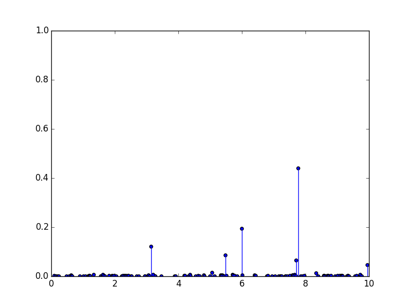
(a) Realization $W\sim\text{PP}(\nu)$

(b) A sample

Figure 1: A realization of $W$ when the underlying completely random measure is a three-parameter beta process, and the resulting binary graph $Z_{N}$ sampled given $W$. Here $N=100$ and the parameters of the beta process are $(\theta,\alpha,\gamma)$ = (1, 0.5, 5), where $\theta$ is the concentration parameter $\alpha$ is the discount parameter, and $\gamma$ is the Poisson rate parameter.

3 Power laws for graphs

It remains to be seen whether graph models produced under this framework exhibit desirable asymptotic and power law behaviors. For instance, we may be interested in graph behaviors similar to known power laws in partitions [7] and feature allocations [3]. In what follows, we define a number of power laws that may be of interest in graph modeling. In future work, we aim to characterize under what circumstances models fitting the framework from the previous section exhibit these power laws.

Graph quantities.

We first establish a few quantities of interest for which we want to define power laws. Note that all edge counts are considered with respect to the undirected graph given by the binary array $Z_{N}$, and for simplicity, we assume there are no loops; it is straightforward to adapt this section to graphs with loops.

We define the degree $D_{N,i}$ of a vertex $i$ to be

$$D_{N,i}:=\sum_{i\in{{\mathbb{N}}}}Z_{N,i,j}=\sum_{i\in{{\mathbb{N}}}}\mathbbm{1}\{G_{N,i,j}>0\},$$

i.e., the number of edges vertex $i$ is connected to.

A vertex $i$ has a triangle if, when $i$ is connected to a vertex $j$ and a vertex $k$, there is also an edge between $j$ and $k$. Let $T_{N,i}$ denote the number of triangles that $i$ participates in, i.e.,

$$T_{N,i}:=\sum_{j,k\in{{\mathbb{N}}}}\mathbbm{1}\{Z_{N,i,j}=1\}\mathbbm{1}\{Z_{N,i,k}=1\}\mathbbm{1}\{Z_{N,j,k}=1\}.$$

We define the effective number of vertices $\mathcal{V}_{N}$ to be the total number of vertices with nonzero degree:

$$\mathcal{V}_{N}:=\sum_{i\in{{\mathbb{N}}}}\mathbbm{1}\{D_{N,i}>0\}.$$

Note that in our definition, the number of vertices reflects the effective number of vertices in the network, rather than the size of the (infinite) adjacency matrix.

The total number of edges $\mathcal{E}_{N}$ is given by

$$\mathcal{E}_{N}:=\frac{1}{2}\sum_{i\in{{\mathbb{N}}}}D_{N,i}$$

We define the quantity

$$\mathcal{D}_{N,r}:=\sum_{i\in{{\mathbb{N}}}}\mathbbm{1}\{D_{N,i}=r\},$$

which gives the number of vertices with exactly degree $r$, and

$$\mathcal{T}_{N,r}:=\sum_{i\in{{\mathbb{N}}}}\mathbbm{1}\{T_{N,i}=r\},$$

which gives the number of vertices with exactly $r$ triangles.

We now characterize several types of power laws that may occur in graphs.

Type I power law: We first consider a power law in the asymptotic number of edges as a function of the asymptotic number of (effective) vertices.

$$\mathcal{E}_{N}\stackrel{{\scriptstyle\text{a.s.}}}{{\sim}}c\,\mathcal{V}_{N}^{a},\,N\rightarrow\infty,$$

for constants $c>0,a\in(1,2)$.

We might also consider power laws in the counts of vertices and triangles.

Type IIa power law: For instance, we might have a power law in the number of vertices of a certain degree.

$$\mathcal{D}_{N,r}\stackrel{{\scriptstyle\text{a.s.}}}{{\sim}}c\,\mathcal{V}_{N}^{a},\,N\rightarrow\infty$$

Type IIb power law: Similarly, we might have a power law in the number of vertices with a certain number of triangles

$$\mathcal{T}_{N,r}\stackrel{{\scriptstyle\text{a.s.}}}{{\sim}}c\,\mathcal{V}_{N}^{a},\,N\rightarrow\infty$$

Note that $c$ and $a$ need not be the same constants across these power laws.

These two types of power laws have behavior similar to Heaps’ law [9] and Zipf’s law [25] and have been studied extensively in a variety of real-world data. Some examples of graphs with this type of power law include the number of hyperlinks in relation to the number of users (and other variables) in an internet graph [17] and web caching strategies for the number of requests for webpages [1].

A fundamentally different type of power law reminiscent of the kind defined by Broderick et al. [3] for feature modeling is given by the distribution of a quantity on a vertex, rather than the asymptotic values of counts; the next type of power law gives a power law in the degree and triangle distribution.

Type IIIa power law: A power law for the degree distribution at a vertex $i$ is given by:

$$\Pr(D_{N,i}>M)\sim cM^{-a}.$$

Type IIIb power law: Similarly, we could consider the number of triangles at a vertex $i$:

$$\Pr(T_{N,i}>M)\sim cM^{-a}.$$

These types of power laws have been widely studied in a number of real-world graphs, such as degrees of proteins in a protein-interaction network of yeast, degrees of metabolites in the metabolic network of E. coli; see Mitzenmacher [17], Newman [18], Clauset et al. [6] for more details. Triangle distribution power laws have been observed in a number of real world social networks, such as LinkedIn and Twitter, and YahooWeb [12].

4 Simulations

In this section, we explore the behavior of graphs generated by this model via simulation. In particular, we are interested in seeing if the model can produce sparse graphs and whether it exhibits any of the power laws described in Section 3. We consider the case when the underlying completely random measure is the three-parameter beta process, i.e., we draw a realization $W\sim\text{BP}(\theta,\alpha,B_{0})$ according to the stick breaking representation given in Broderick, Jordan, and Pitman [3]:

$$W =\sum_{i=1}^{\infty}\sum_{j=1}^{C_{i}}V_{i,j}^{(i)}\prod_{l=1}^{i-1}(1-V_{i,j}^{(\ell)})\delta_{\psi_{i,j}}$$

$$C_{i} \stackrel{{\scriptstyle\text{iid}}}{{\sim}}\text{Pois}(\gamma)$$

$$V_{i,j}^{(\ell)} \stackrel{{\scriptstyle\text{ind}}}{{\sim}}\text{Beta}(1-\alpha,\theta+\ell\alpha)$$

$$\psi_{i,j} \stackrel{{\scriptstyle\text{iid}}}{{\sim}}\frac{1}{\gamma}B_{0}.$$

For the beta process we truncated the number of rounds to 5000, i.e., we drew 5000 Poisson random variables $C_{i}$. The parameters of the beta process were set as follows: $\gamma=3,\theta=1,\alpha=0.1$. The number of Bernoulli draws $N$ was varied at $N=50,\ldots,2000$ at increments of $10$.

In Figure 2, we show preliminary results from our simulations. Figure 2(a) shows the scaling of the number of vertices $V_{N}$ with the number of edges $E_{N}$. From this plot, we see that the model produces sparse behavior in graphs, as it is sub-quadratic in the scaling between the number of vertices and the number of edges. We examined the potential of having a type I power law by fitting a line to the higher number of vertices, which gave a slope of $1.2$. Thus, from our simulations, it appears that the scaling between the number of vertices and the number of edges follows a Type I power law.

In Figure 2(b), we show the scaling between the number of vertices $V_{N}$ and the number of vertices with degree 1 $D_{N,1}$. We checked the slope of the larger vertices, and found that these points had a slope of $1.1$. Thus, this simulation shows the appearance of a Type IIa power law relationship between the two quantities.

Lastly, we plot the degree distribution for a single graph when $N=100$ in Figure 2(c). For this plot, we checked the slope of the lower degrees and found a slope of $-1.6$; thus, it appears that this model produces a type IIIa power law in the degree distribution.

From our preliminary results, it seems promising that our framework generates graphs exhibiting several types of power laws. In future work, we will examine the behavior of other types of power laws, e.g., Type IIb and Type IIIb, and it remains to prove the asymptotic properties of our model.

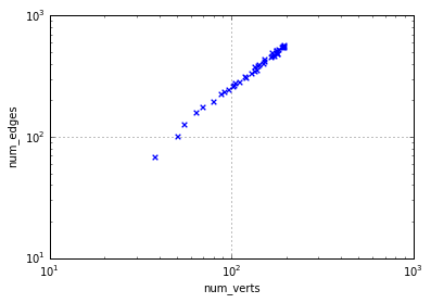
(a) Scaling of vertices $V_{N}$ vs edges $E_{N}$

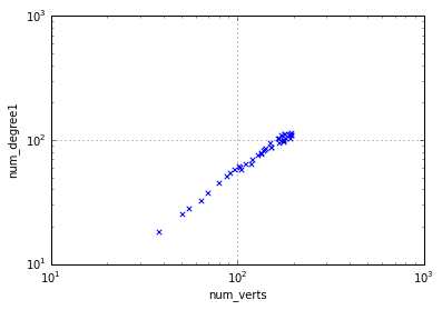
(b) Scaling of vertices with degree 1 $D_{N,1}$

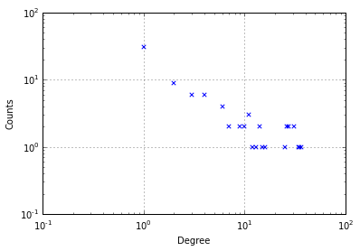
(c) Degree distribution, $N=100$

Figure 2: Simulated results of scalings of vertices and edges, the scaling of the vertices with number of degree 1 vertices, and the degree distribution of a single graph with $N=100$.

5 Future directions

We have described a framework for generating graphs using completely random measures and have characterized various types of power laws that may be desirable in a network model. In future work, we will study additional empirical power laws that can be obtained using a three-parameter beta process as well as other completely random measures. An important next step is to study the asymptotic scalings of quantities and distributions in graphs produced from this model. Here, we are interested in proving whether this model can produce certain power laws or whether it can be shown that the model does not produce those power laws. In addition to the types of power laws we examined empirically, in our theoretical analysis, we will investigate whether this model can also capture other kinds of power laws, such as the ones described in Section 3. Another direction is to fit the model using an efficient inference algorithm for this model on real-world networks. There are additional modeling extensions to explore, such as modeling block structure and sequential modeling (e.g., for triangles).

References

- Adamic and Huberman [2002] L. A. Adamic and B. A. Huberman. Zipf’s law and the internet. Glottometrics, 3(1):143–150, 2002.
- Aldous [1981] David J. Aldous. Representations for partially exchangeable arrays of random variables. J. Multivariate Anal., 11(4):581–598, 1981.
- Broderick et al. [2012] Tamara Broderick, Michael I. Jordan, and Jim Pitman. Beta processes, stick-breaking and power laws. Bayesian Anal., 7(2):439–475, 2012.
- Caron [2012] Francois Caron. Bayesian nonparametric models for bipartite graphs. In Adv. Neural Inform. Process. Syst. (NIPS) 25, pages 2060–2068, 2012.
- Caron and Fox [2014] Francois Caron and Emily B Fox. Bayesian nonparametric models of sparse and exchangeable random graphs. ArXiv e-print 1401.1137, 2014.
- Clauset et al. [2009] Aaron Clauset, Cosma Rohilla Shalizi, and Mark E. J. Newman. Power-law distributions in empirical data. SIAM Review, 51(4):661–703, 2009.
- Gnedin et al. [2007] Alexander Gnedin, Ben Hansen, and Jim Pitman. Notes on the occupancy problem with infinitely many boxes: general asymptotics and power laws. Probab. Surv., 4:146–171, 2007.
- Goldwater et al. [2005] Sharon Goldwater, Mark Johnson, and Thomas L Griffiths. Interpolating between types and tokens by estimating power-law generators. In Advances in neural information processing systems, pages 459–466, 2005.
- Heaps [1978] H. S. Heaps. Information retrieval: Computational and theoretical aspects. Academic Press, Inc., 1978.
- Holland et al. [1983] Paul W. Holland, Kathryn Blackmond Laskey, and Samuel Leinhardt. Stochastic blockmodels: first steps. Social Networks, 5(2):109–137, 1983.
- Hoover [1979] Douglas N. Hoover. Relations on probability spaces and arrays of random variables. Preprint, Institute for Advanced Study, Princeton, NJ, 1979.
- Kang et al. [2011] U. Kang, B. Meeder, and C. Faloutsos. Spectral analysis for billion-scale graphs: Discoveries and implementation. In Advances in Knowledge Discovery and Data Mining - 15th Pacific-Asia Conference, pages 13–25, 2011.
- Kemp et al. [2006] C. Kemp, J. B. Tenenbaum, T. L. Griffiths, T. Yamada, and N. Ueda. Learning systems of concepts with an infinite relational model. In Proc. 21st Nat. Conf. Artificial Intelligence (AAAI-06), 2006.
- Kingman [1993] J. F. C. Kingman. Poisson processes, volume 3 of Oxford Studies in Probability. The Clarendon Press, Oxford University Press, New York, 1993. Oxford Science Publications.
- Lloyd et al. [2012] James Robert Lloyd, Peter Orbanz, Zoubin Ghahramani, and Daniel M. Roy. Random function priors for exchangeable arrays with applications to graphs and relational data. In Adv. Neural Inform. Process. Syst. (NIPS) 25, 2012.
- Miller et al. [2009] Kurt T. Miller, Thomas L. Griffiths, and Michael I. Jordan. Nonparametric latent feature models for link prediction. In Adv. Neural Inform. Process. Syst. (NIPS) 22, pages 1276–1284, 2009.
- Mitzenmacher [2003] Michael Mitzenmacher. A brief history of generative models for power law and lognormal distributions. Internet Mathematics, 1(2):226–251, 2003.
- Newman [2005] Mark EJ Newman. Power laws, pareto distributions and zipf’s law. Contemporary physics, 46(5):323–351, 2005.
- Orbanz and Roy [2015] Peter Orbanz and Daniel M. Roy. Bayesian models of graphs, arrays and other exchangeable random structures. IEEE Trans. Pattern Anal. Mach. Intell., 37(2):437–461, Feb 2015.
- Palla et al. [2012] Konstantina Palla, David A. Knowles, and Zoubin Ghahramani. An infinite latent attribute model for network data. In Proc. 29th Int. Conf. Mach. Learn. (ICML), 2012.
- Pitman and Yor [1997] Jim Pitman and Marc Yor. The two-parameter poisson-dirichlet distribution derived from a stable subordinator. The Annals of Probability, pages 855–900, 1997.
- Teh and Gorur [2009] Yee W Teh and Dilan Gorur. Indian buffet processes with power-law behavior. In Advances in neural information processing systems, pages 1838–1846, 2009.
- Teh [2006] Yee Whye Teh. A hierarchical bayesian language model based on pitman-yor processes. In Proceedings of the 21st International Conference on Computational Linguistics, pages 985–992. Association for Computational Linguistics, 2006.
- Xu et al. [2007] Zhao Xu, Volker Tresp, Shipeng Yu, Kai Yu, and Hans-Peter Kriegel. Fast inference in infinite hidden relational models. In Proc. of Mining and Learning with Graphs (MLG 2007), 2007.
- Zipf [1949] G. K. Zipf. Human behavior and the principle of least effort. Addison-Wesley Press, 1949.