Tukey’s transformational ladder for portfolio management

Abstract

Over the past half-century, the empirical finance community has produced vast literature on the advantages of the equally weighted S&P 500 portfolio as well as the often overlooked disadvantages of the market capitalization weighted Standard and Poor’s (S&P 500) portfolio (see Bloomfield et al., (1977), DeMiguel et al., (2009), Jacobs et al., (2014), Treynor, (2005)). However, portfolio allocation based on Tukey’s transformational ladde have, rather surprisingly, remained absent from the literature. In this work, we consider the S&P 500 portfolio over the 1958-2015 time horizon weighted by Tukey’s transformational ladder (Tukey, (1977)): $1/x^{2},\,\,1/x,\,\,1/\sqrt{x},\,\,\text{log}(x),\,\,\sqrt{x},\,\,x,\,\,\text{and}\,\,x^{2}$, where $x$ is defined as the market capitalization weighted S&P 500 portfolio. Accounting for dividends and transaction fees, we find that the 1/$x^{2}$ weighting strategy produces cumulative returns that significantly dominates all other portfolios, achieving a compound annual growth rate of 18% over the 1958-2015 horizon. Our story is furthered by a startling phenomenon: both the cumulative and annual returns of the $1/x^{2}$ weighting strategy are superior to those of the $1/x$ weighting strategy, which are in turn superior to those of the 1/$\sqrt{x}$ weighted portfolio, and so forth, ending with the $x^{2}$ transformation, whose cumulative returns are the lowest of the seven transformations of Tukey’s transformational ladder. The order of cumulative returns precisely follows that of Tukey’s transformational ladder. To the best of our knowledge, we are the first to discover this phenomenon.

1 Introduction

For over half a century, the empirical finance community has extensively documented the advantages of the equally weighted Standard and Poor’s (S&P 500) portfolio as well as the often overlooked disadvantages of the market capitalization weighted S&P 500 portfolio (see Bloomfield et al., (1977), DeMiguel et al., (2009), Jacobs et al., (2014), Treynor, (2005)). In these works, novel statistical methodology has been created with the express purpose of analyzing alternative portfolio allocations. However, portfolio allocation based on the one of the most fundamental of statistical theories for data analysis, that of the seven transformations of John Tukey’s transformational ladder (Tukey, (1962), Tukey, (1977)), has, to the best of our knowledge, been overlooked by this large and impressive literature.
The motivation of the present paper is to infuse John Tukey’s transformational ladder into the empirical finance literature. We consider the S&P 500 portfolio from 1958-2015, and weight it by the entries of John Tukey’s transformational ladder (Tukey, (1977)): $1/x^{2},\,\,1/x,\,\,1/\sqrt{x},\,\,\text{log}(x),\,\,\sqrt{x},\,\,x,\,\,x^{2}$ (here, $x$ is the market capitalization weighted portfolio, which we henceforth abbreviate as “MKC”). Consider a market capitalization portfolio named “$x$” with two equities, equity I and equity II. Let equity I account for 40% of the total market capitalization of the portfolio and equity II account for 60% of the total market capitalization of the portfolio. The first of John Tukey’s transformations, the $1/x^{2}$ transformation, would assign weight

$$\frac{1/.4^{2}}{1/.4^{2}+1/.6^{2}},$$

(approximately .69) to equity I and a weight of approximately .31 to equity II. This logic for re-weighting a portfolio with two stocks is then naturally extended to re-weighting a portfolio with 500 stocks. The data obtained from The Center for Research in Security Prices (CRSP) also includes data on dividends for each stock, which we include throughout our analysis. We rebalance the portfolio monthly throughout the manuscript. We further assume transaction administrative fees of $1 (in 2015 dollars) per trade and, additionally, a long-run average bid-ask spread of .1% of the closing value of the stock. For example, if our portfolio buys (or sells) 50 shares of a given stock closing at $100, transaction fees of $1+ 50*(.1/2)= $3.5 are incurred.
This work presents two main findings. The first is that the 1/$x^{2}$ weighting strategy produces cumulative returns that significantly dominate all other portfolios, achieving a compound annual growth rate of 18% from 1958-2015. The second is that the $1/x^{2}$ portfolio’s compound annual growth rate is superior to the $1/x$ portfolio, which is in turn superior to 1/$\sqrt{x}$ portfolio, and so forth, ending with the $x^{2}$ transformation, whose cumulative returns are the lowest of the seven transformations of John Tukey’s transformational ladder. That is, the order of cumulative returns precisely follows that of Tukey’s transformational ladder.
Without further delay, we present our key findings. In Table 1 we display the compound annual growth rate (in %) of the equally weighted S&P 500 portfolio (EQU) and the seven Tukey transformations of the S&P 500, calculated from 1958-2015.

$1/x^{2}$	$1/x$	$1/\sqrt{x}$	$\text{log}(x)$	EQU	$\sqrt{x}$	MKC	$x^{2}$
18.00%	17.53%	15.23%	13.80%	13.32%	11.73%	10.43%	8.69%

Table 1: Compound annual growth rates (in %) of the EQU and the seven Tukey transformational ladder portfolios, calculated from 1958-2015.

Cumulative returns alone are insufficient for analyzing investment performance. To this end, we present annual returns for the eight portfolios under consideration. The mean annual returns, presented in Table 2 below, are calculated by taking an arithmetic mean of the 58 annual returns (1958-2015) for each portfolio.

$1/x^{2}$	$1/x$	$1/\sqrt{x}$	$\text{log}(x)$	EQU	$\sqrt{x}$	MKC	$x^{2}$
23.92%	20.35%	17.40%	15.62%	15.03%	13.18%	11.81%	10.25%

Table 2: The mean annual returns (in %) of the EQU and the seven Tukey transformational ladder portfolios, calculated by taking an arithmetic mean of the 58 annual returns (1958-2015) for each portfolio.

The associated sample standard deviations are as follows

$1/x^{2}$	$1/x$	$1/\sqrt{x}$	$\text{log}(x)$	EQU	$\sqrt{x}$	MKC	$x^{2}$
39.54%	26.44%	22.29%	20.01%	19.30%	17.52%	16.98%	18.05%

Table 3: Sample standard deviations of annual returns (in %) of the EQU and the seven Tukey transformational ladder portfolios, calculated by taking an the sample standard deviation of the 58 annual returns (1958-2015) for each portfolio.

The Sharpe ratios, calculated using a risk free rate of 1.75%, are

$1/x^{2}$	$1/x$	$1/\sqrt{x}$	$\text{log}(x)$	EQU	$\sqrt{x}$	MKC	$x^{2}$
56.07%	70.35%	70.21%	69.31%	68.81%	65.24%	59.25%	47.09%

Table 4: Sharpe ratios of the eight portfolios under consideration.

Table 1 shows that the compound annual growth rate of the $1/x^{2}$ portfolio, at 18.00%, beats the market capitalization weighted portfolio’s compound annual growth rate of 10.43% by a factor of 1.73. Table 2 displays that the arithmetic mean annual return of the $1/x^{2}$ weighted portfolio, at 23.92%, beats the market capitalization weighted portfolio’s arithmetic mean return of 11.81% by a factor of 2.03.
In his foreword to Bogle, (2000) (an articulate defense of the S&P 500 Index Fund), Professor Paul Samuelson writes that “Bogle’s reasoned precepts can enable a few million of us savers to become in twenty years the envy of our suburban neighbors–while at the same time we have slept well in these eventful times.” To use a strategy which is beaten by many others might not necessarily be a good thing. And yet, the S&P 500 market cap weighted portfolio is probably used more than any other. Indeed, the tables above show there are superior alternatives, and the equally weighted portfolio is one of the many available.
The remainder of this paper is organized as follows. Section 2 surveys related literature, with a specific emphasis on on the “small-firm effect” phenomenon. Section 3 provides an overview of the dataset and of the calculations employed. Section 4 offers an analysis of cumulative returns of the portfolios. Section 5 supplements Section 4 and Section 6 offers bootstrap simulations. Section 7 offers an analysis of annual returns of the portfolios, Section 8 calculates VaR and cVaR, and Section 9 offers concluding remarks. Appendices A, B, C, and D supplement the main manuscript.

2 Related Literature

The literature on the role of Tukey transforms in modern data analysis is vast (see Wojciechowski and Thompson, (2006), Thompson, (2011), Baggett and Thompson, (2007), and Tukey, (1962) for a few of the many resources). Remarkably, and to the best of our knowledge, there has been no existing literature on the use of Tukey transforms for the purposes of portfolio management. However, the “small-firm effect,” which refers to the superior performance of small-cap stocks relative to large-cap stocks, may easily be confused with the Tukey transformational ladder.
We briefly review some of the seminal empirical findings in the small-firm effect literature. The small-firm effect was first introduced into the literature by Banz, (1981), who empirically showed that during 1936-1975, the bottom quintile of stocks listed on the New York Stock Exchange (NYSE) achieved a .40% excess risk-adjusted return over all remaining stocks. The field was greatly furthered by Fama and French, (1992), who took a sample of stocks from NYSE, Amex, and Nasdaq over the period 1963-1990 and showed that the smallest 10% of firms in their database outperformed the largest 10% by .63% per month. However, empirical studies conducted since Fama and French, (1992) have largely concluded that the size effect died out sometime in the early 1980s. The seminal work of Horowitz et al., (2000) shows no evidence of size effect over the 1979-1995 time horizon and the work of Hirshleifer, (2001) argues that the size effect disappeared in 1983. We refer the reader to van Dijk, (2011) for a more complete accounting of this literature.
We wish to emphasize that our empirical results (presented in Section 4 and thereafter) neither contradict nor support the small-firm effect hypothesis, and therefore that results concerning Tukey’s transformational ladder for portfolio management must be viewed as their own distinct phenomena. At the present time, we do not have sufficient empirical evidence that the $1/x^{2}$ portfolio strategy does not ride on the size effect, and this matter will be investigated in future research.

3 Data and Index Methodology

Our data is the S&P 500 index from January 1958 to December 2015. The dataset was acquired from the Center for Research in Security Prices (CRSP). CRSP provides a reliable list of S&P 500 index constituents, their respective daily stock prices, shares outstanding, dividends, and any “key” events, such as stock splits and acquisitions. The dataset is updated accordingly when a company joins or leaves the S&P 500 constituent list. Further, the index returns are calculated for each portfolio according to the “index return formula” as documented by CRSP. CRSP computes the return on an index ($R_{t}$) as the weighted average of the returns for the individual securities in the index according to the following equation

$$R_{t}=\dfrac{\sum_{i}\omega_{i,t}\times r_{i,t}}{\sum_{i}\omega_{i,t}},\vspace{-0.25cm}$$ (1)

where $R_{t}$ is the index return, $\omega_{i,t}$ is the weight of security $i$ at time $t$, and $r_{i,t}$ is the return of security $i$ at time $t$.

3.1 Calculations

Throughout all calculations, we begin with an investment of $100,000 in 1958 dollars. According to the Consumer Price Index (CPI) from Federal Reserve Bank of St. Louis, this is equivalent to approximately $827,010.5 in 2015 dollars. Throughout all calculations, the transaction fees, which were documented in the second paragraph of Section 1, are discounted according to the CPI (for example, an administrative transaction fee of $1 in 2015 is equivalent to 12.1 cents in 1958). All portfolios, with the exception of those in Appendix B, are rebalanced monthly and the transaction fees are subtracted from the portfolio total at market close on the first trading day of every month. Dividends are included in all calculations.

3.2 Transaction fees

Below we provide a table of transaction fees incurred by each of the eight portfolios under consideration over the 1958-2015 horizon. All numbers are discounted according to the CPI. The total transaction fees are much lower for the MKC and EQU portfolios than the $1/x^{2}$ and $1/x$ portfolios, as these require the most frequent rebalancing.

	$1/x^{2}$		$1/x$		$1/\sqrt{x}$		$\log\left(x\right)$		EQU		$\sqrt{x}$		MKC		$x^{2}$
Administration	0.	171 mil	0.	171 mil	0.	171 mil	0.	171 mil	0.	171 mil	0.	171 mil	0.	171 mil	0.171 mil
Bid-ask Spread	10.	967 mil	4.	093 mil	0.	694 mil	0.	126 mil	0.	035 mil	0.	118 mil	0.	117 mil	0.098 mil
Total	11.	138 mil	4.	264 mil	0.	865 mil	0.	297 mil	0.	206 mil	0.	289 mil	0.	288 mil	0.269 mil

Table 5: Administration fee ($1 per trade) and bid-ask spread (0.1% of the closing price per stock) for each of the eight portfolios under consideration from 1958-2015. All portfolios are rebalanced monthly.

4 Cumulative returns from 1958 to 2015

We present our first main finding below in Figure 1. Figure 1 displays the cumulative returns calculated from 1958 to 2015 of the equally weighted S&P 500 portfolio (EQU) and the seven portfolios given by the Tukey transformations ($1/x^{2},\,\,1/x,\,\,1/\sqrt{x},\,\,\text{log}(x),\,\,\sqrt{x},\,\,x,\,\,x^{2}$), where $x$ is the market capitalization weighted portfolio. The calculation assumes that $100,000 (in 1958 dollars) is invested in each of portfolio on 1/2/58 and is left to grow until 12/31/15. All dividends and transaction fees are taken into account, here and in every figure and table produced in this work.

Figure 1: Cumulative $\text{log}_{10}$ returns (from 1958-2015) for the EQU portfolio and the seven Tukey transformational ladder portfolios. The calculation assumes that $100,000 is invested on 1/2/58 and is left to grow until 12/31/15.

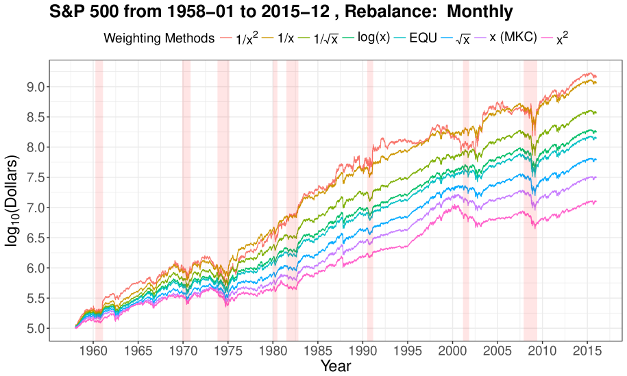
Figure 1 shows significant changes in portfolio returns over the 1958-2015 time horizon. Across all eight portfolios, the following macroeconomic events are well pronounced: the bear market from November 1968 to May 1970 (high inflation and the Vietnam war), the January 1973-October 1974 bear market (OPEC embargo), the 1982-1987 bull market, the “Black Monday” crash of October 1987, the 1988-2000 bull market, the dot-com bubble burst from March 2000 to October 2002, the most recent financial crisis of October 2007 to March 2009, and the most recent bull market which began in March 2009.
The cumulative returns on 12/31/15 displayed in Figure 1 are reproduced in Table 6 below.

$1/x^{2}$	$1/x$	$1/\sqrt{x}$	$\log\left(x\right)$	EQU	$\sqrt{x}$	$x$	$x^{2}$
$ 1.477 bil	$ 1.169 bil	$ 372.539 mil	$ 180.263 mil	$ 141.373 mil	$ 62.217 mil	$ 31.516 mil	$ 12.544 mil

Table 6: Cumulative values on 12/31/15 for EQU and all seven Tukey transformational ladder portfolios.

4.1 Discussion of Table 6

Our first main finding is exhibited by Table 6, which shows that investing $100,000 in January 1958 in the $1/x^{2}$ portfolio yields a cumulative value of $1.477 billion in December 2015. As such, the $1/x^{2}$ portfolio’s value on 12/31/15 remarkably dominates all other seven portfolios by a substantial margin; in particular, it exceeds the market capitalization’s cumulative value of $31.516 million by a factor of 46.865! The dominance of the $1/x^{2}$ weighted portfolio cumulative return will be explored on theoretical grounds in a future paper and as such is beyond the scope of the present work. For the purposes of this paper, we favor an intuitive explanation. The $1/x^{2}$ portfolio assigns the large majority of its weight to the lowest cap stocks of the S&P 500, very little weight to the larger cap stocks of the S&P 500, and negligible weight to the largest cap stocks of the S&P 500. Consequently, the portfolio reaps the benefits from the “smaller cap stocks” of the S&P 500, the latter of which are more volatile and may present more opportunity for growth.
Our second main finding from Table 6 is that the cumulative values of the portfolios follow the precise order of Tukey’s transformational ladder. Namely, the cumulative value of the $1/x^{2}$ portfolio is largest, followed by the $1/x$, $1/\sqrt{x}$, $\text{log}(x)$, $\sqrt{x}$, and $x$ (MKC) portfolios, and ending with the $x^{2}$ portfolio. To the best of our knowledge, we are the first to discover this phenomenon.

Remark 1

The rabbis of the Babylonian Talmud are often credited to be the first to give explicit advice on wealth allocation. In the fourth century, Rabbi Isaac Bar Aha, wrote that “one should always divide his wealth into three parts: a third in land, a third in merchandise, and a third ready to hand.” Unlike Rabbi Isaac Bar Aha, perhaps the late John Tukey may have unknowingly offered suggestions for wealth management.

5 The Tukey transformational ladder for alternate time horizons

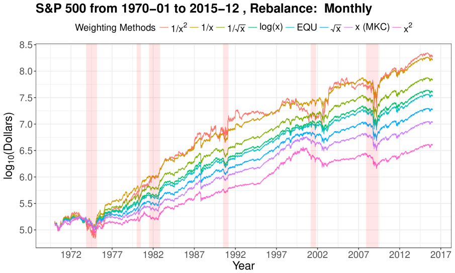
Figure 1 in Section 4 shows that the portfolio returns precisely follow the Tukey transformational ladder over the 1958-2015 time horizon. A natural line of inquiry is to determine whether the portfolio returns precisely follow the Tukey transformational ladder for other time horizons. We thus proceed to calculate the cumulative returns of the for the EQU and the seven Tukey transformations for four additional time periods: 1970-2015, 1980-2015, 1990-2015, and 2000-2015. The portfolio returns precisely follow the order of the Tukey transformational ladder over these additional four time periods.
We first consider the time horizon 1970-2015. We invest $132,168 on 1/2/70 (the equivalent of $100,000 in 1958 dollars) and let the portfolios grow until 12/31/15. The following cumulative portfolio values are presented in Figure 2 below.

Figure 2: Cumulative $\text{log}_{10}$ returns (from 1970-2015) for the EQU portfolio and the seven Tukey transformational ladder portfolios. The calculation assumes that $132,168 is invested on 1/2/70 and is left to grow until 12/31/15.

The cumulative returns displayed in Figure 2 are reproduced in Table 7 below.

$1/x^{2}$	$1/x$	$\sqrt{x}$	$\log\left(x\right)$	EQU	$\sqrt{x}$	$x$	$x^{2}$
$192.505 mil	$166.178 mil	$69.009 mil	$40.900 mil	$34.410 mil	$18.964 mil	$10.904 mil	$4.028 mil

Table 7: The cumulative returns for the EQU portfolio and the Tukey transformational ladder portfolios. The caclulation assumes that $132,168 is invested on 1/2/70 and is left to grow until 12/31/15.

The graphs and tables for the 1980-2015, 1990-2015, and 2000-2015 time horizons appear in Appendix D.

6 Bootstrap

We bootstrap each portfolio to obtain confidence intervals for each portfolio’s cumulative returns. Section 6.1 shows that the mean returns of the bootstrap distributions for random $N$ precisely follow the “modified” Tukey transformational ladder in the following sense: if one omits the $1/x^{2}$ portfolio from consideration, the bootstrapped means precisely follow the remainder of the Tukey transformational ladder (the $1/x$ transformation has the highest bootstrapped sample mean, followed by $1/\sqrt{x}$, $\text{log}(x)$, $\sqrt{x},x$, and culminating with $x^{2}$).

6.1 Bootstrap for Random $N$

We conduct a simple bootstrap as illustrated below in Algorithm 1. First, we uniformly choose the number of stocks $N$ from the sample space $\Omega=\left\{100,101,\ldots,500\right\}$. Second, we sample $N$ stocks with replacement from all listed stocks in S&P 500 from 1/2/58 to 12/31/15. We proceed to calculate the subsequent daily return using CRSP’s return on index formula

$$R_{t}=\dfrac{\sum_{i}\omega_{i,t}\times r_{i,t}}{\sum_{i}\omega_{i,t}},$$

where $R_{t}$ is the portfolio return on day $t$, $\omega_{i,t}$ is the weight of security $i$ on day $t$, and $r_{i,t}$ is the return of the security $i$ on day $t$. The variable $\omega_{i,t}$ is computed using a Tukey transformation of the market capitalization rate on day $t-1$. We then compute the cumulative returns using these daily returns and repeat the above process 20,000 times. The resulting bootstrap plots are presented in Figure 3, and the units are in million USD. The key idea is that the mean returns of the bootstrap distributions precisely follow the “modified” Tukey transformational ladder in the following sense: if one omits the $1/x^{2}$ portfolio from consideration, the bootstrapped means precisely follow the remainder of the Tukey transformational ladder (the $1/x$ transformation has the highest bootstrapped sample mean, followed by $1/\sqrt{x}$, $\text{log}(x)$, $\sqrt{x},x$, and finally culminating with $x^{2}$).

Figure 3: The bootstrap distribution produced using Algorithm 1. The estimated mean $\bar{x}$, standard deviation $\hat{\sigma}$, and 95% confidence intervals are displayed. All numbers are in million USD.

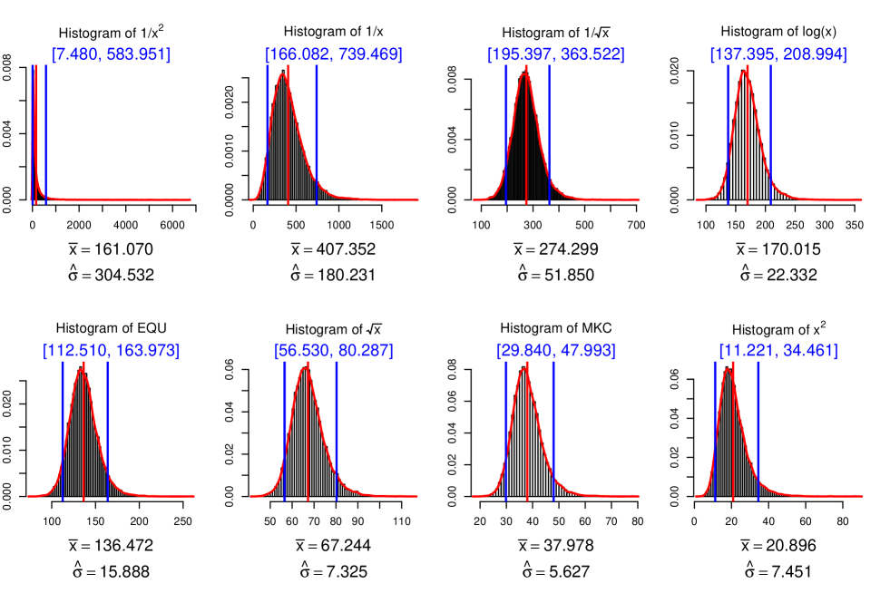
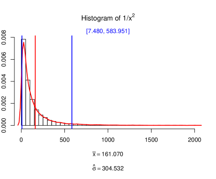
Higher resolution plots of the $1/x^{2}$ and $1/x$ bootstrap distributions are found below.

(a) $1/x^{2}$

(b) $1/x$

Figure 4: $1/x^{2}$ and $1/x$ bootstrap distributions.

  for $itr$ in $1,\cdots,10000$ do

     Sample $N$ from $\Omega=\left\{100,101,\cdots,500\right\}$.

     Sample $N$ stocks from the S&P 500 list randomly with replacement.

     for $t$ from 1958/01/03 to 2015/12/31 do

        if $k$ stocks are deleted from our selected portfolio on day $t$. then

           Randomly select the other $k$ remaining stocks in S&P 500 on day $t$ with replacement.

        end if

        Compute daily return $R_{t}$ for day $t$

$$R_{t}=\dfrac{\sum_{i}\omega_{i,t}\times r_{i,t}}{\sum_{i}\omega_{i,t}}$$

     end for

     Compute the cumulative return for iteration $itr$.

$$CR_{itr}=10^{5}\times\prod_{t=1}\left(1+R_{t}\right)$$

  end for

Algorithm 1 Bootstrap Sampling

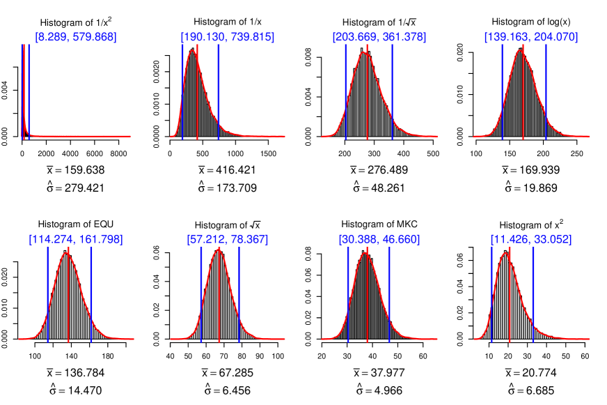
6.2 Bootstrap for Fixed $N$

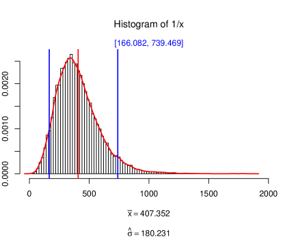
We now modify Algorithm 1 to conduct a bootstrap for fixed $N$. Below we produce the bootstrapped simulations for $N=10$ for the EQU portfolio and the seven portfolios of the Tukey transformational ladder for the 1/2/58-12/31/15 horizon. The following sample statistics are reported: the 1st percentile, the 5th percentile, the median, the mean, the 95th percentile, and the 99th percentile. The blue lines in each plot denote the 5th and 95th percentiles of the bootstrapped distribution.

Figure 5: The bootstrap distributions for $N=10$.

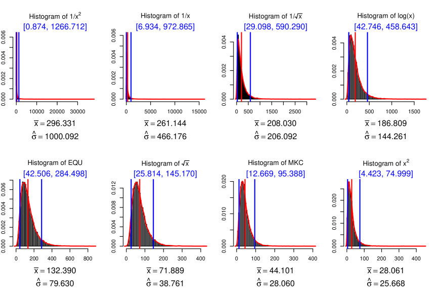
	mean	median	sd	q5th	q95th	q1th	q99th
$1/x^{2}$	296.331	50.890	1000.092	0.874	1266.712	0.135	3970.265
$1/x$	261.144	113.067	466.176	6.934	972.865	1.905	2158.401
$1/\sqrt{x}$	208.030	147.852	206.092	29.098	590.290	13.791	993.413
$\log\left(x\right)$	186.809	149.495	144.261	42.746	458.643	24.520	716.204
EQU	132.390	114.843	79.630	42.506	284.498	27.477	403.269
$\sqrt{x}$	71.889	63.964	38.761	25.814	145.170	16.674	200.863
$x$	44.101	37.897	28.060	12.669	95.388	7.260	141.100
$x^{2}$	28.061	21.734	25.668	4.423	74.999	1.997	122.697

Table 8: Sample statistics for the cumulative return on 12/31/15 for $N=10$, calculated from 20,000 simulations. All numbers are in million USD.

In the above results for $N=10$, the mean of the $1/x^{2}$ portfolio is highest, and the bootstrapped sample means precisely follow the order of the Tukey transformational ladder. The same holds true for the bootstrapped sample means for $N=20$ (see Appendix C). However, for $N=50$ and higher (see Appendix C), the $1/x$ bootstraped portfolio posts the highest sample mean. For these higher values of $N$, the bootstrapped means follow the “modified” Tukey transformational ladder. For $N=200,300,400,500$, the sample mean for the $1/x^{2}$ bootstrapped distribution falls above EQU, but below that of $\text{log}(x)$. We conclude that the $1/x^{2}$ transformation is not robust for fixed $N$ for large values of $N$.

7 Annual rates of return

Below we display the key findings from Tables 15 and 16 in Appendix A. Table 9 gives the mean annual returns (in %) of the EQU and the seven Tukey transformational ladder portfolios, calculated by taking an arithmetic mean of the 58 annual returns (1958-2015) for each portfolio.

$1/x^{2}$	$1/x$	$1/\sqrt{x}$	$\text{log}(x)$	EQU	$\sqrt{x}$	MKC	$x^{2}$
23.92%	20.35%	17.40%	15.62%	15.03%	13.18%	11.81%	10.25%

Table 9: The mean annual returns (in %) of the EQU and the seven Tukey transformational ladder portfolios, calculated by taking an arithmetic mean of the 58 annual returns (1958-2015) for each portfolio.

The associated sample standard deviations are as follows:

$1/x^{2}$	$1/x$	$1/\sqrt{x}$	$\text{log}(x)$	EQU	$\sqrt{x}$	MKC	$x^{2}$
39.54%	26.44%	22.29%	20.01%	19.30%	17.52%	16.98%	18.05%

Table 10: Sample standard deviations of annual returns (in %) of the EQU and the seven Tukey transformational ladder portfolios, calculated by taking an the sample standard deviation of the 58 annual returns (1958-2015) for each portfolio.

The associated Sharpe ratios, used a risk free rate of 1.75%, are:

$1/x^{2}$	$1/x$	$1/\sqrt{x}$	$\text{log}(x)$	EQU	$\sqrt{x}$	MKC	$x^{2}$
56.07%	70.35%	70.21%	69.31%	68.81%	65.24%	59.25%	47.09%

Table 11: Sharpe ratios of the eight portfolios under consideration.

The cumulative returns of the $1/x^{2}$ portfolio, as presented in Table 6, in addition to the average annual returns presented above in Table 11, indeed make it a tempting strategy for investment professionals and hedge funds. However, due to both its large standard deviation (see Table 10) and extremely high values of VaR and cVaR (see Section 8), the $1/x^{2}$ portfolio presents enormous risk, even for investors with long-term horizons. Investors should instead consider the $1/x$ weighted portfolio, which posts the highest Sharpe ratio of the eight portfolios under consideration and enjoys more moderate values of VaR and cVaR than those of $1/x^{2}$ (see Section 8).
Finally, it should be noted that the $1/x^{2}$ and the $1/x$ strategies are contrarian strategies, as they buy declining equities, whereas the $x^{2}$ strategy, being that it buys rising equities, represents a momentum strategy. For further discussion on the merits of both momentum and contrarian strategies, we refer the reader to Chan et al., (1996), Goetzmann and Massa, (2002), Yao, (2012), and Franck et al., (2013). Finally, we wish to emphasize that the $1/x^{2}$ and $1/x$ strategies are both strategies that could only be executed by niche players. It should be noted that if sufficiently many large players sought to implement the $1/x^{2}$ and $1/x$ portfolios, the financial markets would likely no longer reward the niche players utilizing the $1/x^{2}$ and $1/x$ strategies.

7.1 Large annual returns

Tables 15 and 16 (see Appendix A) post considerably large annual returns (in absolute value). This is not only so for the $1/x^{2}$ transformation, but for the other Tukey transformations as well. To justify these large returns, we produce Table 12, which reports the number of S&P 500 constituents in each calendar year which grew by 50% or more. For example, in 1976, 88 companies grew by at least 50% and 14 companies grew by at least 100 %. Therefore, it is within reason to calculate a 1976 annual return for the $1/x^{2}$ portfolio of 98.00%. Note that in 2009, 143 companies grew by at least 50%, 45 companies grew by at least 100%, and 14 companies grew by at least 200%.

Year	50%	100%	200%	Year	50%	100%	200%	Year	50%	100%	200%
1958	160	26	6	1977	8	4	0	1996	40	6	0
1959	35	8	0	1978	27	6	3	1997	104	13	3
1960	10	0	0	1979	86	19	4	1998	74	19	5
1961	73	10	0	1980	95	26	3	1999	85	34	10
1962	1	0	0	1981	25	3	1	2000	79	15	3
1963	49	7	1	1982	111	20	5	2001	32	11	0
1964	34	6	0	1983	78	14	1	2002	3	0	0
1965	78	15	2	1984	19	4	2	2003	131	34	7
1966	4	1	0	1985	91	8	1	2004	40	3	2
1967	115	30	4	1986	49	7	0	2005	27	4	0
1968	66	10	1	1987	38	9	2	2006	23	2	0
1969	3	2	0	1988	49	14	1	2007	35	11	3
1970	19	0	0	1989	88	7	1	2008	3	3	3
1971	53	6	0	1990	4	0	0	2009	143	45	14
1972	31	3	0	1991	131	29	4	2010	56	5	2
1973	19	7	0	1992	42	10	1	2011	11	1	0
1974	10	5	1	1993	44	10	0	2012	33	5	0
1975	187	50	3	1994	17	2	0	2013	121	12	5
1976	88	14	0	1995	96	10	3	2014	13	2	0
								2015	7	3	1

Table 12: Number of S&P 500 constituents whose stock price increased by at least 50%, 100% or 200%.

A striking feature of the $1/x^{2}$ portfolio is that, despite its larger volatility, it fared quite well (particularly in comparison with the market capitalization weighted portfolio) during the market crashes of 2001 and 2008. Table 16 (see Appendix) shows that in 2001, $1/x^{2}$ gained 6.30%, whereas MKC lost approximately 11.82%. In 2008, $1/x^{2}$ lost approximately 33.54%, whereas MKC lost approximately 35.25 %. It is also worthy to note that of the 58 years from 1958-2015, the $1/x^{2}$ portfolio posts 18 years with negative returns and the $1/x$ portfolio posts 12 years with negative returns. The latter figure is only slightly more than EQU, which posts 11 years with negative returns, and slightly less than MKC, which posts 13 years of negative returns.

8 Calculation of VaR and cVaR

An analysis of investment performance based on the first and second moments alone is insufficient. In this vein, we calculate the VaR (value at risk) at 5% for each of the portfolios in Table 13 below and the expected shortfall (cVaR) at 5% for each of the portfolios in Table 14 below. For additional measures of potential shortfall, we refer the reader to Kadan and Liu, (2014).

	Annual VaR	Monthly VaR	Daily VaR
$1/x^{2}$	-33.96	-10.11	-2.62
$1/x$	-16.60	-7.38	-1.61
$1/\sqrt{x}$	-18.65	-7.13	-1.49
$\log\left(x\right)$	-18.91	-6.78	-1.45
EQU	-17.98	-6.63	-1.46
$\sqrt{x}$	-17.43	-6.43	-1.44
MKC	-15.98	-6.40	-1.48
$x^{2}$	-24.23	-6.72	-1.62

Table 13: Annual VaR, Monthly VaR, and Daily VaR for the EQU portfolio and the seven Tukey transformational ladder portfolios. All numbers are expressed in %.

Given the highly skewed (to the right) distributions of $1/x^{2}$ in Section 6 as well as in Appendix C, it is not surprising to see large (negative) values for VaR for the $1/x^{2}$ strategy at 5%. The values of VaR for $1/x$ (which posts the highest Sharpe ratio of the eight portfolios under consideration) are much closer to the values of VaR for the EQU and MKC portfolios than the $1/x^{2}$ portfolio. This further supports our recommendation in Section 7 that portfolio managers consider the$1/x$ weighted portfolio.

We now consider the expected shortfall (cVaR) at 5% for the eight portfolios under consideration.

	Annual cVaR	Monthly cVaR	Daily cVaR
$1/x^{2}$	-38.19	-16.39	-4.32
$1/x$	-29.75	-11.75	-2.66
$1/\sqrt{x}$	-28.28	-10.94	-2.45
$\log\left(x\right)$	-27.09	-10.33	-2.36
EQU	-26.90	-10.10	-2.34
$\sqrt{x}$	-26.83	-9.44	-2.28
MKC	-28.07	-9.10	-2.27
$x^{2}$	-29.23	-9.10	-2.41

Table 14: Annual VaR, Monthly VaR, and Daily VaR for the EQU portfolio and the seven Tukey transformational ladder portfolios. All numbers are expressed in %.

As expected, the values for cVaR for the $1/x$ portfolio are much closer to the values of VaR for the EQU and MKC portfolios than the $1/x^{2}$ portfolio.

9 Conclusion

Tukey’s transformational ladder has proven to be a fundamental tool in modern data analysis, yet, to the best of our knowledge, has remained absent in its application to portfolio weighting. We have found that Tukey’s transformational ladder remarkably produces several portfolios that obtain both cumulative and annual returns which exceed those of the traditional market capitalization weighted portfolio: they are the $1/x^{2}$, $1/x$, $1/\sqrt{x}$, $\text{log}(x)$, and $\sqrt{x}$ portfolios. Of these transformations, we have paid particular attention to $1/x^{2}$, as its average annual growth rate from 1958-2015 exceeds that of the market capitalization portfolio by approximately 12.11%. However, due to both its large standard deviation and extremely high values of VaR and cVaR, the $1/x^{2}$ portfolio presents enormous risk, even for investors with long-term horizons. Investors should instead consider the $1/x$ weighted portfolio, which posts the highest Sharpe ratio of the eight portfolios under consideration, as well as more moderate values of VaR and cVaR than $1/x^{2}$.
The current paper further raises a new and rather surprising phenomenon that both the cumulative and annual returns of our portfolios precisely follow the order of John Tukey’s transformational ladder, exactly as it appeared in his seminal book on exploratory data analysis (Tukey, (1977)):

$$1/x^{2},\,\,1/x,\,\,1/\sqrt{x},\,\,\text{log}(x),\,\,\sqrt{x},\,\,x,\,\,x^{2}.$$

The theoretical foundation of the finding will be explored in a future paper.
Finally, have noted that our empirical results neither contradict nor support the small-firm effect hypothesis, and therefore that results concerning Tukey’s transformational ladder for portfolio management must be viewed as their own distinct phenomena.

Acknowledgments
We are very appreciative of an anonymous referee, whose helpful and detailed comments have enormously improved the quality of this work.

Appendix A
Tables 15 and 16

Year	$1/x^{2}$	$1/x$	$1/\sqrt{x}$	$\log\left(x\right)$	EQU	$\sqrt{x}$	MKC	$x^{2}$
1958	80.74	69.49	62.25	56.64	54.58	47.39	41.30	33.54
1959	13.01	16.82	15.82	14.40	13.88	12.32	11.26	8.33
1960	-3.50	-2.62	-2.69	-1.33	-0.85	-0.08	-1.94	-7.69
1961	80.00	41.62	32.95	29.94	29.13	26.57	25.67	29.81
1962	-4.03	-8.67	-10.23	-10.78	-10.78	-10.23	-8.39	-4.83
1963	35.35	30.58	26.99	24.40	23.64	21.74	22.03	26.75
1964	21.08	22.95	21.78	20.17	19.56	17.84	17.86	20.07
1965	16.46	29.70	29.24	26.03	24.49	18.94	14.16	8.24
1966	-15.80	-8.71	-8.30	-8.39	-8.44	-8.84	-10.07	-13.34
1967	61.46	62.56	50.33	40.12	36.88	28.22	26.15	37.30
1968	31.18	44.77	36.21	29.02	26.44	18.06	11.19	3.60
1969	-20.84	-24.20	-21.63	-18.62	-17.39	-13.03	-8.46	2.69
1970	11.98	10.16	7.97	6.76	6.37	5.02	3.68	-2.43
1971	28.25	24.36	20.39	18.31	17.71	15.88	14.33	9.40
1972	10.79	7.83	8.59	10.11	10.96	14.79	19.04	21.40
1973	-40.94	-28.18	-25.30	-22.62	-21.42	-17.14	-15.05	-19.25
1974	-36.32	-15.25	-18.13	-20.55	-21.31	-24.35	-27.69	-31.49
1975	64.76	85.55	72.77	61.37	57.38	44.42	35.88	30.93
1976	98.53	69.47	48.77	39.10	36.37	28.21	23.06	22.27
1977	11.13	8.14	3.64	-0.17	-1.54	-5.71	-8.01	-5.57
1978	18.19	16.21	12.68	9.86	8.99	6.81	6.49	9.12
1979	56.51	43.77	35.72	30.93	29.38	24.50	19.68	6.08
1980	31.18	36.58	33.45	31.72	31.39	31.24	33.24	34.89
1981	58.63	23.80	12.10	6.67	4.91	-1.08	-7.48	-16.79
1982	43.75	41.58	36.98	32.95	31.28	25.74	21.71	27.72
1983	56.16	46.34	38.45	33.09	31.21	25.67	22.29	24.17
1984	14.45	5.29	3.59	3.51	3.69	4.51	5.55	6.45
1985	8.84	21.89	28.18	31.07	31.69	32.68	31.97	29.35
1986	50.50	26.18	19.88	18.61	18.65	18.99	17.95	2.86
1987	27.10	15.03	10.15	8.40	7.94	6.55	5.58	3.91
1988	38.25	33.24	26.76	23.16	22.07	18.95	16.70	12.95

Table 15: Annual returns (in %) for the EQU and the seven Tukey transformational ladder portfolios from 1958 to 1988.

Year	$1/x^{2}$	$1/x$	$1/\sqrt{x}$	$\log\left(x\right)$	EQU	$\sqrt{x}$	MKC	$x^{2}$
1989	-27.53	10.95	21.92	25.85	26.91	29.87	31.24	23.94
1990	28.14	-9.61	-14.94	-12.51	-11.22	-6.88	-2.77	3.70
1991	126.86	68.96	46.24	38.67	37.12	33.01	30.29	27.27
1992	-3.49	12.46	16.57	16.37	15.62	12.10	7.81	1.65
1993	12.35	18.15	17.86	16.45	15.70	12.97	10.25	5.81
1994	-3.19	1.41	1.87	1.71	1.61	1.38	1.53	2.03
1995	-8.88	21.75	28.85	31.86	32.83	35.80	38.08	39.82
1996	15.91	18.48	19.36	20.03	20.42	22.15	24.81	30.82
1997	52.93	30.93	28.38	28.77	29.40	32.00	34.41	35.73
1998	2.88	5.97	9.00	12.22	13.96	21.16	29.43	40.21
1999	-22.10	2.62	9.22	11.52	12.36	16.23	22.05	32.73
2000	-37.31	-3.01	9.18	11.78	10.91	3.79	-7.29	-24.06
2001	6.30	18.55	11.15	4.38	1.72	-6.71	-11.82	-13.37
2002	98.77	1.17	-11.84	-15.63	-16.50	-19.06	-21.25	-25.18
2003	101.63	64.94	51.28	44.44	42.17	34.83	28.41	20.43
2004	29.22	21.44	19.44	18.21	17.56	14.67	10.85	6.63
2005	-20.56	0.82	5.82	7.71	7.95	7.50	5.06	0.31
2006	-5.07	13.84	16.19	16.43	16.35	15.91	15.68	16.43
2007	-7.40	-5.19	-2.44	-0.10	0.86	3.78	5.60	7.17
2008	-33.54	-36.87	-37.90	-38.09	-37.96	-37.07	-35.25	-31.01
2009	128.19	82.03	63.41	52.59	48.92	37.42	27.59	12.37
2010	30.43	27.08	24.93	23.15	22.28	18.98	15.49	10.90
2011	-1.44	-1.11	-0.39	0.07	0.24	0.82	1.83	5.88
2012	26.32	20.39	18.61	17.73	17.47	16.72	16.02	14.05
2013	43.06	39.40	37.67	36.67	36.29	34.78	32.17	23.56
2014	15.65	14.01	14.18	14.41	14.47	14.36	13.70	13.20
2015	-7.52	-5.29	-3.92	-2.87	-2.36	-0.50	1.46	3.10
Arithmetic	23.92	20.35	17.40	15.62	15.03	13.18	11.81	10.25
Geometric	18.00	17.53	15.23	13.80	13.32	11.73	10.43	8.69
SD	39.54	26.44	22.29	20.01	19.30	17.52	16.98	18.05
VaR (annual)	-33.96	-16.60	-18.65	-18.91	-17.98	-17.43	-15.98	-24.23

Table 16: Annual returns (in %) for the EQU and the seven Tukey transformational ladder portfolios from 1988 to 2015. The arithmetic means, geometric means, and standard deviations, and annual VaR of each portfolio, calculated over 1958-2015 and inclusive of all dividends and transaction fees, are also displayed.

APPENDIX B

Why rebalance monthly?

In this Appendix, we show that it is advantageous for investors holding the $1/x^{2}$ portfolio to rebalance their portfolios monthly.
In all of the calculations below, we begin with $100,000 in 1958 dollars. We assume transaction administrative fees of $1 (in 2015 dollars) per trade and, additionally, a long-run average bid-ask spread of .1% of the closing value of the stock. Rebalancing daily, the portfolio goes broke. Having already considered monthly balancing shown as Figure 1 in the main document, we now turn to an analysis of quarterly rebalancing and yearly rebalancing.
We first consider quarterly rebalancing. Figure 6 displays the cumulative returns calculated from 1958 to 2015 of the equally weighted S&P 500 portfolio (EQU) and the seven Tukey transformational ladder portfolios ($1/x^{2},\,\,1/x,\,\,1/\sqrt{x},\,\,\text{log}(x),\,\,\sqrt{x},\,\,x,\,\,x^{2}$), where $x$ is the market capitalization weighted portfolio, and the portfolios are rebalanced quarterly.

Figure 6: Tukey transformational ladder with quarterly rebalancing from 1958 to 2015.

The cumulative returns displayed in Figure 6 are reproduced in Table 17 below.

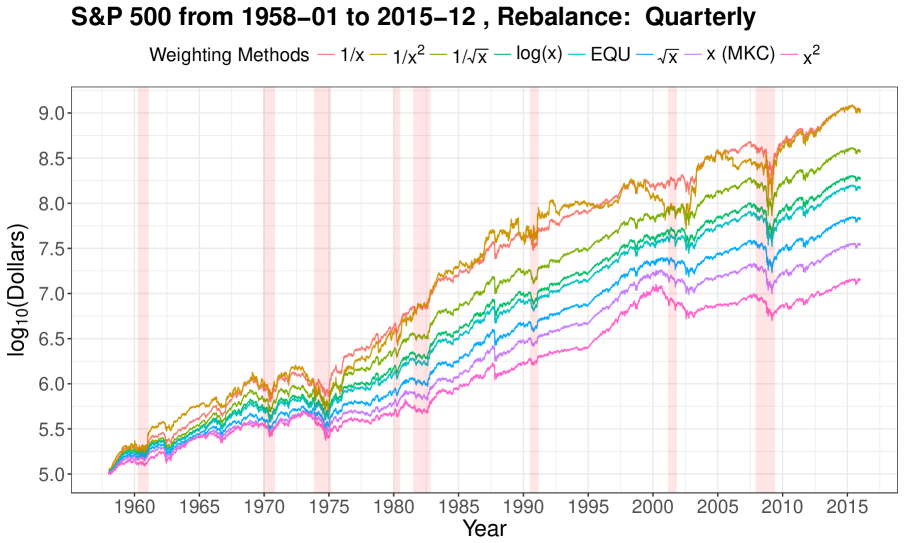
$1/x^{2}$	$1/x$	$1/\sqrt{x}$	$\log\left(x\right)$	EQU	$\sqrt{x}$	$x$	$x^{2}$
$1.054 bil	$1.081 bil	$377.268 mil	$187.874 mil	$148.360 mil	$67.326 mil	$34.959 mil	$14.113 mil

Table 17: Ending balance on 12/31/15.

We next consider annual rebalancing. Figure 7 below displays the cumulative returns calculated from 1958 to 2015 of the equally weighted S&P 500 portfolio (EQU) and the seven portfolios given by the Tukey transformations ($1/x^{2},\,\,1/x,\,\,1/\sqrt{x},\,\,\text{log}(x),\,\,\sqrt{x},\,\,x,\,\,x^{2}$), where $x$ is the market capitalization weighted portfolio, and the portfolios are rebalanced annually.

Figure 7: Tukey transformation ladder with yearly rebalancing from 1958 to 2015.

The cumulative returns displayed in Figure 7 are reproduced in Table 18 below.

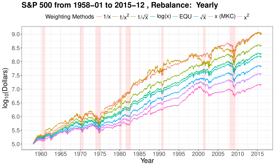
$1/x^{2}$	$1/x$	$1/\sqrt{x}$	$\log\left(x\right)$	EQU	$\sqrt{x}$	$x$	$x^{2}$
$999.798 mil	$1.084 bil	$381.412 mil	$190.942 mil	$151.005 mil	$69.160 mil	$36.106 mil	$14.692 mil

Table 18: Ending balance on 12/31/15.

We conclude by summarizing the findings of Figures 6 and 7 for the $1/x^{2}$ portfolio. When rebalanced quarterly, the balance of the $1/x^{2}$ portfolio on 12/31/15 is $1.054 billion. When rebalanced annually, the value of the $1/x^{2}$ portfolio on 12/31/15 $999.798 million. The $1.477 billion figure for the ending balance on 12/31/15 for the monthly rebalanced $1/x^{2}$ portfolio (Table 6) exceeds that of both quarterly rebalancing (Table 17) and of annual rebalancing (Table 18).

APPENDIX C

Results of Bootstrap for Random $N$

This Appendix displays the bootstrapped distributions for fixed $N$ for a seven different values of $N$
($N=20,50,100,200,300,400,500$). The results herein are presented to support our findings in Section 6.2 of the main manuscript.

C.1: $N=20$

Figure 8: The bootstrap distribution for $N=20$.

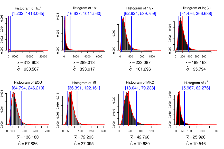
	mean	median	sd	q5th	q95th	q1th	q99th
$1/x^{2}$	313.608	53.904	930.567	1.202	1413.065	0.206	4117.225
$1/x$	289.013	156.083	393.917	16.627	1011.560	6.456	1903.231
$1/\sqrt{x}$	233.087	192.686	161.296	62.624	539.759	38.731	805.649
$\log\left(x\right)$	189.163	169.573	95.794	74.476	366.688	53.044	509.182
EQU	138.180	127.712	57.886	64.794	246.210	48.370	322.390
$\sqrt{x}$	72.293	68.113	27.095	36.391	122.161	27.708	155.877
$x$	42.768	39.249	19.680	18.041	79.238	12.319	108.881
$x^{2}$	25.926	21.423	19.546	5.987	62.276	3.236	100.276

Table 19: Sample statistics for the cumulative return on 12/31/15 for $N=20$, calculated from 20,000 simulations. All numbers are in million USD.

C.2: $N=50$

Figure 9: The bootstrap distribution for $N=50$.

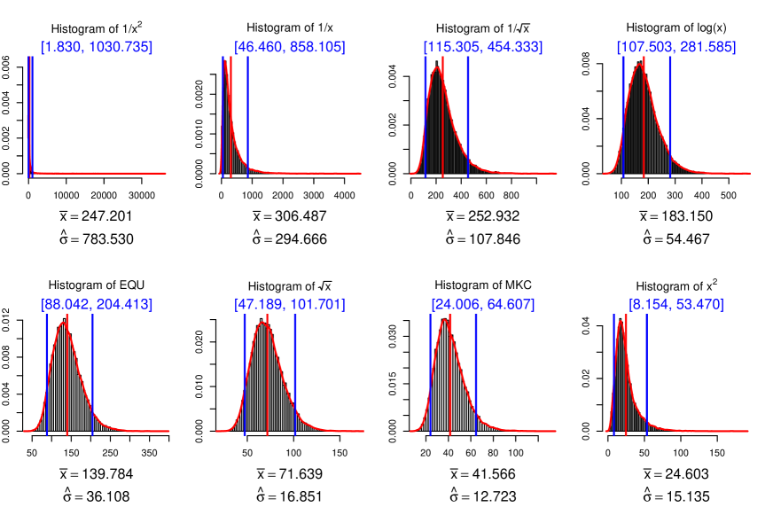
	mean	median	sd	q5th	q95th	q1th	q99th
$1/x^{2}$	247.201	51.832	783.530	1.830	1030.735	0.476	3127.920
$1/x$	306.487	216.857	294.666	46.460	858.105	22.401	1444.515
$1/\sqrt{x}$	252.932	233.828	107.846	115.305	454.333	84.473	592.379
$\log\left(x\right)$	183.150	176.354	54.467	107.503	281.585	86.982	342.475
EQU	139.784	135.746	36.108	88.042	204.413	73.265	243.520
$\sqrt{x}$	71.639	70.064	16.851	47.189	101.701	39.665	118.217
$x$	41.566	39.805	12.723	24.006	64.607	18.968	79.438
$x^{2}$	24.603	20.977	15.135	8.154	53.470	5.084	79.391

Table 20: Sample statistics for the cumulative return on 12/31/15 for $N=50$, calculated from 20,000 simulations. All numbers are in million USD.

C.3: $N=100$

Figure 10: The bootstrap distribution for $N=100$.

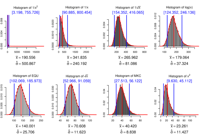
	mean	median	sd	q5th	q95th	q1th	q99th
$1/x^{2}$	190.556	55.298	500.867	3.198	755.726	0.902	2128.342
$1/x$	341.835	282.757	240.192	90.885	800.454	53.339	1196.739
$1/\sqrt{x}$	265.962	254.665	81.086	154.352	416.065	123.279	503.724
$\log\left(x\right)$	179.064	175.209	37.324	124.352	246.136	107.527	281.018
EQU	140.001	137.717	25.706	102.069	185.973	89.326	209.102
$\sqrt{x}$	70.608	69.817	11.623	52.966	91.059	47.388	101.690
$x$	40.420	39.613	8.838	27.513	56.122	23.357	65.239
$x^{2}$	23.261	20.712	11.427	9.630	45.112	6.529	61.034

Table 21: Sample statistics for the cumulative return on 12/31/15 for $N=100$, calculated from 20,000 simulations. All numbers are in million USD.

C.4: $N=200$

Figure 11: The bootstrap distribution for $N=200$.

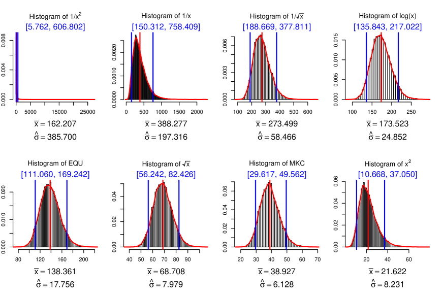
	mean	median	sd	q5th	q95th	q1th	q99th
$1/x^{2}$	162.207	64.156	385.700	5.762	606.802	2.036	1508.764
$1/x$	388.277	347.982	197.316	150.312	758.409	105.384	1039.324
$1/\sqrt{x}$	273.499	267.685	58.466	188.669	377.811	162.252	434.943
$\log\left(x\right)$	173.523	171.956	24.852	135.843	217.022	122.656	238.693
EQU	138.361	137.392	17.756	111.060	169.242	101.419	184.743
$\sqrt{x}$	68.708	68.347	7.979	56.242	82.426	51.664	89.029
$x$	38.927	38.550	6.128	29.617	49.562	26.363	54.955
$x^{2}$	21.622	20.345	8.231	10.668	37.050	7.854	46.815

Table 22: Sample statistics for the cumulative return on 12/31/15 for $N=200$, calculated from 20,000 simulations. All numbers are in million USD.

C.5: $N=300$

Figure 12: The bootstrap distribution for $N=300$.

	mean	median	sd	q5th	q95th	q1th	q99th
$1/x^{2}$	159.638	73.879	279.421	8.289	579.868	3.437	1324.234
$1/x$	416.421	386.993	173.709	190.130	739.815	140.194	959.616
$1/\sqrt{x}$	276.489	272.826	48.261	203.669	361.378	181.529	405.815
$\log\left(x\right)$	169.939	168.763	19.869	139.163	204.070	128.248	220.758
EQU	136.784	136.063	14.470	114.274	161.798	106.171	173.457
$\sqrt{x}$	67.285	67.017	6.456	57.212	78.367	53.540	83.961
$x$	37.977	37.692	4.966	30.388	46.660	27.711	50.785
$x^{2}$	20.774	19.895	6.685	11.426	33.052	8.649	40.593

Table 23: Sample statistics for the cumulative return on 12/31/15 for $N=300$, calculated from 20,000 simulations. All numbers are in million USD.

C.6: $N=400$

Figure 13: The bootstrap distribution for $N=400$.

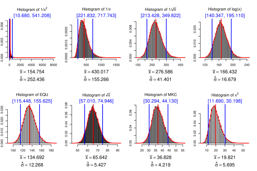
	mean	median	sd	q5th	q95th	q1th	q99th
$1/x^{2}$	154.754	78.818	252.436	10.680	541.208	4.452	1185.654
$1/x$	430.017	406.943	155.266	221.832	717.743	172.303	901.348
$1/\sqrt{x}$	276.586	273.788	41.401	213.428	349.822	192.470	385.304
$\log\left(x\right)$	166.432	165.592	16.679	140.347	195.110	130.664	208.605
EQU	134.692	134.124	12.268	115.448	155.625	108.059	165.356
$\sqrt{x}$	65.642	65.399	5.427	57.010	74.946	54.037	79.065
$x$	36.828	36.594	4.219	30.294	44.130	27.915	47.650
$x^{2}$	19.821	19.133	5.695	11.690	30.198	9.375	35.838

Table 24: Sample statistics for the cumulative return on 12/31/15 for $N=400$, calculated from 20,000 simulations. All numbers are in million USD.

C.7: $N=500$

Figure 14: The bootstrap distribution for $N=500$.

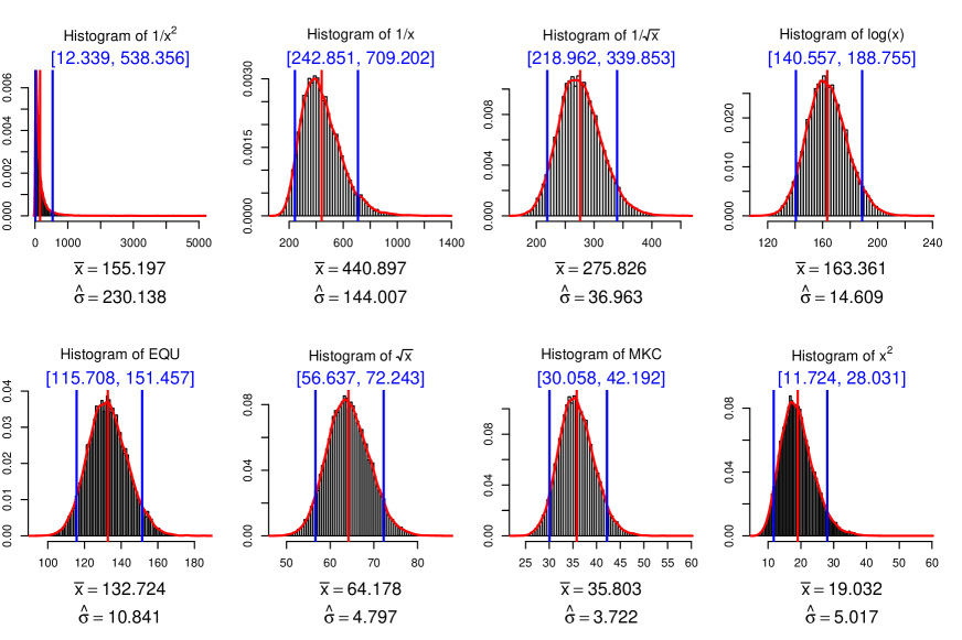
	mean	median	sd	q5th	q95th	q1th	q99th
$1/x^{2}$	155.197	83.330	230.138	12.339	538.356	5.825	1057.348
$1/x$	440.897	420.618	144.007	242.851	709.202	189.991	860.461
$1/\sqrt{x}$	275.826	273.563	36.963	218.962	339.853	199.851	372.607
$\log\left(x\right)$	163.361	162.654	14.609	140.557	188.755	131.992	199.961
EQU	132.724	132.275	10.841	115.708	151.457	109.453	159.636
$\sqrt{x}$	64.178	63.957	4.797	56.637	72.243	53.787	76.126
$x$	35.803	35.583	3.722	30.058	42.192	27.859	45.267
$x^{2}$	19.032	18.518	5.017	11.724	28.031	9.607	33.065

Table 25: Sample statistics for the cumulative return on 12/31/15 for $N=500$, calculated from 20,000 simulations. All numbers are in million USD.

APPENDIX D

Value of S&P 500 Portfolio over the 1980-2015, 1990-2015, and 2000-2015 horizons

In this Appendix, we show that the returns of the eight portfolios under consideration precisely follow the order of the Tukey transformational ladder for three additional time horizons: 1980-2015, 1990-2015, and 2000-2015.
We first consider the 1980-2015 horizon. We invest $272,028 on 1/2/80 (the equivalent of $100,000 in 1958 dollars) and let each portfolio grow until 12/31/15. The cumulative returns are displayed below.

Figure 15: Cumulative $\text{log}_{10}$ returns (from 1980-2015) for the EQU portfolio and the seven Tukey transformational ladder portfolios. The calculation assumes that $272,028 is invested on 1/2/80 and is left to grow until 12/31/15.

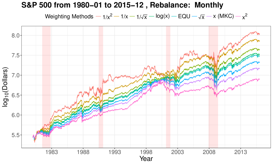
The cumulative returns on 12/31/15 displayed in the above Figure are reproduced in Table 26 below.

$1/x^{2}$	$1/x$	$\sqrt{x}$	$\log\left(x\right)$	EQU	$\sqrt{x}$	$x$	$x^{2}$
$107.967 mil	$72.113 mil	$ 43.637 mil	$ 33.160 mil	$ 30.086 mil	$ 21.066 mil	$14.730 mil	$ 7.875 mil

Table 26: The cumulative returns for the EQU portfolio and the seven Tukey transformational ladder portfolios. The calculation assumes that $272,028 is invested on 1/2/80 and is left to grow until 12/31/15.

We now consider the 1990-2015 time horizon. We invest $445,455 on 1/2/90 (the equivalent of $100,000 in 1958 dollars) and let the portfolios grow until 12/31/15. The results are displayed in Figure 16 below.

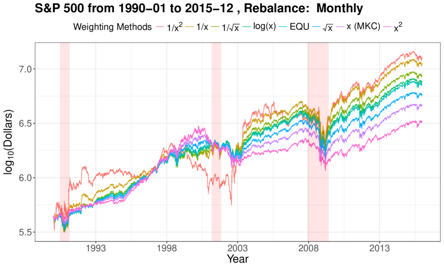
Figure 16: Cumulative $\text{log}_{10}$ returns (from 1990-2015) for the EQU portfolio and the seven Tukey transformational ladder portfolios. The calculation assumes that $445,455 is invested on 1/2/90 and is left to grow until 12/31/15.

The cumulative returns displayed in Figure 16 are reproduced in Table 27 below

$1/x^{2}$	$1/x$	$\sqrt{x}$	$\log\left(x\right)$	EQU	$\sqrt{x}$	$x$	$x^{2}$
$12.527 mil	$11.041 mil	$8.646 mil	$7.582 mil	$7.197 mil	$5.808 mil	$4.608 mil	$3.242 mil

Table 27: The cumulative returns for the EQU portfolio and the seven Tukey transformational ladder portfolios. The calculation assumes that $445,455 is invested on 1/2/90 and is left to grow until 12/31/15.

Finally, we consider the 2000-2015 time horizon. We invest $590,210 on 1/2/00 (the equivalent of $100,000 in 1958 dollars) and let the portfolios grow until 12/31/15. We display the results in Figure 17 below.

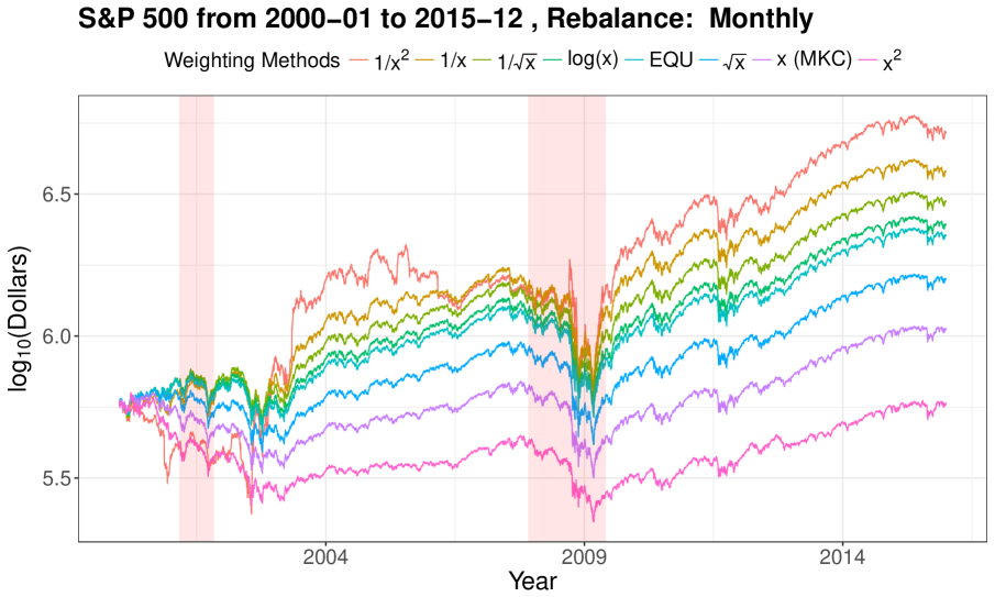
Figure 17: Cumulative $\text{log}_{10}$ returns (from 2000-2015) for the EQU portfolio and the Tukey transformational ladder portfolios. The calculation assumes that $590,210 is invested on 1/2/00 and is left to grow until 12/31/15.

The cumulative returns displayed in Figure 17 are produced in Table 28 below

$1/x^{2}$	$1/x$	$\sqrt{x}$	$\log\left(x\right)$	EQU	$\sqrt{x}$	$x$	$x^{2}$
$5.176 mil	$3.762 mil	$2.952 mil	$2.446 mil	$2.243 mil	$ 1.572 mil	$1.048 mil	$.570 mil

Table 28: The cumulative returns for the EQU portfolio and the seven Tukey transformational ladder portfolios. The calculation assumes that $590,210 is invested on 1/2/00 and is left to grow until 12/31/15.

In conclusion, tables 26, 27, 28 each show that the portfolio returns precisely follow the order of the Tukey transformational ladder.

Supplementary Materials For purposes of replication, all code used in this work can be found online on the following GitHub repository: https://github.com/yinsenm/Tukeytransforms.

Short CVs

Philip Ernst is an Assistant Professor at Rice University’s Department of Statistics. He received his Ph.D. in 2014 from The Wharton School of the University of Pennsylvania and joined the Rice faculty the same year. He holds a M.A. in Statistics from The Wharton School of the University of Pennsylvania and a B.A. in Statistics cum laude from Harvard University. His research interests are mathematical finance, applied probability, and statistical theory. In the past three years, he has published four articles in mathematical finance (Ernst et al., (2014), Ernst and Shepp, (2015), Ernst, (2017), Ernst et al., (2017)).

James R. Thompson is Emeritus Noah Harding Professor and Research Professor of Statisitics at Rice University. He holds a BE in Chemical Engineering from Vanderbilt and a doctorate in Mathematics from Princeton. He is the author or co-author of 14 books and over 100 articles. A Fellow of the ASA, the IMS and the ISI, he is recipient of the Army’s Wilks Award for contributions related to National Defense. He has held adjunct professor rank at the M.D. Anderson Cancer Center and the UTS School of Public Health. His primary current interests are in epidemiology, oncology, business, and quality control.

Yinsen Miao is a second year Ph.D. student in the Department of Statistics at Rice University. His research interests include portfolio optimization, statistical machine learning, convex optimization, and Bayesian models. His research focuses on developing statistical algorithms for sparse data. He received his M.A. in Statistics from Rice University and his bachelor degree from Minzu University of China.

References

- Baggett and Thompson, (2007) Baggett, L. and Thompson, J. R. (2007). Everyman’s MaxMedian rule for portfolio management. In 13th army conference on applied statistics.
- Banz, (1981) Banz, R. (1981). The relationship between return and market value of common stocks. Journal of Financial Economics, 9:3–18.
- Bloomfield et al., (1977) Bloomfield, T., Leftwich, R., and Long, J. (1977). Portfolio strategies and performance. Journal of Financial Economics, 5:201–218.
- Bogle, (2000) Bogle, J. (2000). Common Sense on Mutual Funds: New Imperatives for the Intelligent Investor. John Wiley & Sons.
- Chan et al., (1996) Chan, L. K., Jegadeesh, N., and Lakonishok, J. (1996). Momentum strategies. The Journal of Finance, 51(5):1681–1713.
- DeMiguel et al., (2009) DeMiguel, V., Garlappi, L., and Uppal, R. (2009). Optimal versus naive diversification: how inefficient is the 1/N portfolio strategy? Review of Financial Studies, 22(5):1915–1953.
- Ernst, (2017) Ernst, P. (2017). On the arbitrage price of European call options. Stochastic Models, 33(1):48–58.
- Ernst et al., (2014) Ernst, P. A., Foster, D. P., and Shepp, L. A. (2014). On optimal retirement. Journal of Applied Probability, 51(2):333–345.
- Ernst et al., (2017) Ernst, P. A., Rogers, L. C. G., and Zhou, Q. (2017). The value of foresight. Stochastic Processes and their Applications.
- Ernst and Shepp, (2015) Ernst, P. A. and Shepp, L. A. (2015). Revisiting a theorem of LA Shepp on optimal stopping. Communications on Stochastic Analysis, 9(3):419–423.
- Fama and French, (1992) Fama, E. and French, K. (1992). Common risk factors in the returns on stocks and bonds. Journal of Finance, 47:427–465.
- Franck et al., (2013) Franck, A., Walter, A., and Witt, J. F. (2013). Momentum strategies of German mutual funds. Financial Markets and Portfolio Management, 27(3):307–332.
- Goetzmann and Massa, (2002) Goetzmann, W. N. and Massa, M. (2002). Daily momentum and contrarian behavior of index fund investors. Journal of Financial and Quantitative Analysis, 37(03):375–389.
- Hirshleifer, (2001) Hirshleifer, D. (2001). Investor psychology and asset pricing. Journal of Finance, 56:1533–1597.
- Horowitz et al., (2000) Horowitz, J., Loughran, T., and Savin, N. (2000). Three analyses of the firm size premium. Journal of Empirical Finance, 7:143–153.
- Jacobs et al., (2014) Jacobs, H., Muller, S., and Weber, M. (2014). How should individual investors diversify? An empirical evaluation of alternative asset allocation policies. Journal of Financial Markets, 19:62–85.
- Kadan and Liu, (2014) Kadan, O. and Liu, F. (2014). Performance evaluation with high moments and disaster risk. Journal of Financial Economics, 113:131–155.
- Thompson, (2011) Thompson, J. R. (2011). Empirical Model Building: Data, Models, and Reality. John Wiley & Sons.
- Treynor, (2005) Treynor, J. (2005). Why market valuation indifferent indexing works. Financial Analysts Journal, 61(5):65–69.
- Tukey, (1962) Tukey, J. (1962). The future of data analysis. Annals of Mathematical Statistics, 33(1):1–67.
- Tukey, (1977) Tukey, J. (1977). Exploratory Data Analysis. Addison-Wesley.
- van Dijk, (2011) van Dijk, M. (2011). Is size dead? a review of the size effect in equity returns. Journal of Banking and Finance, 35:3263–3274.
- Wojciechowski and Thompson, (2006) Wojciechowski, W. and Thompson, J. R. (2006). Market truths: theory versus empirical simulations. Journal of Statistical Computation and Simulation, 76(5):385–395.
- Yao, (2012) Yao, Y. (2012). Momentum, contrarian, and the January seasonality. Journal of Banking & Finance, 36(10):2757–2769.