How local is the information in tensor networks of matrix product states and entangled pairs states

Abstract

Two dimensional tensor networks such as projected entangled pairs states (PEPS) are generally hard to contract. This is arguably the main reason why variational tensor network methods in 2D are still not as successful as in 1D. However, this is not necessarily the case if the tensor network represents a gapped ground state of a local Hamiltonian; such states are subject to many constraints and contain much more structure. In this paper we introduce an approach for approximating the expectation value of a local observable in ground states of local Hamiltonians that are represented by PEPS tensor-networks. Instead of contracting the full tensor-network, we try to estimate the expectation value using only a local patch of the tensor-network around the observable. Surprisingly, we demonstrate that this is often easier to do when the system is frustrated. In such case, the spanning vectors of the local patch are subject to non-trivial constraints that can be utilized via a semi-definite program to calculate rigorous lower- and upper-bounds on the expectation value. We test our approach in 1D systems, where we show how the expectation value can be calculated up to at least 3 or 4 digits of precision, even when the patch radius is smaller than the correlation length.

I Introduction

Variational tensor-network methods Orús (2014) provide a promising way for understanding the low-temperature physics of many-body condensed matter systems. In particular, they seem suitable for studying the ground states of highly frustrated systems, where the sign problem limits many of the quantum Monte Carlo approaches. The best-known and by far the most successful tensor-network method is the Density Matrix Renormalization Group (DMRG) algorithm White (1992, 1993). It has revolutionized our ability to numerically probe strongly correlated systems in 1D, often providing results up to machine precision. Today, it is generally believed to be the optimal method for finding ground states of 1D lattice models.

DMRG can be viewed as a variational algorithm for minimizing the energy of the system over the manifold of Matrix Product States (MPS) Östlund and Rommer (1995); Rommer and Östlund (1997). These are special types of tensor-network with a linear, 1D structure. In 2D and beyond, several generalizations of this approach are possible. Arguably, the most natural generalization is Projected Entangled Pairs State (PEPS) tensor network Verstraete and Cirac (2004); Verstraete et al. (2008), which was introduced by Verstraete and Cirac in 2004 Verstraete and Cirac (2004), but was also used earlier under different names such as “vertex matrix product ansatz” in LABEL:ref:SM1998-DMRG-CFT, “tensors product form ansatz” (TPFA) in LABEL:ref:HOK1999:NRG2D, and “tensor product state” (TPS) in LABEL:ref:NHYOMAG2001-TPS. It is the main tensor-network that we consider in this paper. Other constructions include Tree Tensor Networks Shi et al. (2006), Multi-scale Entanglement Renormalization ansatz (MERA) Vidal (2008), String bond states Schuch et al. (2008), and the recently introduced Projected Entangled Simplex States (PESS) Xie et al. (2014), to name a few. These tensor-networks have proven a vital theoretical tool for understanding the physics of 2D lattice systems and in particular their entanglement structure. However, as a numerical method for studying highly frustrated 2D quantum systems, they still face substantial challenges which limit their applicability. In most cases, the best results are still obtained either by DMRG, in which a 1D MPS wraps around the 2D surface, or by quantum Monte Carlo methods.

There are several reasons for this qualitative difference between 1D and 2D systems. The most important one is the computational cost of contracting 2D tensor networks. While this cost scales linearly in the 1D case, it is exponential for 2D and above. Formally, this is reflected in the fact that contracting a PEPS is #P-hard Schuch et al. (2007), which is at least NP-hard. To overcome this exponential hurdle, many approximation schemes have been devised. For example, in the original PEPS paper, the network is contracted column by column from left to right, by treating the tensors of a column as matrix product operators (MPO) that act on a MPS that represents the contracted part of the network. Throughout the contraction, the bond dimension of the MPS is truncated to some prescribed $D^{\prime}$, which introduces some errors (for details, see Refs. Verstraete and Cirac, 2004; Verstraete et al., 2008). Other approximate methods include, for example, the Corner Transfer Matrix (CTM) Nishino and Okunishi (1996); Orús and Vidal (2009); Orús (2012); Vanderstraeten et al. (2015), coarse-graining by tensor Renormalization Levin and Nave (2007); Xie et al. (2009); Zhao et al. (2010); Xie et al. (2012), the single layer method Pižorn et al. (2011) and other variants.

While all of the above methods are physically motivated, none of them are rigorous. And to some extent they all produce uncontrolled approximations, even when dealing with the ground state itself. Moreover, while their computational cost is now polynomial in the bond dimension and the particle number, it still scales badly, which limits their practical use to small systems/resolutions (state of the art now days is around $15\times 15$ sites with $D=6$  Lubasch et al. (2014a)). This has led some researchers to develop the popular simulation framework, known as the “simple update” method, in which one completely abandons the contraction of the 2D network during the variational procedure Jiang et al. (2008), essentially approximating the environment of a local tensor by a product state. While this allows for much higher bond dimensions and is often successful for translationally invariant systems, it may produce poor results for systems that approach critically; see, for example, the analysis in Refs. Lubasch et al., 2014b, a.

In this paper we introduce a new approach for approximating the expectation values of local observables in a 2D PEPS tensor-network. Instead of contracting the full tensor network (or approximating such full contraction), we aim at approximating the expectation value using only the information inside a local patch of the tensor-network around the local observable. Clearly, this approach will fail for general PEPS since they often contain highly non-local correlations. However, as we shall demonstrate, such an approach can produce non-trivial results when applied to PEPS that are ground states of gapped local Hamiltonains. Indeed, it is known that such states exhibit strong properties of locality, such as exponential decay of correlations Hastings (2004); Hastings and Koma (2006); Nachtergaele and Sims (2006) and local reversibility Kuwahara et al. (2015), and are therefore subject to many constraints to which arbitrary PEPS are not. Moreover, we have the local Hamiltonian at our hands, which can be used to evaluate the local expectation value. Our goal in this paper is to show that for these states, very good approximations for the local expectation values can be derived only from a local patch.

We identify two possible mechanisms for such approximations, which form the basis for two numerical algorithms. In both algorithms, the entire calculation is local and can therefore be done, in principle, efficiently. Moreover, both algorithms provide rigorous upper- and lower- bounds on the expectation value. While we usually cannot give rigorous bound on the distance between these bounds, we demonstrate numerically that this distance – and hence the error in our approximation – can be surprisingly small.

The first algorithm, which we call the ‘basic algorithm’, is expected to give good results in the case of frustration-free gapped systems. The second one, which we call the ‘commutator gauge optimization’ (CGO) algorithm, works only for frustrated systems by utilizing the additional constraints in these systems. It does not rely directly on the existence of a gap, and may work even when considering patches of the PEPS that are much smaller than the correlation length. We numerically demonstrate both algorithms using MPS in 1D systems. Regarding the title of this paper, our findings suggest that when the PEPS/MPS tensor-network represents a frustrated ground state, the information about the local expectation value is largely encoded locally in the neighborhood of the observable.

We would like to stress from the start that the algorithms we present are not practical, and can only be used in 1D in a reasonable time. Their main goal, which is the main goal of this paper, is to illustrate the locality of information in MPS/PEPS representations of gapped ground states. Nevertheless, we strongly believe that the mechanisms behind these algorithms can be further exploited and turned into practical heuristic algorithms. We leave this interesting research direction for further work.

The organization of this paper is as follows. In Sec. II we formally define the problem we wish to solve and the assumptions we are using. In Sec. III we introduce the basic algorithm to solve the problem, and in Sec. IV we introduce the CGO algorithm. In Sec. V we present the results of the 1D numerical tests, and in Sec. VI we discuss the results and offer our conclusions.

II Statement of the problem

Our construction involves PEPS and MPS tensor networks. For the exact definition and review of these tensor networks (and tensor networks in general), we refer the reader to Refs. Orús, 2014; Verstraete et al., 2008.

We are given a local Hamiltonian $H=\sum_{i}h_{i}$ that is defined on a system of $N\times N$ spins of local dimension $d$ that sit on a 2D rectangular lattice, which can be either open or with periodic boundary conditions. The local terms $h_{i}$ have $\mathcal{O}(1)$ bounded norms, and are assumed to be working on nearest-neighbors only. We further assume that $H$ is gapped, with a unique ground state $|\Omega\rangle$ that is exactly described by a PEPS with bond dimension $D=\mathcal{O}(1)$. While in practice this is rarely the case, and $D$ may have to be exponentially large in order for the PEPS to exactly describe the ground state, it is expected that a $D=\mathcal{O}(1)$ bond dimension should give very good approximations to a gapped ground state. For the sake of clarity we first assume that the $D=\mathcal{O}(1)$ description is exact and return to discuss this assumption in Sec. IV.4.

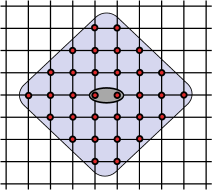
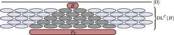
Given a local observable $B$ that acts on, say, 2 neighboring spins on the lattice, our task is to approximate $\langle B\rangle:=\langle\Omega|B|\Omega\rangle$ using only a local patch of the PEPS around $B$. Specifically, the local patch is defined by a ball $L$ of radius $\ell$ around $B$. $L$ contains all the sites on the lattice that can be connected to the support of $B$ using at most $\ell$ steps on the lattice. We let $L^{c}$ denote the complement region of $L$ that contains all the spins outside of $L$. An example of the local ball $L$ for $\ell=3$ is given in Fig. 1.

Figure 1: An example of a ball $L$ of radius $\ell=3$ around a 2-local operator. The region $L$ consists of the $32$ spins that are marked by red dots.

Without loss of generality, we will assume that $B$ is normalized so that $\|B\|=1$; all of our results can be applied to the general case with a simple rescaling.

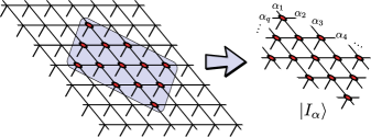
Consider then the PEPS representation of $|\Omega\rangle$, and let $\alpha=(\alpha_{1},\alpha_{2},\ldots,)$ be the set of virtual indices that connect the spins in $L$ to those outside of it. As illustrated in Fig. 2, it defines the following decomposition of $|\Omega\rangle$:

$$|\Omega\rangle=\sum_{\alpha}|O_{\alpha}\rangle\otimes|I_{\alpha}\rangle\,.$$ (1)

Above, $\{|O_{\alpha}\rangle\}$, $\{|I_{\alpha}\rangle\}$ are states that are defined by the PEPS tensor-network outside and inside $L$ respectively. The sets of vectors $\{|O_{\alpha}\rangle\}$, $\{|I_{\alpha}\rangle\}$ are not necessarily orthogonal between themselves, nor are they normalized, but we assume that both $\{|I_{\alpha}\rangle\}$ and $\{|O_{\alpha}\rangle\}$ are linearly independent among themselves. This is a stronger condition than the injectivity condition for the PEPS, in which only $\{|I_{\alpha}\rangle\}$ have to be linearly independent Perez-Garcia et al. (2008), but as injectivity, we expect it to hold for generic PEPS. We define $V_{L}:=\mathop{\rm span}\nolimits\{|I_{\alpha}\rangle\}$ and let $\rho_{L}$ denote the reduced density matrix of $|\Omega\rangle$ on $L$, which lives in the subspace $V_{L}$. Note that from our assumptions on $\{|I_{\alpha}\rangle\}$ and $\{|O_{\alpha}\rangle\}$ it follows that $V_{L}=\mathrm{Im}\rho_{L}$. We let $q:=\dim V_{L}$, which is equal to the size of the range in which the composite index $\alpha=(\alpha_{1},\alpha_{2},\ldots)$ runs. Notice that $q=D^{\mathcal{O}(|\partial L|)}$, reflecting the fact that $|\Omega\rangle$ satisfies an area law.

Figure 2: Illustration of the decomposition $|\Omega\rangle=\sum_{\alpha}|O_{\alpha}\rangle\otimes|I_{\alpha}\rangle$, defined by a ball $L$ and the underlying PEPS. The boundary of $L$ cuts the PEPS virtual links $\alpha=(\alpha_{1},\alpha_{2},\ldots,\alpha_{q})$ and defines the outer states $\{|O_{\alpha}\rangle\}$ and the inner states $\{|I_{\alpha}\rangle\}$, which are described on the right part of the figure. The inner vectors $\{|I_{\alpha}\rangle\}$ and the subspace $V_{L}$ that they span can be efficiently calculated.

Clearly, if we knew $\rho_{L}$ we could calculate $\langle B\rangle$ from $\langle B\rangle=\langle\Omega|B|\Omega\rangle=\mathop{\rm Tr}\nolimits_{L}(\rho_{L}B)$. However, directly estimating $\rho_{L}$ involves the contraction of the full network, which is exactly what we are trying to avoid. Instead, since the radius $\ell$ is assumed to be small, we can easily calculate $V_{L}:=\mathop{\rm span}\nolimits\{|I_{\alpha}\rangle\}$. Can we estimate $\langle B\rangle$ using only $V_{L}$ and the fact that $|\Omega\rangle$ is the ground state of $H$? Formally, we ask:

Problem 1

Given a local observable $B$, a ball $L$ of radius $\ell$ around it, and the corresponding subspace $V_{L}$, find a range $[b_{min},b_{max}]$, as narrow as possible, such that $\langle B\rangle\in[b_{min},b_{max}]$.

We offer two algorithms to tackle this problem. The first, which we call the ‘basic algorithm’, is expected to work well when the system is gapped, and is suitable mostly for frustration-free systems. The second, which we call ‘the commutators gauge optimization’ algorithm, is much more powerful and applies only for frustrated systems. It relies on the assumption that $|\Omega\rangle$ with $D=\mathcal{O}(1)$ is described by a PEPS and therefore satisfies an area law (this, in turn, can also be attributed to the existence of a gap). We begin with the basic algorithm.

III The basic algorithm

Let $P_{V}$ be the projector into the subspace $V_{L}$, and define $B_{L}:=P_{V}BP_{V}$. Then as $\rho_{L}=P_{V}\rho_{L}P_{V}$, we get from the cyclicity of the trace that $\langle B\rangle=\mathop{\rm Tr}\nolimits(B\rho_{L})=\mathop{\rm Tr}\nolimits(BP_{V}\rho_{L}P_{V})=\mathop{\rm Tr}\nolimits(P_{V}BP_{V}\rho_{L})=\mathop{\rm Tr}\nolimits(B_{L}\rho_{L})$. Equivalently, $\langle B\rangle=\langle\Omega|B_{L}|\Omega\rangle$. Therefore, if $b_{1}\leq b_{2}\leq\ldots\leq b_{q}$ are the eigenvalues of $B_{L}$ in the subspace $V_{L}$, then $\langle B\rangle\in[b_{1},b_{q}]$. The basic algorithm then simply calculates the largest and the smallest eigenvalues of $B_{L}$ in the $V_{L}$ subspace and use these as lower- and upper- bounds to $\langle B\rangle$.

Intuitively, when the system is gapped, we expect the range $[b_{1},b_{q}]$ to narrow down as $\ell\to\infty$ for the following reason. Every $\alpha=(\alpha_{1},\ldots,\alpha_{q})$ can be seen as a specific boundary condition for a restricted system on the ball $L$, and as the system is gapped, we expect the effect of these boundary conditions to be negligible. Hence, we expect that for every $|I_{\alpha}\rangle$, we have $\langle I_{\alpha}|B|I_{\alpha}\rangle/\|I_{\alpha}\|^{2}\to\langle B\rangle$ as $\ell\to\infty$, and similarly for any linear combination of the $|I_{\alpha}\rangle$ vectors. In particular this means that the eigenvalues of $B_{L}$ are expected to converge to $\langle B\rangle$. The following lemma shows that this is indeed the case when the eigenvalues of $\rho_{L}$ are not too small.

Lemma 1

Let $\lambda^{2}_{min}$ be the minimal eigenvalue of $\rho_{L}$, and let $b_{1},\ldots,b_{q}$ be the eigenvalues of $B_{L}=P_{V}BP_{V}$ in the subspace $V_{L}$. Then for every $\beta=1,\ldots,q$,

$$|b_{\alpha}-\langle B\rangle|\leq\frac{\|B_{L}\|}{\lambda_{min}^{2}}e^{-\ell/\xi}\,,$$ (2)

where $\xi>0$ is the correlation length of $|\Omega\rangle$.

• The proof is a simple application of the basic idea in the Choi-Jamiołkowski isomorphism, together with the exponential decay of correlation property of gapped ground states Hastings (2004). Let $|b_{1}\rangle,|b_{2}\rangle,\ldots|b_{q}\rangle$ be the eigenvectors of $B_{L}$ in $V_{L}$ that correspond to the eigenvalues $b_{1},b_{2},\ldots,b_{q}$. They constitute an orthonormal basis of $V_{L}$. Let $|\Omega\rangle=\sum_{\alpha}\lambda_{\alpha}|\hat{O}_{\alpha}\rangle\otimes|\hat{I}_{\alpha}\rangle$ be the Schmidt decomposition of $|\Omega\rangle$ with respect to $L$ and $L^{c}$ such that $\rho_{L}=\sum_{\alpha}\lambda^{2}_{\alpha}|\hat{I}_{\alpha}\rangle\langle\hat{I}_{\alpha}|$. Both $\{|b_{\beta}\rangle\}$ and $\{|\hat{I}_{\alpha}\rangle\}$ are orthonormal bases of $V_{L}$, and therefore they are connected by a unitary transformation: $|b_{\beta}\rangle=\sum_{\alpha}U_{\beta\alpha}|\hat{I}_{\alpha}\rangle$. We use it to define a set of (un-normalized) states on the spins of $L^{c}$:

  $$|c_{\beta}\rangle:=\sum_{\gamma}\frac{1}{\lambda_{\gamma}}U^{*}_{\beta\gamma}|\hat{O}_{\gamma}\rangle\,.$$ (3)

  In addition, we define the operator $C_{\beta}:=|c_{\beta}\rangle\langle c_{\beta}|\otimes\mathbbm{1}_{L}$, where $\mathbbm{1}_{L}$ is the identity operator on the spins of $L$. Using these definitions, the following identities are easy to verify:

  $$C_{\beta}|\Omega\rangle =|c_{\beta}\rangle\otimes|b_{\beta}\rangle\,,$$ (4)

  $$\|C_{\beta}\| =\|c_{\beta}\|^{2}=\sum_{\gamma}\frac{1}{\lambda^{2}_{\gamma}}|U_{\beta\gamma}|^{2}\,,$$ (5)

  $$C_{\beta}^{2} =\|c_{\beta}\|^{2}C_{\beta}\,.$$ (6)

  Next, by using the exponential decay of correlations Hastings (2004) and the uniqueness of the ground state, we deduce that

  $$\big{|}\langle\Omega|C_{\beta}B|\Omega\rangle-\langle\Omega|C_{\beta}|\Omega\rangle\cdot\langle\Omega|B|\Omega\rangle\big{|}$$ (7)

  $$\ \leq\|B\|\cdot\|C_{\beta}\|\cdot e^{-\ell/\xi}\,.$$

  Let us analyze the above inequality term by term. First, by Eq. (6) and the fact that $C_{\beta}$ and $B$ commute, $\langle\Omega|C_{\beta}B|\Omega\rangle=\frac{1}{\|c_{\beta}\|^{2}}\langle\Omega|C_{\beta}BC_{\beta}|\Omega\rangle$. But then by Eq. (4), this is equal to $\langle b_{\beta}|B|b_{\beta}\rangle=\langle b_{\beta}|B_{L}|b_{\beta}\rangle=b_{\beta}$. A similar argument shows that $\langle\Omega|C_{\beta}|\Omega\rangle=1$. Substituting this into the LHS of (7), we get $|b_{\beta}-\langle B\rangle|\leq\|B\|\cdot\|C_{\beta}\|\cdot e^{-\ell/\xi}$. Finally, using Eq. (5) and the fact that $\sum_{\gamma}|U_{\beta\gamma}|^{2}=1$ (since $U_{\beta\gamma}$ are the entries of a unitary matrix), proves the lemma.  

Lemma 1 shows that if the smallest eigenvalue of $\rho_{L}$ is lowerbounded by $e^{-c\ell/\xi}$ for some $c<1$, the range $[b_{1},b_{q}]$ should converge to the point $\langle B\rangle$ exponentially fast in $\ell$. This is certainly expected in most 1D ground states that are approximated by an MPS of a constant bond dimension $D$. However, it can hardly happen in 2D, where even if the state is approximated by a PEPS with $D=\mathcal{O}(1)$, the dimension of $V_{L}$ grows at least as $D^{\mathcal{O}(\ell)}$, and consequently, the smallest eigenvalue of $\rho_{L}$ is expected to fall off exponentially like $D^{-\mathcal{O}(\ell)}$. In 3D things are even worse, since $\dim V_{L}$ grows like $D^{\mathcal{O}(\ell^{2})}$.

When the underlying Hamiltonian is frustration-free, $V_{L}$ is a subspace of the groundspace of $H_{L}$, the part of $H$ that is supported on the spins of $L$. In such case, it is easy to see that if the Hamiltonian satisfies the local topological order (LTQO) property Michalakis and Zwolak (2013) (see also LABEL:ref:CMPS2013-LTQO2), then necessarily $|b_{\alpha}-\langle B\rangle|$ decays as a function of $\ell$ (the rate of the decay depends on the particular definition of LTQO). Related to that, Lemma 1 has much in common with Theorem 11 of LABEL:ref:CMPS2013-LTQO2, which shows that parent Hamiltonians of translationally invariant, injective MPS satisfy LTQO.

We conclude this section with a somewhat stronger result than Lemma 1 that holds for frustration-free systems:

Lemma 2

When $|\Omega\rangle$ is the unique ground state of a frustration-free Hamiltonian with an $\mathcal{O}(1)$ spectral gap, then

$$B_{L}|\Omega\rangle=\langle B\rangle|\Omega\rangle+|\delta\rangle\,,$$ (8)

where $\||\delta\rangle\|\leq e^{-\mathcal{O}(\ell)}$. In other words, $|\Omega\rangle$ is an approximate eigenvector of $B_{L}$.

The proof of this lemma is given in the Appendix. Formally, it is at least as strong as Lemma 1 because it can be used to derive Lemma 1 when the system is frustration-free. Indeed, using the notation of the proof of Lemma 1, the lemma can be proved by multiplying inequality (8) by $C_{\beta}$ and then by $\langle c_{\beta}|\otimes\langle\beta_{\beta}|$. But it also seems stronger since it tells us something about the eigenvalues of $B_{L}$ even when $\lambda_{min}^{2}$ is much smaller then $e^{-\ell/\xi}$. To see this, note that (8) implies that

$$\|(B_{L}-\langle B\rangle\mathbbm{1})^{2}|\Omega\rangle\|^{2}=\|\delta\|^{2}\leq e^{-\mathcal{O}(\ell)}\,.$$

If $\{|b_{\beta}\rangle\}$ is the eigenbasis of $B_{L}$ with eigenvalues $b_{1},b_{2},\ldots$, then the above inequality can be written as

$$\|(B_{L}-\langle B\rangle\mathbbm{1})^{2}|\Omega\rangle\|^{2}=\mathop{\rm Tr}\nolimits_{L}\big{[}\rho_{L}(B_{L}-\langle B\rangle\mathbbm{1})^{2}\big{]}$$

$$=\sum_{\beta}\langle b_{\beta}|\rho_{L}|b_{\beta}\rangle(b_{\beta}-\langle B\rangle)^{2}\leq e^{-\mathcal{O}(\ell)}\,.$$ (9)

As $\{\langle b_{\beta}|\rho_{L}|b_{\beta}\rangle\}$ is the probability distribution that corresponds to the measurement of $B_{L}$, we can use Markov inequality to deduce that if we measure $B_{L}$ on $|\Omega\rangle$, then with probability of at least $1-e^{-\mathcal{O}(\ell)}$ we will obtain an eigenvalue of $B_{L}$ that is $e^{-\mathcal{O}(\ell)}$ close to $\langle B\rangle$. This holds regardless of the minimal eigenvalue of $\rho_{L}$. Therefore in cases where the weight of all the eigenvalues of $B_{L}$ in $\rho_{L}$ is of the same order (which can be much much smaller than $e^{-\mathcal{O}(\ell)}$ in 3D), then an exponentially large fraction of them must be exponentially close to $\langle B\rangle$. This does not prove that the range $[b_{min},b_{max}]$ rapidly shrinks, but it supports the intuition that this should generally be the case.

We conclude this section noting that for frustrated systems a similar result to Lemma 2 can be proved using the same techniques that are used to prove the exponential decay of correlations in the frustrated case Hastings (2004): a combination of Lieb-Robinson bounds and a suitable filtering function. In fact, a very similar result was already proven by Hastings in LABEL:ref:Hastings2006-GappedH for the special case when $B$ is a local Hamiltonian term. However, instead of pursuing that direction, we turn to a different algorithm, which turns out to be much more powerful for our problem.

IV The commutator gauge optimization

In this section we introduce the Commutator Gauge Optimization algorithm (CGO for short), which is applicable for frustrated systems. As we shall see, it can be viewed as pair of primal-dual SDP optimization problem. We start with the formulation of the primal optimization problems.

IV.1 Primal problem

Our starting point is the simple observation of the basic algorithm, that the expectation value $\langle B\rangle$ must be inside eigenvalues range $[b_{min},b_{max}]$ of the operator $B_{L}:=P_{V}BP_{V}$. The additional idea is that this must hold for any other operator $K$ for which $\langle K\rangle=\langle B\rangle$. Therefore, if we can find an operator $K$ such that $\langle B\rangle=\langle K\rangle$, then necessarily $\langle B\rangle$ must also be inside the range $[k_{min},k_{max}]$ of the minimal and maximal eigenvalues of $P_{V}KP_{V}$. By optimizing over a subset of such operators, we may significantly narrow down the range in which $\langle B\rangle$ is found. We therefore look for operators, $K_{min},K_{max}$ on $L$ such that

$$\langle\Omega|K_{min}|\Omega\rangle=\langle\Omega|K_{max}|\Omega\rangle=\langle\Omega|B|\Omega\rangle\,,$$ (10)

but at the time, $P_{L}K_{max}P_{L}$ has the smallest possible maximal eigenvalue, and $P_{L}K_{min}P_{L}$ has the largest possible minimal eigenvalue.

How can we find such operators? A very simple yet powerful trick is to look for operators of the form:

$$K_{min} =B+[H,A_{min}], K_{max} =B+[H,A_{max}]\,,$$ (11)

where $A_{min},A_{max}$ are anti-Hermitian such that $K_{min},K_{max}$ are Hermitian. For any eigenstate $|\epsilon\rangle$ of $H$ and for any operator $A$, it is easy to verify that $\langle\epsilon|[H,A]|\epsilon\rangle=0$ and therefore Eq. (10) holds. In that sense $K_{min}$ and $K_{max}$ can be viewed as a different “gauges” of $B$, which have the same expectation value with respect to $|\Omega\rangle$.

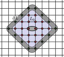
By taking the support of $A_{min},A_{max}$ to be small enough, we can guarantee that $[H,A_{min}]$ and $[H,A_{max}]$ are supported in $L$. Formally, we partition the spins of $L$ into two disjoint subsets, $L=\partial L\cup L_{0}$. Here, $\partial L$ contains the spins in $L$ that are coupled to spins in $L^{c}$ via one or more local terms in $H$, and $L_{0}$ contains the rest of the spins in $L$. An illustration of this decomposition is given in Fig. 3. Letting $H_{L}$ denote the sum of all the local $h_{i}$ terms whose support is inside $L$, we conclude that when the support of $A$ is inside $L_{0}$, then $[H,A]=[H_{L},A]$, and this commutator is supported inside $L$.

Figure 3: The same $\ell=3$ ball $L$ from Fig. 1, now decomposed into the boundary region $\partial L$ (dark gray, green vertices) and the internal region $L_{0}$ (light gray, red vertices).

For a given Hermitian operator $O$, denote by $\lambda_{min}(O),\lambda_{max}(O)$ its minimal/maximal eigenvalues. Then the CGO algorithm can be summarized by the following optimization problem:

Problem 2 (The primal CGO optimization)

Given a local observable $B$, a ground state $|\Omega\rangle$ of a local Hamiltonian $H$ in the form of a PEPS, and a ball $L$ of radius $\ell$ around $B$, calculate

$$k^{(P)}_{max} :=\min_{A}\lambda_{max}\big{(}P_{V}(B+[H_{L},A])P_{V}\big{)}$$ (12)

and

$$k^{(P)}_{min} :=\max_{A}\lambda_{min}\big{(}P_{V}(B+[H_{L},A])P_{V}\big{)}\,.$$ (13)

Above, the optimizations are over all anti-Hermitian operators $A$ that are supported on $L_{0}$.

Two notes are in order. First, the presence of $P_{V}$ in the above equations is crucial, as it is the only place where information about the ground state is entering the problem. Without it, values from other eigenstates of $H$ might worsen our estimate. It is therefore clear why some sort of an area-law is required for CGO to work; if the support of $\rho_{L}$ (i.e., the subspace $V$) is the entire available Hilbert space, there would be nothing in $V_{L}$ to tell us that we are dealing with the ground state and not, say, some other eigenstate of $H$.

Second, when $H$ is frustration free, $P_{V}H_{L}=H_{L}P_{V}=0$ and so $P_{V}(B+[H_{L},A])P_{V}=P_{V}BP_{V}$ for all $A$; the CGO algorithm then simply becomes the basic algorithm.

Before discussing how the optimization Problem 2 can be done in practice, let us introduce its dual.

IV.2 The dual problem

To introduce the dual problem, we begin with the constraint $\langle\Omega|[H_{L},A]|\Omega\rangle=0$, which holds for every $A$ that is supported on the spins in $L_{0}$. Tracing out the spins in $L^{c}$, we get

$$\mathop{\rm Tr}\nolimits(\rho_{L}[H_{L},A])=0\quad\forall A\in\mathop{\rm supp}\nolimits(L_{0})\,.$$ (14)

Using the identity $\mathop{\rm Tr}\nolimits(A[B,C])=\mathop{\rm Tr}\nolimits(C[A,B])$, we arrive at $\mathop{\rm Tr}\nolimits(A[\rho_{L},H_{L}])=0$. Writing $\mathop{\rm Tr}\nolimits=\mathop{\rm Tr}\nolimits_{L_{0}}\mathop{\rm Tr}\nolimits_{\partial L}$, the last equation can be rewritten as $\mathop{\rm Tr}\nolimits_{L_{0}}A\big{(}\mathop{\rm Tr}\nolimits_{\partial L}[\rho_{L},H_{L}]\big{)}=0$. But since $A$ is an arbitrary anti-Hermitian operator on $L_{0}$, it implies that the expression it multiplies has to vanish. We therefore reach the following corollary:

Corollary 3

Let $\rho_{L}$ be the reduced density matrix of an eigenstate of $H$ in the region $L$. Then,

$$\mathop{\rm Tr}\nolimits_{\partial L}[\rho_{L},H_{L}]=0\,.$$ (15)

The above local identity holds for all eigenstates of $H$ and for all regions $L$, regardless of any assumption about a gap or the existence of a PEPS description. When $H$ is frustration free and $\rho_{L}$ is the reduced density matrix of the ground state, it is satisfied trivially since $[\rho_{L},H_{L}]=0$. However, when the system is frustrated, Eq. (15) provides many non-trivial constraints as it holds pointwise on the Hilbert space of $L_{0}$.

Corollary 3 allows us to formulate a dual to the optimization problem given in Problem 2. Instead of optimizing over anti-Hermitian operators $A$, we may optimize over ‘legal’ reduced density matrices, which satisfy Eq. (15). Formally,

Problem 3 (The dual CGO problem)

Given a local observable $B$, a ground state $|\Omega\rangle$ of a local Hamiltonian $H$ in the form of a PEPS, and a ball $L$ of radius $\ell$ around $B$, calculate

$$k^{(D)}_{max} :=\max_{\rho_{L}\in S_{L}}\mathop{\rm Tr}\nolimits(\rho_{L}B)$$ (16)

and

$$k^{(D)}_{min} :=\min_{\rho_{L}\in S_{L}}\mathop{\rm Tr}\nolimits(\rho_{L}B)\,.$$ (17)

Above, $S_{L}$ is the set of all density matrices $\rho_{L}$ in $V_{L}$ [i.e., $\rho_{L}\succeq 0$, $\mathop{\rm Tr}\nolimits(\rho_{L})=1$] that satisfy Eq. (15).

One can prove directly that $k^{(P)}_{max}\geq k^{(D)}_{max}$ and that $k^{(P)}_{min}\leq k^{(D)}_{min}$. We omit the proof since it will follow naturally from viewing these two optimizations as dual semi-definite programs (SDPs), as we shall now do.

IV.3 The commutator gauge optimization as a SDP

The primal CGO problem and its dual can be cast as semi-definite programs. Let us demonstrate it for the upperbound of $\langle B\rangle$; the lowerbound follows similarly. To write (12) as an SDP, note that a number $\lambda$ is an upperbound to all eigenvalues of an operator $O$ iff $\lambda\mathbbm{1}-O\succeq 0$, where $\succeq 0$ stands for non-negative matrix. Then choosing a basis $A_{1},A_{2},\ldots,A_{m}$ for all the anti-Hermitian matrices in $L_{0}$, the optimization over (12) can be written as

minimize: $$b$$ (18)

subject to: $$b\mathbbm{1}-\sum_{i=1}^{m}c_{i}P_{V}[H_{L},A_{i}]P_{V}-P_{V}BP_{V}\succeq 0$$ (19)

Above, the optimization is done over the real numbers $b,c_{1},c_{2},\ldots,c_{m}$. The dual SDP is then

maximize: $$\mathop{\rm Tr}\nolimits(\rho_{L}P_{V}BP_{V})$$ (20)

subject to: $$\rho_{L}\succeq 0,\ \mathop{\rm Tr}\nolimits(\rho_{L}\mathbbm{1})=1,$$ (21)

$$\text{and}\quad\mathop{\rm Tr}\nolimits(\rho_{L}P_{V}[H_{L},A_{i}]P_{V})=0\ \ \forall i$$

which is identical to the optimization in (16). By the weak duality of semi-definite programming, we note that the value in (20) lowerbounds the one in (18), and that in many cases they are identical. In the next section, we present the results of some numerical tests we performed on 1D systems to check the performance of such SDPs.

IV.4 Working with constant bond dimensions

Up to now, we have assumed that the ground state $|\Omega\rangle$ is given exactly as a PEPS with constant bond dimension $D$. However, in virtually all frustrated systems, a constant $D$ can only give an approximation to the ground state. To distinguish the actual PEPS approximation from the exact ground state, we will denote it by $|\Omega_{p}\rangle$. Given that $|\Omega_{p}\rangle$ is only an approximation to the ground state $|\Omega\rangle$, we can only expect $\langle\Omega_{p}|[H,A]|\Omega_{p}\rangle$ to be close to zero, but not completely vanish. Similarly, Eq. (15) is expected to be only approximately satisfied. While this may look merely as an aesthetic defect, it raises a conceptual problem: if $D$ is constant, the dimension of $V_{L}$ increases like $D^{\mathcal{O}(\ell)}$, while the number of constraints in Eq. (15) goes like $d^{\mathcal{O}(\ell^{2})}$. For large enough, yet constant $\ell$, it is expected that Eq. (15) is over-determined, or simply unsatisfiable. From an SDP point of view, we expect the constraints in the primal and the dual problems to become linearly dependent, causing the dual problem not to have any feasible solution and the primal problem to yield infinities.

A practical (though probably not optimal) solution to this is to use only a subset of all possible $A_{i}$ in the SDP procedure. Note that this only relaxes the program in Eq. (20) (and corresponding program for minimum eigenvalue) and hence increases the range $[k^{(D)}_{max},k^{(D)}_{min}]$. One way to do it is to create an increasing list of random $A_{i}$ matrices and feed it to the SDP until they become linearly dependent. As long as the matrices are not linearly dependent and are of a comparable norm, we expect the solution of SDPs (18) and (20) with $P_{V}$ taken from $|\Omega_{p}\rangle$ to produce results that are close to the exact case. The 1D numerical tests that we present in the following section support this intuition.

V Numerical tests

Due to the reduced computational cost, we performed all of our tests on 1D systems whose ground states are described by MPS. Nevertheless, we strongly believe that our conclusions hold also for 2D systems, which we leave for future research.

We analyzed four well-known systems, which we label System-A, System-B, System-C, and System-D. All systems are defined over $N=100$ spins with open boundary conditions. The underlying Hamiltonians are nearest-neighbors with unique ground states and an $\mathcal{O}(1)$ spectral gap and correlation lengths which were calculated numerically. The full details are as follows:

System-A - 1D AKLT.

This is a frustration-free system on spin one particles ($d=3$) Affleck et al. (1987, 1988) given by

$$H_{sysA}:=\sum_{i=1}^{N-1}\big{[}\frac{1}{2}\bm{S}_{i}\cdot\bm{S}_{i+1}+\frac{1}{6}(\bm{S}_{i}\cdot\bm{S}_{i+1})^{2}+\frac{1}{3}\big{]}\,.$$ (22)

The ground state is known analytically, and is described by the AKLT valence bond state, which can be written as a MPS with bond dimension $D=2$. The spectral gap in the thermodynamic limit is $\Delta_{A}\simeq 0.35$ Knabe (1988). The correlation length is $\xi_{A}\simeq 0.9$.

System-B - Transverse Ising model.

This is the classical Ising model equipped with a transverse magnetic field in the $\hat{z}$ direction:

$$H_{sysB}:=-\frac{1}{2\sqrt{1+h^{2}}}\left[\sum_{i=1}^{N-1}S^{x}_{i}S^{x}_{i+1}+h\sum_{i=1}^{N}S^{z}_{i}\right]\,.$$ (23)

At $h=1.0$ the model experiences a phase-transition and the gap closes down. We used $h=1.1$ for which the gap is $\Delta_{B}\simeq 0.07$ and the correlation length is $\xi_{B}\simeq 8.8$.

System-C - Transverse XY model.

This model resembles the transverse Ising model, but with an additional $S^{y}_{i}S^{y}_{i+1}$ interaction term:

$$H_{sysC} :=-\frac{1}{2\sqrt{1+h^{2}}}\left[\sum_{i=1}^{N-1}\frac{1-\alpha}{2}S^{x}_{i}S^{x}_{i+1}\right.$$ (24)

$$+\left.\frac{1+\alpha}{2}S^{y}_{i}S^{y}_{i+1}+h\sum_{i=1}^{N}S^{z}_{i}\right]\,.$$

We used $h=1.1$ and $\alpha=0.5$, for which the gap was evaluated numerically to be $\Delta_{C}\simeq 0.07$ and the correlation length $\xi_{C}\simeq 4.3$.

System-D - XY model with random field.

Just like System-C, only that here the transverse field at spin $i$ is given by $h_{i}$, which is a uniformly distributed random number in the range $[1.05,1.15]$.

$$H_{sysC} :=-\frac{1}{2\sqrt{1+h^{2}}}\left[\sum_{i=1}^{N-1}\frac{1-\alpha}{2}S^{x}_{i}S^{x}_{i+1}\right.$$ (25)

$$+\left.\frac{1+\alpha}{2}S^{y}_{i}S^{y}_{i+1}+h_{i}\sum_{i=1}^{N}S^{z}_{i}\right]\,.$$

For $h=1.1,\alpha=0.5$ and $h_{i}\sim[1.05,1.15]$, the gap was evaluated numerically to be $\Delta_{D}\simeq 0.06$. The average correlation length was just like as in System-C.

Figure 4: The progress of the SDP bounds for the $\ell=3$ (dashed black lines) and $\ell=4$ (solid blue lines) lines for System-D (XY model with random transverse field) with the observable $B=P_{x}P_{x}$. The exact expectation value is $\langle B\rangle=0.19999$. The $\ell=3$ algorithm stopped after using $684$ and $706$ matrices for the upperbound and lowerbounds respectively, yielding the bounds $[0.199968,0.200913]$. The $\ell=4$ algorithm stopped after using $684$ matrices in both upper/lower bounds, yielding the bounds $[0.19999,0.200067]$.

Table 1: Numerical results for System-A, the 1D AKLT model.

Obs	exact $\langle B\rangle$	basic $\ell=3$	basic $\ell=4$
$\textrm{Random}_{1}$	$0.19532$	$[0.19027,0.20074]\ (0.005)$	$[0.19360,0.19708]\ (0.002)$
$\textrm{Random}_{2}$	$0.23058$	$[0.22024,0.24134]\ (0.01)$	$[0.22709,0.23412]\ (0.003)$
$\textrm{Random}_{3}$	$0.27338$	$[0.26209,0.28511]\ (0.01)$	$[0.26957,0.27724]\ (0.004)$

Table 2: Numerical results for System-B, the transverse Ising model.

Obs	exact $\langle B\rangle$	basic $\ell=3$	CGO $\ell=3$	basic $\ell=4$	CGO $\ell=4$
$P_{x}P_{x}$	$0.38258$	$[0.00197,0.92964]\ (0.46)$	$[0.37965,0.38564]\ (0.003)$	$[0.00697,0.89285]\ (0.44)$	$[0.38189,0.38284]\ (0.0005)$
$P_{z}P_{z}$	$0.79166$	$[0.24231,0.94085]\ (0.35)$	$[0.79089,0.79101]\ (6\times 10^{-5})$	$[0.40266,0.91528]\ (0.25)$	$[0.79166,0.79234]\ (0.0003)$
Random	$0.14391$	$[0.00484,0.46019]\ (0.23)$	$[0.14376,0.14377]\ (4\times 10^{-6})$	$[0.01226,0.33495]\ (0.16)$	$[0.14384,0.14414]\ (0.0001)$

Table 3: Numerical results for System-C, the transverse XY model.

Obs	exact $\langle B\rangle$	basic $\ell=3$	CGO $\ell=3$	basic $\ell=4$	CGO $\ell=4$
$P_{x}P_{x}$	$0.20054$	$[0.01286,0.71057]\ (0.35)$	$[0.19856,0.20321]\ (0.002)$	$[0.03376,0.58240]\ (0.27)$	$[0.20037,0.20059]\ (0.0001)$
$P_{z}P_{z}$	$0.90343$	$[0.21372,0.98552]\ (0.39)$	$[0.89114,0.91025]\ (0.009)$	$[0.38477,0.97288]\ (0.29)$	$[0.90312,0.90416]\ (0.0005)$
Random	$0.27120$	$[0.02852,0.57259]\ (0.27)$	$[0.26849,0.27271]\ (0.002)$	$[0.06861,0.48125]\ (0.20)$	$[0.27111,0.27131]\ (0.0001)$

Table 4: Numerical results for System-D, the XY model with random field.

Obs	exact $\langle B\rangle$	basic $\ell=3$	CGO $\ell=3$	basic $\ell=4$	CGO $\ell=4$
$P_{x}P_{x}$	$0.19999$	$[0.01222,0.71539]\ (0.36)$	$[0.19997,0.20091]\ (0.0005)$	$[0.02336,0.66029]\ (0.32)$	$[0.19999,0.20007]\ (4\times 10^{-5})$
$P_{z}P_{z}$	$0.89168$	$[0.20769,0.98444]\ (0.39)$	$[0.88757,0.89180]\ (0.002)$	$[0.19351,0.97041]\ (0.39)$	$[0.89144,0.89168]\ (0.0001)$
Random	$0.27118$	$[0.02703,0.42696]\ (0.2)$	$[0.27025,0.27116]\ (0.0005)$	$[0.03769,0.49442]\ (0.23)$	$[0.27109,0.27116]\ (4\times 10^{-5})$

While system A is frustration-free, systems B,C,D are frustrated with substantially smaller spectral gaps and larger correlation lengths. Their ground states were found using a standard DMRG program with a constant bond dimension $D$. We first verified that the local expectation values do not change by more than $10^{-5}$ when passing from $D=6$ to $D=20$. This indicated that $D=6$ is a good enough bond dimension for our systems. However, in order to suppress as much as possible the finite truncation errors, we first computed the ground state as an MPS with $D=20$ and then defined the subspace $V_{L}$ by truncating the bonds at the two cuts from index value $7$ onward. All together, this defined a subspace $V_{L}$ of dimension $q=6\times 6=36$. The essential difference between this procedure and directly using the $D=6$ MPS is that now the 36 vectors $\{|I_{\alpha}\rangle\}$ that span $V_{L}$ are resolved inside the ball $L$ using $D=20$ instead of $D=6$.

In all systems we used 2-spin observables that acted on spin numbers 50,51 in the middle of the chain. For system-A we used three random projectors. Each projector was chosen by randomly picking a 2-dimensional subspace out of the 9-dimensional subspace of two spin-1 particles. In the B,C,D systems we used the three projectors: (i) $P_{x}P_{x}$ projects to the product state of two spin up in the $\hat{x}$ direction, i.e., $P_{x}P_{x}=|+\rangle\langle+|\otimes|+\rangle\langle+|$, (ii) $P_{z}P_{z}=|0\rangle\langle 0|\otimes|0\rangle\langle 0|$ is identical to $P_{x}P_{x}$ but in the $\hat{z}$ direction, and (iii) a projector to a random (pure) state in the 4-dimensional space of the two spin $1/2$ particles.

For each system and each observable we applied the basic and CGO algorithms with $\ell=3$, that corresponds to a ball $L$ of $8$ spins, and $\ell=4$, with $10$ spins. Since System-A is frustration-free we only applied the basic algorithm to it.

In the frustrated systems our SDP calculations were performed using the open-source package SDPA Yamashita et al. (2012, 2010). As noted in Sec. IV.4, when working with constant $D$, Eq. (15) is usually over-determined, and therefore one should not use a complete spanning basis of $A_{i}$ matrices. Following the idea from that section, we used a set of random anti-Hermitian matrices $A_{i}$ which were created as random MPO of bond dimension $D=20$. Then we ran the SDP for the lower and upper bounds on $\langle B\rangle$, gradually increasing the number of $A_{i}$.

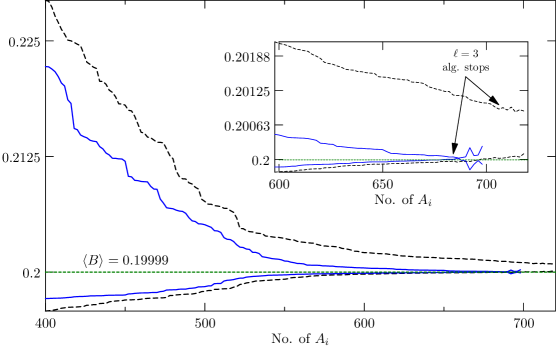
We used the following heuristics to decide when to stop adding more $A_{i}$’s and read the final result. First, at every step, we calculated the difference between the upperbound and the lowerbound to $\langle B\rangle$, and this served as a natural error scale. If the difference became negative (i.e., lowerbound was greater than the upperbound), we took the results of the previous step. Additionally, we stopped if the graph started to “wiggle”: if at one step the upperbound or lowerbound were worsened with respect to the previous step by more than 1% of the error length scale, we stopped and used the result of the previous step. In all runs (in systems B,C,D) this procedure resulted in an SDP estimate that is based on about 520-710 $A_{i}$ matrices.

A typical evolution of the upper/lower bounds for $\ell=3,4$ as the number of $A_{i}$ increases is presented in Fig. 4. The graph shows the evolution of the bounds in the case of system D (the XY model with random transverse field) with the random projector.

The full numerical results for the four systems are summarized in Tables 1,2,3,4. Table 1 presents the $\ell=3,4$ basic algorithm results for system A, the frustration-free AKLT model. The other three tables are for the frustrated models B,C,D, and they also include the CGO results. For each test we present the lowerbound and the upperbound in the form of a $[k_{min},k_{max}]$ range, as well as the estimated error $\Delta:=\frac{1}{2}(k_{max}-k_{min})$.

In the frustrated case, the $\ell=3,4$ radii of the local environment are well below the range where decay of correlation should be felt. It is not surprising then that the basic algorithm in these cases performs very badly, and is unable to give a single meaningful digit in the approximation of $\langle B\rangle$. At the same time, quite remarkably, the CGO algorithm manages to recover 3–4 digits (and often 4–5 digits) from $\langle B\rangle$. Moreover, these results are always better than their equivalent basic results for the frustration-free AKLT model, despite having a much larger correlation length ($\xi=8.8$ and $\xi=4.3$ vs. $\xi=0.9$ for the AKLT) and a much larger $V_{L}$ subspace ($q=36$ vs. $q=4$ for the AKLT).

VI Conclusions

We have presented a new approach to approximate the expectation value of a local operator given a PEPS tensor-network. Our initial observation is that while this is generally a computationally hard task (#P-hard), it is not necessarily the case for PEPS that represent gapped ground states, since these states have much more structure. Our approach circumvents the exponentially expensive contraction of the environment by estimating the local expectation value using only a local patch of the PEPS tensor-network around it. We have presented two algorithms to accomplish that. The basic algorithm simply diagonalizes the observable in the subspace $V_{L}$ and uses its extreme eigenvalues as upper/lower bounds for the expectation value. We have argued that this range is expected to converge as the radius of the local patch increases; it should in particular be useful for frustration-free systems. The second algorithm, CGO, builds upon the basic algorithm, but uses optimization over commutators to narrow down the eigenvalue range significantly. For it to work, the system has to be frustrated.

As demonstrated by our numerical tests, both algorithms allow one to extract a significant amount of information about the local expectation value using only a local patch of the surrounding tensor network. Contrary to what one might have expected, it seems that in frustrated systems much more information can be extracted from a local patch. In hindsight, this is reasonable: in frustrated systems the ground state is not a common eigenstate of all local terms ; only once we consider all local terms, we satisfy the eigenstate equation. This implies that the action of one local term must somehow cancel the action of other local terms, and this inter-dependence leads to many non-trivial constraints that can be exploited to recover $\rho_{L}$ from its underlying subspace (see Corollary 3).

Our work leaves many open questions for future research. From a numerical point of view, the most immediate question we would like to answer is how effective the CGO algorithm is in 2D. As it stands now, repeating the same procedure that we have used in the 1D case is impractical. Tentatively, for the CGO algorithm to work, one needs a high enough $D$ that would yield good approximation to the groundstate of a frustrated system, and in addition the dimension of the $V_{L}$ subspace should be smaller than the physical dimension of the spins inside $L$ – i.e., the area law should be non-trivially felt. Consider, for example, the rectangular grid in Fig. 1. There, we have $\dim V_{L}=D^{2(4\ell+3)}$ while the physical dimension goes like $d^{2(\ell+1)^{2}}$. So if we consider a $D=4$ PEPS over $d=2$ spins, the physical dimension wins over $\dim V_{L}$ at $\ell=7$, and reasonable results are expected at $\ell=8$ or beyond. This would mean one has to work with matrices of size $2^{162}\times 2^{162}$, an impossible task. It is therefore clear that the CGO algorithm cannot be used directly in 2D. Nevertheless, it might still be possible to apply it in approximate manner. For example, by projecting the system to a random subspace and using concentration results like the Johnson-Lindenstrauss lemma Johnson and Lindenstrauss (1984), or perhaps, by exploiting the symmetries in the problem (like translation invariance) in a clever way.

It would be also interesting to see if some aspects of CGO can be used in existing PEPS algorithms. The constraints of Corollary 3 may be useful in improving the simple-update method; even if we deal with small regions $L$ that do not provide a unique answer for $\rho_{L}$, satisfying the constraints in Corollary 3 may improve upon the simple product-state approximation of the environment. In addition, they might be useful for increasing the numerical stability of current algorithms. Finally, from a numerical point of view it would be interesting to see if Corollary 3 could be used to verify that we have an eigenstate at our hands. This might be useful, for example, for settling the nature of the groundstate of the antiferromagnetic Heisenberg model on the kagome lattice Evenbly and Vidal (2010); Yan et al. (2011); Depenbrock et al. (2012); Iqbal et al. (2013); Capponi et al. (2013).

From a more theoretical point of view, it would be interesting to gain better understanding of the CGO algorithm, and in particular the implications of the constraints in Corollary 3. For example, can we find sufficient conditions to when the algorithm gives good approximations (i.e., narrow $[k_{min},k_{max}]$ range)? From a computational complexity point of view, this might be a step in showing that PEPS of ground states can serve as an NP witness. A much more ambitious goal in that direction would be to show that the complexity of the local Hamiltonian problem for gapped Hamiltonians on a regular lattice with a unique ground state is inside NP.

Appendix A Proof of Lemma 2

The proof of Lemma 2 utilizes the detectability-lemma Aharonov et al. (2011) (see also LABEL:ref:AAV2016-DLD), and to a large extent already appeared in LABEL:ref:AAVZ2011-DL. We give the full proof here for sake of completeness.

We start by introducing the detectability lemma. Given a local Hamiltonian $H=\sum_{i}h_{i}$, we define for every $h_{i}$ a projector $P_{i}$ that projects onto its local ground space. Next we partition the $P_{i}$ terms into $g$ ‘layers’, such that each layer is a collection of projectors with disjoint support. For example, a 1D chain can be partitioned into two layers – one for projectors on $(i,i+1)$ with even $i$’s, and the second for odd $i$’s. Then for every layer $\ell$, we define the projector $\Pi_{\ell}$, which is the product of all the $P_{i}$ projectors in that layer; it is the projector onto the common ground space of all local terms in that layer. The detectability lemma operator, $\mathop{\rm DL}\nolimits(H)$ is then defined to be the product of the layer projectors: $\mathop{\rm DL}\nolimits(H):=\Pi_{1}\cdots\Pi_{g}$. Because the system is frustration free, it follows that $\mathop{\rm DL}\nolimits(H)|\Omega\rangle=|\Omega\rangle$. The detectability lemma states that if both the number of layers and the spectral gap of $H$ are of $\mathcal{O}(1)$, then for every state $|\psi\rangle$ orthogonal to the ground space, $\|\mathop{\rm DL}\nolimits(H)|\Omega^{\perp}\rangle\|^{2}\leq c<1$ for some constant $c$. Therefore, taking $\ell$ powers of the detectability lemma operator, we get an exponentially good approximation to the ground space projector:

$$\|\mathop{\rm DL}\nolimits^{\ell}(H)-|\Omega\rangle\langle\Omega|\|\leq e^{-\mathcal{O}(\ell)}\,.$$ (26)

Let us now return to the proof of the lemma. It consists of two steps. The first step is to notice that

$$B_{L}|\Omega\rangle=P_{V}B|\Omega\rangle=P_{V}\mathop{\rm DL}\nolimits^{\ell^{\prime}}(H)B|\Omega\rangle\,,$$ (27)

where $\ell^{\prime}=\mathcal{O}(\ell)$. The first equality follows from definition. The second equality follows from writing $\mathop{\rm DL}\nolimits(H)^{\ell^{\prime}}$ in terms of the local $P_{i}$ projectors, and noticing that each such $P_{i}$ projector can be either ‘pulled’ from the $P_{V}$ projector or from the ground state $|\Omega\rangle$. This is illustrated in Fig. 5 for the 1D case, see LABEL:ref:AAVZ2011-DL for more details.

Figure 5: Illustration of the second inequality in Eq. (27) in the 1D case. The ovals represent the $P_{i}$ projectors in $\mathop{\rm DL}\nolimits^{\ell^{\prime}}(H)$, organized in layers. The dark gray ovals are projectors that can be ‘pulled’ out from the $P_{V}$ operator (here, on the bottom). They form a sort of casual ‘light-cone’ defined by the local operator $B$. The rest of the projectors (represented by light-gray ovals) can be pulled out of the ground state $|\Omega\rangle$ (here, at the top).

The second step uses (26) to replace $\mathop{\rm DL}\nolimits^{\ell^{\prime}}(H)$ by $|\Omega\rangle\langle\Omega|+e^{-\mathcal{O}(\ell^{\prime})}=|\Omega\rangle\langle\Omega|+e^{-\mathcal{O}(\ell)}$, giving us

$$B_{L}|\Omega\rangle =P_{V}\cdot|\Omega\rangle\langle\Omega|\cdot B|\Omega\rangle+e^{-\mathcal{O}(\ell)}$$ (28)

$$=\langle B\rangle|\Omega\rangle+e^{-\mathcal{O}(\ell)}\,.$$

This proves the lemma.

References

- Orús (2014) R. Orús, Annals of Physics 349, 117 (2014).
- White (1992) S. R. White, Phys. Rev. Lett. 69, 2863 (1992).
- White (1993) S. R. White, Phys. Rev. B 48, 10345 (1993).
- Östlund and Rommer (1995) S. Östlund and S. Rommer, Physical review letters 75, 3537 (1995).
- Rommer and Östlund (1997) S. Rommer and S. Östlund, Physical Review B 55, 2164 (1997).
- Verstraete and Cirac (2004) F. Verstraete and J. I. Cirac, eprint arXiv:cond-mat/0407066 (2004), cond-mat/0407066 .
- Verstraete et al. (2008) F. Verstraete, V. Murg, and J. I. Cirac, Advances in Physics 57, 143 (2008), arXiv:0907.2796 .
- Sierra and Martin-Delgado (1998) G. Sierra and M. A. Martin-Delgado, arXiv preprint cond-mat/9811170 (1998), arXiv:cond-mat/9811170 .
- Hieida et al. (1999) Y. Hieida, K. Okunishi, and Y. Akutsu, New Journal of Physics 1, 7 (1999), arXiv:cond-mat/9901155 .
- Nishino et al. (2001) T. Nishino, Y. Hieida, K. Okunishi, N. Maeshima, Y. Akutsu, and A. Gendiar, Progress of Theoretical Physics 105, 409 (2001), arXiv:cond-mat/0011103 .
- Shi et al. (2006) Y.-Y. Shi, L.-M. Duan, and G. Vidal, Phys. Rev. A 74, 022320 (2006).
- Vidal (2008) G. Vidal, Phys. Rev. Lett. 101, 110501 (2008).
- Schuch et al. (2008) N. Schuch, M. M. Wolf, F. Verstraete, and J. I. Cirac, Phys. Rev. Lett. 100, 040501 (2008).
- Xie et al. (2014) Z. Y. Xie, J. Chen, J. F. Yu, X. Kong, B. Normand, and T. Xiang, Phys. Rev. X 4, 011025 (2014).
- Schuch et al. (2007) N. Schuch, M. M. Wolf, F. Verstraete, and J. I. Cirac, Phys. Rev. Lett. 98, 140506 (2007).
- Nishino and Okunishi (1996) T. Nishino and K. Okunishi, Journal of the Physical Society of Japan 65, 891 (1996), arXiv:cond-mat/9507087 .
- Orús and Vidal (2009) R. Orús and G. Vidal, Phys. Rev. B 80, 094403 (2009), arXiv:0905.3225 .
- Orús (2012) R. Orús, Phys. Rev. B 85, 205117 (2012), arXiv:1112.4101 .
- Vanderstraeten et al. (2015) L. Vanderstraeten, M. Mariën, F. Verstraete, and J. Haegeman, Phys. Rev. B 92, 201111 (2015), arXiv:1507.02151 .
- Levin and Nave (2007) M. Levin and C. P. Nave, Phys. Rev. Lett. 99, 120601 (2007), arXiv:cond-mat/0611687 .
- Xie et al. (2009) Z. Y. Xie, H. C. Jiang, Q. N. Chen, Z. Y. Weng, and T. Xiang, Phys. Rev. Lett. 103, 160601 (2009), arXiv:0809.0182 .
- Zhao et al. (2010) H. H. Zhao, Z. Y. Xie, Q. N. Chen, Z. C. Wei, J. W. Cai, and T. Xiang, Phys. Rev. B 81, 174411 (2010), arXiv:1002.1405 .
- Xie et al. (2012) Z. Y. Xie, J. Chen, M. P. Qin, J. W. Zhu, L. P. Yang, and T. Xiang, Phys. Rev. B 86, 045139 (2012), arXiv:1201.1144 .
- Pižorn et al. (2011) I. Pižorn, L. Wang, and F. Verstraete, Phys. Rev. A 83, 052321 (2011), arXiv:1103.2343 .
- Lubasch et al. (2014a) M. Lubasch, J. I. Cirac, and M.-C. Bañuls, Phys. Rev. B 90, 064425 (2014a), arXiv:1405.3259 .
- Jiang et al. (2008) H. C. Jiang, Z. Y. Weng, and T. Xiang, Phys. Rev. Lett. 101, 090603 (2008), arXiv:0806.3719 .
- Lubasch et al. (2014b) M. Lubasch, J. I. Cirac, and M.-C. Bañuls, New Journal of Physics 16, 033014 (2014b), arXiv:1311.6696 .
- Hastings (2004) M. B. Hastings, Phys. Rev. B 69, 104431 (2004), arXiv:cond-mat/0305505 .
- Hastings and Koma (2006) M. B. Hastings and T. Koma, Communications in Mathematical Physics 265, 781 (2006), arXiv:math-ph/0507008 .
- Nachtergaele and Sims (2006) B. Nachtergaele and R. Sims, Communications in Mathematical Physics 265, 119 (2006), arXiv:math-ph/0506030 .
- Kuwahara et al. (2015) T. Kuwahara, I. Arad, L. Amico, and V. Vedral, arXiv preprint arXiv:1502.05330 (2015), arXiv:1502.05330 .
- Perez-Garcia et al. (2008) D. Perez-Garcia, F. Verstraete, M. M. Wolf, and J. I. Cirac, Quantum Info. Comput. 8, 650 (2008), arXiv:0707.2260 .
- Michalakis and Zwolak (2013) S. Michalakis and J. P. Zwolak, Communications in Mathematical Physics 322, 277 (2013), arXiv:1109.1588 .
- Cirac et al. (2013) J. I. Cirac, S. Michalakis, D. Pérez-García, and N. Schuch, Phys. Rev. B 88, 115108 (2013).
- Hastings (2006) M. B. Hastings, Phys. Rev. B 73, 085115 (2006), arXiv:cond-mat/0508554 .
- Affleck et al. (1987) I. Affleck, T. Kennedy, E. H. Lieb, and H. Tasaki, Phys. Rev. Lett. 59, 799 (1987).
- Affleck et al. (1988) I. Affleck, T. Kennedy, E. H. Lieb, and H. Tasaki, Comm. Math. Phys. 115, 477 (1988).
- Knabe (1988) S. Knabe, Journal of Statistical Physics 52, 627 (1988).
- Yamashita et al. (2012) M. Yamashita, K. Fujisawa, M. Fukuda, K. Kobayashi, K. Nakta, and M. Nakata, in In Handbook on Semidefinite, Cone and Polynomial Optimization: Theory, Algorithms, Software and Applications, edited by M. F. Anjos and J. B. Lasserre (Springer, NY, USA, 2012) Chap. 24, pp. 687–714.
- Yamashita et al. (2010) M. Yamashita, K. Fujisawa, K. Nakata, M. Nakata, M. Fukuda, K. Kobayashi, and K. Goto, A high-performance software package for semidefinite programs: SDPA 7, Tech. Rep. B-460 (Dept. of Mathematical and Computing Science, Tokyo Institute of Technology, Tokyo, Japan, 2010) http://sdpa.sourceforge.net/index.html.
- Note (1) Strictly speaking, one can have a frustrated system in which the groundstate is a common eigenstate – for example, a frustrated classical system. However, in some sense these are not ‘genuine’ frustrated systems, since they can be trivially transformed into a frustration-free system by by locally subtracting an identity term from every local term in the Hamiltonian. This would make the system frustration-free and only shift its spectrum by a constant.
- Johnson and Lindenstrauss (1984) W. B. Johnson and J. Lindenstrauss, Contemporary mathematics 26, 1 (1984).
- Evenbly and Vidal (2010) G. Evenbly and G. Vidal, Phys. Rev. Lett. 104, 187203 (2010), arXiv:0904.3383 .
- Yan et al. (2011) S. Yan, D. A. Huse, and S. R. White, Science 332, 1173 (2011), arXiv:1011.6114 .
- Depenbrock et al. (2012) S. Depenbrock, I. P. McCulloch, and U. Schollwöck, Phys. Rev. Lett. 109, 067201 (2012), arXiv:1205.4858 .
- Iqbal et al. (2013) Y. Iqbal, F. Becca, S. Sorella, and D. Poilblanc, Phys. Rev. B 87, 060405 (2013), arXiv:1209.1858 .
- Capponi et al. (2013) S. Capponi, V. R. Chandra, A. Auerbach, and M. Weinstein, Phys. Rev. B 87, 161118 (2013), arXiv:1210.5519 .
- Aharonov et al. (2011) D. Aharonov, I. Arad, U. Vazirani, and Z. Landau, New Journal of Physics 13, 113043 (2011), arXiv:1011.3445 .
- Anshu et al. (2016) A. Anshu, I. Arad, and T. Vidick, ArXiv e-prints (2016), arXiv:arXiv:1602.01210 [quant-ph] .