Gravitational acceleration and edge effects in molecular clouds

Gravity plays important roles in the evolution of molecular clouds. We present an acceleration mapping method to estimate the acceleration induced by gravitational interactions in molecular clouds based on observational data. We find that the geometry of a region has a significant impact on the behavior of gravity. In the Pipe nebula which can be approximated as a gas filament, we find that gravitational acceleration can effectively compress the end of this filament, which may have triggered star formation. We identify this as the “gravitational focusing” effect proposed by Burkert & Hartman (2004). In the sheet-like IC348-B3 region, gravity can lead to collapse at its edge, while in the centrally condensed NGC1333 cluster-forming region gravity can drive accretion towards the center. In general, gravitational acceleration tends to be enhanced in the localized regions around the ends of the filaments and the edges of sheet-like structures. Neglecting magnetic fields, these “gravitational focusing” and “edge collapse” effects can promote the formation of dense gas in a timescale that is much shorter than the global dynamical time. Since the interstellar medium is in general structured, these edge effects should be prevalent.

1 Introduction

Star formation takes place in the dense and shielded parts of the molecular interstellar medium (ISM) (Dobbs et al., 2014), and it is probably determined by a combination of turbulence (Mac Low & Klessen, 2004; Hennebelle & Falgarone, 2012), gravity (Heyer et al., 2009; Ballesteros-Paredes et al., 2011, 2012), magnetic field (Li et al., 2014) and ionization radiation (Whitworth et al., 1994; Dale et al., 2009).

Gravity is one of the fundamental forces in nature, and it plays a determining role in the formation of the stars. However, observational understandings of its importance are still limited. Various methods have been proposed to quantify the importance of gravity on local (Bertoldi & McKee, 1992) and global (Li et al., 2015a) as well as various immediate scales (Rosolowsky et al., 2008; Goodman et al., 2009). In most of these methods, the effect gravity is estimated from the bulk properties of the regions obtained through averaging (e.g. the total mass and bulk velocity dispersion). In contrast to these, we propose a new method to study how gravity acts on individual structures.

It is expected that detailed morphologies of the gas are tightly linked to the star formation activities. This can be illustrated by the simulations of Burkert & Hartmann (2004); Hartmann & Burkert (2007). In a simplified case, the collapse of a roundish disk of a constant surface density under the influence of self-gravity is simulated. Different from the common perception that the disk will merely shrink in radius, the simulation shows that matter accumulates at its edge. Such an accumulation of gas leads to subsequent formation of filaments at the edge and finally dense cores. The collapse of filaments are also simulated (see also Clarke & Whitworth, 2015; Seifried & Walch, 2015), and it is found that matter accumulates at the ends of the filaments. To understand these phenomena, one needs to understand how gravity acts on gas in regions with different geometries. These information can not be obtained through e.g. the virial parameter. A better method which can provide estimates on the importance of gravity in regions with arbitrary geometries is thus needed.

There have been growing interests in studying filamentary structures in molecular clouds (André et al., 2010; Arzoumanian et al., 2011; Peretto et al., 2012, 2014; Palmeirim et al., 2013; Könyves et al., 2010; Schneider et al., 2012; André et al., 2014). Both numerical and analytical approaches have been employed to understand the evolution of these structures (Toalá et al., 2012; Tomisaka, 1995) (Smith et al., 2014b; Seifried & Walch, 2015; Clarke & Whitworth, 2015) (Heitsch & Hartmann, 2014; Toci & Galli, 2015; Inutsuka & Miyama, 1992; Wang et al., 2015). Filamentary structures have also been identified at $10^{2}-10^{3}\;\rm pc$ scale (Li et al., 2013; Ragan et al., 2014; Smith et al., 2014a; Goodman et al., 2014; Wang et al., 2015). Due to their highly irregular morphologies, we expect gravity to behave in a non-uniform way in these regions.

In this paper, we introduce an acceleration mapping method to quantify the effect of gravity on molecular ISM. Our general aim is to provide intuitive and qualitative pictures of the strength of gravitational acceleration in molecular clouds. Section 2 we introduce the method. The effect of gravity in accelerating gas is discussed in Sec. 3. Then we apply it to idealized examples as well as real observational data (Sections 4, 5). The importance of gravitational acceleration in star formation is discussed in detail in Sec. 6. In Section 7 we conclude.

2 Calculating acceleration

2.1 General concept

Observationally, gas is observed on the sky plane, and the distribution of gas along the line of sight is not easily observed. To compute gravitational potential, we assume that all the observed matter is distributed in a thin plate of thickness $H$. We make this assumption mainly because of observational limit, namely that matter can only be reliably mapped on the sky plane in most observations. A generalization of the method to the 3D case is straightforward.

In our work, we first compute gravitational potential based on a column density distribution. Then we compute gravitational acceleration distribution based on the gravitational potential. Finally, we combined the gravitational acceleration map with the column density map, and study the effect of gravity on matter. This is illustrated in Fig. 1.

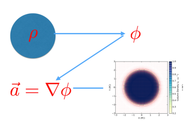
Figure 1: A illustration of our concept. See Sec. 2.1 for details. $\rho$ stands for density, $\phi$ stands for gravitational potential, and $\@vec{a}$ stands for acceleration.

2.2 Numerical realization

Observationally, matter can be observed on the sky plane as $\Sigma(x,y)$ where $\Sigma$ is the surface density. In our study, we compute gravitational acceleration based on $\Sigma(x,y)$.

Assuming the observed gas is distributed on the 2D sky plane with a thickness $H$, the projected gravitational potential can be computed as (Gong & Ostriker, 2011)

$$\Phi_{\@vec{k},\rm 2D}=\frac{-2\pi\;G\;\Sigma_{\@vec{k,\rm 2D}}}{|\@vec{k}|(1+|\@vec{k}H|)}\;,$$ (1)

where $\Phi_{\@vec{k},\rm 2D}$ is the projected gravitational potential in the $\@vec{k}$ space, and $\Sigma_{\@vec{k},\rm 2D}$ is the surface density in the $\@vec{k}$ space. Numerically, we first make a Fourier transform to $\Sigma(x,y)$ and obtain $\Sigma_{\@vec{k}}$, then use Eq. 1 to evaluate $\Phi_{\@vec{k},\rm 2D}$. Finally, $\Phi(x,y)$ is obtained through an inverse Fourier transform of $\Phi_{\@vec{k},\rm 2D}$.

In reality, gravitational potential is a quantity defined in the 3D space. In this formalism, at one position on the sky plane $(x_{0},y_{0})$, the 2D projected gravitational potential $\Phi(x_{0},y_{0})$ is defined as $\Phi(x_{0},y_{0})=\Phi(x_{0},y_{0},z)$ where $z$ represent the direction of the line of sight and $z=0$ .

With the gravitational potential, acceleration can be derived:

$$\@vec{a}=-\nabla\Phi\;.$$ (2)

The gradient is evaluated with np.gradient from the numpy package.

The only parameter we need to introduce is the thickness along the $z$ direction $H$. In general, when $H$ is small, the structure of smaller scales are better represented, and when $H$ is large, small-scale structures tend to be smoothed out in the acceleration map. Ideally, $H$ should be chosen to be close to the real 3D thickness of the cloud. However, this is not feasible in practise. Here, we choose to use $H=0.3\;\rm pc$ throughout this paper. This is because observations have demonstrated that star formation tend to concentrate in clumps, whose sizes are close to parsec scale (Beuther et al., 2002; Molinari et al., 2000). The size of the clumps provides an hint to the expected thickness of the cloud. On the other hand, we do not choose a $H$ that is much larger than a parsec, because we would still like to study the small-scale structure of gravitational acceleration.

2.3 Boundary conditions

Computing gravitational potential and acceleration in the Fourier space automatically assumes periodic boundary condition. This means it is assumed that the input density distribution $\Sigma(x,y)$ repeats itself in the $x$–$y$ plane ( $\Sigma(x,y)=\Sigma(x+x_{0},y)=\Sigma(x,y+y_{0})=\Sigma(x+x_{0},y+x_{0})$ when the image have a size of (x0, y0)).

Since gravity is a long-range force, the presence of matter outside the box do have influences on the motion of gas inside the box. Therefore, the results are dependent on the boundary conditions which have to be specified.

In this work, for an input map of size $(x_{0},y_{0})$ we added zeros to the region where $x<0$, $x>x_{0}$, $y<0$ or $y>y_{0}$, and created a map of the size $(2\times x_{0},2\times y_{0})$. Then we use Eq. 1 to compute the gravitational potential. This is equivalent to assuming that the cloud is surrounded by a region devoid of matter. The size of the void region is comparable to the cloud size. One can also increase the size of this void region. Because gravitational force decays as $r^{-2}$, our results are not sensitive to this. However this will increase the computational cost significantly.

Nature is composed of a continuous distribution of matter, which are gravitationally interacting (e.g. molecular clouds are in constant gravitational interaction with the spiral arms). In computing our acceleration map, one has to isolate the object of interest and study the gravitational acceleration arising from the gravity originates for this object. This isolation procedure can also lead to inaccuracies. However, one can always evaluate these effects by comparing the expected gravitational acceleration from a body that is outside our box ($|\@vec{a}|\approx Gm/r^{2}$ where $m$ is the mass of the object outside our box, and $r$ its the distance from our object) with the acceleration computed in our map, to evaluate the effect of the simplified boundary conditions on our results.

2.4 Projection effects

The acceleration map we obtain with this method is computed at $z=0$. In reality matter are not distributed in a plane but are distributed in 3D. This will have an effect on our results. In general, acceleration maps are affected by projection effects, and cautions should always be taken when the region has a complicated structure or a multiple of velocity components. Here we briefly discuss various projection effects.

Because of line-of-sight contamination, physically unassociated structures can appear as coherent. This will certainly have an impact on our results. However, in many cases, the line-of-sight contamination can be accessed using 3D extinction (Sale et al., 2014) (Green et al., 2015; Chen et al., 2014; Kainulainen et al., 2014) (Hanson & Bailer-Jones, 2014; Berry & Ivezić, 2011; Lallement et al., 2014) or velocity information.

For clumpy structures, the fact that we can not distinguish structures along the line of sight only have a moderate influence on the results. Consider a portion of a clump that is separated from the center by a distance $L$. In our calculations, it is automatically assumed that the all the gas stays at $z=0$. If a portion of the cloud with mass $m$ stays at $z=z_{0}$ instead of $z=0$, the acceleration it contributes is $a\sim Gm/(L^{2}+z_{0}^{2})$. For a clump, because the geometry is close to symmetric, $z_{0}\lesssim L$, the error is relatively small, and is generally acceptable.

For filamentary structures, inclination has a significant impact on the result. To illustrate this one can look at the gravitational acceleration around a filament. Consider a filament of length $l_{0}$ and width $d$. The filament has a line mass of $\delta={\rm d}m/{\rm d}l$. The gravitational acceleration at one end of this filament can be solved approximately:

$$a=\int_{d}^{l_{0}}\frac{G\delta}{r^{2}}{\rm d}r=G\;\delta\;\Big{(}\frac{1}{d}-\frac{1}{l_{0}}\Big{)}\;,$$ (3)

where $G$ is the gravitational constant. Consider a case where the filament is not parallel to the sky plane but is inclined by an angle $\theta$. From the observer, $\delta^{\prime}=\delta/\cos(\theta)$, $d^{\prime}=d\,\cos(\theta)$ and $l^{\prime}=l_{0}\,\cos(\theta)$. Overall, according to Eq. 5, $a^{\prime}=a\,/\cos^{2}(\theta)$. If the filament is inclined by $45^{\circ}$, the gravitational acceleration will be over-estimated by a factor of $2$. A larger inclination leads to a larger error.

For sheet-like structures, inclination has some impacts on the results but these are in general acceptable. This can be illustrated by some examples in Burkert & Hartmann (2004) where the ellipse case shows a good similarity with the case of the roundish disk. Since we only expect our results to be accurate in the order-of-magnitude sense, the error arising from the inclination effect is in general acceptable.

To sum up, all the projection effects leads to some over-estimations of the acceleration. The line-of-sight contamination can be avoided in many cases using velocity information or extinction distance estimates. For clump-like structures, line-of-sight effects only moderately affect the computed acceleration structure. For filaments and sheets, a moderate inclination can often lead to a change in the estimated acceleration by a factor of 2, which is acceptable. The acceleration map computed in this work should thus capture the general behaviors of gravity in molecular clouds, but the values in the acceleration map is accurate only in the order-of-magnitude sense.

3 Acceleration and gas motion

Gravitation acceleration is important for the movement of gas. Consider that at $p_{1}$ the acceleration is $\@vec{a}_{1}$ and at $p_{2}$ the acceleration is $\@vec{a}_{2}$. Initially, both the gas at position $p_{1}$ an the gas at position $p_{2}$ have zero velocities. We are interested in the effect of acceleration in gas compression / dilation.

At time $t$, the different in separation is simply

$$\delta x=\frac{1}{2}|\@vec{a_{2}}-\@vec{a_{1}}|\times t^{2}\;.$$ (4)

What actually drives the gas compression, dilatation or shear is the (vector) difference in acceleration.

In a region, when the acceleration is larger, it is very likely that there exist significant contrasts in acceleration with respect to its surroundings. In this work, we choose to study the acceleration rather than the difference in acceleration for two reasons: First, in many cases, they are related. A large acceleration is usually related to a large acceleration difference. Second, there are other forces such as magnetic forces that are influencing the cloud evolution. To properly evaluate the impact of gravitational acceleration one need to compare the acceleration strength with e.g. pressure from the magnetic field. For this purpose, it is more practical to study acceleration instead of the difference in acceleration.

4 Applications to idealized examples

We apply the acceleration mapping method to several idealized examples. We consider acceleration from a thin disk, a filament and a centrally condensed gas clump.

4.1 Thin disk

In our thin disk example, we consider a disk of a radius of $1\;\rm pc$ and a surface density of $1\;\rm g\;\rm\;cm^{-2}$. The input is smoothed with a Gaussian kernel with $\sigma=2\rm\;pixels$, and we use $H=0.3\;\rm pc$ (see Eq. 1) throughout this paper. The results are presented in Fig. 2. In the disk case, the acceleration reaches a maximum at the edge of the disk. Under ideal situations, matter should accumulate at the regions where acceleration is enhanced, which was observed in Burkert & Hartmann (2004).

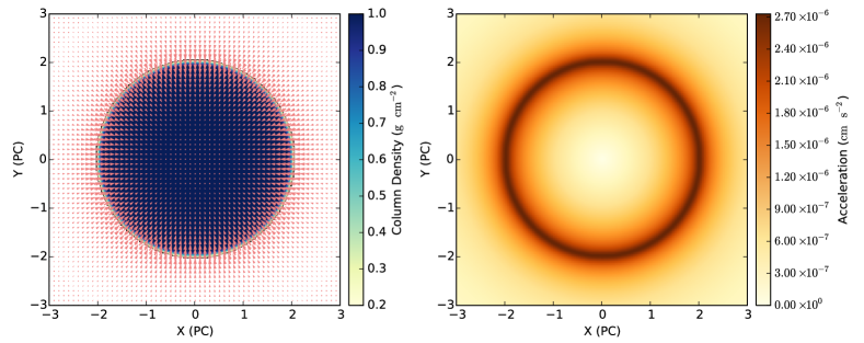
Figure 2: Left Panel: Density distribution and acceleration of our disk model with a radius of $1\;\rm pc$ and a surface density of $1\;\rm g\;\rm\;cm^{-2}$. The background image is the density distribution and the vectors stand for acceleration. Right Panel: A map of the magnitude of acceleration. A color-blindness-proof version of the this figure and be found in Appendix A.

4.2 Truncated filament

We consider a filament with a width of $0.1\;\rm pc$, a length of $1\;\rm pc$, and a peak surface density of $1\,\rm g\rm\;cm^{-2}$. Along the filament, the peak surface density is constant. Perpendicular to the filament, we assume a Plummer-like density profile:

$$\Sigma(r)=\Sigma_{\rm c}\frac{1}{1+(l/l_{\rm flat})^{{p}/2}}\;,$$ (5)

where $l$ is the projected distance to the ridge of the filament. We take $p=1.6$, $l_{\rm flat}=0.033\;\rm pc$ and $\Sigma_{\rm c}=1\rm\;g\;cm^{-2}$. Integrating over Eq. 5 gives a line mass of 1.27 $\;\rm g\,cm^{-2}\times pc$. The input is smoothed with a Gaussian kernel with $\sigma=2\rm\;pixels$. $H=0.3\rm\;pc$. The results have been shown in Fig. 3. The acceleration reaches its maximum at both ends of the filaments, and this should leads to collapse. This effect was observed in Burkert & Hartmann (2004) and was named “gravitational focusing” by the authors. Using Eq. 5 and set $d=l_{\rm flat}=0.033\;\rm pc$, $l_{0}=1\;\rm pc$ and $\delta=1.27\;\rm g\,cm^{-2}\times pc$ gives $a\approx 2\times 10^{-6}\;\rm cm\,s^{-2}$, in qualitative agreement with the results in Fig. 3.

Gravity is also responsible for driving accretion onto dense structures. Heitsch (2013) investigated the accretion onto dense filaments, and identified fan-like structures of gas velocities on filament ends. Such fan-like velocity structures resemble acceleration vectors in Fig. 3.

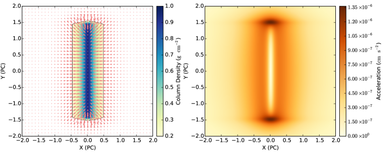
Figure 3: Left Panel: Density distribution and acceleration of our truncated filament model (see Section 4.2 for details). The background image is the density distribution and the vectors stand for acceleration. Right Panel: A map of the magnitude of acceleration. A color-blindness-proof version of the this figure and be found in Appendix A.

4.3 Centrally condensed clump

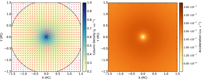
Figure 4: Left Panel: Density distribution and acceleration of our clump model (see Section 4.3 for details). The background image is the density distribution and the vectors stand for acceleration. Right Panel: A map of the magnitude of acceleration. A color-blindness-proof version of the this figure and be found in Appendix A.

We consider the effect of gravity on a centrally condensed structure which resembles those seen in observations (e.g. Kauffmann et al., 2010; Larson, 1981). We assume

$$\frac{\Sigma}{M_{\odot}\;\rm pc^{2}}=870\times\Big{(}\frac{r}{\rm pc}+0.1\Big{)}^{-0.7}\;,$$ (6)

where $\Sigma$ is the surface density and $r$ is the projected distance from the center. It mimic the structure of a gas condensation seen in observations. The gravitational acceleration structures are shown in Fig. 4. Here acceleration vectors converge to the center where the surface density reaches its maximum, and in this case, it will probably lead to a continuous accretion flow. The magnitudes of acceleration vectors are very small at the central region. This is because of symmetry, which leads the acceleration from the outer parts of the clump to cancels out.

5 Applications to observational data

After testing the method with the idealized cases, we apply the method to observational data.

5.1 Pipe Nebula

We obtain extinction maps from Rowles & Froebrich (2009); Froebrich & Rowles (2010). We use the 25 stars $A_{\rm v}$ maps which have a pixel size of 0.5 $\rm arcsec$. The extinction $A_{\rm v}$ and surface density are linked by (Bohlin et al., 1978)

$$\frac{n({\rm H_{2}})}{A_{\rm v}}=9.4\rm\times{10^{20}\;cm^{-2}\;mag^{-1}}\;.$$ (7)

The Pipe nebula locates at a distance of $\sim 160\;\rm pc$ (Alves & Franco, 2007; Knude & Hog, 1998). The cloud contains $\sim 10^{4}\;M_{\odot}$, and has an elongated morphology. It is believed that such a structure is shaped by the expansion of another Hii region (Gritschneder & Lin, 2012). Only $\sim 150\rm\;YSOs$ are found to be associated with the whole cloud (Kainulainen et al., 2009; Lombardi et al., 2006). Filamentary structures in the nebula have been found in recent Herschel observations (Peretto et al., 2012).

Star formation in the Pipe nebula is relatively quiescent, except the B59 region where a cluster of YSOs can be found (Brooke et al., 2007; Forbrich et al., 2010, 2009). The physical reason for this uneven distribution of star formation is still unclear. It is proposed that the star formation activity is triggered by compression from the nearby Sco OB2 association (Onishi et al., 1999; Peretto et al., 2012). Magnetic support might also play a role (Alves et al., 2008).

The Pipe nebula is an ideal target for our analysis, for two reasons. First, the region have a relatively high galactic latitude, which makes it relatively easy to separate it from the background. Second, the region has an elongated morphology, making it an ideal testbed for non-local effects of gravity.

In Fig. 5 we present surface density and acceleration structure of Pipe nebula. The extra acceleration on the lower left edge of the map is due to artifacts, since the nebula have a finite surface density inside the map, and outside the map it is assumed that the surface density is zero. Because sharp edges are introduced around the boundaries, artificial accelerations arise from the computations (see Sec. 2.3). Therefore these boundary regions are excluded from our analysis. The acceleration has been enhanced at region A (see Fig. 5) and the B59 region, and together with the “stem” region, these three form a system where region A and the B59 region are the ends of a truncated filament and the “stem” region correspond to the “body” of a filament, and accelerations are enhanced at the ends of this filament. The enhancement of acceleration at the ends results from the gravitational focusing effect observed in Burkert & Hartmann (2004) and in Section 4.2.

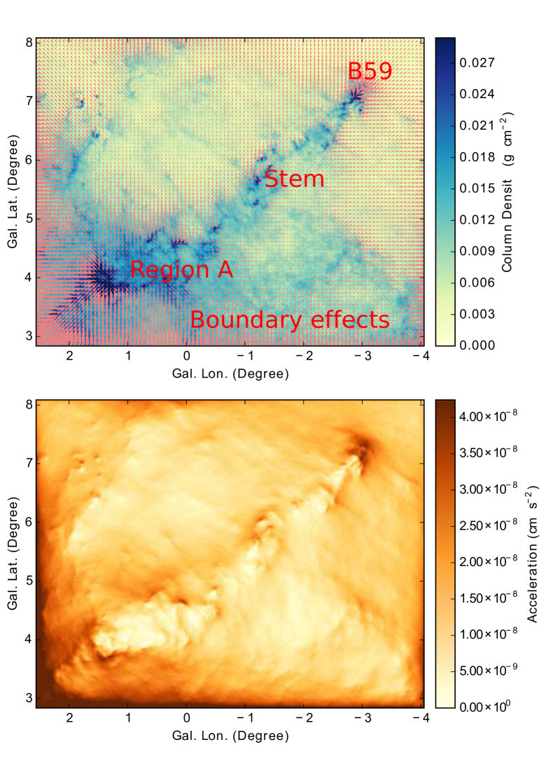
Figure 5: Upper Panel: surface density distribution and acceleration of the Pipe region. The background image is the surface density distribution and the vectors stand for acceleration. Lower Panel: A map of the magnitude of acceleration of the same region. The region A, “stem” region and B59 regions are indicated. Regions where the artifacts due to boundary effect are also indicated. Here one degree correspond to $\sim 3\;\rm pc$. A color-blindness-proof version of the this figure and be found in Appendix A.

In Fig. 6 we present surface density and acceleration structure of the stem and B59 region of the Pipe Nebula. YSO candidates from Forbrich et al. (2009) are overlaid. The B59 region shows up as a region where acceleration vector converges; this is also the region where the majority of the protostars are found. This implies a connection between gravitational acceleration and star formation.

The acceleration seen around the B59 region have two possible sources. The first and obvious source of acceleration is the gravity from the central part of the B59 where the surface density peaks. The second source of acceleration is the gravity contributed from the rest of the Pipe nebula. To further investigate the origin of acceleration we repeat the calculation by considering only the gas inside the B59 region, and compare the results with acceleration map computed for the whole Pipe nebula. The results are presented in Fig. 7. Several clear differences can be identified. First, acceleration computed for the B59 region alone converges to its center, and when the gravity of the whole Pipe nebula has been taken into account, acceleration only converges through the north-western part, and acceleration at the south-eastern part of the B59 region is suppressed. This difference is due to the contribution from gas the belongs to the Pipe nebula but outside the B59 region. Second, the magnitude of acceleration at the north-eastern part of the the B59 region is much higher when the gravity of the whole Pipe nebula have been taken into account, which indicates that gas from the whole Pipe nebula is contributing significantly to the gravitational acceleration observed in the B59 region. The large-scale acceleration can compress B59 region significantly.

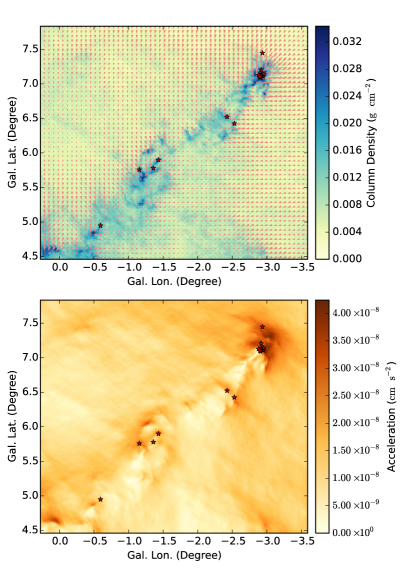
Figure 6: Upper Panel: surface density distribution and acceleration of the Pipe Nebula. The background image is the surface density distribution and the vectors stand for acceleration. Lower Panel: A map of the magnitude of acceleration of the same region. The red stars stand for the YSO candidates in (Forbrich et al., 2009). Here one degree correspond to $\sim 3\;\rm pc$. A color-blindness-proof version of the this figure and be found in Appendix A.

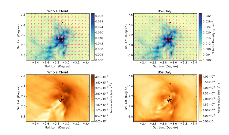
Figure 7: Upper Panels: surface density maps and acceleration of the B59 region in the Pipe Nebula. The background images are the surface density distribution and the vectors stand for acceleration. Lower Panels: Maps of the magnitude of acceleration of the same region. The red stars stand for the YSO candidates in Forbrich et al. (2009). The results shown in the left panels are computed by taking all the matter of the Pipe nebula into account (whole cloud), and the results shown in the right panels are computed by taking only the matter inside the B59 into account (B59 only). Here one degree correspond to $\sim 3\;\rm pc$. A color-blindness-proof version of the this figure and be found in Appendix A.

5.2 NGC1333 cluster-forming region

Centrally condensed gas clumps are common in star-forming regions. On such example is the cluster-forming region NGC1333 in the Perseus molecular cloud.

We obtain extinction map of the Perseus molecular cloud from the COMPLETE (Ridge et al., 2006) survey. First, we compute the gravitational acceleration for the whole region. Then we zoom into the NGC1333 region and study the structure. A distance of 250 pc is used in our calculations (Knude & Hog, 1998).

The results for the whole Perseus region is shown in Fig. 8, and the acceleration map exhibits a variety of behaviors in different regions.

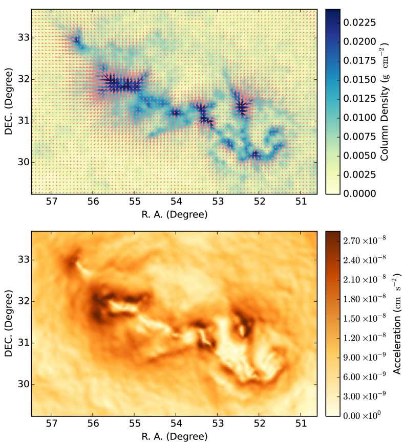
Figure 8: Upper Panel: surface density distribution and acceleration of the Perseus molecular cloud. The background image is the surface density distribution and the vectors stand for acceleration. Lower Panel: A map of the magnitude of acceleration of the same region. Here one degree correspond to $\sim 4.5\;\rm pc$. A color-blindness-proof version of the this figure and be found in Appendix A.

The results for NGC1333 are presented in Fig. 9. Here the acceleration has a relatively symmetric structure, and converges towards the center. This is mainly due to the mass concentration at the center of the region. In this case, gravity can potentially drive the accretion from the outskirts towards the center. This behavior is similar to what is found in Section 4.3 for the simplified centrally condensed clump model.

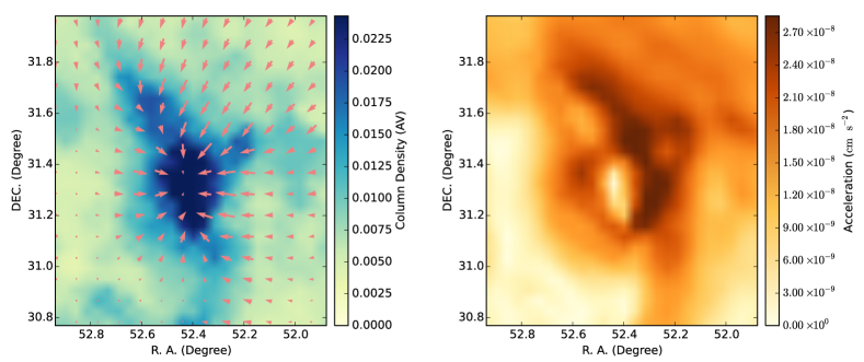
Figure 9: Left Panel: surface density distribution and acceleration of the NGC1333 region in the Perseus molecular cloud. The background image is the surface density distribution and the vectors stand for acceleration. Right Panel: A map of the magnitude of acceleration of the same region. Here one degree correspond to $\sim 4.5\;\rm pc$. A color-blindness-proof version of the this figure and be found in the Appendix A.

5.3 IC348-B3 star-forming region

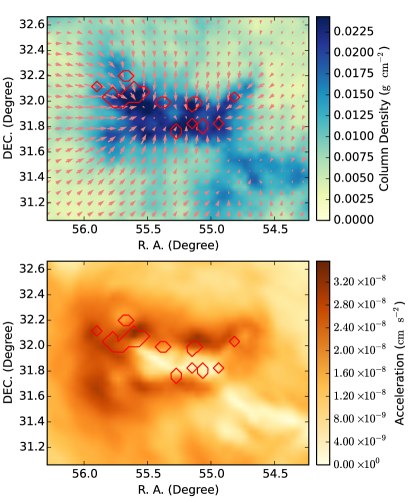
Figure 10: Upper Panel: surface density distribution and acceleration of the IC348-B3 region in the Perseus molecular cloud. The background image is the surface density distribution and the vectors stand for acceleration. Lower Panel: A map of the magnitude of acceleration of the same region. The red contours mark the region where starless and prestellar cores are found (Enoch et al., 2006). Here one degree correspond to $\sim 4.5\;\rm pc$. A color-blindness-proof version of the this figure and be found in Appendix A.

We consider acceleration in a highly irregular region – the IC348-B3 star-forming region in the Perseus molecular cloud. The region is considered to be more evolved (Gutermuth et al., 2009), and a young embedded cluster IC348 is found to be associated with the region.

In Fig. 10 we present the results. Positions of the dense cores are taken from Enoch et al. (2006), and they are marked with the red contours. Here acceleration concentrates at the edges of the cloud. The region where acceleration is enhanced coincide with the region where the dense cores are found. In this sense, the IC348 region resembles the case of the “Ghost” studied in Burkert & Hartmann (2004). This resemblance points to a picture where the star formation in the IC348 region traced by the dense cores are triggered because of the enhanced gravitational acceleration at the edges of the region.

In the inner part of the IC348-B3 region, albeit the presence of gas, the acceleration is reduced because of the apparent sheet-like geometry. This lack of acceleration should lead to a lack of the ability of the gas to collapse and hence a lack of star formation. Indeed, none of the dense cores in Enoch et al. (2006) are found at the inner part of the IC348-B3. This is similar to the thin disk example as discussed in Section 4.1.

6 Discussions

6.1 General importance

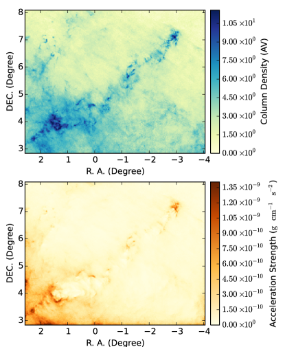
Figure 11: Upper Panel: A map of of surface density of the Pipe nebula. Lower Panel: A map of the magnitude of effective acceleration pressure $p_{\rm acceleration}\sim\Sigma\;|\@vec{a}|$. Here one degree correspond to $\sim 3.6\;\rm pc$.

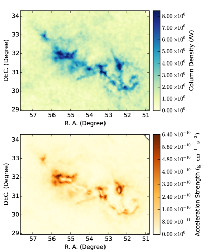
Figure 12: Upper Panel: A map of of surface density of the Perseus molecular cloud. Lower Panel: A map of the magnitude of effective acceleration pressure $p_{\rm acceleration}\sim\Sigma\;|\@vec{a}|$. Here one degree correspond to $\sim 4.5\;\rm pc$.

The acceleration map can be combined with the map of surface density to estimate the importance of gravity in accelerating the gas. This can be achieved by multiplying $|\@vec{a}|$ with the surface density map $\Sigma$. The effective acceleration pressure is

$$p_{\rm acceleration}=\frac{F_{\rm acceleration}}{S}=\frac{M\times|\@vec{a}_{\rm 3D}|}{S}\sim\Sigma\;|\@vec{a}_{\rm 2D}|\;,$$ (8)

where $\@vec{a}_{\rm 3D}$ is the 3D acceleration and $\@vec{a}_{\rm 2D}$ is the 2D projected acceleration. We assume that $|\@vec{a}_{\rm 3D}|\sim|\@vec{a}_{\rm 2D}|$.

Eq. 8 provides an order-of-magnitude estimate of the importance of acceleration in molecular clouds, and can be used to obtain maps of the importance of acceleration on the sky plane.

In the localized regions, the effective acceleration pressure can reach $p\sim 10^{-9}\rm g\;cm^{-1}\;s^{-2}$, which correspond to $\dot{p}/k_{\rm B}\sim 10^{7}\;\rm K\;cm^{-3}$ where $k_{\rm B}$ is the Boltzmann’s constant. This is much larger than the external ambient pressure of molecular clouds estimated in previous works (Heyer et al., 2009; Field et al., 2011) .

The comparison between the effective pressure and the ambient pressure provides estimates on the importance of gravitational acceleration. However, because our calculations are done in 2D rather than in 3D, the results needs to be interpreted with caution. The pressure is isotropic, and the momentum injection from acceleration is anisotropic. Consider a 3D cuboid of a size $(l_{x},l_{y},l_{z})$ where $z$ stand for the direction of the line of sight, and the acceleration points toward the $y$ direction. The momentum injection from gravitational acceleration is $\dot{P}_{\rm accel}\approx\rho a_{y}l_{x}l_{y}l_{z}\approx\Sigma a_{y}\times l_{x}l_{y}\approx p_{\rm accel}l_{x}l_{y}$ where $\Sigma$ is the surface density. The momentum injection from the ambient pressure along the $y$ direction is $\dot{P}_{\rm pressure}\approx p_{\rm ambient}l_{x}l_{z}$ where $p_{\rm ambient}$ is the ambient pressure. $\dot{P}_{\rm accel}/\dot{P}_{\rm pressure}\approx p_{\rm accel}/p_{\rm ambient}$ requires $l_{y}\approx l_{z}$. In other words, the ratio between $p_{\rm accel}$ and $p_{\rm ambient}$ is a meaningful representation of the relative importance between acceleration and ambient pressure only when the region is only moderately extended along the line of sight. When the region is highly elongated along the line of sight, the importance of the effective acceleration pressure will be over-estimated.

In our acceleration map, $p_{\rm accel}$ can be $100$ times stronger than the local ambient pressure. External pressure can be important of the cloud as a whole, but gravitational acceleration will be extremely effective in the localized regions.

We also derive the timescale on which gravitational acceleration can change the concentration of the gas significantly. Observationally, it is found that dense gas concentrate in clumps and filaments, and the clumps are typically $\sim 1\rm pc$ large (Molinari et al., 2000; Beuther et al., 2002). For acceleration to create such gas clumps, we have ( using $l=1/2\;a\;t^{2}$ where $l$ is the size of the clump, $a$ is the acceleration and $t$ is the time)

$$t_{\rm clump}\approx\sqrt{\frac{l}{a}}\;,$$ (9)

For the Pipe nebula, $a\sim 10^{-8}\;\rm cm\,s^{-2}$, from which we estiamte a timescale of $t_{\rm clump}\sim 10^{6}\;\rm yr$. $t_{\rm clump}$ is about one order of magnitude shorter than typical cloud lifetimes, which are $\sim 10^{7}\;\rm yr$ (Williams & McKee, 1997; Blitz et al., 2007), and is much shorter than the global dynamical timescale of the Pipe nebula, which is around $t_{\rm dyn}\sim\sqrt{r^{3}/Gm}\sim\,3\times 10^{7}\rm yr$ where r is the size of the cloud. We used $L=15\;\rm pc$ and $m=10^{4}M_{\odot}$ . Neglecting other factors such as magnetic fields, gravitational acceleration can potentially trigger fast collapses in the localized regions.

6.2 Diverse behaviors

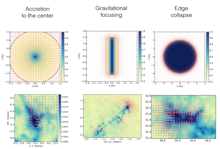
Figure 13: A summary of the effects discussed in this work. The first row lists the names of the effects, the second row shows the idealized models, and the third row shows the relevant observations. The first model on the second row is discussed in Section 4.3, the second model on the second row is discussed in Section 4.2, and the third model on the second row is discussed in 4.1. The first observation on the third row is the NGC1333 region (Sec. 5.2), the second observation is the Pipe nebula (Sec. 5.1), and the third observation is the IC348-B3 region (Sec. 5.3).

We find that gravitational acceleration exhibits diverse behaviors in various regions, which can be summarized in Fig. 13.

In the Pipe nebula, we find that acceleration concentrates at the B59 region. The acceleration structure of the Pipe nebula can be explained by the “gravitational focusing” effect proposed by Burkert & Hartmann (2004). Similar phenomena are seen in many of the recently-observed filaments (Li et al., 2015b; Kainulainen et al., 2015; Beuther et al., 2015; Wang et al., 2014),

We also the method to the Perseus molecular cloud, and find that in the IC348-B3 region both the acceleration and the formation of dense gas tend to occur at the edges of the region, and this is consistent with the “edge collapse” in Burkert & Hartmann (2004). Acceleration in the NGC1333 cluster-forming region converges towards the center, indicating that gravity can collect matter towards the center of the region and feed star formation. In sum, we that gravitational acceleration plays important roles at least in the following ways:

1. In driving the accretion onto the central parts of centrally-condense regions (accretion).

2. In driving the collapse at the ends of the filamentary structures (gravitational focusing).

3. In driving the collapse at edges of flat structures (edge collapse).

The various ways in which gravitational acceleration functions are summarized in Fig. 13. It should be noted that in many cases these different mechanisms occur simultaneously. One example is the gas accretion at the ends of a filament. In this case, gravitational focusing is responsible for the collapse of the filament ends, and if a diffuse envelope exists around the filament, accretion will occur which brings gas from the diffuse phase to the ends of the filament (Heitsch, 2013).

7 Conclusions & Discussions

In this work, we present a gravitational acceleration mapping method to quantify the importance of gravity in molecular clouds, and study the impact of gravitational acceleration on the evolution of molecular clouds.

The method takes observational maps of surface density distributions on the sky plane as the inputs, and provides maps of the gravitational acceleration on the sky plane. It provides a qualitative and intuitive picture of gravity in molecular clouds. We apply our method to both simplified models and observations including Pipe nebula and the Perseus molecular cloud.

With observational data, we find that the star formation activities in the IC-348 region traced by dense cores can be explained by edge collapse, and the concentration of star formation in the B59 region of the Pipe nebula is consistent with a picture where gravitational focusing contributes to the compression of the gas. In the NGC1333 cluster-forming region, acceleration can drive accretion from the outskirts to the center. The main observational results are summarized as follows:

• Gravitational acceleration exhibits diverse behaviors in various regions.

• Gravitational acceleration tends to concentrate in the localized regions in molecular clouds.

• In the localized regions, the strength of the acceleration exceeds by much the mean external pressure of molecular clouds.

• In the localized regions, the concentration of acceleration can lead to local collapse. The local collapse can occur in a timescale that is much shorter (e.g. $10^{6}$ yr) than the dynamical timescale of the cloud.

However, a complete picture of gas evolution is yet to be achieved since we need to fully understand the interplay between magnetic field, turbulence and gravity in these these regions. There are ample observational evidences that magnetic fields are important in star-forming regions (Li et al., 2014). Remarkably-ordered magnetic fields have been revealed in several star-forming regions (Qiu et al., 2014; Zhang et al., 2014; Alves et al., 2008; Chapman et al., 2011; Planck Collaboration et al., 2015; Li et al., 2015b). Magnetic fields are observed to be either parallel or perpendicular to filamentary structures (Zhang et al., 2014; Planck Collaboration et al., 2015). Magnetic field strength can also vary strongly within different star-forming regions (e.g. Alves et al., 2008). Strong magnetic field can affect fragmentation significantly (Seifried & Walch, 2015). The effect of turbulence is not considered explicitly in this formalism. It is possible that in regions such as B59, turbulent motion can be driven as a result of the enhanced acceleration (Klessen & Hennebelle, 2010). These possibilities should be investigated in subsequent works.

The Milky Way ISM is in general structured. We expect that the non-local effect of gravity to be important in the majorities of the cases. The acceleration mapping method presented in this paper provides a detailed and intuitive picture of gravity in the molecular ISM. The results can be combined with studies of turbulent motions and magnetic field observations to finally achieve a clear picture of star formation.

Appendix A Colorblindness-proof version of some of the figures

In this section we provide plots that are suitable for those with color-blindness. Fig. 14 correspond to Fig. 2.

Figure 14: Left Panel: Density distribution and acceleration for our disk model with a radius of $1\;\rm pc$ and a surface density of $1\;\rm g\;\rm\;cm^{-2}$. The background image is the density distribution and the vectors stand for acceleration. Right Panel: A map of the magnitude of acceleration.

Fig. 15 correspond to Fig. 3.

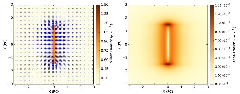
Figure 15: Left Panel: Density distribution and acceleration for our truncated filament model (see Section 4.2 for details). The background image is the density distribution and the vectors stand for acceleration. Right Panel: A map of the magnitude of acceleration.

Fig. 16 correspond to Fig. 4.

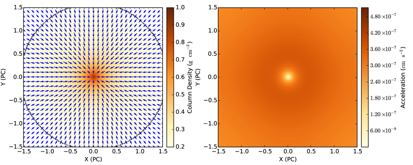
Figure 16: Left Panel: Density distribution and acceleration for our clump model (see Section 4.3 for details). The background image is the density distribution and the vectors stand for acceleration. Right Panel: A map of the magnitude of acceleration.

Fig. 17 correspond to Fig. 5.

Figure 17: Upper Panel: surface density distribution and acceleration of the Pipe region. The background image is the surface density distribution and the vectors stand for acceleration. Lower Panel: A map of the magnitude of acceleration of the same region. Here one degree correspond to $\sim 3\;\rm pc$.

Fig. 18 correspond to Fig. 6.

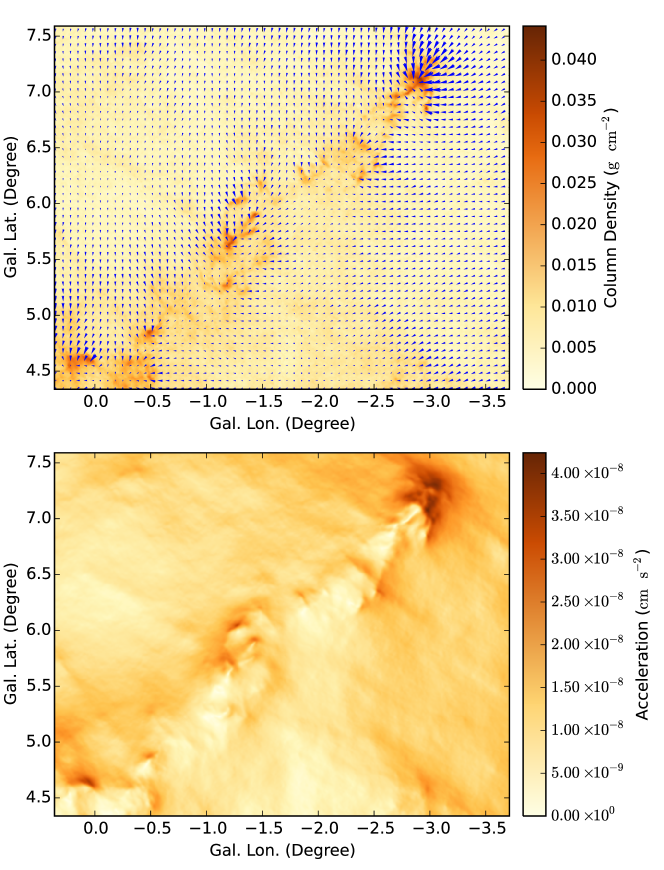
Figure 18: Upper Panel: surface density distribution and acceleration of the Pipe Nebula. The background image is the surface density distribution and the vectors stand for acceleration. Lower Panel: A map of the magnitude of acceleration of the same region. The red stars stand for the YSO candidates in (Forbrich et al., 2009). Here one degree correspond to $\sim 3\;\rm pc$.

Fig. 19 correspond to Fig. 6.

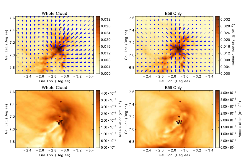
Figure 19: Upper Panels: surface density maps and acceleration of the B59 region in the Pipe Nebula. The background images are the surface density distributions and the vectors stand for acceleration. Lower Panels: Maps of the magnitude of acceleration of the same region. The red stars stand for the YSO candidates in Forbrich et al. (2009). The results shown in the left panels are computed by taking all the matter of the Pipe nebula into account (whole cloud), and the results shown in the right panels are computed by taking only the matter inside the B59 into account (B59 only). Here one degree correspond to $\sim 3\;\rm pc$.

Fig. 20 correspond to Fig. 8.

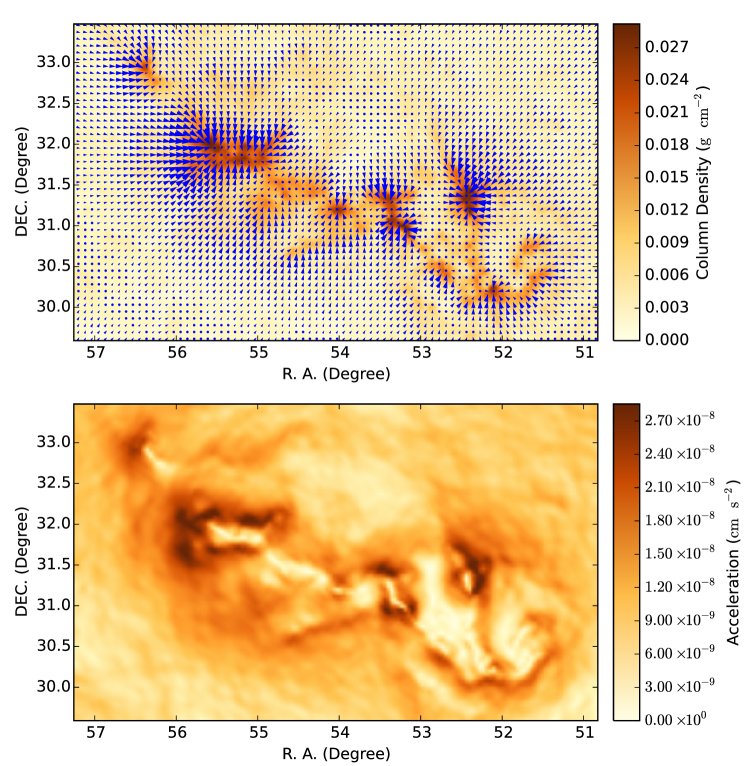
Figure 20: Upper Panel: surface density distribution and acceleration of the Perseus molecular cloud. The background image is the surface density distribution and the vectors stand for acceleration. Lower Panel: A map of the magnitude of acceleration of the same region. Here one degree correspond to $\sim 4.5\;\rm pc$.

Fig. 21 correspond to Fig. 9.

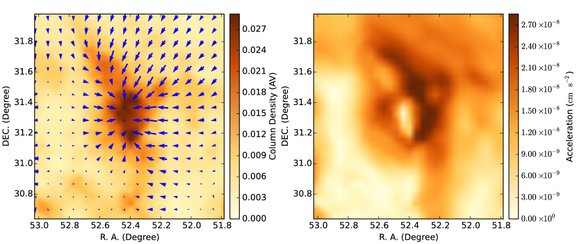
Figure 21: Left Panel: surface density distribution and acceleration of the NGC1333 region in the Perseus molecular cloud. The background image is the surface density distribution and the vectors stand for acceleration. Right Panel: A map of the magnitude of acceleration of the same region. Here one degree correspond to $\sim 4.5\;\rm pc$.

Fig. 22 correspond to Fig. 10.

Figure 22: Upper Panel: surface density distribution and acceleration of the IC348-B3 region in the Perseus molecular cloud. The background image is the surface density distribution and the vectors stand for acceleration. Lower Panel: A map of the magnitude of acceleration of the same region. The blue contours mark the region where starless and prestellar cores are found (Enoch et al., 2006). Here one degree correspond to $\sim 4.5\;\rm pc$.