EFFICIENT EVALUATION OF SCALED PROXIMAL OPERATORS

Abstract

Quadratic-support functions [Aravkin, Burke, and Pillonetto; J. Mach. Learn. Res. 14(1), 2013] constitute a parametric family of convex functions that includes a range of useful regularization terms found in applications of convex optimization. We show how an interior method can be used to efficiently compute the proximal operator of a quadratic-support function under different metrics. When the metric and the function have the right structure, the proximal map can be computed with cost nearly linear in the input size. We describe how to use this approach to implement quasi-Newton methods for a rich class of nonsmooth problems that arise, for example, in sparse optimization, image denoising, and sparse logistic regression.

90C15, 90C25

1 Introduction

The proximal operator is a key ingredient in many convex optimization algorithms for problems with nonsmooth objective functions. Proximal-gradient algorithms in particular are prized for their applicability to a broad range of convex problems that arise in machine learning and signal processing, and for their good theoretical convergence properties. Under reasonable hypotheses they are guaranteed to achieve, within $k$ iterations, a function value that is within $\mathcal{O}(1/k)$ of the optimal value using a constant step size, and within $\mathcal{O}(1/k^{2})$ using an accelerated variant. Tseng [33] outlines a unified view of the many proximal-gradient variations, including accelerated versions such as FISTA [6].

In its canonical form, the proximal-gradient algorithm applies to convex optimization problems of the form

(1.1) $$\mathop{\hbox{minimize}}_{x\in\mathbb{R}^{n}}\quad f(x)+g(x),$$

where the functions $f:\mathbb{R}^{n}\to\mathbb{R}$ and $g:\mathbb{R}^{n}\to\mathbb{R}\cup\{+\infty\}$ are convex. We assume that $f$ has a Lipschitz-continuous gradient, and that $g$ is lower semicontinuous [29, Definition 1.5]. Typically, $f$ is a loss function that penalizes incorrect predictions of a model, and $g$ is a regularizer that encourages desirable structure in the solution. Important examples of nonsmooth regularizers are the 1-norm and total variation, which encourage sparsity in either $x$ or its gradient.

Suppose that $H$ is a positive-definite matrix. The iteration

(1.2) $$x^{+}=\mathbf{prox}^{\scriptscriptstyle H}_{g}(x-H^{-1}\nabla f(x))$$

underlies the prototypical proximal-gradient method, where $x$ is most recent estimate of the solution, and

(1.3) $$\mathbf{prox}^{\scriptscriptstyle H}_{g}(z):=\mathop{\hbox{arg\,min}}_{x\in\mathbb{R}^{n}}\left\{\tfrac{1}{2}\|z-x\|_{\scriptscriptstyle H}^{2}+g(x)\right\}$$

is the (scaled) proximal operator of $g$. The scaled diagonal $H=\alpha I$ is typically used to define the proximal operator because it leads to an inexpensive proximal iteration, particularly in the case where $g$ is separable. (In that case, $\alpha$ has a natural interpretation as a steplength.) More general matrices $H$, however, may lead to proximal operators that dominate the computation. The choice of $H$ remains very much an art. In fact, there is an entire continuum of algorithms that vary based on the choice of $H$, as illustrated by Table 1.1.

Table 1.1: Preconditioned proximal-gradient methods.

Method	Reference	$H$
iterative soft thresholding	[6]	$\alpha I$
symmetric rank 1	[7]	$\alpha I+ss^{T}$
identity-minus-rank-1	[19]	$\alpha I-ss^{T}\!$
proximal L-BFGS	[31, 38, 30]	$\Lambda+SDS^{T}$
proximal Newton	[21, 32, 13]	$\nabla^{2}f$

The table lists a set of algorithms roughly in order of the accuracy with which $H$ approximates the Hessian—when it exists—of the smooth function $f$. At one extreme is iterative soft thresholding (IST), which approximates the Hessian using a constant diagonal. At the other extreme is proximal Newton, which uses the true Hessian. The quality of the approximation induces a tradeoff between the number of expected proximal iterations and the computational cost of evaluating the proximal operator at each iteration. Thus $H$ can be considered a preconditioner for the proximal iteration. The proposals offered by Tran-Dinh et al. [32] and Byrd et al. [13] are flexible in the choice of $H$, and so those references might also be considered to apply to other methods listed in Table 1.1.

The main contribution of this paper is to show how for an important family of functions $g$ and $H$, the proximal operator (1.3) can be computed efficiently via an interior method. This approach builds on the work of Aravkin et al. [2], who define the class of quadratic-support functions and outline a particular interior algorithm for their optimization. Our approach is specialized to the case where the quadratic-support function appears inside of a proximal computation. Together with the correct dualization approach (§4), this yields a particularly efficient interior implementation when the data that define $g$ and $H$ have special structure (§6). The proximal quasi-Newton method serves as a showcase for how this technique can be used within a broader algorithmic context (§7).

2 Quadratic-support functions

Aravkin et al. [2] introduce the notion of a quadratic-support (QS) function, which is a generalization of sublinear support functions [29, Ch. 8E]. Here we introduce a slightly more general definition than the version implemented by Aravkin et al. We retain the “QS” designation because the quadratic term, which is an essential feature of their definition, can also be expressed by the version we use here.

Let $\mathbb{B}_{p}=\set{z}{\|z\|_{p}\leq 1}$ and $\mathcal{K}=\mathcal{K}_{1}\times\cdots\times\mathcal{K}_{k}$, where each cone $\mathcal{K}_{i}$ is either a nonnegative orthant $\mathbb{R}_{+}^{m}$ or a second-order cone $\mathbb{Q}^{m}=\set{(\tau,z)\in\mathbb{R}\times\mathbb{R}^{m-1}}{z\in\tau\mathbb{B}_{2}}$. (The size $m$ of the cones may of course be different for each index $i$.) The notation $Ay\succeq_{\mathcal{K}}b$ means that $Ay-b\in\mathcal{K}$, and $\tau\mathbb{B}_{p}\equiv\set{\tau z}{z\in\mathbb{B}_{p}}$. The indicator on a convex set $U$ is denoted as

$$\delta(x\mid U)=\begin{cases}0&\mbox{if $x\in U$,}\\ +\infty&\mbox{otherwise.}\end{cases}$$

Unless otherwise specified, $x$ is an $n$-vector. To help disambiguate dimensions, the $p$-by-$p$ identity matrix is denoted by $I_{p}$, and the $p$-vector of all ones by $\mathbf{1}_{p}$.

We consider the class of functions $g:\mathbb{R}^{n}\to\mathbb{R}\cup\{+\infty\}$ that have the conjugate representation

(2.1) $$g(x)=\sup_{y\in\mathcal{Y}}\ y^{T}\!(Bx+d),\text{where}\mathcal{Y}=\{y\in\mathbb{R}^{\ell}\mid Ay\succeq_{\mathcal{K}}b\}.$$

(The term “conjugate” alludes to the implicit duality, since $g$ may be considered as the conjugate of the indicator function to the set $\mathcal{Y}$.) We assume throughout that the feasible set $\mathcal{Y}=\set{y}{Ay\succeq_{\mathcal{K}}b}$ is nonempty. If $\mathcal{Y}$ contains the origin, the QS function $g$ is nonnegative for all $x$, and we can then consider it to be a penalty function. This is automatically true, for example, if $b\leq 0$.

The formulation (2.1) is close to the standard definition of a sublinear support function [28, §13], which is recovered by setting $d=0$ and $B=I$, and letting $\mathcal{Y}$ be any convex set. Unlike a standard support function, $g$ is not positively homogeneous if $d\neq 0$. This is a feature that allows us to capture important classes of penalty functions that are not positively homogeneous, such as piecewise quadratic functions, the “deadzone” penalty, or indicators on certain constraint sets. These are examples that are not representable by the standard definition of a support function. Our definition springs from the quadratic-support function definition introduced by Aravkin et al. [2], who additionally allow for an explicit quadratic term in the objective and for $\mathcal{Y}$ to be any nonempty convex set. The concrete implementation considered by Aravkin et al., however, is restricted to the case where $\mathcal{Y}$ is polyhedral. In contrast, we also allow $\mathcal{K}$ to contain second-order cones. Therefore, any quadratic objective terms in the Aravkin et al. definition can be “lifted” and turned into a linear term with a second-order-cone constraint (see Example 2.2). Our definition is thus no less general.

This expressive class of functions includes many penalty functions commonly used in machine learning; Aravkin et al. give many other examples. In addition, they show how to interpret QS functions as the negative log of an associated probability density, which makes these functions relevant to maximum a posteriori estimation. In the remainder of this section we provide some examples that illustrate various regularizing functions and constraints that can be expressed as QS functions.

Example 2.1 (1-norm regularizer).

The 1-norm has the QS representation

$$\|x\|_{1}=\sup_{y}\set{y^{T}\!x}{y\in\mathbb{B}_{\infty}},$$

where

(2.2) $$A=\begin{pmatrix}\phantom{-}I_{n}\\ -I_{n}\end{pmatrix},\quad b=-{\begin{pmatrix}\mathbf{1}_{n}\\ \mathbf{1}_{n}\end{pmatrix}},\quad d=0,\quad B=I_{n},\quad\mathcal{K}=\mathbb{R}_{+}^{2n},$$

_□

Example 2.2 (2-norm).

This simple example illustrates how the QS representation (2.1) can represent the 2-norm, which is not possible using the QS formulation described by Aravkin et al. [2] where the constraints are polyhedral. With our definition, the 2-norm has the QS representation

$$\|x\|_{2}=\sup_{y}\set{y^{T}\!x}{y\in\mathbb{B}_{2}}=\sup_{y}\set{y^{T}\!x}{(1,y)\succeq_{\mathcal{K}}0},$$

where

(2.3) $$A=\begin{pmatrix}0\\ I_{n}\end{pmatrix},\quad b=\begin{pmatrix}1\\ 0\end{pmatrix},\quad d=0,\quad B=I_{n},\quad\mathcal{K}=\mathbb{Q}^{n+1}.$$

_□

Example 2.3 (Polyhedral norms).

Any polyhedral seminorm is a support function, e.g., $\|Bx\|_{1}$ for some matrix $B$. In particular, if the set $\set{y}{Ay\geq b}$ contains the origin and is centro-symmetric, then

$$\|x\|:=\sup_{y}\set{y^{T}\!Bx}{Ay\geq b}$$

defines a norm if $B$ is nonsingular, and a seminorm otherwise. This is a QS function with $d:=0$ (as will be the case for any positively homogeneous QS function) and $\mathcal{Y}:=\set{y}{Ay\geq b}$. _□

Example 2.4 (Quadratic function).

This example justifies the term “quadratic” in our modified definition, even though there are no explicit quadratic terms. It also illustrates the roles of the terms $B$ and $d$. The quadratic function can be written as

$${\textstyle{\frac{1}{2}}}\|x\|_{2}^{2}=\sup_{y,\,t}\Set{\!y^{T}\!x-{\textstyle{\frac{1}{2}}}t}{\|y\|^{2}_{2}\leq t\!}=\sup_{y,\,t}\Set{\!\begin{pmatrix}y\\ t\end{pmatrix}^{T}\!\left[\begin{pmatrix}I_{n}\\ 0\end{pmatrix}x-\begin{pmatrix}0\\ \nicefrac{{1}}{{2}}\end{pmatrix}\right]}{\|y\|_{2}^{2}\leq t\!}.$$

Use the derivation in A to obtain the QS representation with parameters

$$A=\begin{pmatrix}0&\nicefrac{{1}}{{2}}\\ 0&\nicefrac{{1}}{{2}}\\ I_{n}&0\end{pmatrix},\quad b=\begin{pmatrix}{\phantom{-}\nicefrac{{1}}{{2}}}\\ -\nicefrac{{1}}{{2}}\\ \phantom{-}0\end{pmatrix},\quad d=\begin{pmatrix}0\\ \nicefrac{{1}}{{2}}\end{pmatrix},\quad B=\begin{pmatrix}I_{n}\\ 0\end{pmatrix},\quad\mathcal{K}=\mathbb{Q}^{n+2}.$$

_□

Example 2.5 (1-norm constraint).

This example is closely related to the 1-norm regularizer in Example 2.1, except that the QS function is used to express the constraint $\|x\|_{1}\leq 1$ via an indicator function $g=\delta(\,\cdot\mid\mathbb{B}_{1})$. Write the indicator to the 1-norm ball as the conjugate of the infinity norm, which gives

(2.4) $$\delta(x\mid\mathbb{B}_{1}) =\sup_{y}\set{y^{T}\!x-}{y\|_{\infty}}$$

$$=\sup_{y,\,\tau}\set{y^{T}\!x-\tau}{y\in\tau\mathbb{B}_{\infty}}=\sup_{y,\,\tau}\set{y^{T}\!x-\tau}{-\tau\mathbf{1}_{n}\leq y\leq\tau\mathbf{1}_{n}}.$$

This is a QS function with parameters

$$A=\begin{pmatrix}-I_{n}&\mathbf{1}_{n}\\ \phantom{-}I_{n}&\mathbf{1}_{n}\end{pmatrix},\quad b=0,\quad d=\begin{pmatrix}\phantom{-}0\\ -1\end{pmatrix},\quad B=\begin{pmatrix}I_{n}\\ 0\end{pmatrix},\quad\mathcal{K}=\mathbb{R}^{2n}.$$

_□

Example 2.6 (Indicators on polyhedral cones).

Consider the following polyhedral cone and its polar:

$$U=\set{x}{Bx\leq 0}\text{and}U^{\circ}=\set{B^{T}\!y}{y\leq 0}.$$

Use the support-function representation of a cone in terms of its polar to obtain

(2.5) $$\delta(x\mid U)=\delta^{*}(\cdot\mid U^{\circ})(x)=\sup_{y}\set{y^{T}\!Bx}{y\leq 0},$$

which is an example of an elementary QS function. (See Rockafellar and Wets [29] for definitions of the polar of a convex set, and the convex conjugate.) A concrete example is the positive orthant, obtained by choosing $B=I_{n}$. An important example, used in isotonic regression [10], is the monotonic cone

$$U:=\set{x}{x_{i}\geq x_{j},\ \forall(i,j)\in\mathcal{E}},$$

Here, $\mathcal{E}$ is the set of edges in a graph $\mathcal{G}=(\mathcal{V},\mathcal{E})$ that describes the relationships between variables in $\mathcal{V}$. If we set $B$ to be the incidence matrix for the graph, (2.5) then corresponds to the indicator on the monotonic cone $U$. _□

Example 2.7 (Distance to a cone).

The distance to a cone $U$ that is a combination of polyhedral and second-order cones can be represented as a QS function:

$$\inf_{x\in U}\|x-y\|_{2} =\inf_{x}\ \set{\|x-y\|_{2}+\delta(x\mid U)}$$

$$=\big{[}\delta(\cdot\mid\mathbb{B}_{2})+\delta(\cdot\mid U^{\circ})\big{]}^{*}(y)=\ \sup\left\{y^{T}\!x\mid y\in\mathbb{B}_{2}\cap U^{\circ}\right\}.$$

The second equality follows from the relationship between infimal convolution and conjugates [28, §16.4]. When $U$ is the positive orthant, for example, $g(x)=\|\max\{0,\,x\}\|_{2},$ where the max operator is taken elementwise. _□

3 Building quadratic-support functions

Quadratic-support functions are closed under addition, composition with an affine map, and infimal convolution with a quadratic function. In the following, let $g_{i}$ be QS functions with parameters $A_{i}$, $b_{i}$, $d_{i}$, $B_{i}$, and $\mathcal{K}_{i}$ (with $i=0,1,2$). The rules for addition and composition are described in [2], which are here summarized and amplified.

Addition rule

The function

$$h(x):=g_{1}(x)+g_{2}(x)$$

is QS with parameters

$$A=\begin{pmatrix}A_{1}&\\ &A_{2}\end{pmatrix},\quad b=\begin{pmatrix}b_{1}\\ b_{2}\end{pmatrix},\quad d=\begin{pmatrix}d_{1}\\ d_{2}\end{pmatrix},\quad B=\begin{pmatrix}B_{1}\\ B_{2}\end{pmatrix},\quad\mathcal{K}=\mathcal{K}_{1}\times\mathcal{K}_{2}.$$

Concatenation rule

The function

$$h(x):=g_{0}(x^{1})+\cdots+g_{0}(x^{k}),$$

where each partition $x^{i}\in\mathbb{R}^{n}$, is QS with parameters

(3.1) $$(A,\,B)=I_{k}\otimes(A_{0},\,B_{0}),\qquad(b,\,d)=\mathbf{1}_{k}\otimes(b_{0},\,d_{0}),\qquad\mathcal{K}=\mathcal{K}_{0}\times\overset{(k)}{\cdots}\times\mathcal{K}_{0}.$$

where the symbol $\otimes$ denotes the Kronecker product. The rule for concatenation follows from the rule for addition of QS functions.

Affine composition rule

The function

$$h(x):=g_{0}(Px-p)$$

is QS with parameters

$$A=A_{0},\quad b=b_{0},\quad d=d_{0}-B_{0}p,\quad B=B_{0}P.$$

Moreau-Yosida regularization

The Moreau-Yosida envelope of $g_{0}$ is the value of the proximal operator, i.e.,

(3.2) $$\mathbf{env}^{\scriptscriptstyle H}_{g_{0}}(z):=\inf_{x}\set{\tfrac{1}{2}}{z-x\|_{\scriptscriptstyle H}^{2}+g_{0}(x)}.$$

It follows from Burke and Hoheisel [12, Proposition 4.10] that

$$\mathbf{env}^{\scriptscriptstyle H}_{g_{0}}(z)=\sup_{y}\set{y^{T}\!(B_{0}x+d_{0})-{\textstyle{\frac{1}{2}}}y^{T}\!B_{0}H^{-1}B_{0}^{T}\!y}{A_{0}y\succeq_{\mathcal{K}_{0}}b_{0}},$$

which is a QS function with parameters

$$A=\begin{pmatrix}0&\nicefrac{{1}}{{2}}\\ 0&\nicefrac{{1}}{{2}}\\ R&0\\ A_{0}&0\end{pmatrix},\quad b=\begin{pmatrix}\phantom{-}\nicefrac{{1}}{{2}}\\ -\nicefrac{{1}}{{2}}\\ 0\\ b_{0}\end{pmatrix},\quad d=\begin{pmatrix}d_{0}\\ -\nicefrac{{1}}{{2}}\end{pmatrix},\quad B=\begin{pmatrix}B_{0}\\ 0\end{pmatrix},\quad\mathcal{K}=\mathbb{Q}^{n+2}\times\mathcal{K}_{0},$$

with Cholesky factorization $R^{T}\!R=B_{0}H^{-1}B_{0}^{T}$. The derivation is given in A, where we take $Q=B_{0}H^{-1}B_{0}^{T}$.

Example 3.1 (Sums of norms).

In applications of group sparsity [37, 18], various norms are applied to all partitions of $x=(x^{1},\ldots,x^{p})$, which possibly overlap. This produces the QS function

(3.3) $$g(x)=\|x^{1}\|+\cdots+\|x^{p}\|,$$

where each norm in the sum may be different. In particular, consider the case of adding two norms $g(x)=\|x^{1}\|_{\triangledown}+\|x^{2}\|_{\vartriangle}$. (The extension to adding three or more norms follows trivially.) First, we introduce matrices $P_{i}$ that restrict $x$ to partition $i$, i.e., $x^{i}=P_{i}x$, for $i=1,2$. Then

$$g(x)=\|P_{1}x\|_{\triangledown}+\|P_{2}x\|_{\vartriangle}.$$

Then we apply the affine-composition and addition rules to determine the corresponding quantities that define the QS representation of $g$:

$$A=\begin{pmatrix}A_{\triangledown}\\ &A_{\vartriangle}\end{pmatrix},\quad b=\begin{pmatrix}b_{\triangledown}\\ b_{\vartriangle}\end{pmatrix},\quad d=0,\quad B=\begin{pmatrix}B_{\triangledown}P_{1}\\ B_{\vartriangle}P_{2}\end{pmatrix},\quad\mathcal{K}=\mathcal{K}_{\triangledown}\times\mathcal{K}_{\vartriangle},$$

where $A_{i}$, $b_{i}$, $B_{i}$, and $\mathcal{K}_{i}$ (with $i=\triangledown,\vartriangle$) are the quantities that define the QS representation of the individual norms. (Necessarily, $d=0$ because the result is a norm and therefore positive homogeneous.) In the special case where $\|\cdot\|_{\triangledown}$ and $\|\cdot\|_{\vartriangle}$ are both the 2-norm, then $A_{i}$, $b_{i}$, $B_{i}$, and $\mathcal{K}_{i}$ are given by (2.3) in Example 2.2. _□

Example 3.2 (Graph-based 1-norm and total variation).

A variation of Example 3.1 can be used to define a variety of interesting norms, including the graph-based 1-norm regularizer used in machine learning [14], and the isotropic and anisotropic versions of total variation (TV), important in image processing [24]. Let

$$g(x)=\|Nx\|_{G}\quad\text{with}\quad\|z\|_{G}=\sum_{i=1}^{p}\|z^{i}\|_{2},$$

where $z^{i}$ is a partition of $z$ and $N$ is an $m$-by-$n$ matrix. For anisotropic TV and the graph-based 1-norm regularizer, $N$ is the adjacency matrix of a graph, and each partition $z^{i}$ has a single unique element, so $g(x)=\|Nx\|_{1}$. For isotropic TV, each partition captures neighboring pairs of variables, and $N$ is a finite-difference matrix. The QS addition and affine-composition rules can be combined to derive the parameters of $g$. When $p=m$ (i.e., each $z^{i}$ is a scalar), we are summing $n$ absolute-value functions, and we use (2.2) and (3.1) to obtain

(3.4) $$A=I_{m}\otimes\begin{pmatrix}\phantom{-}1\\ -1\end{pmatrix},\quad b=\mathbf{1}_{m}\otimes\begin{pmatrix}-1\\ -1\end{pmatrix},\quad d=0,\quad B=N,\quad\mathcal{K}=\mathbb{R}^{2m}_{+}.$$

Now consider the variation where $p=m/2$, (i.e., each partition has size 2), which corresponds to summing $m/2$ two-dimensional 2-norms. Use (2.3) to obtain

$$A=I_{m/2}\otimes\begin{pmatrix}0\\ I_{2}\end{pmatrix},\quad b=\mathbf{1}_{m/2}\otimes\begin{pmatrix}1\\ 0\end{pmatrix},\quad d=0,\quad B=N,\quad\mathcal{K}=\mathbb{Q}^{2}\times\overset{(m/2)}{\cdots}\times\mathbb{Q}^{2}.$$

_□

4 The proximal operator as a conic QP

We describe in this section how the proximal map (1.2) can be obtained as the solution of a quadratic optimization problem (QP) over conic constraints,

(4.1) $$\displaystyle\mathop{\hbox{minimize}}_{y}\quad\tfrac{1}{2}y^{T}\!Qy-c^{T}\!y\quad\mathop{\hbox{subject to}}\quad Ay\succeq_{\mathcal{K}}b,$$

for some positive semidefinite $\ell$-by-$\ell$ matrix $Q$ and a convex cone $\mathcal{K}=\mathcal{K}_{1}\times\cdots\times\mathcal{K}_{k}$. The transformation to a conic QP is not immediate because the definition of the QS function implies that the proximal map involves nested optimization. Duality, however, furnishes a means for simplifying this problem.

Proposition 4.1.

Let $g$ be a QS function. The following problems are dual pairs:

(4.2a) $$\displaystyle\mathop{\hbox{minimize}}_{x} {\textstyle{\frac{1}{2}}}\|z-x\|^{2}_{\scriptscriptstyle H}+g(x),$$

(4.2b) $$\displaystyle\mathop{\hbox{minimize}}_{Ay\succeq_{\mathcal{K}}b} {\textstyle{\frac{1}{2}}}y^{T}\!BH^{-1}B^{T}y-(d+Bz)^{T}\!y.$$

If strong duality holds, the corresponding primal-dual solutions are related by

(4.3) $$Hx+B^{T}\!y=Hz.$$

Proof.

Let

$$h_{1}(x):=\tfrac{1}{2}\|x-z\|_{H}^{2}\text{and}h_{2}(x):=\sup_{y\in\mathcal{Y}}\set{y^{T}\!(x+d)}.$$

If strong duality holds, it follows from Bertsekas [9, Prop. 5.3.8] that

(4.4) $$\inf_{x}\ h_{1}(x)+h_{2}(Bx)=-\inf_{y}\ h_{1}^{*}(-B^{T}y)+h_{2}^{*}(y),$$

where

$$h_{1}^{*}(y)=\tfrac{1}{2}\|y\|_{H^{-1}}^{2}+z^{T}y\text{and}h_{2}^{*}(y)=\delta(z\mid\mathcal{Y})-d^{T}y$$

are the Fenchel conjugates of $h_{1}$ and $h_{2}$, and the infima on both sides are attained. (See Rockafellar [28, §12] for the convex calculus of Fenchel conjugates.) The right-hand side of (4.4) is precisely the dual problem (4.2b). It also follows from Fenchel duality that the pair $(x,y)$ is optimal only if

$$x\in\mathop{\hbox{arg\,min}}_{x}\set{h_{1}(x)+y^{T}\!Bx}.$$

Differentiate this objective to obtain (4.3).

Strong duality holds when $B\cdot\mbox{ri dom}(h_{1})\cap\mbox{ri dom}(h_{2})\neq\emptyset.$ This holds, for example, when the interior of the domain of $g$ is nonempty, since

$$\mbox{int dom}(g)\neq\emptyset\iff\mbox{im}\,B\cap\mbox{int dom}(h_{2})\neq\emptyset\Rightarrow B\cdot\mbox{ri dom}(h_{1})\cap\mbox{ri dom}(h_{2})\neq\emptyset.$$

In all of the examples in this paper, this holds true.

5 Primal-dual methods for conic QP

Proposition 4.1 provides a means of evaluating the proximal map of QS functions via conic quadratic optimization. There are many algorithms for solving convex conic QPs, but primal-dual methods offer a particularly efficient approach that can leverage the special structure that defines the class of QS functions. A detailed discussion of the implementation of primal-dual methods for conic optimization is given by Vandenberghe [34]; here we summarize the main aspects that pertain to implementing these methods efficiently in our context.

The standard development of primal-dual methods for (4.1) is based on perturbing the optimality conditions, which can be stated as follows. The solution $y$, together with slack and dual vectors $s$ and $v$, must satisfy

$$Qy-A^{T}v=c,\quad v\succeq_{\mathcal{K}}0,\quad Sv=0,$$

where the matrix $S$ is block diagonal, and each $m_{i}$-by-$m_{i}$ block $S_{i}$ is either a diagonal or arrow matrix depending on the type of cone, i.e.,

$$S_{i}=\begin{cases}\operatorname{\bf diag}(s_{i})&\mbox{if $\mathcal{K}_{i}=\mathbb{R}^{m_{i}}_{+}$,}\\ \operatorname{\bf arrow}(s_{i})&\mbox{if $\mathcal{K}_{i}=\mathbb{Q}^{m_{i}}$,}\end{cases}\qquad\operatorname{\bf arrow}(u):=\begin{pmatrix}u_{0}&\bar{u}^{T}\\ \bar{u}&u_{0}I\end{pmatrix}\text{for}u=(u_{0},\bar{u}).$$

See Vandenberghe [34] for further details.

Now replace the complementarity condition $Sv=0$ with its perturbation $Sv=\mu e$, where $\mu$ is a positive parameter and $e=(e^{1},\ldots,e^{k})$, with each partition defined by

$$e^{i}=\begin{cases}(1,1,\ldots,1)&\mbox{if $\mathcal{K}_{i}=\mathbb{R}_{+}^{m_{i}}$,}\\ (1,0,\ldots,0)&\mbox{if $\mathcal{K}_{i}=Q^{m_{i}}$.}\end{cases}$$

A Newton-like method is applied to the perturbed optimality conditions, which we phrase as the root of the function

(5.1) $$R_{\mu}:\begin{pmatrix}y\\ v\\ s\end{pmatrix}\mapsto\begin{pmatrix}r_{d}\\ r_{p}\\ r_{\mu}\end{pmatrix}:=\begin{pmatrix}Qy-A^{T}\!v-c\\ Ay-s-b\\ Sv-\mu e\end{pmatrix}.$$

Each iteration of the method proceeds by systematically choosing the perturbation parameter $\mu$ (ensuring it decreases), and obtaining each search direction as the solution of the Newton system

(5.2) $$\begin{pmatrix}Q&-A^{T}&0\\ A&0&-I\\ 0&S&V\end{pmatrix}\begin{pmatrix}\Delta y\\ \Delta v\\ \Delta s\end{pmatrix}=-{\begin{pmatrix}r_{d}\\ r_{p}\\ r_{\mu}\end{pmatrix}},\qquad\begin{pmatrix}y^{+}\\ v^{+}\\ s^{+}\end{pmatrix}=\begin{pmatrix}y\\ v\\ s\end{pmatrix}+\alpha\begin{pmatrix}\Delta y\\ \Delta v\\ \Delta s\end{pmatrix}.$$

The steplength $\alpha$ is chosen to ensure that $(v^{+},s^{+})$ remain in the strict interior of the cone.

One approach to solving for the Newton direction is to apply block Gaussian elimination to (5.2), and obtain the search direction via the following systems:

(5.3a) $$(Q+A^{T}\!S^{-1}VA)\Delta x =r_{d}+A^{T}\!S^{-1}(Vr_{p}+r_{\mu}),$$

(5.3b) $$\Delta v =S^{-1}(Vr_{p}+r_{\mu}-VA\Delta x),$$

(5.3c) $$\Delta s =V^{-1}\left(r_{\mu}-S\Delta v\right).$$

In practice, the matrices $S$ and $V$ are rescaled at each iteration in order to yield search directions with favorable properties. In particular, the Nesterov-Todd rescaling redefines $S$ and $V$ so that $SV^{-1}=\operatorname{\bf block}(u)$ for some vector $u$, where

(5.4) $$\operatorname{\bf block}(u)_{i}=\begin{cases}\operatorname{\bf diag}(u_{i})&\mbox{if $\mathcal{K}_{i}=\Re_{+}^{m_{i}}$,}\\ (2u_{i}u_{i}^{T}-[u_{i}^{T}\!Ju_{i}]J)^{2}&\mbox{if $\mathcal{K}_{i}=\mathbb{Q}^{m_{i}}$,}\end{cases}\qquad J=\begin{pmatrix}1&0\\ 0&-I_{(m_{i}-1)}\end{pmatrix}.$$

The cost of the overall approach is therefore determined by the cost of solving, at each iteration, linear systems with the matrix

(5.5) $$\mathcal{L}(u):=Q+A^{T}\mbox{\bf{block}}(u)^{-1}A,$$

which now defines the system (5.3a).

6 Evaluating the proximal operator

We now describe how to use Proposition 4.1 to transform a proximal operator (1.3) into a conic QP that can be solved by the interior algorithm described in §5.4. In particular, to evaluate $\mathbf{prox}^{\scriptscriptstyle H}_{g}(x)$ we solve the conic QP (4.1) with the definitions

(6.1) $$Q:=BH^{-1}B^{T},\qquad c:=d+Bx;$$

the other quantities $A$, $b$, and the cone $\mathcal{K}$, appear verbatim. Algorithm 1 summarizes the procedure. As we noted in §5.4, the main cost of this procedure is incurred in Step 1, which requires repeatedly solving linear systems that involve the linear operator (5.5). Together with (6.1), these matrices have the form

(6.2) $$\mathcal{L}(u)=BH^{-1}B^{T}+A^{T}\!\operatorname{\bf block}(u)^{-1}A.$$

Input	: $x$, $H$, and QS function $g$ as defined by parameters $A$, $b$, $d$, $B$, $\mathcal{K}$
Output	: $\mathbf{prox}^{\scriptscriptstyle H}_{g}(x)$

Step 1: Apply interior method to QP (4.2b) to obtain $y^{\star}$.

Step 2: Return $H^{-1}(c-B^{T}\!y^{\star})$.

Algorithm 1 Evaluating $\mathbf{prox}^{\scriptscriptstyle H}_{g}(x)$

Below we offer a tour of several examples, ordered by level of simplicity, to illustrate the details involved in the application of our technique. The Sherman-Woodbury (SW) identity

$$(D+UMU^{T})^{-1}=D^{-1}-D^{-1}U(M^{-1}+U^{T}\!D^{-1}U)^{-1}U^{T}\!D^{-1},$$

valid when $M^{-1}+U^{T}\!D^{-1}U$ is nonsingular, proves useful for taking advantage of certain structured matrices that arise when solving (6.2). Some caution is needed, however, because it is known that the SW identity can be numerically unstable [36].

For our purposes, it is useful to think of the SW formula as a routine that takes the elements ($D,U,M$) that define a linear operator $D+UMU^{T}$, and returns the elements ($D_{1},U_{1},M_{1}$) that define the inverse operator $D_{1}+U_{1}M_{1}U_{1}^{T}=(D+UMU^{T})^{-1}$. We assume that $D$ and $M$ are nonsingular. The following pseudocode summarizes the operations needed to compute the elements of the inverse operator.

function SWinv($D,U,M$)

     1 $D_{1}\leftarrow D^{-1}$

     2 $U_{1}\,\leftarrow D_{1}U$

     3 $M_{1}\leftarrow(M^{-1}+U^{T}\!U_{1})^{-1}$

     4 return $D_{1}$, $U_{1}$, $M_{1}$

      end

Typically, $D$ is a structured operator that admits a fast algorithm for solving linear systems with any right-hand side, and $U$ and $M$ are stored explicitly as dense matrices. Step 1 above computes a new operator $D_{1}$ that simply interchanges the multiplication and inversion operations of $D$. Step 2 applies the operator $D_{1}$ to every column of $U$ (typically a tall matrix with few columns), and Step 3 requires inverting a small matrix.

Example 6.1 (1-norm regularizer; cf. Example 2.1).

Example 2.1 gives the QS representation for $g(x)=\|x\|_{1}$, and the required expressions for $A$, $B$, and $\mathcal{K}$. Because $\mathcal{K}$ is the nonnegative orthant, $\operatorname{\bf block}(u)=\operatorname{\bf diag}(u)$; cf. (5.4). With the definitions of $A$ and $B$, the linear operator $\mathcal{L}$ in (6.2) simplifies to

$$\mathcal{L}(u)=H^{-1}+A^{T}\!\operatorname{\bf diag}(u)A=H^{-1}+\Sigma,$$

where $\Sigma$ is a positive-definite diagonal matrix that depends on $u$. If it happens that the preconditioner $H$ has a special structure such that $H+\Sigma^{-1}$ is easily invertible, it may be convenient to apply the SW identity to obtain equivalent formulas for the inverse

$$\mathcal{L}(u)^{-1}=(H^{-1}+\Sigma)^{-1}=H-H(H+\Sigma^{-1})^{-1}H.$$

Banded, chordal, and diagonal-plus-low-rank matrices are examples of specially structured matrices that make one of these formulas for $\mathcal{L}^{-1}$ efficient. They yield the efficiency because subtracting the diagonal matrix $\Sigma$ preserves the structure of either $H$ or $H^{-1}$. _□

In the important special case where $H=\operatorname{\bf diag}(h)$ is diagonal, each component $i$ of the proximal operator for the 1-norm can be obtained directly via the formula

$$[\mathbf{prox}^{\scriptscriptstyle H}_{g}(x)]_{i}=\operatorname{sign}(x_{i})\cdot\max\{|x_{i}|-1/h_{ii},\,0\},$$

$h_{ii}$ are the diagonal components of $H$. This corresponds to the well-known soft-thresholding operator. There is no simple formula, however, when $H$ is more general.

Example 6.2 (Graph-based 1-norm).

Consider the graph-based 1-norm function from Example 3.2 induced by a graph $\mathcal{G}$ with adjacency matrix $N$. Substitute the definitions of $A$ and $B$ from (3.4) into the formula for $\mathcal{L}$ and simplify to obtain

$$\mathcal{L}(u)=NH^{-1}N^{T}+A^{T}\!\operatorname{\bf diag}(u)A=NH^{-1}N^{T}+\Sigma,$$

where $\Sigma:=A^{T}\!\operatorname{\bf diag}(u)A$ is a positive-definite diagonal matrix. (As with Example 6.1, $\mathcal{K}$ is the positive orthant, and thus $\operatorname{\bf block}(u)=\operatorname{\bf diag}(u)$.) Linear systems of the form $\mathcal{L}(u)p=q$ then can be solved with the following sequence of operations, in which we assume that $H=\Lambda+UMU^{T}$, where $\Lambda$ is diagonal.

1 $(\Lambda_{1},U_{1},M_{1})\leftarrow\texttt{SWinv}(\Lambda,U,M)$

  [ $H^{-1}\equiv\Lambda_{1}+U_{1}M_{1}U_{1}^{T}$ ]

2 $\Sigma_{1}\leftarrow N\Lambda_{1}N^{T}+\Sigma$

3 $(\Sigma_{2},U_{2},M_{2})\leftarrow\texttt{SWinv}(\Sigma_{1},NU_{1},M_{1})$

  [ $\mathcal{L}(u)^{-1}\equiv\Sigma_{2}+U_{2}M_{2}U_{2}^{T}$ ]

4 $p\leftarrow\Sigma_{2}q+U_{2}M_{2}U_{2}^{T}\!q$

  [ solve $\mathcal{L}(u)p=q$ ]

5 return $p$

Observe from the definition of $H$ and the definition of $\Sigma_{1}$ in Step 2 above that

$$\mathcal{L}(u)=\Sigma_{1}+NU_{1}M_{1}U_{1}^{T}N^{T},$$

and then Step 3 computes the quantities that define the inverse of $\mathcal{L}$. The bulk of the work in the above algorithm happens in Step 3, where $\Sigma_{2}\equiv\Sigma_{1}^{-1}$ is applied to each column of $NU_{1}$ (see Step 2 of the SWinv function), and in Step 4, where $\Sigma_{2}$ is applied to $q$. Below we give two special cases where it is possible to take advantage of the structure of $N$ and $H$ in order to apply $\Sigma_{2}$ efficiently to a vector.

1-dimensional total variation.

Suppose that the graph $\mathcal{G}$ is a path. Then the $(n-1)\times n$ adjacecy matrix is given by

$$N=\begin{pmatrix}-1&1\\ &\ddots&\ddots\\ &&-1&1\end{pmatrix}.$$

The matrix $\Sigma_{1}:=N\Lambda^{-1}N^{T}+\Sigma$ (see Step 2 of the above algorithm) is tridiagonal, and hence equations of the form $\Sigma_{1}q=p$ can be solved efficiently using standard techniques, e.g., Golub and Loan [16, Algorithm 4.3.6].

Chordal graphs.

If the graph $\mathcal{G}$ is chordal, than the matrix $N^{T}\!DN$ is also chordal when $D$ is diagonal. This implies that it can be factored in time linear with the number of edges of the graph [1]. We can use this fact to apply $\Sigma_{2}\equiv\Sigma_{1}^{-1}$ efficiently, as follows: let $(\Sigma_{3},U_{3},M_{3})=\texttt{SWinv}(\Sigma,N,\Lambda_{1})$, which implies

$$\Sigma_{2}:=\Sigma_{3}+U_{3}M_{3}U_{3}^{T},\quad\mbox{where}\quad\Sigma_{3}:=\Sigma^{-1},\quad M_{3}:=(N^{T}\!\Sigma^{-1}N+\Lambda_{1})^{-1}.$$

Because $N^{T}\!\Sigma^{-1}N$ is chordal, so is $M_{3}$, and any methods efficient for solving with chordal matrices can be used when applying $\Sigma_{2}$.

_□

Example 6.3 (1-norm constraint; cf. Example 2.5).

Example 2.5 gives the QS representation for the indicator function on the 1-norm ball. Because the constraints on $y$ in (2.4) involve only bound constraints, $\operatorname{\bf block}(u)=\operatorname{\bf diag}(u)$. With the definitions of $A$ and $B$ from Example 2.5, the linear operator $\mathcal{L}$ has the form

$$\mathcal{L}(u)=\begin{pmatrix}0\\ I_{n}\end{pmatrix}H^{-1}\begin{pmatrix}0&I_{n}\end{pmatrix}+\begin{pmatrix}\phantom{-}\mathbf{1}_{n}^{T}&\mathbf{1}_{n}^{T}\\ -I_{n}&I_{n}\end{pmatrix}\begin{pmatrix}\operatorname{\bf diag}(u_{1})\\ &\operatorname{\bf diag}(u_{2})\end{pmatrix}\begin{pmatrix}\mathbf{1}_{n}&-I_{n}\\ \mathbf{1}_{n}&\phantom{-}I_{n}\end{pmatrix},$$

where $u=(u_{1},u_{2})$. Thus, $\mathcal{L}$ simplifies to

$$\mathcal{L}(u)=\begin{pmatrix}\mathbf{1}_{n}^{T}\!u&(u^{-})^{T}\!\\ u^{-}&H^{-1}+\Sigma\end{pmatrix}\hbox{\qquad where\qquad}\Sigma:=\operatorname{\bf diag}(u^{+}),\quad\begin{array}[]{c}u^{+}:=\phantom{-}u_{1}+u_{2},\\ u^{-}:=-u_{1}+u_{2}.\end{array}$$

Systems that involve $\mathcal{L}$ can be solved by pivoting on the block $(H^{-1}+\Sigma)$. The cases where this approach is efficient are exactly those that are efficient in the case of Example 6.1. _□

Example 6.4 (2-norm; cf. Example 2.2).

Example 2.2 gives the QS representation for the 2-norm function. Because $\mathcal{K}=Q^{n}$, then $\operatorname{\bf block}(u)=(2uu^{T}-[u^{T}\!Ju]J)^{2}$, where $u=(u_{0},\bar{u})$ and $J$ is specified in (5.4). With the expressions for $A$ and $B$ from Example 2.2, the linear operator $\mathcal{L}$ reduces to

(6.3) $$\mathcal{L}(u)=H^{-1}+\alpha I_{n}+vv^{T},\text{with}\alpha=(u^{T}\!Ju)^{2},\ v=\sqrt{8u_{0}}\cdot\bar{u}.$$

This amounts to a perturbation of $H^{-1}$ by a multiple of the identity, followed by a rank-1 update. Therefore, systems that involve $\mathcal{L}$ can be solved at the cost of solving systems with $H+\alpha I_{n}$ (for some scalar $\alpha$).

Of course, the proximal map of the 2-norm is easily computed by other means; our purpose here is to use this as a building block for more useful penalties, such as Example 3.1, which involves the sum-of-norms function shown in (3.3). Suppose that the $p$ partitions do not overlap, and have size $n_{i}$ for $i=1,\ldots,p$. The operator $\mathcal{L}$ in (6.3) generalizes to

$$\mathcal{L}(u)=H^{-1}+\underset{W}{\underbrace{\begin{pmatrix}\alpha_{1}I_{n_{1}}+v^{1}(v^{1})^{T}\\ &\ddots\\ &&\alpha_{p}I_{n_{p}}+v^{p}(v^{p})^{T}\end{pmatrix}}}\ ,\quad\begin{aligned} u^{i}&=(u^{i}_{0},\bar{u}^{i})\\ \alpha_{i}&=(u^{iT}Ju^{i})^{2}\\ v^{i}&=\sqrt{8u^{i}_{0}}\cdot\bar{u}^{i},\end{aligned}$$

where each vector $u_{i}$ has size $n_{i}+1$.

When $p$ is large, we can treat each diagonal block of $W$ as an individual (small) diagonal-plus-rank-1 matrix. If $H^{-1}$ is diagonal-plus-low-rank, for example, the diagonal part of $H^{-1}$ can be subsumed into $W$. In that case, each diagonal block in $W$ remains diagonal-plus-rank-1, which can be inverted in parallel by handling each block individually. Subsequently, the inverse of $\mathcal{L}$ can be obtained by a second correction.

Another approach, when $p$ is small, is to consider $W$ as a diagonal-plus-rank-$p$ matrix:

$$W=\begin{pmatrix}\alpha_{1}I_{n_{1}}\\ &\ddots\\ &&\alpha_{p}I_{n_{p}}\end{pmatrix}+\begin{pmatrix}v^{1}\\ &\ddots\\ &&v^{p}\end{pmatrix}\begin{pmatrix}v^{1}\\ &\ddots\\ &&v^{p}\end{pmatrix}^{T}.$$

This representation is convenient: systems involving $\mathcal{L}$ can be solved efficiently in a manner identical to that of Example 6.1 because $W$ is a diagonal-plus-low-rank matrix.

_□

Example 6.5 (separable QS functions).

Suppose that $g$ is separable, i.e.,

$$g(x)=\gamma(x_{1})+\cdots+\gamma(x_{n}),$$

where $\gamma:\mathbb{R}\to\mathbb{R}$ is a QS function with parameters $(A_{\gamma},b_{\gamma},B_{\gamma},d_{\gamma},\mathbb{R}_{+}^{np})$, and $p$ is an integer parameter that depends on $\gamma$. The parameters $A$ and $B$ for $g$ follow from the concatenation rule (3.1), and $A=(I_{n}\otimes A_{\gamma})$ and $B=(I_{n}\otimes B_{\gamma})$. Thus, the linear operator $\mathcal{L}$ is given by

$$\mathcal{L}(u)=(I_{n}\otimes B_{\gamma})H^{-1}(I_{n}\otimes B_{\gamma})^{T}+(I_{n}\otimes A_{\gamma})^{T}\operatorname{\bf diag}(u)(I_{n}\otimes A_{\gamma}).$$

Apply the SW identity to obtain

$$\mathcal{L}(u)^{-1}=\Lambda^{-1}-\Lambda^{-1}(I_{n}\otimes B_{\gamma})(H+\Sigma)^{-1}(I_{n}\otimes B_{\gamma})^{T}\Lambda^{-1},$$

where $\Lambda=\operatorname{\bf diag}(\Lambda_{1},\ldots,\Lambda_{n})$,

$$\Lambda_{i}=A_{\gamma}^{T}\!\operatorname{\bf diag}(u^{i})A_{\gamma},\quad\text{and}\quad\Sigma=\operatorname{\bf diag}(B_{\gamma}^{T}\Lambda_{1}^{-1}B_{\gamma},\dots,B_{\gamma}^{T}\Lambda_{n}^{-1}B_{\gamma}).$$

Because the function $\gamma$ takes a scalar input, $B_{\gamma}$ is a vector. Hence $\Sigma$ is a diagonal matrix. Note too that $\Lambda$ is a block diagonal matrix with $n$ blocks each of size $p$. We can then solve the system $\mathcal{L}(u)p=q$ with the following steps:

1 $q_{1}\leftarrow(I_{n}\otimes B_{\gamma})^{T}\Lambda^{-1}q$

2 $q_{2}\leftarrow(H+\Sigma)^{-1}q_{1}$

3 $q_{3}\leftarrow\Lambda^{-1}q_{2}-\Lambda^{-1}(I_{n}\otimes B_{\gamma})q_{2}$

The cost of solving systems with the operator $\mathcal{L}$ is dominated by solves with the block diagonal matrix $\Lambda$ (Steps 1 and 3) and $H+\Sigma$ (Step 2). The cost of the latter linear solve is explored in Example 6.1. _□

7 A proximal quasi-Newton method

We now turn to the proximal-gradient method discussed in §1. Our primary goal is to demonstrate the feasibility of the interior approach for evaluating proximal operators of QS functions. A secondary goal is to illustrate how this technique leads to an efficient extension of the quasi-Newton method for nonsmooth problems of practical interest.

We follow Scheinberg and Tang [30] and implement a limited-memory BFGS (L-BFGS) variant of the proximal-gradient method that has no linesearch and that approximately evaluates the proximal operator. Scheinberg and Tang establish a sublinear rate of convergence for this method when the Hessian approximations are suitably modified by adding a scaled identity matrix, and when the scaled proximal maps are evaluated with increasing accuracy. In their proposal, the accuracy of the proximal evaluation is based on bounding the value of the approximation to (3.2). We depart from this criterion, however, and instead use the residual (5.1) obtained by the interior solver to determine the required accuracy. In particular, we require that the optimality criterion of the interior algorithm used to evaluate the operator is a small multiplicative constant $\kappa$ of the current optimality of the outer proximal-gradient iterate, i.e.,

$$\|R_{\mu}(y,v,s)\|\leq\kappa\|x_{k}-\mathbf{prox}_{g}(x_{k}-\nabla f(x_{k}))\|.$$

This heuristic is reminiscent of the accuracy required of the linear solves used by an inexact Newton method for root finding [15]. Note that the proximal map $\mathbf{prox}_{g}\equiv\mathbf{prox}^{\scriptscriptstyle I}_{g}$ used above is unscaled, which in many cases can be easily computed when $g$ is seperable.

7.1 Limited-memory BFGS updates

Here we give a brief outline the L-BFGS method for obtaining Hessian approximations of a smooth function $f$. We follow the notation of Nocedal and Wright [25, §6.1], who use $H_{k}$ to denote the current approximation to the inverse of the Hessian of $f$. Let $x_{k}$ and $x_{k+1}$ be two consecutive iterates, and define the vectors

$$s_{k}=x_{k+1}-x_{k},\quad\text{and}\quad y_{k}=\nabla f(x_{k+1})-\nabla f(x_{k}).$$

A “full memory” BFGS method updates the approximation $H_{k}$ via the recursion

$$H_{0}=\sigma I,\qquad H_{k+1}=H_{k}-\frac{H_{k}s_{k}s_{k}^{T}H_{k}}{s_{k}^{T}H_{k}s_{k}}+\frac{y_{k}y_{k}^{T}}{y_{k}^{T}s_{k}},$$

for some positive parameter $\sigma$ that defines the initial approximation. The limited-memory variant of the BFGS update (L-BFGS) maintains the most recent $m$ pairs $(s_{k},y_{k})$, discarding older vectors. In all cases, $m\ll n$, e.g., $m=10$. The globalization strategy advocated by Scheinberg and Tang [30] may add a small multiple of the identity to $H_{k}$. This modification takes the place of a potentially expensive linesearch, and the correction is increased at each iteration if a certain condition for decrease is not satisfied.

Each interior iteration for evaluating the proximal operator depends on solving linear systems with $\mathcal{L}$ in (6.2). In all of the experiments presented below, each interior iteration has a cost that is linear in the number of variables $n$.

8 Numerical experiments

We have implemented the proximal quasi-Newton method as a Julia package [11], called QSip, designed for problems of the form (1.1), where $f$ is smooth and $g$ is a QS function. The code is available at the URL

https://github.com/MPF-Optimization-Laboratory/QSip.jl

A primal-dual interior method, based on ideas from the CVXOPT software package [1], is used for Algorithm 1. We consider below several examples. The first three examples apply the QSip solver to minimize benchmark least-squares problems with different nonsmooth regularizers that are QS representable; the last example applies the solver to a sparse logistic-regression problem on a standard data set.

8.1 Timing the proximal operator

The examples that we explored in §6 have a favorable structure that allows each interior iteration for evaluating the proximal map $\mathbf{prox}^{\scriptscriptstyle H}_{g}(x)$ to scale linearly with problem size. In this section we verify this behavior empirically for problems with the structure

(8.1) $$H=I+UU^{T},\qquad g(x)=\|x\|_{1},\qquad U\in\mathbb{R}^{n\times k}$$

for different values of $k$ and $n$. This choice of diagonal-plus-low-rank matrices is designed to mimic the structure of matrices that appear in L-BFGS. Here $U$ and $x$ are chosen with random normal entries. As described in Example 2.1, the system $\mathcal{L}(u)$ is inverted in linear time using the SW identity.

We evaluate the proximal map on $100$ random instances for each combination of $k$ and $n$, and plot in Figure 1 the average time needed to reach an accuracy of $10^{-7}$, as measured by the optimality conditions in the interior algorithm. Because in practice the number of iterations of the interior method is almost independent of the size of the problem, the time taken to compute the proximal map is a predictable, linear function of the size of the problem.

Figure 8.1: Time taken to compute $\mathbf{prox}^{\scriptscriptstyle H}_{g}(x)$ versus $n$, for $k=1,10,100$; see (8.1).

8.2 Synthetic least-square problems

The next set of examples all involve the least-squares objective

(8.2) $$f(x)={\textstyle{\frac{1}{2}}}\|Ax-b\|^{2}_{2}.$$

Two different procedures are used to construct matrices $A$, as described in the following sections. In all cases, we follow the testing approach described by Lorenz [23] for constructing a test problem with a known solution: fix a vector $x^{\star}$ and choose $b=Ax^{\star}-A^{-T}v$, where $v\in\partial g(x^{\star})$. Note that

$$\partial(f+g)(x^{\star})=A^{T}(Ax^{\star}-[Ax^{\star}-A^{-T}v])+\partial g(x^{\star})=\partial g(x^{\star})-v.$$

Because $v\in\partial g(x^{\star})$, the above implies that $0\in\partial(f+g)(x^{\star})$, and hence $x^{\star}$ minimizes the objective $f+g$. In the next three sections, we apply QSip in turn to problems with $g$ equal to the 1-norm, the group LASSO (i.e., sum of 2-norm functions), and total variation.

8.2.1 One-norm regularization

In this experiment we choose $g=\|\cdot\|_{1}$, which gives the 1-norm regularized least-squares problem, often used in applications of sparse optimization. Following the details in Example 2.1, the system $\mathcal{L}(u)$ is a diagonal-plus-low-rank matrix, which we invert using the SW identity.

The matrix $A$ in (8.2) is a 2000-by-2000 lower triangular matrix with all nonzero entries equal to $1$. The bandwidth $p$ of $A$ is adjustable, and determines its coherence

$$\mbox{coherence}(A)=\max_{i\neq j}\frac{a_{i}^{T}\!a_{j}}{\|a_{i}\|\|a_{j}\|}=\sqrt{\frac{p-1}{p}},$$

where $a_{i}$ is the $i$th column. As observed by Lorenz [23], the difficulty of 1-norm regularized least-squares problems are strongly influenced by the coherence. Our experiments use matrices $A$ with bandwidth $p=500,1000,2000$.

Figure 8.2 shows the results of applying the QSip solver with a memories $k=1,10$, labeled “QSIP mem $=k$”. We also consider comparisons against two competitive proximal-based methods. The first is a proximal-gradient algorithm that uses the Barzilai-Borwein steplength [5, 35]. This is our own implementation of the method, and is labeled “Barzilai-Borwein” in the figures. The second is the proximal quasi-Newton method implemented by Becker and Fadili [7], which is based on a symmetric-rank-1 Hessian approximation; this code is labeled “PG-SR1”. The QSip solver with memory of 10 outperforms the other solvers. The quasi-Newton approximation benefits problems with high coherence ($p$ large) more than problems with low coherence ($p$ small). In all cases, the experiments reveal that the additional cost involved in evaluating a proximal operator (via an interior method) is balanced by the overall cost of the algorithm, both in terms of iterations (i.e., matrix-vector products with $A$) and time.

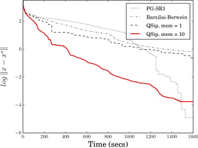
Figure 8.2: Performance of solvers applied to 1-norm regularized least-squares problems of increasing difficulty. The left and right columns, respectively, track the distance of the current solution estimate to the true solution versus time and iteration number. Top row: $p=2000$ (highest coherence); middle row: $p=1000$; bottom row: $p=500$ (lowest coherence).

8.2.2 The effect of conditioning

It is well known that the proximal-gradient method converges slowly for ill conditioned problems. The proximal L-BFGS method may help to improve convergence in such situations. We investigate the observed convergence rate of the proximal L-BFGS approach on a family of least-squares problems with 1-norm regularization with varying degrees of ill conditioning. For these experiments, we take $A$ in (8.2) as the 2000-by-2000 matrix

$$A=\alpha_{L}\begin{pmatrix}T&0\\ 0&0\end{pmatrix}+\alpha_{\mu}I,$$

where $T$ is a 1000-by-1000 tridiagonal matrix with constant diagonal entries equal to 2, and constant sub- and super-diagonal entries equal to ${-}1$. The parameter $\alpha_{\scriptscriptstyle L}/\alpha_{\mu}$ controls the conditioning of $A$, and hence the conditioning of the Hessian $A^{T}\!A$ of $f$.

We run L-BFGS with 4 different memories (“mem”): $0$ (i.e., proximal gradient with a Barzilai-Borwein steplength), $1$, $10$, and $100$. We terminate the algorithm either when the error drops beneath $10^{-8}$, or the method reaches $10^{3}$ iterations. Our method of measuring the observed convergence (OC) computes the line of best fit to the log of optimality versus $k$, which results in the quantity

$$\mbox{Observed Convergence}:=\frac{\sum_{k=0}^{N}k\cdot\log\|x_{k}-x_{*}\|}{\sum_{k=0}^{N}\log\|x_{k}-x_{*}\|},$$

where $N$ is the total number of iterations.

The plot in Figure 8.3 shows the ratio of the OC for L-BFGS relative to the observed convergence of proximal gradient (PG). This quantity can be interpreted the amount of work that a single quasi-Newton step performs relative to the number of PG iterations. The plot reveals that the quasi-Newton method is faster at all condition numbers, but is especially effective for problems with moderate conditioning. Also, using a higher quasi-Newton memory almost always lowers the number of iterations. This benefit is most pronounced when the problem conditioning is poor.

Together with §8.1, this section gives a broad picture of the trade-off between the proximal quasi-Newton and proximal gradient methods. The time required for each proximal gradient iteration is dominated by the cost of the gradient computation because the evaluation of the unscaled proximal operator is often trivial. On the other hand, the proximal quasi-Newton iteration additionally requires evaluating the scaled proximal operator. Therefore, the proximal quasi-Newton method is most appropriate when this cost is small relative to the gradient evaluation.

Figure 8.3: Performance of the proximal quasi-Newton method relative to proximal gradient for problems of varying condition number.

8.2.3 Group LASSO

Our second experiment is based on the sum-of-norms regularizer described in Examples 3.1 and 6.4. In this experiment, the $n$-vector (with $n=2000$) is partitioned into $p=5$ disjoint blocks of equal size. The matrix $A$ is fully lower triangular.

Figure 8.4 clearly shows that the QSip solver outperforms the PG method with the Barzilai-Borwein step size. Although we required QSip to exit with a solution estimate accurate within 6 digits (i.e., $\log\|x-x^{*}\|\leq 10^{-6}$), the interior solver failed to achieve the requested accuracy because of numerical instability with the SW formula used for solving the Newton system. This raises the question of how to use efficient alternatives to the SW update that are numerically stable and can still leverage the structure of the problem.

Figure 8.4: Performance of solvers applied to a group-Lasso problem. The horizontal axis measures elapsed time; the vertical axis measures distance to the solution.

8.2.4 1-dimensional total variation

Our third experiment sets

$$g(x)=\sum_{i=1}^{n-1}|x_{i+1}-x_{i}|,$$

which is the anisotropic total-variation regularizer described in Examples 3.2 and 6.2. The matrix $A$ is fully lower triangular. Figure 8.5 compares the convergence behavior of QSip with the Barzilai-Borwein proximal solver. The Python package prox-tv [3, 4] was used for the evaluation of the (unscaled) proximal operator, needed by the Barzilai-Borwein solver. The QSip solver, with memories of 1 and 10, outperformed the Barzilai-Borwein solver.

Figure 8.5: Performance of the QSip solver applied to a 1-dimensional total-variation problem.

8.3 Sparse logistic regression

This next experiment tests QSip on the sparse logistic-regression problem problem

$$\mathop{\hbox{minimize}}_{x}\quad\frac{1}{N}\sum_{i=1}^{N}\log(1+\exp[a_{i}^{T}\!x])+\lambda\|x\|_{1},$$

where $N$ is the number of observations. The Gisette [17] and Epsilon [27] datasets, standard benchmarks from the UCI Machine Learning Repository [22], are used for the feature vectors $a_{i}$. Gisette has $5K$ parameters and $13.5K$ observations; Epsilon has $2K$ parameters with $400K$ observations. These datasets were chosen for their large size and modest number of parameters. In all of these experiments, $\lambda=0.01$.

Figure 8.6 compares QSip to the Barzilai-Borwein solver, and to newGLMNet [20], a state-of-the-art solver for sparse logistic regression. (Other possible comparisons include the implementation of Scheinberg and Tang [30], which we do not include because of difficulty compiling that code.) Because we do not know a priori the solution for this problem, the vertical axis measures the log of the optimality residual $\|x_{k}-\mathbf{prox}_{g}(x_{k}-\nabla f(x_{k}))\|_{\infty}$ of the current iterate. (The norm of this residual necessarily vanishes at the solution.) On the Gisette dataset, Barzilai-Borwein and newGLMNNet are significantly faster than the proximal quasi-Newton implementation. On the Epsilon dataset, however, the quasi-Newton is faster at all levels of accuracy.

Figure 8.6: Performance of solvers on a sparse logistic-regression problem. Top row: Gisette dataset; bottom row: Epsilon dataset. The left and right columns, respectively, track the optimality of the current solution estimate versus elapsed time and iteration number.

9 Conclusion

Much of our discussion revolves around techniques for solving the Newton systems (5.2) that arise in the implementation of an interior method for solving QPs. The Sherman-Woodbury formula features prominently because it is a convenient vehicle for taking advantage of the structure of the Hessian approximations and the structured matrices that typically define QS functions. Other alternatives, however, may be preferable, depending on the application.

For example, we might choose to reduce the 3-by-3 matrix in (5.2) to an equivalent symmetrized system

$$\begin{pmatrix}-Q&A^{T}\\ A&D\end{pmatrix}\begin{pmatrix}\Delta y\\ \Delta s\end{pmatrix}=-\begin{pmatrix}-{r_{d}}\\ r_{p}+V^{-1}r_{\mu}\end{pmatrix}$$

with $D:=V^{-1}S$. As described by Benzi and Wathen [8], Krylov-based method, such as MINRES [26], may be applied to a preconditioned system, using the preconditioner

$$P=\begin{pmatrix}-\mathcal{L}(u)\\ &D\end{pmatrix},$$

where $\mathcal{L}(u)$ is defined in (5.5). This “ideal” preconditioner clusters the spectrum into three distinct values, so that in exact arithmetic, MINRES would converge in three iterations. The application of the preconditioner requires solving systems with $\mathcal{L}$ and $D$, and so all of the techniques discussed in §6 apply. One benefit, however, which we have not explored here, is that the preconditioning approach allows us to approximate $\mathcal{L}^{-1}(u)$, rather than to compute it exactly, which may yield computational efficiencies for some problems.

Appendix A QS Representation for a quadratic

Here we derive the QS representation of a support function that includes an explicit quadratic term:

$$g(x)=\sup_{y}\set{y^{T}\!(B_{0}x+d_{0})-{\textstyle{\frac{1}{2}}}y^{T}\!Qy}{A_{0}y\succeq_{\mathcal{K}_{0}}b_{0}}.$$

Let $R$ be such that $R^{T}\!R=Q$. We can then write the quadratic function in the objective as a constraint its epigraph, i.e.,

$$g(x)=\sup_{y,\,t}\set{y^{T}\!(B_{0}x+d_{0})-{\textstyle{\frac{1}{2}}}t}{A_{0}y\succeq_{\mathcal{K}}b_{0},\ \|Ry\|^{2}\leq t}.$$

Next we write the constraint $\|Ry\|^{2}\leq t$ as a second-order cone constraint:

$$\|Ry\|^{2}\leq t \iff\|Ry\|^{2}\leq\frac{(t+1)^{2}-(t-1)^{2}}{4}$$

$$\iff\|Ry\|^{2}+\left(\frac{t-1}{2}\right)^{2}\leq\left(\frac{t+1}{2}\right)^{2}$$

$$\iff\sqrt{\|Ry\|^{2}+\left(\frac{t-1}{2}\right)^{2}}\leq\frac{t+1}{2}$$

$$\iff\left\|\begin{pmatrix}0&\nicefrac{{1}}{{2}}\\ R&0\end{pmatrix}\begin{pmatrix}y\\ t\end{pmatrix}+\begin{pmatrix}-\nicefrac{{1}}{{2}}\\ 0\end{pmatrix}\right\|\leq\frac{t+1}{2}$$

$$\iff\begin{pmatrix}0&\nicefrac{{1}}{{2}}\\ 0&\nicefrac{{1}}{{2}}\\ R&0\end{pmatrix}\begin{pmatrix}y\\ t\end{pmatrix}\preceq_{Q}\begin{pmatrix}\phantom{-}\nicefrac{{1}}{{2}}\\ \ -\nicefrac{{1}}{{2}}\\ 0\end{pmatrix}.$$

Concatenating this with the original constraints gives a QS function with parameters

$$A=\begin{pmatrix}0&\nicefrac{{1}}{{2}}\\ 0&\nicefrac{{1}}{{2}}\\ R&0\\ A_{0}&0\end{pmatrix},\quad b=\begin{pmatrix}{\phantom{-}\nicefrac{{1}}{{2}}}\\ -\nicefrac{{1}}{{2}}\\ 0\\ b_{0}\end{pmatrix},\quad d=\begin{pmatrix}d_{0}\\ -\nicefrac{{1}}{{2}}\end{pmatrix},\quad B=\begin{pmatrix}B_{0}\\ 0\end{pmatrix},\quad\mathcal{K}=\mathbb{Q}^{n+2}\times\mathcal{K}_{0}.$$

References

- Andersen et al. [2010] M. Andersen, J. Dahl, and L. Vandenberghe. Implementation of nonsymmetric interior-point methods for linear optimization over sparse matrix cones. Mathematical Programming Computation, 2(3-4):167–201, 2010.
- Aravkin et al. [2013] A. Y. Aravkin, J. V. Burke, and G. Pillonetto. Sparse/robust estimation and Kalman smoothing with nonsmooth log-concave densities: Modeling, computation, and theory. J. Mach. Learn. Res., 14(1):2689–2728, 2013.
- Barbero and Sra [2011] A. Barbero and S. Sra. Fast Newton-type methods for total variation regularization. In L. Getoor and T. Scheffer, editors, ICML, pages 313–320. Omnipress, 2011. URL http://dblp.uni-trier.de/db/conf/icml/icml2011.html#JimenezS11.
- Barbero and Sra [2014] A. Barbero and S. Sra. Modular proximal optimization for multidimensional total-variation regularization, 2014. arXiv 0902.0885.
- Barzilai and Borwein [1988] J. Barzilai and J. M. Borwein. Two-point step size gradient methods. IMA J. Numer. Anal., 8:141–148, 1988.
- Beck and Teboulle [2009] A. Beck and M. Teboulle. A fast iterative shrinkage-thresholding algorithm for linear inverse problems. SIAM Journal on Imaging Sciences, 2(1):183–202, 2009.
- Becker and Fadili [2012] S. Becker and J. Fadili. A quasi-Newton proximal splitting method. In F. Pereira, C. Burges, L. Bottou, and K. Weinberger, editors, Advances in Neural Information Processing Systems 25, pages 2618–2626. Curran Associates, Inc., 2012.
- Benzi and Wathen [2008] M. Benzi and A. J. Wathen. Some preconditioning techniques for saddle point problems. In Model order reduction: theory, research aspects and applications, pages 195–211. Springer, 2008.
- Bertsekas [2009] D. P. Bertsekas. Convex optimization theory. Athena Scientific Belmont, MA, 2009.
- Best and Chakravarti [1990] M. J. Best and N. Chakravarti. Active set algorithms for isotonic regression; a unifying framework. Math. Program., 47(1):425–439, 1990. ISSN 1436-4646. 10.1007/BF01580873.
- Bezanson et al. [2014] J. Bezanson, A. Edelman, S. Karpinski, and V. B. Shah. Julia: A fresh approach to numerical computing, November 2014.
- Burke and Hoheisel [2013] J. V. Burke and T. Hoheisel. Epi-convergent smoothing with applications to convex composite functions. SIAM J. Optim., 23(3):1457–1479, 2013.
- Byrd et al. [2016] R. H. Byrd, J. Nocedal, and F. Oztoprak. An inexact successive quadratic approximation method for L-1 regularized optimization. Math. Program., 157(2):375–396, 2016. ISSN 1436-4646. 10.1007/s10107-015-0941-y. URL http://dx.doi.org/10.1007/s10107-015-0941-y.
- Chin et al. [2013] H. H. Chin, A. Madry, G. L. Miller, and R. Peng. Runtime guarantees for regression problems. In Proceedings of the 4th conference on Innovations in Theoretical Computer Science, pages 269–282. ACM, 2013.
- Dembo et al. [1982] R. S. Dembo, S. C. Eisenstat, and T. Steihaug. Inexact Newton methods. SIAM J. Numer. Anal., 19(2):400–408, 1982.
- Golub and Loan [1989] G. H. Golub and C. F. V. Loan. Matrix Computations. Johns Hopkins University Press, Baltimore, second edition, 1989.
- Guyon et al. [2004] I. Guyon, S. Gunn, A. Ben-Hur, and G. Dror. Result analysis of the NIPS 2003 feature selection challenge. Advances in Neural Information Processing Systems, 17:545–552, 2004.
- Jenatton et al. [2010] R. Jenatton, J. Mairal, F. R. Bach, and G. R. Obozinski. Proximal methods for sparse hierarchical dictionary learning. In Proceedings of the 27th International Conference on Machine Learning (ICML-10), pages 487–494, 2010.
- Karimi and Vavasis [2014] S. Karimi and S. Vavasis. IMRO: a proximal quasi-Newton method for solving -regularized least square problem, 2014.
- Kim et al. [2007] S.-J. Kim, K. Koh, M. Lustig, S. Boyd, and D. Gorinevsky. An interior-point method for large-scale L1-regularized least squares. IEEE J. Sel. Top. Signal Process., 1(4):606–617, 2007.
- Lee et al. [2014] J. D. Lee, Y. Sun, and M. A. Saunders. Proximal Newton-type methods for minimizing composite functions. SIAM J. Optim., 24(3):1420–1443, 2014.
- Lichman [2013] M. Lichman. UCI machine learning repository, 2013. URL http://archive.ics.uci.edu/ml.
- Lorenz [2013] D. A. Lorenz. Constructing test instances for basis pursuit denoising. IEEE Trans. Sig. Proc., 61(5):1210–1214, March 2013.
- Lou et al. [2014] Y. Lou, T. Zeng, S. Osher, and J. Xin. A weighted difference of anisotropic and isotropic total variation model for image processing. Technical report, Department of Mathematics, UCLA, 2014.
- Nocedal and Wright [1999] J. Nocedal and S. J. Wright. Numerical Optimization. Springer, New York, 1999.
- Paige and Saunders [1975] C. C. Paige and M. A. Saunders. Solution of sparse indefinite systems of linear equations. SIAM J. Numer. Anal., 12(4):617–629, 1975.
- [27] Pascal Large Scale Learning Challenge. http://largescale.ml.tu-berlin.de/instructions, 2016. Accessed: 2016-11-22.
- Rockafellar [1970] R. T. Rockafellar. Convex Analysis. Princeton University Press, Princeton, 1970.
- Rockafellar and Wets [1998] R. T. Rockafellar and R. J. B. Wets. Variational Analysis, volume 317. Springer, 1998. 3rd printing.
- Scheinberg and Tang [2016] K. Scheinberg and X. Tang. Practical inexact proximal quasi-Newton method with global complexity analysis. Mathematical Programming, 160(1):495–529, 2016. ISSN 1436-4646. 10.1007/s10107-016-0997-3. URL http://dx.doi.org/10.1007/s10107-016-0997-3.
- Schmidt et al. [2009] M. Schmidt, E. van den Berg, M. P. Friedlander, and K. Murphy. Optimizing costly functions with simple constraints: a limited-memory projected quasi-Newton algorithm. In Proc. 12th Inter. Conf. Artificial Intelligence and Stat., pages 448–455, April 2009.
- Tran-Dinh et al. [2015] Q. Tran-Dinh, A. Kyrillidis, and V. Cevher. Composite self-concordant minimization. Journal of Machine Learning Research, 16:371–416, 2015. URL http://jmlr.org/papers/v16/trandihn15a.html.
- Tseng [2010] P. Tseng. Approximation accuracy, gradient methods, and error bound for structured convex optimization. Math. Program., 125:263–295, 2010.
- Vandenberghe [2010] L. Vandenberghe. The CVXOPT linear and quadratic cone program solvers, 2010.
- Wright et al. [2009] S. J. Wright, R. D. Nowak, and M. A. Figueiredo. Sparse reconstruction by separable approximation. IEEE Transactions on Signal Processing, 57(7):2479–2493, 2009.
- Yip [1986] E. Yip. A note on the stability of solving a rank-p modification of a linear system by the Sherman-Morrison-Woodbury formula. SIAM J. Sci. Stat. Comput., 7(2):507–513, 1986.
- Yuan and Lin [2006] M. Yuan and Y. Lin. Model selection and estimation in regression with grouped variables. J. Royal Stat. Soc. B., 68, 2006.
- Zhong et al. [2014] K. Zhong, E.-H. Yen, I. S. Dhillon, and P. K. Ravikumar. Proximal quasi-Newton for computationally intensive l1-regularized m-estimators. In Z. Ghahramani, M. Welling, C. Cortes, N. Lawrence, and K. Weinberger, editors, Advances in Neural Information Processing Systems 27, pages 2375–2383. Curran Associates, Inc., 2014.