Norm-1 Regularized Consensus-based ADMM for Imaging with a Compressive Antenna

Abstract

This paper presents a novel norm-one-regularized, consensus-based imaging algorithm, based on the Alternating Direction Method of Multipliers (ADMM). This algorithm is capable of imaging composite dielectric and metallic targets by using limited amount of data. The distributed capabilities of the ADMM accelerates the convergence of the imaging. Recently, a Compressive Reflector Antenna (CRA) has been proposed as a way to provide high-sensing-capacity with a minimum cost and complexity in the hardware architecture. The ADMM algorithm applied to the imaging capabilities of the Compressive Antenna (CA) outperforms current state of the art iterative reconstruction algorithms, such as Nesterov-based methods, in terms of computational cost; and it ultimately enables the use of a CA in quasi-real-time, compressive sensing imaging applications.

I Introduction

Reducing the cost of electromagnetic sensing and imaging systems is a necessity before they can be ubiquitously deployed as a part or a large-scale network of sensors. Recently, a single transceiver Compressive Antenna (CA) was proposed as a vehicle to enhance the sensing capacity of an active imaging system, which is equivalent to maximizing the information transfer efficiency from the imaging domain and radar system; and, as a result, the cost and hardware architecture of the imaging system can be drastically reduced [1]. This unique feature of CAs has triggered its use in a wide variety of applications, which include the following: 1) active imaging of metallic target at mm-wave frequencies [1]; passive imaging of the physical temperature of the earth at mm-wave frequencies [2]; and active imaging of red blood cells at optical frequencies [3]. CAs rely on the use of norm-one-regularized iterative Compressive Sensing imaging techniques (CS), such as NESTA [4], which are slow and computationally very expensive; and, ultimately, it may compromise its use in quasi-real-time imaging applications. In order to overcome these imaging barriers, a new fully-parallelizable, consensus-based imaging algorithm, based on the Alternating Direction Method of Multipliers (ADMM) formulation is proposed in this paper.

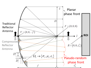
Figure 1: 2D cross-section of a Traditional Reflector Antenna (${x>0}$), and Compressive Reflector Antenna (${x<0}$).

II Compressive Reflector Antenna

II-A General Overview

The concept of operation of the CRA for sensing and imaging applications relies on two basic principles: 1) multi-dimensional codification, generated by a customized reflector; and 2) compressing sensing imaging, performed on the measured data.

The CRA is fabricated, as Fig. 1 shows on the bottom ($x<0$), by introducing discrete scatterers, $\Omega_{i}$, on the surface of a Traditional Reflector Antenna (TRA), shown on the top ($x>0$) of Fig. 1. Each scatterer $\Omega_{i}$ is characterized by the electromagnetic parameters: conductivity, permeability and permittivity, $\{\sigma_{i},\mu_{i},\epsilon_{i}\}$, and the scatterer size $\{D_{i}^{x},D_{i}^{y},D_{i}^{z}\}$ in $\{\bf\hat{x},\hat{y},\hat{z}\}$. CRA and TRA share also many geometrical parameters: $D$, aperture size; $f$, focal length; $h_{o}$, offset height.

These scatterers generate a spatially coded pattern in the near and far field of the antenna after reflecting the incident field produced by the feeding element. When this coded pattern is changed as a function of time, CS techniques can be used to generate a 3D image of an object under test. There are several techniques that may be used for switching among different spatial coded patterns generated by the CRA. Some of them are the following: 1) electronic beam steering by using a focal plane array; 2) electronic beam steering by an electronically-reconfigurable sub-reflector; 3) electronic change of the constitutive parameters of the scatters; 4) mechanical rotation of the reflector along the axis of the parabola $\bf\hat{z}$; 5) mechanical rotation of a single feeding horn or array along the axis of the parabola $\bf\hat{z}$.

II-B Sensing matrix

For the example carried out in this paper, a mechanical rotation of the reflector along the axis of the parabola is chosen to generate the coded pattern, so just with a single transceiver the CRA can perform the 3D imaging. This configuration can be described as a multiple mono-static one, in which data is collected during the scan period, $t_{s}$, where the reflector is rotated $\theta_{r}$ degrees for $r=1,...,N_{\theta}$ along the axis of the parabola. The image reconstruction, which is placed on a Region Of Interest (ROI) located $z_{0}^{T}$ meters away of the focal point of the CRA, is performed in $N_{p}$ pixels and the systems uses $N_{f}$ frequencies. Under this configuration, the sensing matrix $\textbf{H}\in{\mathbb{C}}^{N_{t}\times N_{p}}$ establishes a linear relationship between the unknown complex vector $\textbf{u}\in{\mathbb{C}}^{N_{p}}$ and the measured complex field data $\textbf{g}\in{\mathbb{C}}^{N_{t}}$, with $N_{t}=N_{\theta}\cdot N_{f}$, the total number of reflector rotation angles times the number of frequencies. This relationship can be expressed in a matrix form as follows:

$$\bf{g=Hu+w},$$ (1)

where $\textbf{w}\in\mathbb{C}^{N_{t}}$ represents the noise collected by the receiving antenna for a given frequency and rotation angle.

III ADMM formulation

Equation (1) can be solved via a novel method for optimizing convex functions called the Alternating Direction Method of Multipliers (ADMM), [5, 6]. The general representation of an optimization problem through the ADMM takes the following form:

$$\left.\begin{array}[]{c}\mbox{minimize $f(\textbf{u})+g(\textbf{v})$}\\ \mbox{$\;\;\;$s.t.$\;\;\;\;\;\;\bf{Pu+Qv=c}$}\end{array}\right.$$ (2)

where $f$ and $g$ are convex, closed and proper functions over the unknown vectors $\textbf{u}\in{\mathbb{C}}^{n}$ and $\textbf{v}\in{\mathbb{C}}^{m}$, and the known matrices $\textbf{P}\in{\mathbb{C}}^{p\times n}$ and $\textbf{Q}\in{\mathbb{C}}^{p\times m}$ and vector $\textbf{c}\in{\mathbb{C}}^{p}$ are the ones that define the constraint. As it can be noticed, the methodology of ADMM introduces a new variable v in order to be able to update both variables u and v in an alternating direction fashion. The price to pay for this is the need to add a new constraint. A detail description about the ADMM may be found in the references [5, 7, 8]. In order to solve equation (1) for the unknown variable u, the convex function $f(\textbf{u})=\left\|\bf{Hu-g}\right\|_{2}^{2}$ is minimized in conjuntion with the norm 1 regularized $g(\textbf{v})=\lambda\left\|\textbf{v}\right\|_{1}$; as a result, the ADMM problem to minimize takes the lasso form and is formulated as follows:

$$\left.\begin{array}[]{cc}\mbox{minimize}&\frac{1}{2}\left\|\bf{Hu-g}\right\|_{2}^{2}+\lambda\left\|\textbf{v}\right\|_{1}\\ \mbox{s.t.}&\bf{u-v=0},\end{array}\right.$$ (3)

where $\bf{P=I}$, $\bf{Q=-I}$ and $\bf{c=0}$ enforces that the variables u and v are equal. This problem can be solved in a distributed fashion, by splitting the original matrix $\bf{H}$ and the vector $\bf{g}$ into $N$ submatrices $\textbf{H}_{i}$ –by rows– and $N$ sub-vectors $\textbf{g}_{i}$, as shown in Fig. 2. Additionally, it is possible to define $N$ different variables $\textbf{u}_{i}$; so that the equation (3) turns into

$$\left.\begin{array}[]{cc}\mbox{minimize }&\frac{1}{2}\sum\limits_{i=1}^{N}\left\|\textbf{H}_{i}\textbf{u}_{i}-\textbf{g}_{i}\right\|_{2}^{2}+\lambda\left\|\textbf{v}\right\|_{1}\\ \mbox{s.t.}&\textbf{u}_{i}=\textbf{v},\;\;\forall i=1,...,N.\end{array}\right.$$ (4)

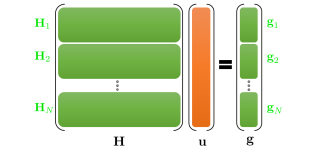
Figure 2: Division of the system by rows.

Equation (4) is solved as $N$ different problems. The variable $\bf{v}$ works as a consensus variable, imposing the agreement between all the variables $\textbf{u}_{i}$. See for example [9, 10, 11, 12, 13]. The augmented Lagrangian function for this problem is of the following form:

$$L\left(\textbf{u}_{i},\textbf{v},\textbf{s}_{i}\right)=\frac{1}{2}\sum\limits_{i=1}^{N}\left\|\textbf{H}_{i}\textbf{u}_{i}-\textbf{g}_{i}\right\|_{2}^{2}+\lambda\left\|\textbf{v}\right\|_{1}+$$

$$+\frac{\rho}{2}\sum\limits_{i=1}^{N}\left\|\textbf{u}_{i}-\textbf{v}+\textbf{s}_{i}\right\|_{2}^{2}-\frac{\rho}{2}\sum\limits_{i=1}^{N}\left\|\textbf{s}_{i}\right\|_{2}^{2}.$$ (5)

where $\textbf{s}_{i}$ is the dual variable for each constraint $i$, and $\rho$ is the augmented parameter that enforces the convexity of the function. This problem can be solved by the following iterative scheme:

$$\textbf{u}_{i}^{k+1} = \left(\textbf{H}_{i}^{\ast}\textbf{H}_{i}+\rho\textbf{I}\right)^{-1}\left(\textbf{H}_{i}^{\ast}\textbf{g}_{i}+\rho\left(\textbf{v}^{k}-\textbf{s}_{i}^{k}\right)\right),$$ (6)

$$\textbf{v}^{k+1} = \mathbf{S}_{\frac{\lambda}{\rho N}}\left(\bar{\textbf{u}}^{k+1}+\bar{\textbf{s}}^{k}\right),$$ (7)

$$\textbf{s}_{i}^{k+1} = \textbf{s}_{i}^{k}+\textbf{u}_{i}^{k+1}-\textbf{v}^{k+1},$$ (8)

where $\mathbf{S}_{\kappa}\left(a\right)$ is the soft thresholding operator [14, 15] interpreted elementwise, defined as follows:

$$\mathbf{S}_{\kappa}\left(a\right)=\left\{\begin{array}[]{c}a-\kappa\ \ \ \ \ a>\kappa,\\ 0\ \ \ \ \ \ \ \ \ \left|a\right|\leq\kappa,\\ a+\kappa\ \ \ \ a<-\kappa,\end{array}\right.$$ (9)

$\bar{\textbf{u}}$ and $\bar{\textbf{s}}$ are the mean of $\textbf{u}_{i}$ and $\textbf{s}_{i}$, respectively, for all $i$. The variable $\bf{v}$ is used to impose the consensus, by using all the independent solutions $\textbf{u}_{i}$ and $\textbf{s}_{i}$. The term $\left(\textbf{H}_{i}^{\ast}\textbf{H}_{i}+\rho\textbf{I}\right)^{-1}$ requires the inversion of a $N_{t}\times N_{t}$ matrix, which is computationally expensive. However, the matrix inversion lemma [16] can be applied in order to perform $N$ inversions of matrices of reduced size $\frac{N_{p}}{N}\times\frac{N_{p}}{N}$, as equation (10) shows:

$$\left(\textbf{H}_{i}^{\ast}\textbf{H}_{i}+\rho\textbf{I}_{N_{t}}\right)^{-1}=\frac{\textbf{I}_{N_{t}}}{\rho}-\frac{\textbf{H}_{i}^{\ast}}{\rho^{2}}\left(\textbf{I}_{\frac{N_{p}}{N}}+\frac{\textbf{H}_{i}\textbf{H}_{i}^{\ast}}{\rho}\right)^{-1}\textbf{H}_{i}$$ (10)

where $\textbf{I}_{N_{t}}$ and $\textbf{I}_{\frac{N_{p}}{N}}$ indicates the identity matrices of sizes $N_{t}$ and ${\frac{N_{p}}{N}}$, respectively.

TABLE I: Parameters for the numerical example.

PARAM.	CONFIG.	PARAM.	CONFIG.
$\lambda_{c}$	$5\cdot 10^{-3}m$	$\theta_{r}$	$90^{\circ}$
$D$	$200\lambda_{c}$	$N_{f}$	$3$
$\left\langle D^{x}\right\rangle=\left\langle D^{y}\right\rangle$	$1.5\lambda_{c}$	$N_{p}$	$25000$
$D_{i}^{z}$	$U\left(\pm 0.54\lambda_{c}\right)$	$z_{0}^{T}$	$195\lambda_{c}$
$f$	$200\lambda_{c}$	$\Delta x_{0}^{T}$	$36\lambda_{c}$
$h_{0}$	$0\lambda_{c}$	$\Delta y_{0}^{T}$	$36\lambda_{c}$
$N_{t}$	$93$	$\Delta z_{0}^{T}$	$7.5\lambda_{c}$
$N_{\theta}$	$31$	$l$	$1.5\lambda_{c}$

IV Numerical Results

The performance of the CRA is evaluated in a millimeter-wave imaging application. The parameters used for the numerical simulation are shown in Table I, as defined in [1]. The total number of measurements used for the reconstruction is given by the number of angles times the number of frequencies, which is equal to 93. The center frequency of the system is 60GHz, and it has a bandwidth of 6GHz. For this example, each scatter $\Omega_{i}$ is considered as a Perfect Electric Conductor (PEC), so $\sigma_{i}=\sigma_{PEC}$ and the CRA is discretized into triangular patches, as described in [17]. These triangles are characterized by an averaged size of $<D^{x}>$ and $<D^{y}>$ in $\bf\hat{x}$ and $\bf\hat{y}$ dimensions, respectively. The scatterer size $D_{i}^{z}$ of each triangle in $\bf\hat{z}$ is modeled as a uniform random variable. The parameter $\lambda_{c}$ is the wavelength at the center frequency. The imaging ROI is located $z^{T}_{0}$ away from the focal point of the CRA; and it encloses a volume determined by the following dimensions: $\Delta x^{T}_{0}$, $\Delta y^{T}_{0}$ and $\Delta z^{T}_{0}$ in $\bf\hat{x}$, $\bf\hat{y}$ and $\bf\hat{z}$ dimensions. The ROI is discretized into cubes of side length $l$.

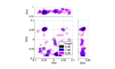
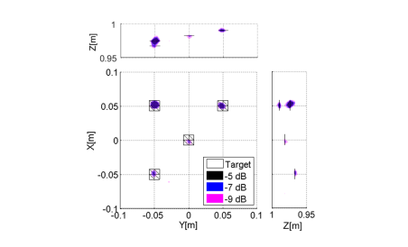
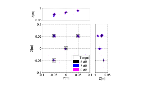
Figure 3: Imaging reconstruction (top, front and side views) using (a) pseudoinverse, (b) NESTA, (c) ADMM. The targets are represented with the transparent black triangles and the reconstructed reflectivity is presented in the colored map.

With the paremeters shown in Table I, the sensing matrix $\bf{H}$ has a size of $93\times 25000$. The proposed method divides $\bf{H}$ into $N=31$ submatrices of size $3\times 25000$, which is used for each optimization of $\textbf{u}_{i}$. As a result of applying the matrix inversion lemma, only $31$ matrices of dimension $3\times 3$ need to be inverted instead of a large $25000\times 25000$ matrix. The inversion of these $31$ matrices are performed just once; and they are used afterwards in each iteration, as indicated in equation (6). The proposed ADMM algorithm highly accelerates the optimization process. Figure 3 shows the imaging results using (a) a traditional pseudo-inverse approach, where many artifacts appear, (b) NESTA algorithm [4] and (c) the ADMM method, with a norm-1 weight of $\lambda=0.01$ and a value of $\rho=1$, for a structure of 4 targets. Despite a few artifacts may appear in this process, the regularized ADMM solution clearly outperforms the pseudo-inverse solution in terms of image quality. Additionally, the ADMM algorithm solved the problem in just 3s for 500 iterations, while the NESTA algorithm solved the problem in 203s, thus showing the efficacy of the proposed approach. In Fig. 4, the ADMM convergence process for different values of the parameters $\lambda$ and $\rho$ is shown, including the combination used for the example in this paper. The stability and speed of the convergence prove that the imaging could be performed in real time.

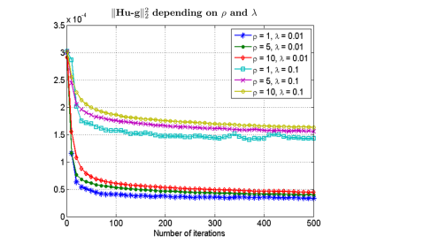
Figure 4: Convergence of ADMM solution for different parameters.

V Conclusion

This work has presented the mathematical principles of a new distributed, consensus-based imaging algorithm using the norm-one-regularized ADMM for a Compressive Reflector Antenna. The explanation of the whole methodology, the graphical comparison between other techniques and the convergence process have been explained in this paper. Besides the simplicity of the proposed algorithm, it outperforms both traditional pseudo-inverse imaging algorithms, in terms of image quality, and current state of the art iterative algorithms (i.e. NESTA), in terms of computational cost.

References

- [1] J. Martinez Lorenzo, J. Heredia Juesas, and W. Blackwell, “A single-transceiver compressive reflector antenna for high-sensing-capacity imaging,” IEEE Antennas and Wireless Propagation Letters, September 2015.
- [2] A. Molaei, G. Allan, J. Heredia, W. Blackwell, and J. Martinez-Lorenzo, “Interferometric sounding using a compressive reflector antenna,” in Antennas and Propagation (EUCAP 2016), 2016.
- [3] H. Gomez-Sousa, O. Rubinos-Lopez, and J. A. Martinez-Lorenzo, “Hematologic characterization and 3d imaging of red blood cells using a compressive nano-antenna and ml-fma modeling,” in Antennas and Propagation (EUCAP2016), 2016.
- [4] S. Becker, J. Bobin, and E. J. Candès, “Nesta: a fast and accurate first-order method for sparse recovery,” SIAM Journal on Imaging Sciences, vol. 4, no. 1, pp. 1–39, 2011.
- [5] S. Boyd, N. Parikh, E. Chu, B. Peleato, and J. Eckstein, “Distributed optimization and statistical learning via the alternating direction method of multipliers,” Foundations and Trends® in Machine Learning, vol. 3, no. 1, pp. 1–122, July 2011.
- [6] S. Boyd and L. Vandenberghe, Convex optimization. Cambridge university press, 2009.
- [7] H. H. Bauschke, R. S. Burachik, P. L. Combettes, V. Elser, D. R. Luke, and H. Wolkowicz, Fixed-Point Algorithms for Inverse Problems in Science and Engineering. Springer, 2011, vol. 49.
- [8] B. He, H. Yang, and S. Wang, “Alternating direction method with self-adaptive penalty parameters for monotone variational inequalities,” Journal of Optimization Theory and applications, vol. 106, no. 2, pp. 337–356, August 2000.
- [9] M. H. DeGroot, “Reaching a consensus,” Journal of the American Statistical Association, vol. 69, no. 345, pp. 118–121, 1974.
- [10] T. Erseghe, D. Zennaro, E. Dall’Anese, and L. Vangelista, “Fast consensus by the alternating direction multipliers method,” Signal Processing, IEEE Transactions on, vol. 59, no. 11, pp. 5523–5537, November 2011.
- [11] J. F. Mota, J. Xavier, P. M. Aguiar, and M. Puschel, “Distributed basis pursuit,” Signal Processing, IEEE Transactions on, vol. 60, no. 4, pp. 1942–1956, April 2012.
- [12] J. F. Mota, J. M. Xavier, P. M. Aguiar, and M. Puschel, “D-admm: A communication-efficient distributed algorithm for separable optimization,” Signal Processing, IEEE Transactions on, vol. 61, no. 10, pp. 2718–2723, May 2013.
- [13] P. A. Forero, A. Cano, and G. B. Giannakis, “Consensus-based distributed support vector machines,” The Journal of Machine Learning Research, vol. 11, pp. 1663–1707, 2010.
- [14] A. Beck and M. Teboulle, “A fast iterative shrinkage-thresholding algorithm for linear inverse problems,” SIAM Journal on Imaging Sciences, vol. 2, no. 1, pp. 183–202, 2009.
- [15] K. Bredies and D. A. Lorenz, “Linear convergence of iterative soft-thresholding,” Journal of Fourier Analysis and Applications, vol. 14, no. 5-6, pp. 813–837, October 2008.
- [16] M. A. Woodbury, “Inverting modified matrices,” Memorandum report, vol. 42, p. 106, 1950.
- [17] J. Meana, J. Martinez-Lorenzo, F. Las-Heras, and C. Rappaport, “Wave scattering by dielectric and lossy materials using the modified equivalent current approximation (meca),” Antennas and Propagation, IEEE Transactions on, vol. 58, no. 11, pp. 3757–3761, Nov 2010.