Phase field modeling of partially saturated deformable porous media

Abstract

A poromechanical model of partially saturated deformable porous media is proposed based on a phase field approach at modeling the behavior of the mixture of liquid water and wet air, which saturates the pore space, the phase field being the saturation (ratio). While the standard retention curve is expected still to provide the intrinsic retention properties of the porous skeleton, depending on the porous texture, an enhanced description of surface tension between the wetting (liquid water) and the non-wetting (wet air) fluid, occupying the pore space, is stated considering a regularization of the phase field model based on an additional contribution to the overall free energy depending on the saturation gradient. The aim is to provide a more refined description of surface tension interactions.

An enhanced constitutive relation for the capillary pressure is established together with a suitable generalization of Darcy’s law, in which the gradient of the capillary pressure is replaced by the gradient of the so-called generalized chemical potential, which also accounts for the “force”  associated to the local free energy of the phase field model. A micro-scale heuristic interpretation of the novel constitutive law of capillary pressure is proposed, in order to compare the envisaged model with that one endowed with the concept of average interfacial area.

The considered poromechanical model is formulated within the framework of strain gradient theory in order to account for possible effects, at laboratory scale, of the micro-scale hydro-mechanical couplings between highly-localized flows (fingering) and localized deformations of the skeleton (fracturing).

Introduction

The constitutive characterization of partially saturated porous media became of interest at the beginning of the last century when scientific research started to face fundamental problems in geotechnics and petroleum engineering, concerning modeling the response of partially imbibed soils, during imbibition/drainage cycles (see [14, 82]), or modeling the behavior of sedimentary reservoir rocks, when a multi-phase fluid flows through the porous network. Starting from the analysis of basic static problems, it became clear that the balance between capillary and driving forces, in particular gravitational forces, would have been the central subject of modeling efforts. This pushed the research in the direction of finding out simple relations between the curvature of the wetting/non-wetting fluid interface and the average content of the wetting fluid, over a suitably defined Representative Volume Element (RVE). The main ideas of this identification have been clearly sketched by [30, Chapter 6] for a partially saturated truncated conical pore, specifying the infinitesimal variation of the interfacial energy in terms of the infinitesimal variation of the volume occupied by the wetting fluid (saturation). This naturally provided the well-known definition of macro-scale capillary pressure, as the derivative of a macro-scale capillary energy. In [69], [13], in the summarizing contribution by [6], in [97] etc., different semi-empirical relations, between macro-scale capillary pressure and saturation have been stated, in order to specify the retention properties of the porous skeleton. These retention curves typically exhibit hysteresis during imbibition/drainage cycles, so as to fit with experimental evidence.

At the same time the pioneering papers by Cahn and Hilliard [16, 17, 18] established the basic framework within which modeling of multi-phase fluid flow is formulated in terms of space and time evolution of the mass concentration or, in the general case, of a phase field which can vary continuously over thin interfacial layers. Beyond the original formulation due to [16] one can refer to [62] and [66] for general reviews, as well as to [71], [11], [12] or [67]. Surface tension is recovered, in this context, considering the integral, through the thickness of the layer, of the concentration gradient (or the gradient of the phase field). This approach progressively attracted more and more interest, in particular within the framework of fluid mechanics, because of its advantages for numerical calculations which do not necessitate adaptive interface fitting grids, see e.g. [62, 66, 52]. Surprisingly however limited contributions attempted at incorporating these ideas into modeling of unsaturated porous media, one can refer for instance to [79] and [80] and more recently to [37, 38, 33] and [53].

This paper follows the research path traced by these authors to model partially saturated deformable porous media, considering the pore network infused with a two-phase fluid. Also the constitutive characterization of the solid will be generalized with respect to the classical poromechanical model, in order to describe the coupling between highly localized flows and (possibly localized) strains.

For long time the above mentioned constitutive characterization of the macro-scale capillary pressure in terms of the corresponding hysteretic retention curve has been the only relation used for describing the hydraulic flow through partially saturated porous media, being also the pivot of the hydro-mechanical coupling with the constitutive law of the porous skeleton. Due to the coarse simplification provided by this model, however, it was finally recognized the existence of several problems in which the relation between capillary pressure and saturation is not sufficient to describe at the same time surface tension, between the wetting and the non-wetting fluid, and the retention properties of the porous skeleton, due to its texture. As a matter of fact what is understood by this constitutive law is, as already mentioned, that no variation of the capillary pressure can be observed if no change of the saturation is induced by external forces. This is due to the rough upscaling rule, from the micro to the macro-scale, which assumes the variation of the area of interfaces proportional to the volume occupied by the fluids, see [30]. On the other hand, as originally pointed out by [75], redistribution of the fluids within a porous medium can occur also keeping constant the saturation, and instabilities can even arise from fluid interfaces that are unable to change curvature smoothly with variations in pressure (“Haines jumps”). In other words, different micro-scale configurations of interfaces between a wetting and a non-wetting phase are possible for a given saturation.

In more refined macro-scale formulations the specific cumulative measure of interfaces, between the wetting and the non-wetting phase, say the specific interfacial area, is also introduced to account for the micro-scale features of the fluids within the RVE, see [59] and the related literature, e.g. [81, 79, 76]. In order to clarify the meaning of this additional macro-scale state parameter, one can think of the effect of the saturation degree, on the macro-scale capillary pressure, as that which coarsely accounts for the retention characteristics of the porous skeleton, depending on its texture, and consider on the other hand the effect of the cumulative measure of interfaces as a suitable corrective term, which allows for describing different admissible coexistence configurations of the saturating fluids. Within this framework, several experimental campaigns have been carried out, based on laboratory tests, see e.g. [40, 39, 28], and also pore network micro-scale numerical simulations have been implemented, see e.g. [64], in order to characterize the constitutive relation among capillary pressure, saturation and specific interfacial area.

Consider now the behavior of the porous skeleton, it is almost standard in continuum poromechanics to introduce a constitutive prescription of stress in terms of strain and saturation, both in the case of elastic and elasto-plastic deformations; one can refer among others to the seminal paper by [1] and the related literature, see e.g. [78, 2], to the systematic formulation by [70], see also [85, 86], to the approach based on the generalized Bishop effective stress, see e.g. [61, 50, 15, 65, 95] etc., or to some recent contributions within the range of finite deformations of the porous skeleton, see [8] and [93]. Possible modifications of these constitutive models, in order to account for the effect of the specific interfacial area, concern the improvement of the retention curve provided within the approach to multi-phase mechanics proposed by [58, 59], in which velocities of phases and interfaces are employed to describe fluid flow and skeleton deformation, see also [55, 56, 77]. Within this framework, however, several phenomena, related to micro-structure remodeling, can not be captured, exactly as several phenomena related to the spatial distribution of fluids within the pores could not be described only in terms of saturation evolution. The typical case is that of localized deformations which have been observed in laboratory scale experimental tests, since the beginning of the 70s, initially using medical scanners for imaging sand bodies, see e.g. [98] and [46], and later with the aid of RX computerized tomography and Digital Image Correlation, see e.g. [45, 68, 57] etc. Thanks to the improvements in the resolving power of tomographs as well as to the progressively increasing skills of scientists in the treatment of experimental data, dry and (partially) saturated specimens have been imaged under triaxial loading conditions to observe localized deformations and porosity change, see e.g. [4, 5] and [44].

In order to model the effects at the scale of the specimen of these micro-scale grain displacements, and in particular to obtain the regularization of localized deformation patterns, the gradient theory of elasto-plasticity, as well as the gradient approach to damage and fracture mechanics, have been adopted in the literature. Typical references are [94], [20] and [73], as well as [49] and [9, 10]. In all these cases however the hydro-mechanical coupling, if any, still remains restricted to the constitutive prescription of the effective or net stress, see e.g. [26] and [92].

As already mentioned, in this paper a novel general approach is developed, within the framework of continuum poromechanics, which aims at merging phase field modeling of multi-phase fluid flow with unsaturated strain gradient poromechanics. While the standard retention curve is expected still to provide the intrinsic retention properties of the porous skeleton, depending on the porous texture, an enhanced description of surface tension between the wetting and the non-wetting fluid, occupying the pore space, is stated considering a regularized phase field model (in the sense of [16]). Similarly to the model which introduces the specific interfacial area as a corrective term of the standard retention curve, this alternative formulation allows for detecting variations of capillary forces even when no change in saturation is caused by the external loading. Indeed a similar approach has already been addressed in the literature, attempting at modeling gravitational fingering and saturation overshooting, through an undeformable porous skeleton, or viscous fingering through a Hele-Shaw cell, see [33, 35, 36]. However no account has been taken of the possible coupling with the deformations of the porous skeleton. In the model which is going to be presented in this paper, on the other hand, the behavior of the solid skeleton is described by means of a strain gradient model, to predict localized strains and fracture, when considering irreversible processes. To the best of author’s knowledge, no general model accounting for both the above mentioned items, say localization in fluid flow and strain, can be retrieved from the literature, except a preliminary study by the author [87], stemming from previous results on modeling of porous media saturated by quasi-incompressible fluids, see [42, 88, 89] and [21, 22, 23, 24, 25]. Within this enhanced framework, the hydro-mechanical coupling is therefore responsible not only for the effects of average variations of the hydraulic regime within the RVE on the skeleton deformation, and vice-versa, see among others [78, 3, 95, 19, 83, 84], but it can also account for the effects of capillary fingering on damaging and fracturing of the skeleton and vice-versa for the effects of strain localization on permeability variations and heterogeneous/anisotropic fluid flow.

The paper is organized as follows: in section 1 the basics of kinematics of (partially) saturated porous media are summarized. In section 2 the expression of the virtual working of external forces, relative to a second gradient multi-phase continuum, is manipulated to obtain the virtual working of internal forces, which is consistent with the balance of the overall momentum. In section 3 the first and the second principle of thermodynamics are introduced in order to get the generalized form of the Clausius-Duhem inequality, prescribing the solid, fluid and thermal dissipations. In section 4, the constitutive laws for the effective stress and hyper-stress are established, considering the contribution of strain and saturation gradients to the overall free energy of the porous continuum; the generalized Darcy law is also deduced. Section 5 is devoted to discuss the properties of the so-called pore-fluid, constitutively characterized in terms of a suitable double well potential, specifying the two phases of the fluid within the pores. In section 6 the generalized prescription of the macro-scale capillary pressure is placed, accounting for its dependence on the saturation gradient. In section 7 the governing equations, say the overall balance law and the generalized Darcy law, are deduced by means of a variational approach which also provides the proper boundary conditions. Finally in section 8 some conclusions are stated.

1 Kinematics

A macroscopic description of kinematics is adopted, treating the partially saturated porous medium as the superposition of a skeleton and a binary mixture of liquid water and wet air. The current placement of the skeleton particles is provided by the deformation of a reference configuration $\mathcal{D}_{0}$. The partial saturation of the pore space is accounted for thinking of the fluid mixture as a non-uniform fluid in the sense of [16], i.e. a fluid possibly having a spatial variation in one of its intensive scalar properties.

Let $\chi_{\alpha}:\mathcal{D}_{0}\times\mathcal{I}\rightarrow\mathtt{I}\!\mathtt{E}$ be the $\alpha$-th component of the deformation (placement) of the skeleton particles with respect to a fixed orthonormal frame in the Euclidean space $\mathtt{I}\!\mathtt{E}$ of positions; $\mathcal{D}_{0}$ is the reference configuration of the solid constituent and $\mathcal{I}$ a time interval. The image of $\mathcal{D}_{0}$ under the deformation map is the current configuration of the porous medium, say $\mathcal{D}\subset\mathtt{I}\!\mathtt{E}$. Moreover let $u_{\alpha}$ indicate the displacement of the solid particles, $F_{\alpha i}=\chi_{\alpha,i}$ the deformation gradient, along the $i$-th direction of an orthonormal frame in the reference configuration of the solid, and $E_{ij}:=\left(F_{\alpha i}F_{\alpha j}-\delta_{ij}\right)/2$ the associated strain tensor, $\delta_{ij}$ being the Kronecker delta. From now on Greek indices label the components of any $n$-th order tensor with respect to a frame in the Euclidean space, whilst Latin indices label the components of any $n$-th order tensor with respect to a frame into the reference configuration of the skeleton $\mathcal{D}_{0}$. Finally let $v_{s}^{\alpha}$ be the $\alpha$-th component of the velocity of the skeleton particles. As usual within the framework of poromechanics, the notions of Eulerian porosity $n$ and Lagrangian porosity $\phi$ are introduced, as the current pore volume density per unit volume of the porous continuum, and the current pore volume density per unit reference volume, respectively. Clearly $\phi=J\,n$; $J$ being the determinant of $F$.

Concerning the non-uniform fluid the intensive scalar property, used from now on to characterize the biphasic characteristic of the fluid, is not the mass concentration but the volume density of the liquid phase with respect to the volume of the pores, say the degree of saturation. The liquid phase of the mixture (water) is assumed incompressible and the gaseous phase (wet air) is assumed to be passive (that is, have infinite mobility) so that its density can be neglected with respect to that of the liquid, $\rho_{L}$; the apparent density of the fluid mixture, say the mass density of the non-uniform fluid per unit volume of the porous medium, is therefore definitely prescribed in terms of the volumetric liquid content $\theta$. If $S_{r}$ indicates the saturation degree (saturation ratio), measuring the current volume occupied by the liquid per unit volume of the pores, the liquid content is $\theta=n\,S_{r}$ and the fluid apparent density is $(n\,\rho_{f})=\rho_{L}(n\,S_{r})=\rho_{L}\,\theta$. The saturation degree ranges within the interval $[0,1]$, where $S_{r}=0$ and $S_{r}=1$ indicate the gaseous and the liquid phase, respectively. The kinematics of the non-uniform fluid is specified as in [89]; the reference placement of the non-uniform fluid particles is therefore prescribed by means of a regular map $g:\mathcal{D}_{0}\times\mathcal{I}\rightarrow\mathcal{D}_{0}^{f}$ defined on the reference configuration of the skeleton. It identifies the fluid material particle within a reference domain $\mathcal{D}_{0}^{f}$, which occupies, at time $t$, the same current place as the solid particle, chosen in $\mathcal{D}_{0}$. Accordingly the fluid velocity coincides with the time derivative of $\chi^{f}(\cdot,t):=\chi(\cdot,t)\circ g(\cdot,t)^{-1}$, which means for every reference particle $X\in\mathcal{D}_{0}$ and every current place $x=\chi(X,t)$:

$$v^{f}_{\alpha}(x,t)=v^{s}_{\alpha}(X,t)-F_{\alpha i}(X,t)\,\left(G(X,t)^{-1}\right)_{ik}\left.\dfrac{\partial g_{k}}{\partial t}\right|_{(X,t)},$$ (1)

where $G_{ki}:=g_{k,i}$; the Einstein summation for repeated indices is understood in equation (1). Similarly to the deformation gradient of the solid skeleton also the gradient of $\chi^{f}(\cdot,t)$ can be defined in terms of the gradient of $\chi$ and $g$ as $F^{f}=FG^{-1}$.

Both the saturation degree and the liquid content are naturally defined on the current configuration of the porous medium, however the corresponding pull-back in the reference configuration of the skeleton can easily be defined by means of the inverse of the deformation map $\chi(\cdot,t)$. The mass conservation of the fluid mixture can be stated, following [29], in the form

$$\dfrac{d\,m_{f}}{dt}+M_{k,k}=0,\quad\text{with}\quad m_{f}=\phi\rho_{f}\quad\text{and}\quad M_{k}:=\phi\rho_{f}\left(F^{-1}\right)_{k\alpha}\left(v^{f}_{\alpha}-v^{s}_{\alpha}\right),$$ (2)

where $m_{f}$ is the Lagrangian fluid mass content and $M_{k}$ is the Lagrangian filtration vector; the time derivative is computed keeping fixed the reference placement of the solid particle. According with previous remarks, the incompressibility of the liquid, say $\rho_{L}=\textrm{const}$, implies equation (2) to reduce to:

$$\dfrac{d}{dt}\left(J\theta\right)-\left[J\theta\left(G^{-1}\right)_{ik}\dfrac{dg_{k}}{dt}\right]_{,i}=0\quad\Leftrightarrow\quad J\,\theta=\phi\,S_{r}=\textrm{det}\,G.$$ (3)

In equations (2)-(3), for the sake of simplicity, no explicit dependence of the considered fields on the current position or the corresponding placement in the skeleton configuration has been specified. It is worth to underline that even if the liquid is incompressible the non-uniform fluid is not, consequently no restriction on the fluid velocity is placed.

2 External & strain working: from a mixture model towards a Biot-like model

Here an approach much similar to that developed by [88] is adopted, in order to deduce the strain working relative to a porous medium within the framework of gradient continuum mechanics. Starting from the standard formulation of the mechanics of superimposed continua, and using the almost classical formulation of gradient theories introduced by [96], [74] and [51], the external working of the solid-fluid mixture is defined as a continuous linear functional of the velocity fields $v^{s}$ and $v^{f}$:

$$W^{\mathrm{ext}}\left(v^{s},v^{f}\right)=\displaystyle\sum_{c}\left\{\displaystyle\int_{\mathcal{D}}b^{c}_{\alpha}\,v^{c}_{\alpha}+\displaystyle\int_{\partial\mathcal{D}}\left(t^{c}_{\alpha}\,v^{c}_{\alpha}+\tau^{c}_{\alpha}\,v^{c}_{\alpha,\beta}\,m_{\beta}\right)+\displaystyle\int_{{\mathcal{E}}}f^{c}_{\alpha}\,v^{c}_{\alpha}\right\},\quad c=\{s,f\}$$ (4)

where $\partial\mathcal{D}$ is the boundary of the current configuration of the porous continuum, assumed differentiable almost everywhere, and ${\mathcal{E}}$ is the union of the edges of $\partial\mathcal{D}$, on which the normal $m$ to the boundary suffers a jump. Equation (4) implies that not only bulk forces $b^{c}_{\alpha}$ and surface tractions $t^{c}_{\alpha}$, but also double forces $\tau^{c}_{\alpha}$ and tractions per unit line $f^{c}_{\alpha}$ on both constituents $c=\{s,f\}$, are expected to be be balanced by proper internal tractions. This balance can be achieved considering the extended Cauchy theorem, see [51, 43], which for the $c$-constituent reads

$$\begin{array}[]{rlll}\left(\Sigma^{c}_{\alpha\beta}-\Pi^{c}_{\alpha\beta\gamma,\gamma}\right)m_{\beta}-\left(\mathcal{Q}_{B\beta}\Pi^{c}_{\alpha\beta\gamma}m_{\gamma}\right)_{,B}&=t^{c}_{\alpha},&&\textrm{on}\,\,\partial\mathcal{D},\vskip 6.0pt plus 2.0pt minus 2.0pt\\ \Pi^{c}_{\alpha\beta\gamma}m_{\gamma}m_{\beta}&=\tau^{c}_{\alpha}&&\textrm{on}\,\,\partial\mathcal{D},\vskip 6.0pt plus 2.0pt minus 2.0pt\\ [\![\mathcal{Q}_{B\beta}\Pi^{c}_{\alpha\beta\gamma}m_{\gamma}\mu_{B}]\!]&=f^{c}_{\alpha}&&\textrm{on}\,\,\mathcal{E}.\end{array}$$ (5)

$\Sigma^{c}_{\alpha\beta}$ and $\Pi^{c}_{\alpha\beta\gamma}$ are tensorial quantities defined over the current configuration, which represent the stress and the so-called hyper-stress, acting on the solid and the fluid. Let $\hat{x}_{B}$, $B=1,2$ indicate the local parametrization of the boundary $\partial\mathcal{D}$, the tensor field $\mathcal{Q}_{B\beta}:=\partial\hat{x}_{B}/\partial x_{\beta}$ is the projection tensor onto the tangent space of $\partial\mathcal{D}$, while the partial derivatives with respect to $\hat{x}_{B}$-coordinates indicate the surface-gradient; $\mu_{B}$ are the components in the surface coordinate system of the Darboux tangent-normal vector to each edge of $\partial\mathcal{D}$. Finally $[\![\cdot]\!]=(\cdot)^{+}-(\cdot)^{-}$ indicates the jump through the edge. Equations (5) imply that surface tractions depends on the curvature of $\partial\mathcal{D}$, say the surface gradient of the normal unit vector $m$, and, in the limit when this curvature tends to infinity, say over the edges $\mathcal{E}$ of $\partial\mathcal{D}$, that a line density of forces must arise. Thinking of the pure solid, double forces generalize the concept of skew-symmetric couples, which is typical of Cosserat or couple-stress theories, bearing into account not only surface density of moment but also surface density of symmetric couples. The former, working on a combination of differential shearing, bending and torsion, the latter, on differential elongation. On the other hand, thinking of non-viscous but non-uniform fluids, characterized by internal capillarity, say Cahn-Hilliard fluids, double forces are associated only to symmetric couples working on differential liquid content or, within our framework, saturation ratio, which allows to describe surface tension effects, see e.g. [90, 91]. In this case, which is the one considered in this paper, the hyper-stress tensor relative to the fluid reduces to $\Pi^{f}_{\alpha\beta\gamma}=\delta_{\alpha\beta}\,\pi^{f}_{\gamma}$.

In order to deduce a Biot-like poromechanical model the overall balance of momentum must hold true and the corresponding strain working must be characterized in terms of strains and stresses defined over the reference configuration of the skeleton. Using equations (5)₂ and (5)₃ together with the orthogonal decomposition of the velocity gradients, given by $v^{c}_{\alpha,\beta}=\left(\mathcal{Q}_{B\beta}v^{c}_{\alpha,B}+v^{c}_{\alpha,\eta}m_{\eta}m_{\beta}\right)$, the external working (4) reduces to the following form:

$$\begin{array}[]{rl}W^{\mathrm{ext}}\left(v^{s},v^{f}\right)&=\displaystyle\sum_{c}\left\{\displaystyle\int_{\mathcal{D}}b^{c}_{\alpha}v^{c}_{\alpha}+\displaystyle\int_{\partial\mathcal{D}}\left[\left(\Sigma^{c}_{\alpha\beta}-\Pi^{c}_{\alpha\beta\gamma,\gamma}\right)m_{\beta}v^{c}_{\alpha}+\Pi^{c}_{\alpha\beta\gamma}m_{\gamma}v^{c}_{\alpha,\beta}\right]\right\}\vskip 6.0pt plus 2.0pt minus 2.0pt\\ &=\displaystyle\sum_{c}\left\{\displaystyle\int_{\mathcal{D}}\left[b^{c}_{\alpha}v^{c}_{\alpha}+\left(\Sigma^{c}_{\alpha\beta}-\Pi^{c}_{\alpha\beta\gamma,\gamma}\right)_{,\beta}v^{c}_{\alpha}+\Sigma^{c}_{\alpha\beta}v^{c}_{\alpha,\beta}+\Pi^{c}_{\alpha\beta\gamma}v^{c}_{\alpha,\beta\gamma}\right]\right\}.\end{array}$$ (6)

Let $\Sigma_{\alpha\beta}:=\Sigma^{s}_{\alpha\beta}+\Sigma^{f}_{\alpha\beta}$ and $\Pi_{\alpha\beta\gamma}:=\Pi^{s}_{\alpha\beta\gamma}+\Pi^{f}_{\alpha\beta\gamma}$ be the $(\alpha,\beta)$-th and the $(\alpha,\beta,\gamma)$-th components of the overall stress and hyper-stress tensor, respectively, let moreover $b_{\alpha}=b^{s}_{\alpha}+b^{f}_{\alpha}$ be the $\alpha$-th component of the overall bulk force per unit volume; in order for the overall porous medium to be balanced the following equation must hold true

$$\left(\Sigma_{\alpha\beta}-\Pi_{\alpha\beta\gamma,\gamma}\right)_{,\beta}+b_{\alpha}=0,$$ (7)

for every place $x\in\mathcal{D}$. A consistent definition of the strain working of the porous skeleton can deduced from equation (6):

$$W^{\mathrm{ext}}=\displaystyle\int_{\mathcal{D}}\left[b^{f}_{\alpha}w_{\alpha}+\left(\Sigma^{f}_{\alpha\beta}w_{\alpha}\right)_{,\beta}-\Pi^{f}_{\alpha\beta\gamma,\gamma\beta}\,w_{\alpha}+\Pi^{f}_{\alpha\beta\gamma}\,w_{\alpha,\beta\gamma}+\Sigma_{\alpha\beta}v_{\alpha,\beta}+\Pi_{\alpha\beta\gamma}v_{\alpha,\beta\gamma}\right]=:W^{\mathrm{in}},$$ (8)

where, from now on, the following positions are assumed: $v_{\alpha}:=v^{s}_{\alpha}$ and $w_{\alpha}:=v^{f}_{\alpha}-v^{s}_{\alpha}$.

Following [43] the generalized Piola-Kirchhoff overall stress tensors $S_{ij}$ and $P_{ijk}$ are defined as the pull-back in the reference configuration of the porous skeleton of the current stress and hyper-stress tensors:

$$\begin{array}[]{ll}\Sigma_{\alpha\beta}&=J^{-1}\left[S_{ij}F_{\alpha i}F_{\beta j}+P_{ijk}\,\left(F_{\alpha j}F_{\beta i,k}+F_{\alpha i,k}F_{\beta j}\right)\right],\vskip 6.0pt plus 2.0pt minus 2.0pt\\ \Pi_{\alpha\beta\gamma}&=J^{-1}\,P_{ijk}\,F_{\alpha j}F_{\beta i}F_{\gamma k}.\end{array}$$ (9)

Accordingly the strain working is re-written as

$$W^{\mathrm{in}}=\displaystyle\int_{\mathcal{D}_{0}}\left\{Jb^{f}_{\alpha}w_{\alpha}+J\left[\left(\Sigma^{f}_{\alpha\beta}-\Pi^{f}_{\alpha\beta\gamma,\gamma}\right)w_{\alpha}\right]_{,\beta}+J\left(\Pi^{f}_{\alpha\beta\gamma}w_{\alpha,\beta}\right)_{,\gamma}+S_{ij}\dot{E}_{ij}+P_{ijk}\dot{E}_{ij,k}\right\},$$ (10)

where $\dot{(\,)}$ indicates the time derivative, keeping the placement of the solid particles fixed in the reference configuration. As already mentioned the fluid is a non-uniform Cahn-Hilliard fluid, consequently the fluid hyper-stress and its pull-back in the reference configuration of the skeleton reduce to vectors: $\pi^{f}_{\gamma}=\left(\Pi^{f}_{\alpha\alpha\gamma}\right)/3$ and $\gamma_{k}=\left(P^{f}_{ijk}F_{\alpha j}F_{\alpha i}\right)/3$; which implies $\pi^{f}_{\beta}=J^{-1}F_{\beta k}\,\gamma_{k}$, with an obvious definition of the third order tensor $P^{f}_{ijk}$. On the other hand the fluid stress is split into a spherical and a deviatoric part, say $\Sigma^{f}_{\alpha\beta}=-p^{f}\,\delta_{\alpha\beta}+\Sigma^{\prime f}_{\alpha\beta}$, where this last does not a-priori vanish.

Consider the first three terms of equation (10), the following chains of equalities hold true:

$$\begin{array}[]{rl}Jb^{f}_{\alpha}\,w_{\alpha}&=Jb^{f}_{\alpha}\,F_{\alpha k}\left(F^{-1}\right)_{k\beta}w_{\beta}=\left(JF_{\alpha k}\,b^{f}_{\alpha}\right)\dfrac{M_{k}}{m_{f}},\vskip 6.0pt plus 2.0pt minus 2.0pt\\ J\left[\left(\Sigma^{f}_{\alpha\beta}-\Pi^{f}_{\alpha\beta\gamma,\gamma}\right)w_{\alpha}\right]_{,\beta}&=-\left\{J\left(F^{-1}\right)_{k\beta}\left[\left(p^{f}+\pi^{f}_{\gamma,\gamma}\right)\delta_{\alpha\beta}-\Sigma^{\prime f}_{\alpha\beta}\right]F_{\alpha q}\dfrac{M_{q}}{m_{f}}\right\}_{,k}\vskip 6.0pt plus 2.0pt minus 2.0pt\\ &=-\left[\left(Jp^{f}+\gamma_{l,l}\right)\dfrac{M_{k}}{m_{f}}-J\left(F^{-1}\right)_{k\beta}\Sigma^{\prime f}_{\alpha\beta}F_{\alpha q}\dfrac{M_{q}}{m_{f}}\right]_{,k}\vskip 6.0pt plus 2.0pt minus 2.0pt\\ J\left(\Pi^{f}_{\alpha\beta\gamma}\,w_{\alpha,\beta}\right)_{,\gamma}&=\left[J\left(F^{-1}\right)_{k\gamma}\pi^{f}_{\gamma}\,w_{\alpha,\alpha}\right]_{,k}=\left[\dfrac{\gamma_{k}}{J}\left(J\dfrac{M_{l}}{m_{f}}\right)_{,l}\right]_{,k},\end{array}$$ (11)

once considered that for every vector field $u$ one has $Ju_{\alpha,\alpha}=\left[J\left(F^{-1}\right)_{i\alpha}u_{\alpha}\right]_{,i}$. Identities (11) imply the strain working (10) to be rewritten in terms of the pull-back of stresses in the reference configuration $\mathcal{D}_{0}$ as:

$$\begin{array}[]{rl}W^{\mathrm{in}}=\displaystyle\int_{\mathcal{D}_{0}}&\!\!\!\left\{b^{0f}_{k}\dfrac{M_{k}}{m_{f}}-\left(Jp^{f}\dfrac{M_{k}}{m_{f}}\right)_{,k}+\left(J\left(F^{-1}\right)_{k\beta}\Sigma^{\prime f}_{\alpha\beta}F_{\alpha q}\,\dfrac{M_{q}}{m_{f}}\right)_{,k}+S_{ij}\dot{E}_{ij}\right.\vskip 6.0pt plus 2.0pt minus 2.0pt\\ &\left.-\left[\gamma_{l,l}\dfrac{M_{k}}{m_{f}}-\dfrac{\gamma_{k}}{J}\left(J\dfrac{M_{l}}{m_{f}}\right)_{,l}\right]_{,k}+P_{ijk}\dot{E}_{ij,k}\right\}.\end{array}$$ (12)

where $b^{0f}_{k}:=JF_{\alpha k}b^{f}_{\alpha}$ is the $k$-th component of the pull-back of the bulk forces acting on the fluid, in the reference configuration of the skeleton.

3 Thermodynamics

Thermodynamics of porous media has been summarized by [29, 30] for two or more monophasic superimposed interacting continua, say the solid skeleton and the fluids saturating the porous space. In that case, the specific internal energies of the fluids, which fill the pores, are separately defined, whether they are in the liquid or in the gaseous phase; whilst the energy due to interfacial interactions between the fluids and among the solid and the fluids are incorporated into the macroscopic energy of the skeleton. This contribution to the energy accounts for the micro-scale adhesion properties among the constituents, coherently with the Young-Dupré equation, which at the micro-scale states the equilibrium of the triple line keeping in contact the solid wall (of the pore), with the wetting and the non-wetting phase, see e.g. [41]. Considering a geometrically simple configuration of the porous space and a rough upscaling rule, as that already mentioned in the Introduction, which assumes the variation of the area of interfaces proportional to the volume occupied by the phases, a macroscopic interfacial energy, per unit volume, can be explicitly separated from the energy of the skeleton and regarded as a function of the saturation ratio $S_{r}$ only, see [31]. Afterwards the micro-scale surface tension can be related to the derivative of this energy, with respect to $S_{r}$, which is interpreted a-posteriori as the so-called macro-scale capillary pressure, see e.g. [6, 97] and [29]. The macro-scale capillary pressure, defined in this way, accounts at the same time for two distinct features, say the effect of surface tension between the liquid and the gas, stored within any possible reservoir, and the effect of the retention characteristics of the porous material.

Several criticisms have been moved to this definition of the macroscopic capillary pressure; in particular Gray and Hassanizadeh [54, 58, 59] demonstrated that the spatial distribution of interfaces within a multi-phase system is fundamental in order to characterize the intrinsic state of the system.

Here a novel approach is adopted in order to incorporate, into the macroscopic constitutive prescription, the role of the interface between the two fluids stored in the pores, describing the fluid mixture as a non-uniform diphasic fluid in the spirit of [16]. A phase-field model with possible diffuse interface is considered, which is analogous to that one of (more than) two immiscible components incompressible flows, see [71], [11], or [66] for a general review. As already noticed in § 1 and following [35, 36] the phase field here is the degree of saturation $S_{r}$.

The internal energy of the fluid is given by

$$\mathcal{E}_{f}=n\rho_{f}\,e_{f}\left(1/\rho_{f},s_{f}\right)+\kappa_{f}\left(f_{\rho_{f}}\right),\quad f_{\rho_{f}}:=\delta_{\alpha\beta}\left(n\rho_{f}\right)_{,\alpha}\left(n\rho_{f}\right)_{,\beta},$$ (13)

where the term $\rho_{f}e_{f}$ is a double-well potential depending on the specific density $\rho_{f}$ and parametrized by the specific entropy $s_{f}$. The non-local energy $\kappa_{f}\left(f_{\rho_{f}}\right)$ penalizes the formation of interfaces and provides a regularization of the non-convex energy contribution. As usual the state equation of the fluid defines a relation between conjugate variables; in particular the so-called fluid thermodynamic pressure $\mathcal{P}$, and the fluid chemical potential $\mu$ can be defined in terms of the the density $\rho_{f}$:

$$\mathcal{P}:=-\left.\dfrac{\partial e_{f}}{\partial(1/\rho_{f})}\right|_{s_{f}=\textrm{const}},\quad\mu:=\left.\dfrac{\partial\left(\rho_{f}e_{f}\right)}{\partial\rho_{f}}\right|_{T=\textrm{const}}.$$ (14)

$T$ in equation (14) is the absolute temperature, which is conjugate to the specific entropy by $T=\partial e_{f}/\partial s_{f}$. The double-well volumetric energy resembles that of Van der Waals’ model and allows for describing coexistence of the immiscible phases, even if no mass exchange is considered. No information on the domains occupied by the phases in the current configuration is supplied by the model if this contribution to the fluid energy is the only non-vanishing one. According to Maxwell’s rule, an affine term, with respect to $\rho_{f}$, can be added to the Van der Waals-like energy to make arise two isopotential phases, characterized by the same (vanishing) value of the chemical potential $\mu$, see Figure 1(a) and [30].

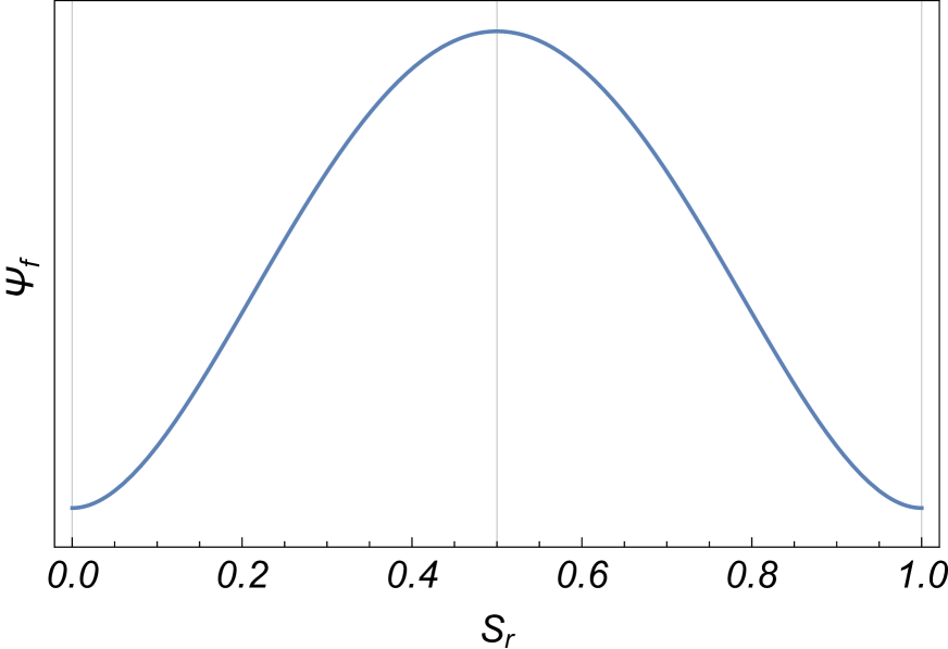
(a) Van der Waals’ like potential

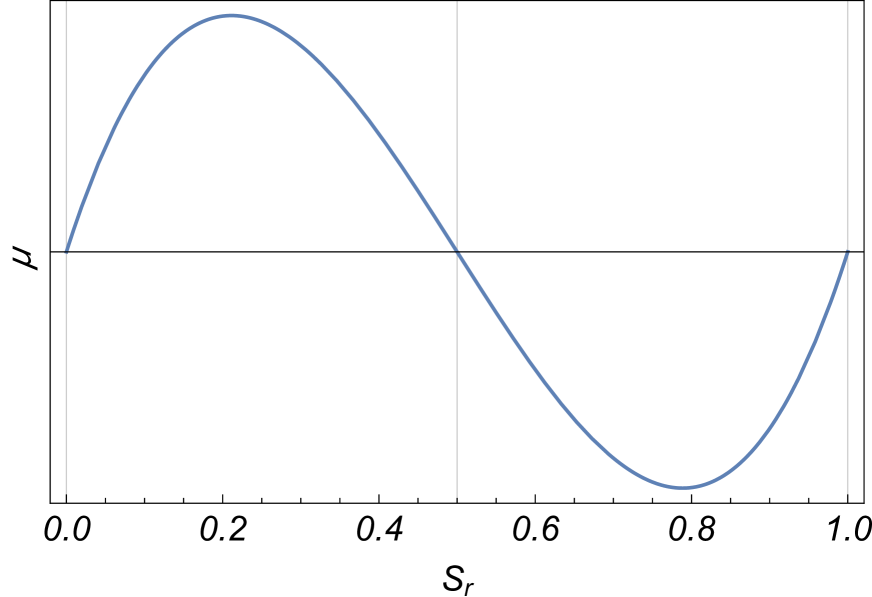
(b) Chemical potential

Figure 1: The liquid and the gaseous phase coexist at equilibrium as they are isopotential minima of the fluid free energy

The non-local contribution allows for governing the coarsening of the domains occupied by the fluid phases and pattern formation. Indeed it provides just a correction of the bulk energy, when considering the so-called flat interface limit, see [16], whilst it constitutes the main part of the energy of the non-uniform fluid, when describing phenomena in which a clear scale separation can not be assumed, as in topological transitions in multi-phase fluids [71] or gravity driven fingering through porous media [33].

Because of the constitutive law (13), the following prescriptions on the fluid stress and hyper-stress hold true

$$\begin{array}[]{ll}\left\{\begin{array}[]{l}p^{f}=-\left[n\,\dfrac{\partial e_{f}}{\partial(1/\rho_{f})}+\kappa_{f}-2\left(1+\dfrac{1}{\mathrm{tr}I}\right)\dfrac{\partial\kappa_{f}}{\partial f_{\rho_{f}}}f_{\rho_{f}}\right],\vskip 6.0pt plus 2.0pt minus 2.0pt\\ \Sigma^{\prime f}_{\alpha\beta}=-2\,\dfrac{\partial\kappa_{f}}{\partial f_{\rho_{f}}}\left[\left(n\rho_{f}\right)_{,\alpha}\left(n\rho_{f}\right)_{,\beta}-\dfrac{1}{\mathrm{tr}I}\left(n\rho_{f}\right)_{,\gamma}\left(n\rho_{f}\right)_{,\gamma}\delta_{\alpha\beta}\right],\end{array}\right.&\pi^{f}_{\alpha}=-2\,\dfrac{\partial\kappa_{f}}{\partial f_{\rho_{f}}}n\rho_{f}\left(n\rho_{f}\right)_{,\alpha},\end{array}$$ (15)

$I$ being the identity tensor and $\mathrm{tr}I=n$ the dimension of the Euclidean space $\mathtt{I}\!\mathtt{E}$. The thermodynamic pressure $\mathcal{P}$ and the chemical potential $\mu$ given in (14) are just a part of these constitutive prescriptions. $\Sigma^{\prime f}$ represents the deviatoric stress acting on the fluid, which is non-vanishing because of the gradient contribution to energy.

As already noticed incompressibility of the liquid phase means that the variations of the density $\rho_{f}$ are univocally determined by the variations of the degree of saturation, so that equation (15) can be rephrased in terms of the saturation ratio $S_{r}$, see e.g. [35]. In particular the double well shape of the energy potential can be prescribed assuming the fluid energy per unit volume of the porous medium to be a kind of Duffing potential

$$\Psi_{f}:=\rho_{f}e_{f}=\mathrm{C}\,\dfrac{\gamma_{nw}}{R}S_{r}^{2}\left(1-S_{r}\right)^{2},$$ (16)

whilst the non-local term is typically assumed quadratic in the gradient of $nS_{r}$:

$$\kappa_{f}\left(f_{\rho_{f}}\right)=\dfrac{\mathrm{C}_{\kappa}}{2}\,(nS_{r})_{,\alpha}(nS_{r})_{,\beta}\,\delta_{\alpha\beta}.$$ (17)

Here $\gamma_{nw}$ is the surface tension between the non-wetting and the wetting phase, whilst $R$ is the characteristic size of the channel through which the fluid can pass, see e.g. [11]. In Figure 1 the energy per unit volume and the corresponding chemical potential are plotted. The energy of the non-uniform fluid could also be prescribed in terms of a different phase field as for instance the mass concentration of the liquid without its double well feature being modified. With an abuse of notation from now on $\mu$ will indicate the derivative of $\Psi_{f}$ with respect to $S_{r}$ rather than to $\rho_{f}$, as indicated in equation (14).

As saturation can not overwhelm the limit $S_{r}=1$, a suitable constraint should be stated when formulating the minimization of the fluid energy potential $\Psi_{f}$ with respect to $S_{r}$, say $S_{r}\leq 1$ which corresponds to $S_{r}-1=-\alpha^{2}$, with $\alpha\geq 0$ a slack variable used to transform the inequality constraint into equality. This yields the introduction of a Lagrangian multiplier, in the functional to be made stationary, representing the reactive chemical potential, $\mu^{\mathrm{r}}$, which allows to account for the transition from partially-saturated to fully-saturated conditions. In partially-saturated states $S_{r}<1$ implies $\alpha\neq 0$ and consequently $\mu^{\mathrm{r}}=0$; on the other hand when saturation is attained $\alpha$ vanishes and the reactive chemical potential plays the role of the liquid pressure in standard saturated poromechanics. Looking at equation (17) it is worth to notice that in the case of saturation the non-local contribution to energy still does not vanish, but reduces to a function of the porosity gradient.

The effect of confinement of the air-water mixture into the porous space, say the retention characteristics of the porous material, will be accounted for by an additional energy $\mathcal{E}_{sf}$. Within the considered framework, no a-priori constitutive characterization is assumed on this functional, but suitable restrictions on it are deduced from the first and the second principle of thermodynamics, summarized in the generalized form of the Clausius-Duhem (dissipation) inequality.

In the following paragraphs the explicit form of the dissipation relative to the partially saturated porous medium is stated, taking in due account the expression of the strain working given by equation (12). The corresponding restrictions on the constitutive law of the porous skeleton and the local diffusion fluid mass flux $M_{k}$ are deduced.

3.1 The first principle of thermodynamics

Modifying the form of the energy equation, stated by [29, equation (3.14)] for a standard porous continuum, so as to separate the interaction energy between the solid and the non-uniform fluid implies the first principle of thermodynamics to read as

$$\dfrac{d_{s}}{dt}\displaystyle\int_{\mathcal{D}}\left(\mathcal{E}_{s}+\dfrac{1}{2}\mathcal{E}_{sf}\right)+\dfrac{d_{f}}{dt}\displaystyle\int_{\mathcal{D}}\left(\mathcal{E}_{f}+\dfrac{1}{2}\mathcal{E}_{sf}\right)=W^{\mathrm{in}}+\mathring{\mathbb{Q}}.$$ (18)

where $d_{c}/dt$ indicates the time derivative following the motion of the particle $c=\{s,f\}$. In a similar way to the fluid, the energy of the solid is defined in terms of the corresponding intrinsic energy as $\mathcal{E}_{s}=(1-n)\rho_{s}e_{s}$. Moreover the rate of change of the coupling energy $\mathcal{E}_{sf}$ is associated partly to the motion of the solid grains, partly to the motion of the molecules of the fluid, say the liquid and the gas. $\mathring{\mathbb{Q}}$ accounts for the rate of heat externally supplied and can be prescribed in terms of a surface rate of heat due to conduction,

$$\mathring{\mathbb{Q}}=-\displaystyle\int_{\partial\mathcal{D}}q_{\alpha}m_{\alpha}=-\displaystyle\int_{\partial\mathcal{D}_{0}}\mathfrak{q_{i}}\,m^{0}_{i}=-\displaystyle\int_{\mathcal{D}_{0}}\mathfrak{q}_{i,i};\quad\mathfrak{q}_{i}:=J\left(F^{-1}\right)_{i\alpha}q_{\alpha},$$ (19)

finally $W^{\textrm{in}}$ is the strain working, given by equation (12). The pull-back of the energy balance (18) into the reference configuration of the skeleton yields

$$\int_{\mathcal{D}_{0}}\left\{\dfrac{d\,\mathbb{E}}{dt}+\left[\dfrac{1}{\rho_{f}n}\left(\mathcal{E}_{f}+\dfrac{1}{2}\mathcal{E}_{sf}\right)M_{k}+\mathfrak{q}_{k}\right]_{,k}\right\}=W^{\mathrm{in}}$$ (20)

where $\mathbb{E}:=J\left(\mathcal{E}_{s}+\mathcal{E}_{f}+\mathcal{E}_{sf}\right)$ is the overall Lagrangian density of internal energy; $d/dt$ indicates the time derivative following the motion of the solid particle fixed in the reference configuration of the skeleton. Equations (12) and (20) imply the following Lagrangian local energy equation to hold true:

$$\begin{array}[]{rl}\dfrac{d\,\mathbb{E}}{dt}=&S_{ij}\dot{E}_{ij}+P_{ijk}\dot{E}_{ij,k}-\left(Jp^{f}\dfrac{M_{k}}{m_{f}}\right)_{,k}-\left[\gamma_{l,l}\dfrac{M_{k}}{m_{f}}-\dfrac{\gamma_{k}}{J}\left(J\dfrac{M_{l}}{m_{f}}\right)_{,l}\right]_{,k}+b^{0f}_{k}\dfrac{M_{k}}{m_{f}}\vskip 6.0pt plus 2.0pt minus 2.0pt\\ &+\left[J\left(F^{-1}\right)_{k\beta}\Sigma^{\prime f}_{\alpha\beta}F_{\alpha q}\,\dfrac{M_{q}}{m_{f}}\right]_{,k}-\left[\dfrac{1}{\rho_{f}n}\left(\mathcal{E}_{f}+\dfrac{1}{2}\mathcal{E}_{sf}\right)M_{k}+\mathfrak{q}_{k}\right]_{,k}.\end{array}$$ (21)

3.2 The second principle of thermodynamics & the Causius-Duhem inequality

In the same way as the first principle, the second principle of thermodynamics (entropy balance) for the porous continuum is stated in the form:

$$\dfrac{d_{s}}{dt}\displaystyle\int_{\mathcal{D}}\rho_{s}(1-n)s_{s}+\dfrac{d_{f}}{dt}\displaystyle\int_{\mathcal{D}}\rho_{f}ns_{f}\geq\displaystyle\int_{\partial\mathcal{D}}\dfrac{q_{\alpha}m_{\alpha}}{T},$$ (22)

where $s_{c}$ stands for the specific entropy of the $c$-th constituent and $q_{\alpha}$ again indicates the surface rate of heat due to conduction. The pull-back of the entropy balance in the reference configuration of the skeleton reads therefore:

$$\int_{\mathcal{D}_{0}}\left[\dfrac{d\,\mathbb{S}}{dt}+\left(s_{f}M_{k}+\dfrac{\mathfrak{q}_{k}}{T}\right)_{,k}\right]\geq 0,$$ (23)

$\mathbb{S}:=J\left(\rho_{s}(1-n)s_{s}+\rho_{f}ns_{f}\right)$ being the overall Lagrangian entropy. Using the Legendre transform $\Psi=\mathbb{E}-T\,\mathbb{S}$; the local form of equation (23) can be written as:

$$\dfrac{d\,\mathbb{E}}{dt}-\mathbb{S}\dfrac{dT}{dt}-\dfrac{d\Psi}{dt}\geq-T\left(s_{f}M_{k}+\dfrac{\mathfrak{q}_{k}}{T}\right)_{,k};$$ (24)

which using equation (21) delivers the Clausius-Duhem inequality for a porous material within the framework of gradient poromechanics, see [88] for similar results:

$$\begin{array}[]{l}S_{ij}\dot{E}_{ij}+P_{ijk}\dot{E}_{ij,k}-\left(Jp^{f}\dfrac{M_{k}}{m_{f}}\right)_{,k}-\left[\gamma_{l,l}\dfrac{M_{k}}{m_{f}}-\dfrac{\gamma_{k}}{J}\left(J\dfrac{M_{l}}{m_{f}}\right)_{,l}\right]_{,k}+\left[J\left(F^{-1}\right)_{k\beta}\Sigma^{\prime f}_{\alpha\beta}F_{\alpha q}\,\dfrac{M_{q}}{m_{f}}\right]_{,k}\vskip 6.0pt plus 2.0pt minus 2.0pt\\ +\,b^{0f}_{k}\dfrac{M_{k}}{m_{f}}-\left[\dfrac{1}{\rho_{f}n}\left(\mathcal{E}_{f}+\dfrac{1}{2}\mathcal{E}_{sf}\right)M_{k}+\mathfrak{q}_{k}\right]_{,k}+T\left(s_{f}M_{k}+\dfrac{\mathfrak{q}_{k}}{T}\right)_{,k}-\mathbb{S}\,\dfrac{dT}{dt}-\dfrac{d\Psi}{dt}\geq 0.\end{array}$$ (25)

3.3 Dissipation

A characterization of the dissipation relative to the solid and the non-uniform fluid is obtained, starting from the Clausius-Duhem inequality (25), separating, within the overall free energy $\Psi$ and the overall entropy $\mathbb{S}$, the contributions of the bulk fluid, say $m_{f}\psi_{f}$ and $m_{f}s_{f}$, from the residual terms relative to the energy and the entropy of the bulk skeleton and the interfaces, say $\Psi_{s}$ and $\mathbb{S}_{s}$:

$$\Psi_{s}=\Psi-m_{f}\,\psi_{f}\left(\rho_{f},T\right),\quad\mathbb{S}_{s}=\mathbb{S}-m_{f}s_{f}.$$ (26)

Remind that $\psi_{f}=e_{f}-T\,s_{f}$ is the Legendre transformation of $e_{f}$, such that $\partial\psi_{f}/\partial T=-s_{f}$. This approach stems from [7], who defined the wetted solid as a system composed of the solid skeleton and a thin layer of fluid attached to the internal walls of the pore. The aim is proving that $\Psi_{s}$ is a state function which prescribes the constitutive behavior of the skeleton in thermo-poroelasticity, say in the case when just reversible processes are involved by the deformation of the porous continuum. In this case the residual part of the dissipation will depend just on the Lagrangian filtration vector $M_{k}$ and the gradient of the absolute temperature.

The fluid mass conservation (2) together with the constitutive law relative to the fluid stress and hyper-stress (15), allow to rephrase the Clausius-Duhem inequality (25) in the following form:

$$\begin{array}[]{l}\Phi:=S_{ij}\dot{E}_{ij}+P_{ijk}\dot{E}_{ij,k}+\left(\mathcal{P}+\dfrac{1}{2n}\,\mathcal{E}_{sf}+\dfrac{\gamma_{k}}{\phi}\,\dfrac{J_{,k}}{J}\right)\dfrac{d\phi}{dt}+\dfrac{\phi}{S_{r}}\left(\dfrac{1}{2n}\,\mathcal{E}_{sf}+\dfrac{\gamma_{k}}{\phi}\,\dfrac{J_{,k}}{J}\right)\dfrac{dS_{r}}{dt}-\left(\dfrac{\gamma_{k}}{\phi S_{r}}\right)\dfrac{d(\phi S_{r})_{,k}}{dt}\vskip 6.0pt plus 2.0pt minus 2.0pt\\ -\mathbb{S}_{s}\dfrac{dT}{dt}-\dfrac{d\Psi_{s}}{dt}-\dfrac{1}{\rho_{L}}\left\{\dfrac{1}{S_{r}}\mathcal{P}_{,k}+\left[\left(\dfrac{\gamma_{l}}{\phi S_{r}}\right)_{,l}+\dfrac{1}{S_{r}}\left(\dfrac{1}{2n}\mathcal{E}_{sf}+\dfrac{\gamma_{l}}{\phi}\dfrac{J_{,l}}{J}\right)\right]_{,k}-\dfrac{b_{k}^{0f}}{\phi S_{r}}\right\}M_{k}-\dfrac{\mathfrak{q}_{k}}{T}T_{,k}\geq 0.\end{array}$$ (27)

The coefficients of $d\phi/dt$, $dS_{r}/dt$, $d\left(\phi S_{r}\right)_{,k}/dt$ and $M_{k}$ reported in equation (27) are explicitly deduced from equation (25) in Appendix A. Following [29] the dissipation (27) can be split into three terms, one related to the solid skeleton, one to the non-uniform fluid and the last one referred to thermal effects. These three contributions are separately assumed non-negative:

$$\Phi_{s}= S_{ij}\dot{E}_{ij}+P_{ijk}\dot{E}_{ij,k}+\mathcal{P}\dfrac{d\phi}{dt}+\dfrac{1}{S_{r}}\left(\dfrac{\mathcal{E}_{sf}}{2n}+\dfrac{\gamma_{k}}{\phi}\,\dfrac{J_{,k}}{J}\right)\dfrac{d(\phi S_{r})}{dt}-\dfrac{\gamma_{k}}{\phi S_{r}}\dfrac{d(\phi S_{r})_{,k}}{dt}-\mathbb{S}_{s}\dfrac{dT}{dt}-\dfrac{d\Psi_{s}}{dt}\geq 0,$$ (28)

$$\Phi_{f}= -\dfrac{1}{\rho_{L}}\left\{\dfrac{1}{S_{r}}\mathcal{P}_{,k}+\left[\left(\dfrac{\gamma_{l}}{\phi S_{r}}\right)_{,l}+\dfrac{1}{S_{r}}\left(\dfrac{1}{2n}\mathcal{E}_{sf}+\dfrac{\gamma_{l}}{\phi}\dfrac{J_{,l}}{J}\right)\right]_{,k}-\dfrac{b_{k}^{0f}}{\phi S_{r}}\right\}M_{k}\geq 0,$$ (29)

$$\Phi_{th}= -\dfrac{\mathfrak{q}_{k}}{T}T_{,k}\geq 0.$$ (30)

As previously remarked, equation (28) states that within thermo-poroelasticity the Helmholtz free energy of the skeleton is a state function:

$$\Psi_{s}=\widehat{\Psi}_{s}(E_{ij},E_{ij,k},\phi,S_{r},(\phi S_{r})_{,k},T),$$ (31)

which depends not only on the strain of the skeleton, the Lagrangian porosity and the degree of saturation, as in standard unsaturated poromechanics, but also on the gradient of strain, $E_{ij,k}$, and the gradient of Lagrangian water content, $(\phi S_{r})_{,k}$. It is worth to notice that equation (31) could be also formulated considering a free energy function depending on the gradient of strain, $E_{ij,k}$, and the gradient of water content, $(nS_{r})_{,k}$, in addition to the dependence on $(E_{ij},\phi,S_{r})$, so modifying the definition of conjugate variables.

As the fluid dissipation (29) does not vanish except at equilibrium, the filtration force must be related to the filtration vector itself, in a way to fulfill the dissipation inequality during evolution. Finally equation (30) recalls the well-known result that heat flows through materials along the direction of the negative gradient of temperature (from higher to lower).

Now, assuming isothermal conditions, the poro-elastic constitutive equations of the solid skeleton and the generalized Darcy law relative to the fluid are deduced and compared with those ones typically adopted in modeling the behavior of partially saturated porous media.

4 Poroelastic constitutive relations

According with equation (28) and its corollary remarks, the poroelastic constitutive relations of the solid skeleton must fulfill the following restriction:

$$\begin{array}[]{l}\left(S_{ij}-\dfrac{\partial\Psi_{s}}{\partial E_{ij}}\right)\dfrac{dE_{ij}}{dt}+\left(P_{ijk}-\dfrac{\partial\Psi_{s}}{\partial E_{ij,k}}\right)\dfrac{dE_{ij,k}}{dt}+\left[\mathcal{P}+\left(\dfrac{1}{2n}\mathcal{E}_{sf}+\dfrac{\gamma_{k}}{\phi}\,\dfrac{J_{,k}}{J}\right)-\dfrac{\partial\Psi_{s}}{\partial\phi}\right]\dfrac{d\phi}{dt}\,+\vskip 6.0pt plus 2.0pt minus 2.0pt\\ \left[\dfrac{\phi}{S_{r}}\left(\dfrac{1}{2n}\mathcal{E}_{sf}+\dfrac{\gamma_{k}}{\phi}\,\dfrac{J_{,k}}{J}\right)-\dfrac{\partial\Psi_{s}}{\partial S_{r}}\right]\dfrac{dS_{r}}{dt}+\left(-\dfrac{\gamma_{k}}{\phi S_{r}}-\dfrac{\partial\Psi_{s}}{\partial(\phi S_{r})_{,k}}\right)\dfrac{d(\phi S_{r})_{,k}}{dt}=0,\end{array}$$ (32)

if no frozen contribution to the free energy has been taken into account, see e.g. [27] and [32]. Within this framework one gets the constitutive relations for the overall stresses $S_{ij}$ and $P_{ijk}$,

$$S_{ij}=\dfrac{\partial\Psi_{s}}{\partial E_{ij}},\qquad P_{ijk}=\dfrac{\partial\Psi_{s}}{\partial E_{ij,k}},$$ (33)

the constitutive prescription for the coupling energy term $\mathcal{E}_{sf}$,

$$\dfrac{\phi}{S_{r}}\left(\dfrac{1}{2n}\mathcal{E}_{sf}+\dfrac{\gamma_{k}}{\phi}\dfrac{J_{,k}}{J}\right)=\dfrac{\partial\Psi_{s}}{\partial S_{r}},$$ (34)

and the constitutive constraints to be satisfied by the skeleton free energy once the thermodynamic pressure $\mathcal{P}$ and the fluid hyper-stress $\gamma_{k}$ have been assigned according with equation (16), say

$$\mathcal{P}+\left(\dfrac{1}{2n}\mathcal{E}_{sf}+\dfrac{\gamma_{k}}{\phi}\dfrac{J_{,k}}{J}\right)=\dfrac{\partial\Psi_{s}}{\partial\phi},\qquad\dfrac{\gamma_{k}}{\phi S_{r}}=-\dfrac{\partial\Psi_{s}}{\partial(\phi S_{r})_{,k}}.$$ (35)

When the gradient contribution to the fluid energy vanishes, equation (34) reduces to the prescription of the macro-scale capillary pressure, postulated in classical unsaturated poromechanics, see [29], say $\phi\mathcal{P}_{c}=-\partial\Psi_{s}/\partial S_{r}$, if one assumes

$$\mathcal{P}_{c}:=-\dfrac{1}{S_{r}}\left(\dfrac{1}{2n}\mathcal{E}_{sf}\right).$$ (36)

As a consequence equations (34) and (35)₁ can be rephrased as the generalized constitutive characterizations of the macro-scale capillary pressure $\mathcal{P}_{c}$ and the fluid thermodynamic pressure $\mathcal{P}$, which account for the spatial distribution of interfaces, within the porous network, considering the additional contribution of the fluid hyper-stress:

$$\phi\mathcal{P}_{c}=-\dfrac{\partial\Psi_{s}}{\partial S_{r}}+\dfrac{\gamma_{k}}{S_{r}}\,\dfrac{J_{,k}}{J},\qquad\mathcal{P}-S_{r}\mathcal{P}_{c}+\dfrac{\gamma_{k}}{\phi}\,\dfrac{J_{,k}}{J}=\dfrac{\partial\Psi_{s}}{\partial\phi}.$$ (37)

Equation (33) is standard, within the framework of gradient theories of continuum mechanics; on the other hand equations (37) deserve a deeper discussion in order to understand in which sense they can be considered an enhanced constitutive prescription of the macro-scale capillary pressure and the thermodynamic pressure of the fluid. Developing a micro-scale analysis this model will be compared, in § 6, with the micro-structured one which accounts for the dependence of the capillary pressure on the so-called interfacial area between the non-wetting and the wetting phase, see e.g. [58, 59, 64, 81].

4.1 Generalized effective stresses

Some additional remarks can be deduced from the thermodynamical restrictions stated by equation (28) if the solid grains, which constitute the matrix of the porous medium, undergo negligible volume change. In this case the Lagrangian porosity is definitely prescribed in terms of volume changes of the porous elementary volume, say: $J=1+\phi-\phi_{0}$, $\phi_{0}$ being the reference value of porosity, see e.g. [29, Chapter 3]. The solid dissipation can therefore be rewritten and the generalization of Bishop’s effective stress naturally arises, within the framework of the considered gradient model. Assuming small strains, but allowing the porous skeleton to suffer strain gradients of order $O(1)$, with respect to the considered small perturbation parameter, the simplified expression of $\Phi_{s}$ reads as follows:

$$\Phi_{s}=S^{\prime}_{ij}\dot{E}_{ij}+P^{\prime}_{ijk}\dot{E}_{ij,k}-\phi\mathcal{P}_{c}\,\dot{S}_{r}-\dfrac{\gamma_{k}}{\phi S_{r}}\,\dfrac{d(nS_{r})_{,k}}{dt}-\dot{\Psi}_{s}.$$ (38)

Here $S^{\prime}_{ij}$ and $P^{\prime}_{ijk}$ are the generalized Bishop stress and hyper-stress defined by

$$S^{\prime}_{ij}:=S_{ij}+\left(\mathcal{P}-S_{r}\mathcal{P}_{c}\right)\delta_{ij}+\gamma_{k}\left(2E_{ij,k}-\delta_{ij}\dfrac{(nS_{r})_{,k}}{\phi S_{r}}\right),\qquad P^{\prime}_{ijk}:=P_{ijk}-\gamma_{k}\delta_{ij}.$$ (39)

As a consequence the corresponding free energy of the solid skeleton can be regarded as a state function of strain, strain gradient, saturation degree and gradient of liquid content, only. The general form of equations (39), when no restriction to small strains is assumed, is reported in Appendix B.

If one aims at investigating non-reversible processes affecting the behavior of the solid skeleton, different dissipative mechanisms should be analyzed, which could concern interactions among the grains of the solid skeleton, or between the grains and the fluid. In the first case inelastic constitutive relations for the solid stress and (eventually) hyper-stress should be introduced, in the second one hysteresis during wetting-drying cycles should modify the prescriptions of the retention properties, see e.g. [60]. It is not the goal of this paper to address modeling inelastic processes, however this can be done specifying the way in which dissipation depends on a suitable set of internal variables.

4.2 Generalized Darcy law

As usual in poromechanics the dissipation inequality (29) relative to the fluid can be satisfied requiring $\Phi_{f}$ to be a quadratic function of $M_{k}$, which means: $\Phi_{f}=\left(A_{kl}M_{l}M_{k}\right)/\rho^{2}_{L}.$ This implies the coefficient of $M_{k}$ in equation (29) to be constitutively constrained to

$$-\dfrac{1}{S_{r}}\mathcal{P}_{,k}-\left[\left(\dfrac{\gamma_{l}}{\phi S_{r}}\right)_{,l}+\dfrac{1}{S_{r}}\left(\dfrac{1}{2n}\mathcal{E}_{sf}+\dfrac{\gamma_{l}}{\phi}\dfrac{J_{,l}}{J}\right)\right]_{,k}+\dfrac{b_{k}^{0f}}{\phi S_{r}}=\dfrac{1}{\rho_{L}}A_{kl}M_{l},$$ (40)

which reads as a generalization of classical Darcy’s law. $A_{kl}$ is the inverse of permeability, its dimension is therefore $\left[A\right]=L^{-3}\,M\,T^{-1}$. According to equations (14) and (37) equation (40) can be reformulated as follows

$$-\left[\dfrac{\partial\left(S_{r}\,\rho_{L}e_{f}\right)}{\partial S_{r}}-\left(\dfrac{\partial\Psi_{s}}{\partial(\phi S_{r})_{,l}}\right)_{,l}+\dfrac{\partial U}{\partial S_{r}}\right]_{,k}+\dfrac{b_{k}^{0f}}{\phi S_{r}}=\dfrac{1}{\rho_{L}}A_{kl}M_{l},$$ (41)

where $S_{r}\rho_{L}e_{f}$ is the specific free energy of the fluid per unit volume of the pores and therefore coincides with the double-well energy potential $\Psi_{f}$, possibly describing coexistence of the liquid and the gaseous phases, see equation (16). For the sake of simplicity, the capillary energy $U$ has been introduced, following [31], so that $\partial\Psi_{s}/\partial S_{r}=\phi\,\partial U/\partial S_{r}$.

According with classical arguments proposed within the framework of diffuse interface models in fluid mechanics, see e.g. [62, 63, 12], the first two terms in equation (41) correspond to the so-called generalized chemical potential of the non-uniform fluid defined as

$$\text{\textmu}=\dfrac{\partial\Psi_{f}}{\partial S_{r}}-\left(\dfrac{\partial\Psi_{s}}{\partial\left(\phi S_{r}\right)_{,l}}\right)_{,l},$$ (42)

the whole quantity $\text{\textmu}+\partial U/\partial S_{r}$ can therefore be interpreted as the generalized chemical potential of the pore-fluid, say of the non-uniform fluid within the pore network. This last accounts, on one hand, for surface tension effects which are typical of a diphasic fluid on the other one for the retention properties of the skeleton, due to its texture, by means of $\partial U/\partial S_{r}$.

Apparently the role of the capillary energy $U$ is that of modifying the double-well potential $\Psi_{f}$ which prescribes the free energy of the fluid, in order to account for the presence of a confining surface densely distributed within the porous continuum. The new free energy $\left(\Psi_{f}+U\right)$, which can be called effective energy of the pore-fluid, has not the same minima as $\Psi_{f}$, as they are shifted inward the interval $(0,1)$ from below or from above whether the solid skeleton is gas or liquid wet, see e.g. [79, 80]. In § 5 the effects of combining these two energy contributions are discussed, considering the retention properties of different soils. A similar behavior has been discussed by [36], modeling two-phase flow in a Hele-Shaw cell, introducing a suitable symmetry-breaking function.

5 Constitutive characterization of the pore-fluid

Providing a constitutive characterization of the pore-fluid, say of the fluid within the pore network, is generally achieved, in unsaturated poromechanics, assuming a proper prescription of the retention curve, which means prescribing the capillary pressure $\mathcal{P}_{c}$, or the capillary energy $U$, as a function of $S_{r}$. As already noticed in § 3 however, the air-water mixture, which saturates the pore space, is regarded here as a non-uniform fluid, the corresponding saturation ratio being used to characterize the state of the fluid at any current placement. No distinction is therefore made explicit between the pressure of the liquid and the pressure of the gaseous phase, as well as between the corresponding chemical potentials. Moreover no algebraic relation between the saturation degree and the capillary pressure or the chemical potential of the fluid can a-priori be stated, without solving, at least at equilibrium, the following generalized Richards equation:

$$\dfrac{d(\phi S_{r})}{dt}-\left\{K_{\textrm{sat}}\,k(S_{r})\left[\left(\dfrac{\partial\Psi_{f}}{\partial S_{r}}-\left(\dfrac{\partial\Psi_{s}}{\partial(\phi S_{r})_{,l}}\right)_{,l}+\dfrac{\partial U}{\partial S_{r}}\right)_{,k}-\dfrac{b^{0f}_{k}}{\phi S_{r}}\right]\right\}_{,k}=0.$$ (43)

Here the permeability of the porous medium has been assumed isotropic: $(A^{-1})_{mk}=K_{\textrm{sat}}\,k(S_{r})\delta_{mk}$, $K_{\textrm{sat}}$ being the so-called saturated permeability and $k(S_{r})$ the relative permeability of the wetting phase, see e.g. [29, 30]. As usual in unsaturated poromechanics equation (43) which provides the distribution in space and time of the saturation degree is deduced merging the mass conservation law (2) and the Darcy law, which in this case takes the form given by equation (41).

At stationary conditions, say when $\partial(\phi S_{r})/\partial t=0$, equation (43) reduces to a fourth order partial differential equation in the space variable, which is definitely similar to the one prescribing the mass density distribution of a Cahn-Hilliard fluid at equilibrium. However a fundamental additional term is here accounted for, say the derivative of $U$ with respect to $S_{r}$, which allows for describing the confining effect on the non-uniform fluid, due to the presence of the porous skeleton. Equation (43) looks also similar to that one stated in [37, equation (2)] and [33, equation (13)], who adopted a phase field model for describing gravity fingers and saturation overshoot, during water infiltration through a non-deformable soil. In this case the difference resides in the account for the chemical potential $\mu=\partial\Psi_{f}/\partial S_{r}$ in (43), allowing for possible coexistence between the phases of the non-uniform fluid. Moreover equation (43) is here definitely coupled with the balance equation of the overall continuum.

Following the same procedure which induced the definition of the generalized chemical potential (42) when simulating multi-phase flows, see e.g. [12], equation (43) can be rephrased in terms of the functional derivative of the free energy of the pore-fluid

$$\mathcal{F}[S_{r}]=\displaystyle\int_{\mathcal{D}_{0}}\left[\left(\Psi_{f}(S_{r})+U(S_{r})\right)+\kappa_{f}\,(nS_{r})_{,k}(nS_{r})_{,l}\,\delta_{kl}\right]$$ (44)

with respect to $S_{r}$, as follows:

$$\left\{\begin{array}[]{l}\dfrac{d(\phi S_{r})}{dt}=\left[K_{\textrm{sat}}\,k(S_{r})\left(\text{\textmu}^{\textrm{eff}}_{,k}-\dfrac{b^{0f}_{k}}{\phi S_{r}}\right)\right]_{,k},\vskip 6.0pt plus 2.0pt minus 2.0pt\\ \text{\textmu}^{\textrm{eff}}=\dfrac{\delta\mathcal{F}}{\delta S_{r}}=\dfrac{\partial\Psi_{f}}{\partial S_{r}}-\left(\dfrac{\partial\Psi_{s}}{\partial(\phi S_{r})_{,l}}\right)_{,l}+\dfrac{\partial U}{\partial S_{r}},\end{array}\right.$$ (45)

where the generalized effective chemical potential of the pore-fluid $\text{\textmu}^{\textrm{eff}}$ has been introduced. The energy of the skeleton depends on the gradient of the liquid content, so that the gradient contribution to the constitutive law of the non-uniform fluid is not modified, with respect to equation (15). For the sake of completeness the effective chemical potential of the pore-fluid, accounting only for the derivative of the effective energy $\Psi_{f}+U$ is defined as $\mu^{\textrm{eff}}:=\partial(\Psi_{f}+U)/\partial S_{r}=\mu+\partial U/\partial S_{r}$. As already noticed $\text{\textmu}^{\textrm{eff}}$ is different from µ, because of the term involving the derivative of the capillary energy $U$, but it also differs from the flow potential $\Phi$ introduced by [33, equation (12)], because of the term involving the derivative of the fluid energy $\Psi_{f}$.

The role of $\Psi_{f}$ and $U$ in the characterization of the spatial distribution of $S_{r}$, $\mu$, $\mathcal{P}_{c}$ and $\text{\textmu}^{\textrm{eff}}$ deserves a deeper analysis in order to underline the main differences between the proposed modified Richards equation (45) and that one stated by [33] for describing gravity fingering in soils. In Figure 2 the chemical potential of the pure fluid prescribed, according with equation (16), as

$$\mu=\dfrac{\partial\Psi_{f}}{\partial S_{r}}=(\rho_{L}g)\,h_{f},\qquad h_{f}=2C\dfrac{\gamma_{nw}}{(\rho_{L}g)\,R}\,S_{r}\left(1-3S_{r}+2S_{r}^{2}\right),$$ (46)

and the derivative of the capillary energy, given by a van Genuchten-like curve

$$\dfrac{\partial U}{\partial S_{r}}=-(\rho_{L}g)\,h_{U},\qquad h_{U}=\dfrac{1}{\alpha}\left[\left(\dfrac{S_{r}-S_{r}^{\textrm{res}}}{1-S_{r}^{\textrm{res}}}\right)^{-\frac{1}{m}}-1\right]^{\frac{1}{n}},$$ (47)

are depicted (gray dotted and gray dashed lines, respectively), considering different soil textures and therefore different choices for the relative partition of sand, clay and silt in the soil. The profile of the negative effective chemical potential of the pore-fluid $\mu^{\textrm{eff}}$ with respect to $S_{r}$ is also drawn in each panel of Figure 2 (solid lines). Both the chemical potential and the derivative of th capillary energy are expressed in head units, via the two fields $h_{f}$ and $h_{U}$, adopting the classical [69] scaling, which prescribes the characteristic length $R$ in terms of the intrinsic permeability $\varkappa$ (of the soil): $R=\sqrt{\varkappa/\phi_{0}}$. The different values of the parameters $S^{\mathrm{res}}_{r}$, $\alpha$ and $n$ ($m=1-1/n$), which characterize the retention curve (47) for the considered soil textures, are listed in the panels.

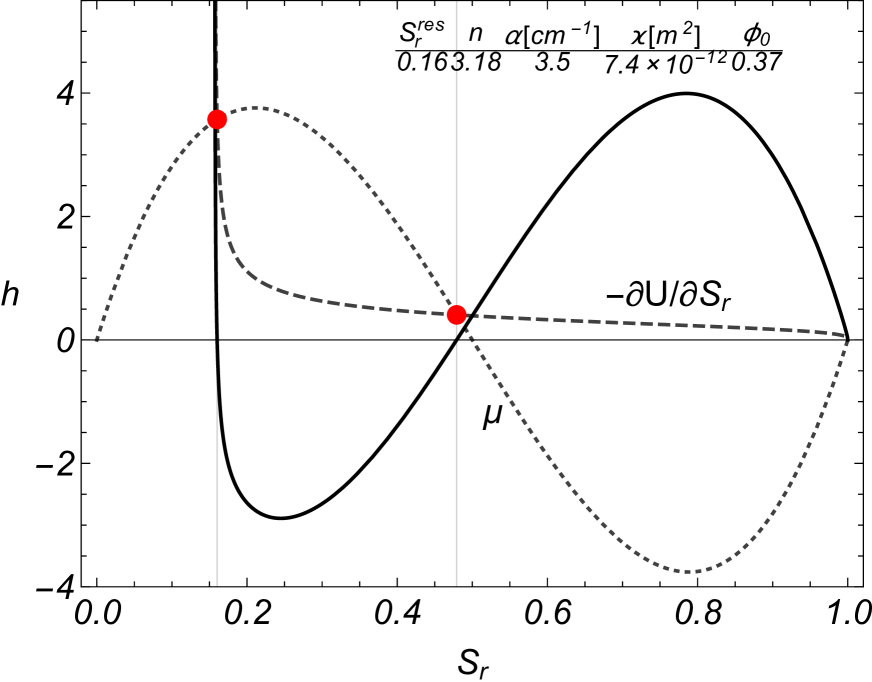
(a) Sand

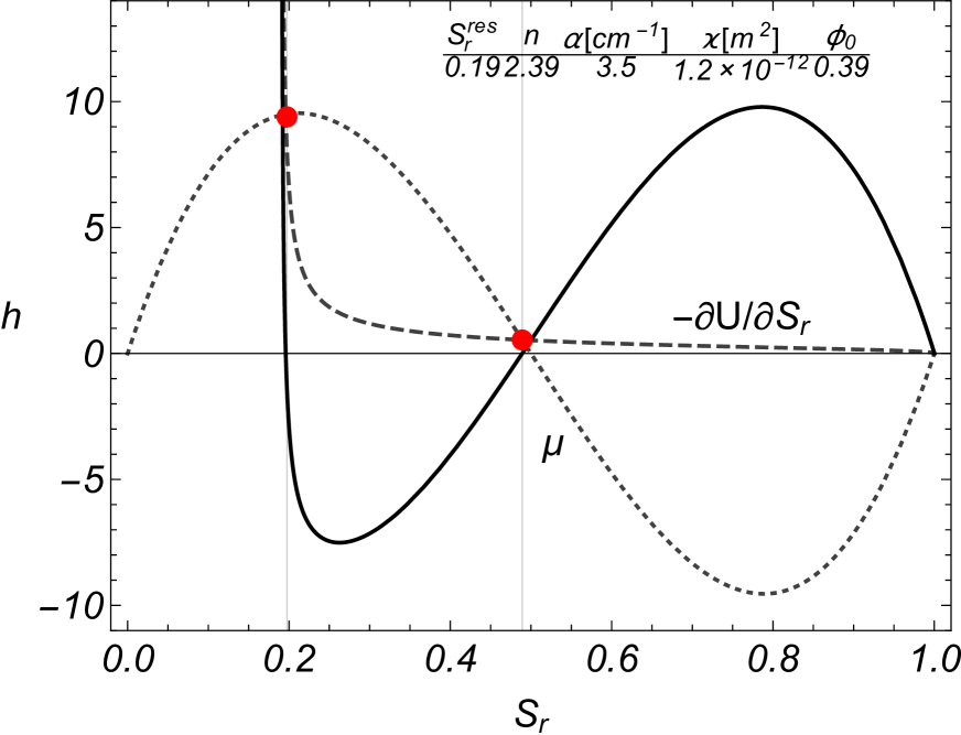
(b) Loamy sand

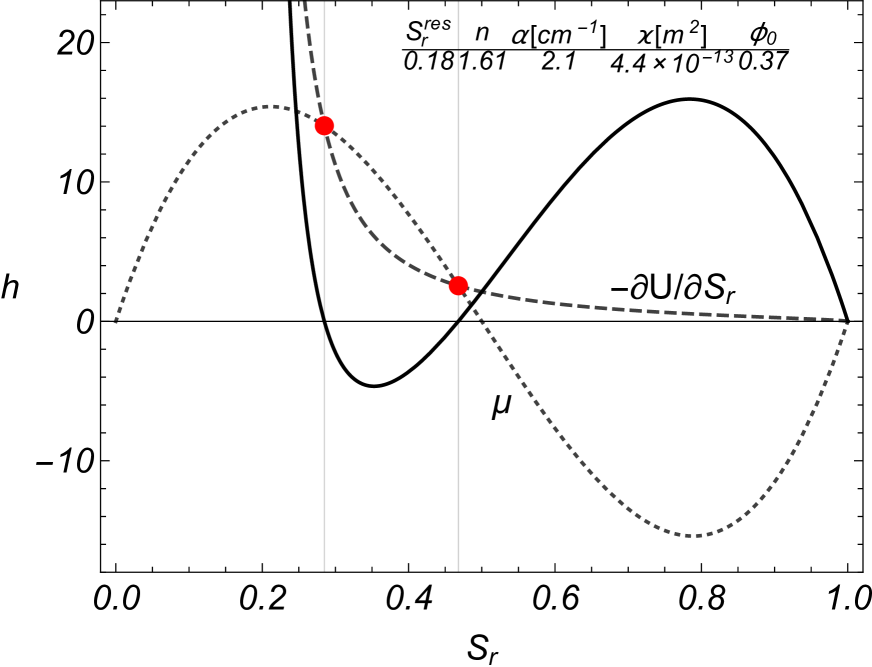
(c) Sandy loam

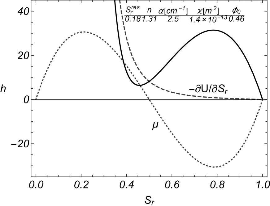
(d) Loam

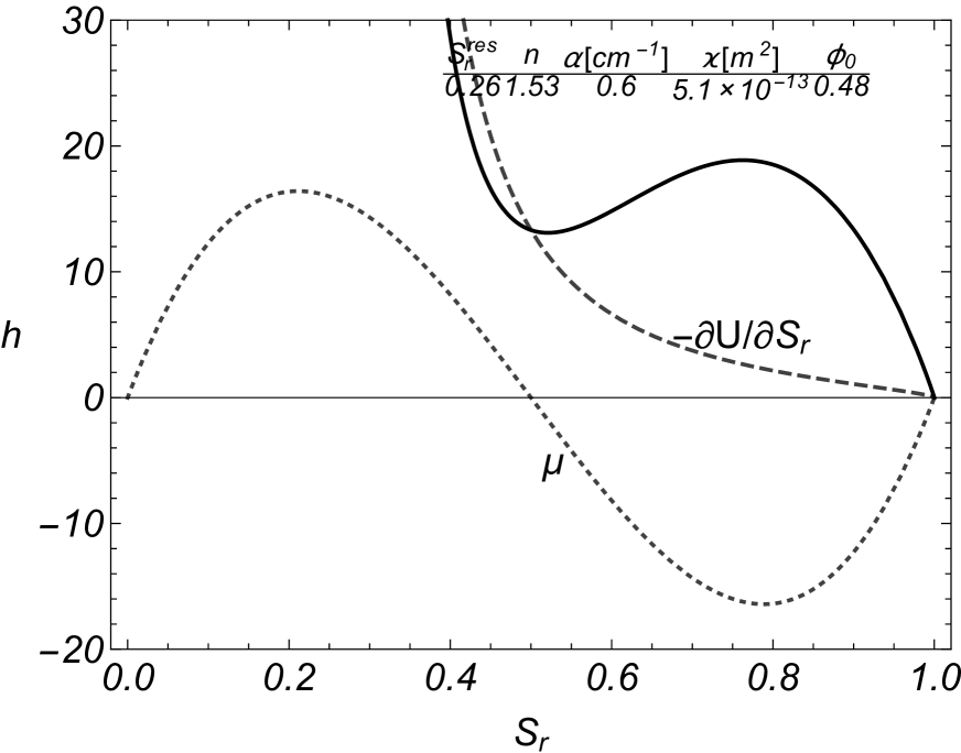
(e) Silt

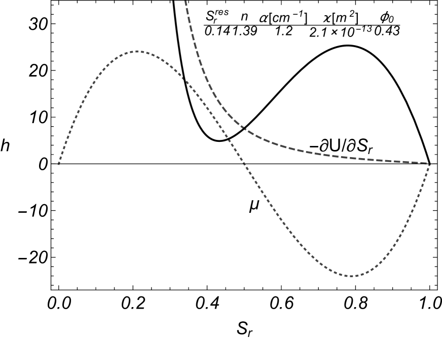
(f) Silt loam

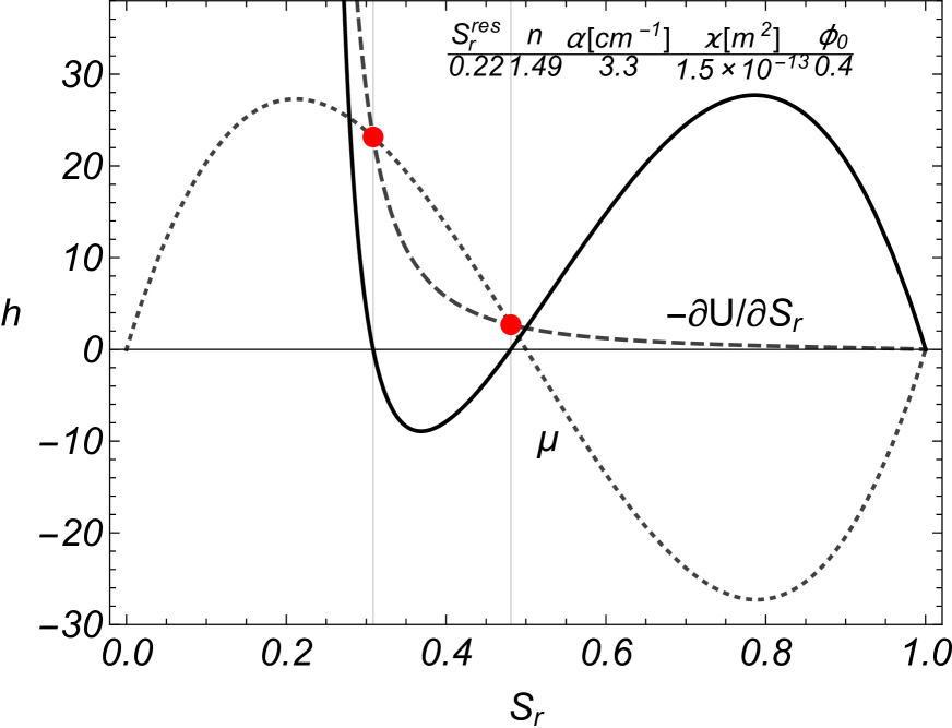
(g) Sandy clay Loam

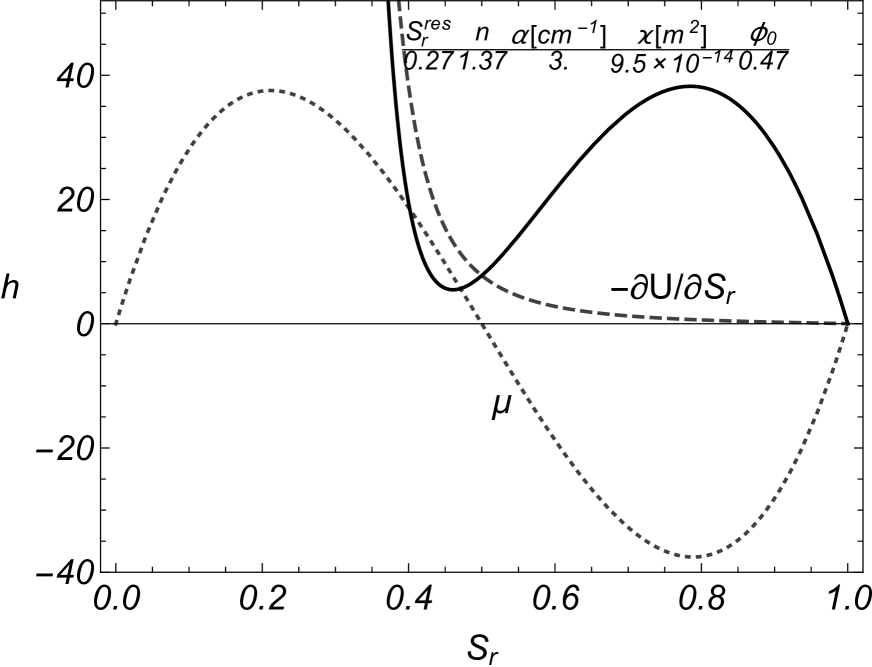
(h) Clay loam

(i) Silty clay loam

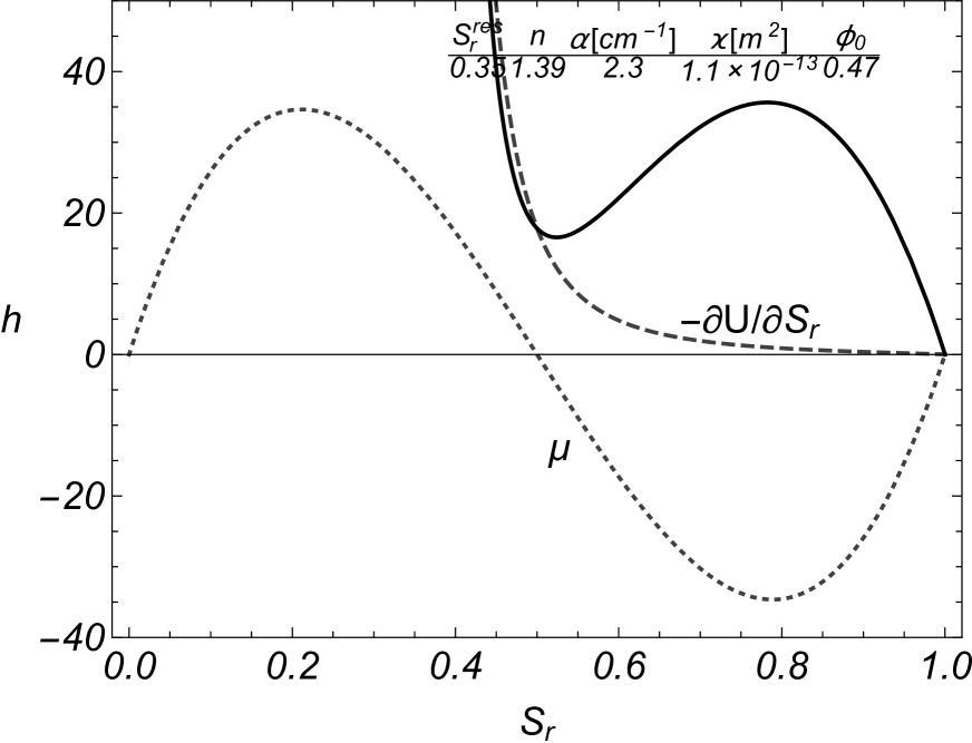
(j) Silty clay

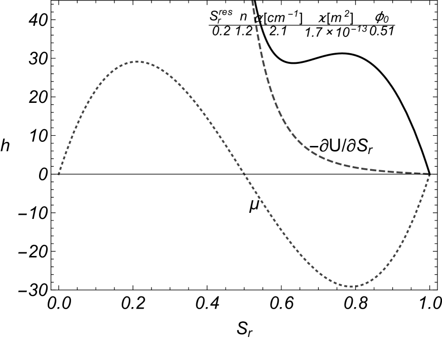
(k) Clay

Figure 2: Heads relative to the chemical potential $\mu$ of the pure fluid (dotted gray line), the derivative of the capillary energy (dashed gray line) and the negative effective chemical potential $\mu^{\textrm{eff}}$ (solid black line). The values of the parameters which characterize the retention curve (47) are listed in each panel, together with the intrinsic permeability $\varkappa$ and the referential porosity $\phi_{0}$, relative to the portion of sand, clay and silt which constitute the soil. The red spots in panels (a), (b), (c), (g) and (i) highlight the real zeros of $\mu+\partial U/\partial S_{r}$, different from $S_{r}=1$, which corresponds to the highest relative minimum and the saddle point of the effective free energy $\Psi_{f}+U$.

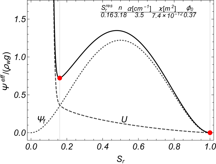
(a) Sand

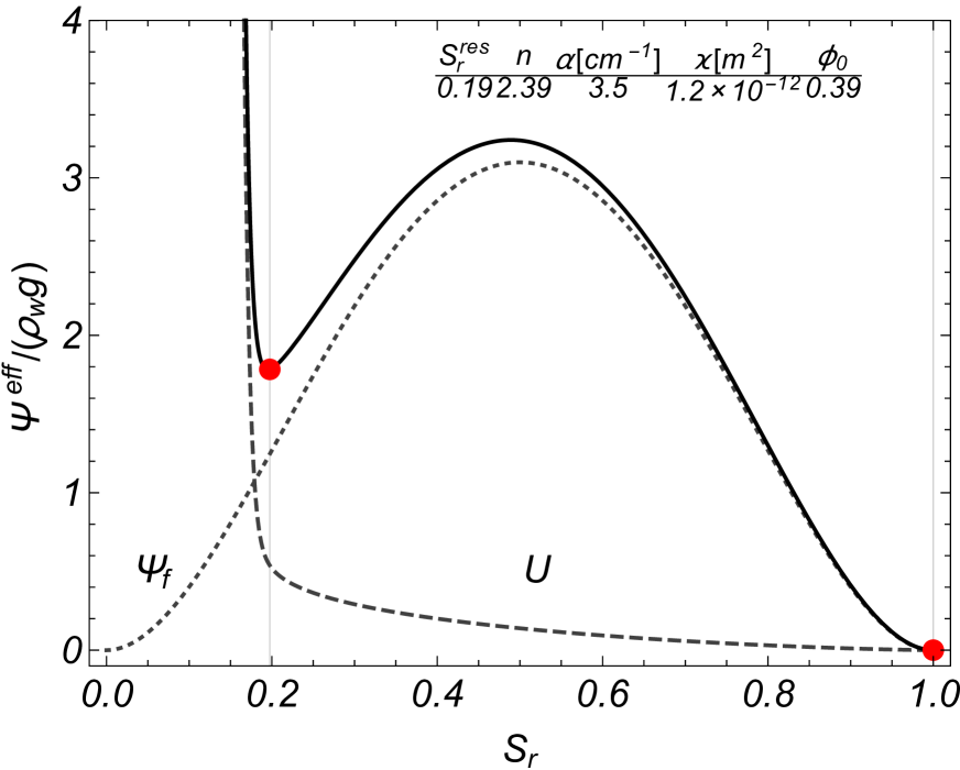
(b) Loamy sand

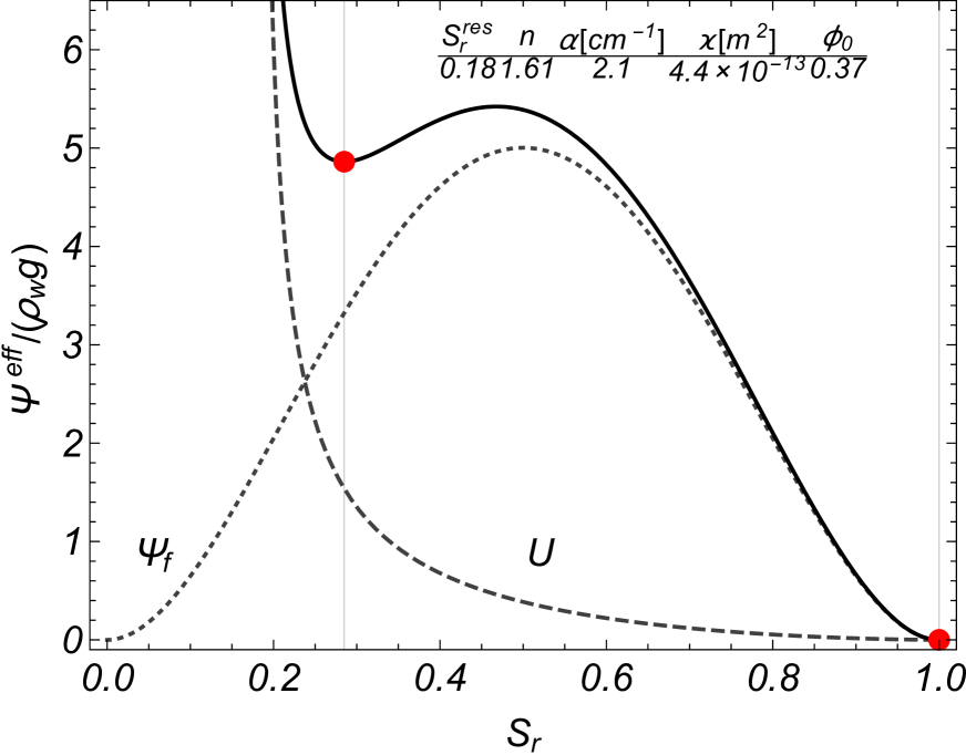
(c) Sandy loam

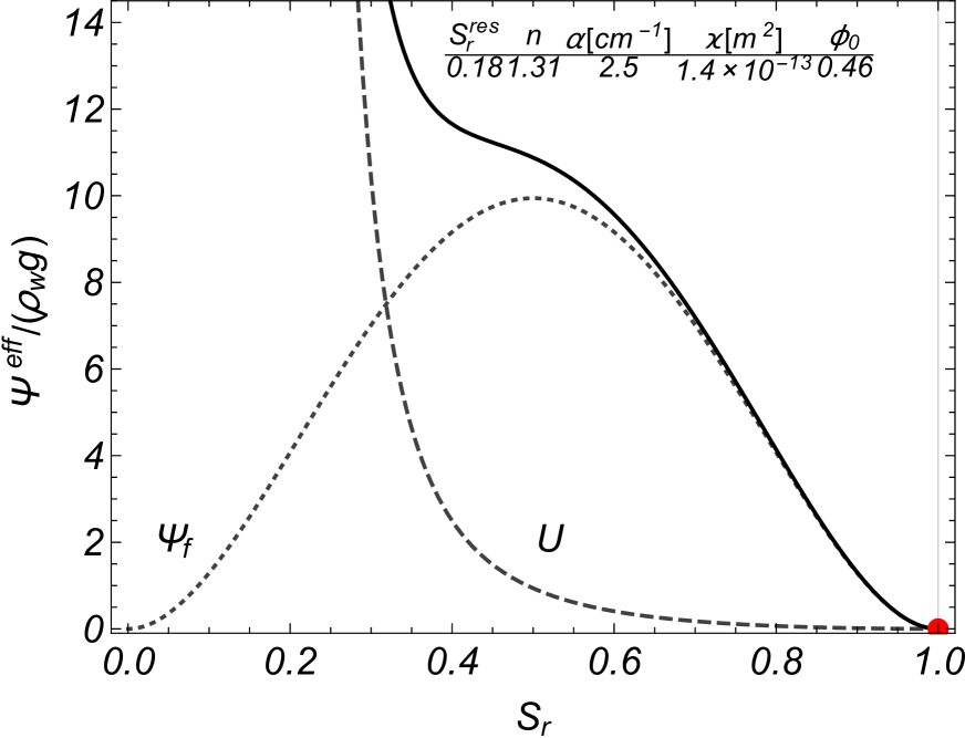
(d) Loam

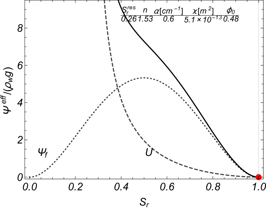
(e) Silt

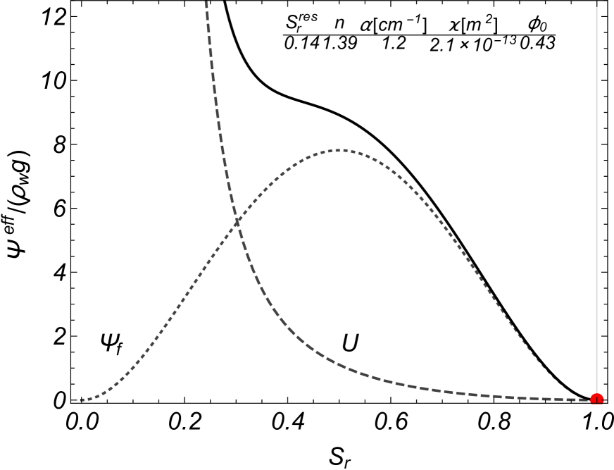
(f) Silt loam

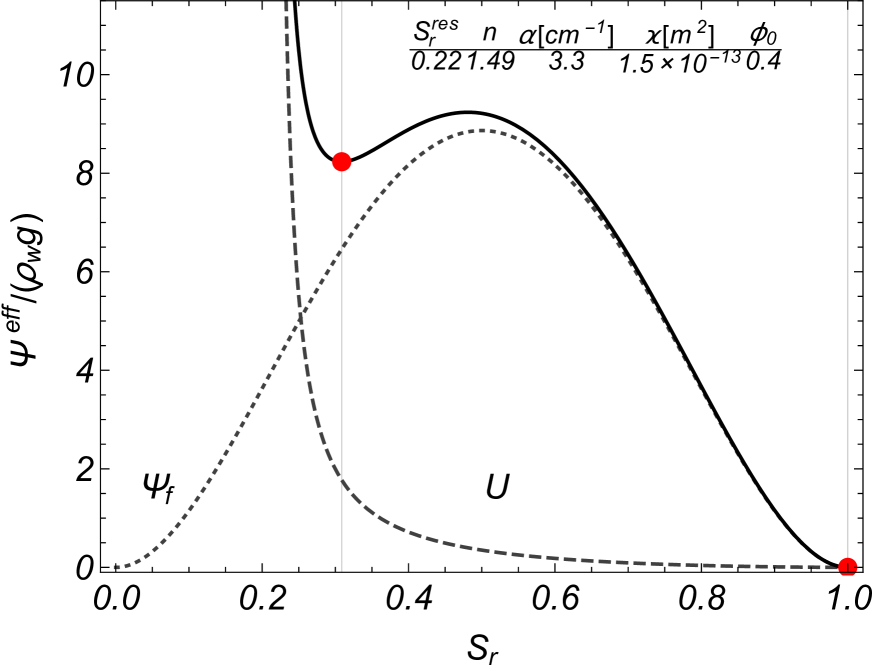
(g) Sandy clay Loam

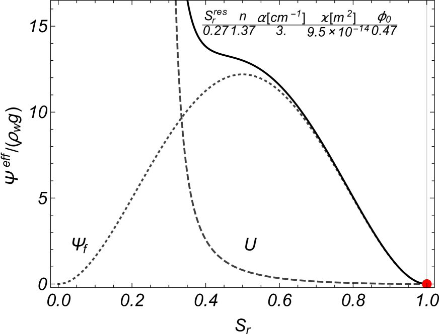
(h) Clay loam

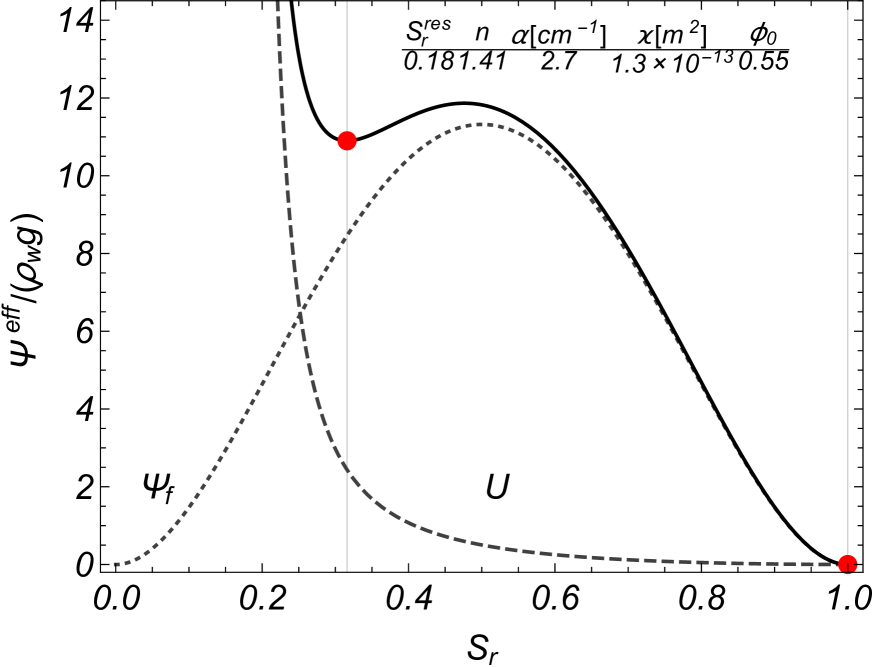
(i) Silty clay loam

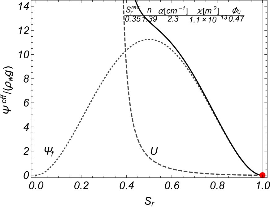
(j) Silty clay

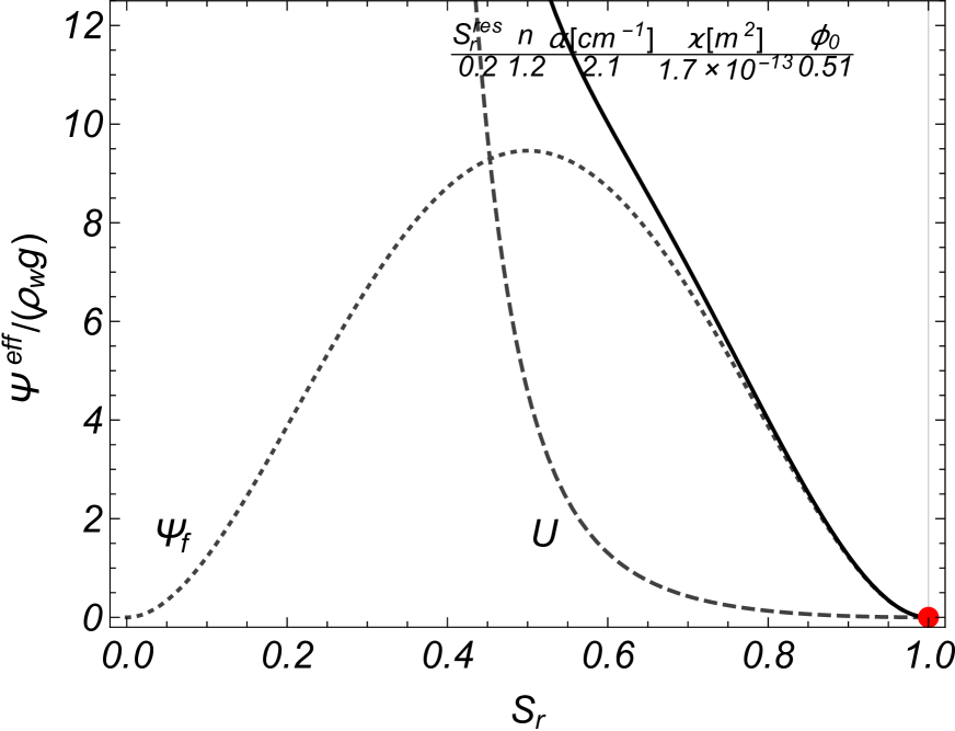
(k) Clay

Figure 3: Energy of the pure fluid $\Psi_{f}$ (dotted gray line), capillary energy $U$ (dashed gray line) and effective pore-fluid energy (solid black line). The values of the parameters which characterize the capillary energy are those of the retention curve (47) and are listed in each panel, together with the intrinsic permeability $\varkappa$ and the referential porosity $\phi_{0}$, relative to the portion of sand, clay and silt which constitute the soil. The red spots indicate the minima of the pore-fluid energy $\Psi_{f}+U$ which maintains a double-well shape in panels (a), (b), (c), (g) and (i).

It is worth to underline that the negative effective chemical potential exhibits, for all the considered textures, a non-monotonic behavior and in panels $(a)$, $(b)$, $(c)$, $(g)$ and $(i)$ two additional zeros (the spots) with respect to that at $S_{r}=1$, which can always be found. This feature corresponds to the fact that the effective pore-fluid energy $\Psi_{f}+U$ maintains the double-well shape typical of $\Psi_{f}$, see panels $(a)$, $(b)$, $(c)$, $(g)$, $(i)$ of Figure 3. The two minima of $\Psi_{f}+U$ are however no more isopotential and the one associated to the smallest value of $S_{r}$ has been shifted inwards the interval $(0,1)$. As already noticed the correction provided by $U$ to $\Psi_{f}$ allows therefore to account for the wetting properties of the grains, which do not permit the whole fluid to escape from the pore space even when a vanishing chemical potential is assumed. In all the other cases the non-monotonic behavior of $\mu^{\textrm{eff}}$ does not correspond to additional stationary states of the pore-fluid as the energy $\Psi_{f}+U$ exhibits only one minimum.

This non-monotonic behavior of the effective chemical potential resembles that one postulated by [47] in order to explain the formation of gravity fingers in soils. However it is worth to underline, following [34], that the appropriate form of the potential $-\partial U/\partial S_{r}$ is captured solving an inverse problem which stems from experimental evidence. As a consequence, the effective generalized chemical potential $\text{\textmu}^{\textrm{eff}}$ can indeed be hydrostatic at equilibrium, and therefore consistent with gravitational loading, even if the effective chemical potential $\mu^{\textrm{eff}}$ is not.

6 Micro-scale interpretation of the enhanced constitutive prescription of capillary pressure

In order to compare the enhanced model of capillary pressure (37) with the classical one, see e.g. [29, 30], the dependence of the free energy $\Psi_{s}$ on the saturation degree $S_{r}$ is concentrated, as already done in § 4.2 and § 5, in the capillary energy $U$ multiplied by the Lagrangian porosity, say $\phi U(S_{r})$. Equation (37)₁ therefore explicitly improves the basic constitutive prescription of the macro-scale capillary pressure by a correction depending on the gradient of the Jacobian determinant $J$ and the gradient of the water content $nS_{r}$, once the quadratic form (17) for the non-local contribution to the energy of the fluid has been assumed:

$$\mathcal{P}_{c}=-\dfrac{\partial U}{\partial S_{r}}-\dfrac{\mathrm{C}_{\kappa}}{J^{2}}\left(F^{-1}\right)_{m\alpha}\left(F^{-1}\right)_{k\alpha}\left[(\phi S_{r})_{,m}-(\phi S_{r})\frac{J_{,m}}{J}\right]\,J_{,k}.$$ (48)

When the hyper-stress acting on the non-uniform fluid vanishes, this correction vanishes as well; in other words the larger the gradient of the liquid content is, the wider the discrepancy between the standard and the enhanced constitutive prescriptions of $\mathcal{P}_{c}$ will be. The enhanced constitutive prescription (48) is expected therefore to yield significant modifications of the capillary pressure, in the narrow subdomains of the current shape of the porous medium where significant gradients of the liquid content can be detected. This justifies the claim of an interpretation of this contribution in terms of the so-called specific interfacial area.

According to the experimental data, reported among others by [40, 39] and [28], and the pore-network numerical simulation of quasi-static drainage and imbibition of a porous medium, see e.g. [64], local variations of the macroscopic capillary pressure are typically accompanied not only by changes in the saturation degree but also by changes in the interfacial area $a_{nw}$, which accounts for the local cumulative measure of the interfaces between the non-wetting and the wetting phase, per unit volume of the RVE. Apparently changes in the interfacial area may or may not result into an incoming or an outcoming flow through the RVE, however, in the spirit of providing an interpretation of the considered macro-scale model of the capillary force, in terms of possible effects of the interfacial area, only the variations of $a_{nw}$, which are associated to a flow through the boundary of the RVE are considered, whilst no account is taken of those variations which yield a pure remodeling of the internal structure of the RVE. In other words a relation between the interfacial area and the gradient of the saturation degree is expected to be identified, only if the liquid particles are displaced towards the boundary of the RVE.

To verify the validity of this hypothesis a heuristic micro-scale analysis is developed deforming a prototype initial configuration $\mathcal{B}^{0}$ of a RVE by a quasi-static loading path driven by the Lagrangian gradient of the macro-scale Jacobian determinant $J$; the liquid is squeezed out of the porous chamber along the same direction of the gradient of $J$. The saturation degree $S_{r}$ is assumed to be not affected by the considered micro-scale deformation, which means that the ratio between the volume of liquid and the volume of the pores within the RVE does not vary during the considered deformation process. This assumption allows to capture the correction to the constitutive prescription of $\mathcal{P}_{c}$ provided by the gradient term of the fluid energy only. In Figure 4 possible initial configurations of the RVE, parametrized by the degree of saturation are depicted; the dashed lines delimitate the boundary of the reference shapes.

(a) $S_{r}=0.441132$

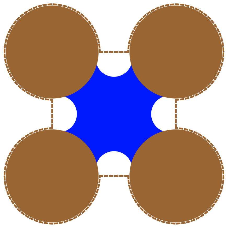
(b) $S_{r}=0.667298$

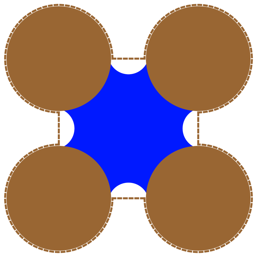
(c) $S_{r}=0.834704$

Figure 4: Referential RVEs parametrized by the saturation degree; the dashed line indicates the boundary of the RVE. The distance between the beads, made dimensionless with respect to the characteristic size of the RVE, is $L=0.25$, whilst their radius is $R=(1-L)/2$. $(X_{1},X_{2})$ indicates coordinate system in the reference configuration.

Each RVE corresponds to the deformed current configuration $\mathcal{B}$ of an initial domain $\mathcal{B}^{0}$ constituted by four identical beads among which a suitable amount of liquid water (the wetting phase) is trapped by capillary forces. The amount of liquid (in volume) is prescribed by the value of the degree of saturation; on the other hand its spatial distribution is a function of the local wetting properties of the beads. Here, for the sake of simplicity, the equilibrium value of Young’s contact angle is kept constant during deformation and circular interfaces between the non-wetting and the wetting fluid are assumed at each loading step. Tuning the parameterizing value of $S_{r}$ is expected to provide a-posteriori the relation between the specific interfacial area and the saturation degree, and consequently to compare the results of the model with the benchmark experimental data, relative to drainage-imbibition cycles.

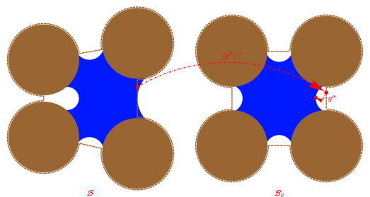
Figure 5: On the left a possible RVE, say $\mathcal{B}$, on the right its referential counter image, say $\mathcal{B}^{0}$. The map $g^{\textrm{m}}$ associates to each point of the reference configuration, which is mapped by $\chi^{\textrm{m}}$ into the current position of a liquid particle, the corresponding position in the initial configuration of the liquid.

Let $\chi^{\textrm{m}}$ and $g^{\textrm{m}}=(\chi_{liq}^{\textrm{m}})^{-1}\circ\chi^{\textrm{m}}$ be the micro-scale placement of the solid and the pull-back, in the solid reference configuration, of the inverse of the micro-scale placement of the liquid $\chi_{liq}^{\textrm{m}}$, respectively; they are diffeomorphisms over the above mentioned reference configuration, similarly to the corresponding macro-scale maps introduced in § 1. In particular $\chi^{\textrm{m}}$, which is naturally defined over the reference configuration of the solid $\mathcal{D}_{s}^{0}$, is extended over the pore space network. On the other hand the domain of $g^{\textrm{m}}$ is the subset $\mathcal{D}^{0}_{liq}$, of the reference configuration, mapped by $\chi^{\textrm{m}}$ into the inter-granular space occupied by the liquid in the current configuration. Notice that $\mathcal{D}^{0}_{liq}$ does not coincide with the initial configuration of the liquid, but it is the pull-back of the current shape of the liquid into the reference (initial) configuration of the solid grains, see Figure 5.

Let $x$, which indicates the macro-scale placement in the current configuration of the porous medium, be the centroid of the considered RVE and let $z$ be the micro-scale current position of a solid or a liquid particle within the RVE; the corresponding placements in the reference configuration of the solid are $X$ and $Z$, respectively. In Figures 6-8 different RVEs are depicted, which are obtained by deforming the prototype initial configurations, reported in Figure 4, by the above mentioned loading path driven by the gradient of $J$. In particular the deformation is achieved by the relative motion of the beads. For the sake of simplicity a quadratic displacement field, defined over the referential domain enclosed by the centers of the beads, is assumed for describing this deformation mechanism, even if the beads suffer just mutual translations. Considering a local coordinate system, with the origin in the centroid of the reference shape of the RVE, the micro-scale displacement is therefore assigned as

$$u_{i}^{\textrm{m}}(Z)=\chi_{i}^{\textrm{m}}(Z)-Z_{i}=a\,Z_{i}+\frac{1}{2}\mathbb{A}_{ijk}\,Z_{j}Z_{k}.$$ (49)

A representation formula for the displacement of the liquid, with respect to its initial configuration, is not stated, but suitable assumptions on its admissible current configuration are required. As already noticed the liquid is squeezed out of the pore due to the mutual displacement of the beads. In Appendix C the parametrization of the domain occupied by the liquid at each loading step is illustrated in details. The micro-scale parametrization (49) of the displacement of the grains and the hypotheses on the displacement of the liquid provide a micro-scale interpretation of the macro-scale gradients of the Jacobian determinant $J$ and the volume liquid content $\phi S_{r}$, by recalling the notion of averaging operators relative to the solid and the liquid constituent, see for more details [72], and [48]. As a matter of fact the macroscopic gradients of $J$ and $\phi S_{r}$, introduced in equation (48), can be explicitly calculated, starting from the micro-scale data, as the integrals over the counter image under $\chi^{\textrm{m}}$ of those parts of the boundary of the RVE occupied by solid or liquid particles, if any:

$$J_{,k}=JF_{\alpha i,k}\,F^{-1}_{i\alpha};\quad F_{\alpha i}(X):=\left(\displaystyle\int_{\mathcal{D}_{s}^{0}\cap\mathcal{B}^{0}}{\hskip-31.72498pt-}{\hskip 22.0507pt}F^{\textrm{m}}_{\alpha i}(Z)\right),\quad F_{\alpha i,k}(X):=\left(\displaystyle\int_{\partial(\mathcal{D}_{s}^{0}\cap\mathcal{B}^{0})\backslash\mathcal{I}^{0}_{s}}{\hskip-55.3408pt-}{\hskip 48.36958pt}F^{\textrm{m}}_{\alpha i}(Z)\,\nu_{k}^{0}\right),$$ (50)

$$(\phi S_{r})_{,k}=(\phi S_{r})\,G_{li,k}\,G^{-1}_{il};\quad G_{li}(X):=\left(\displaystyle\int_{\mathcal{D}_{liq}^{0}\cap\mathcal{B}^{0}}{\hskip-36.27708pt-}{\hskip 24.89615pt}G^{\textrm{m}}_{li}(Z)\right),\quad G_{li,k}(X):=\left(\displaystyle\int_{\partial(\mathcal{D}_{liq}^{0}\cap\mathcal{B}^{0})\backslash\mathcal{I}^{0}_{f}}{\hskip-60.4621pt-}{\hskip 51.21504pt}G^{\textrm{m}}_{li}(Z)\,\nu_{k}^{0}\right).$$ (51)

In equations (50)-(51) $\int\hskip-9.38945pt-$ indicates the average integral over the reference configuration of the RVE, i.e. the integral divided by the volume of $\mathcal{B}^{0}$, moreover $F^{\textrm{m}}$ and $G^{\textrm{m}}$ are the gradients of the maps $\chi^{\textrm{m}}$ and $g^{\textrm{m}}$, respectively. At the micro-scale, $\mathcal{D}_{s}^{0}\cap\mathcal{B}^{0}$ ($\mathcal{D}_{liq}^{0}\cap\mathcal{B}^{0}$) is the intersection between the reference shape of the solid grains, say $\mathcal{D}^{0}_{s}$, (the pull-back of the current shape of the liquid in the reference configuration of the solid, say $\mathcal{D}^{0}_{liq}$) with the reference configuration of the RVE, which corresponds to that part of the reference shape occupied by the beads (liquid). On the other hand $\partial(\mathcal{D}_{s}^{0}\cap\mathcal{B}^{0})\setminus\mathcal{I}^{0}_{s}$ ($\partial(\mathcal{D}_{liq}^{0}\cap\mathcal{B}^{0})\setminus\mathcal{I}^{0}_{f}$) is the counter image of the boundary of the RVE occupied by the solid (liquid) particles, in the reference configuration. A detailed deduction of equations (51) is developed in Appendix D, together with a remark on a possible way to estimate the macro-scale field $G_{li,k}$ in terms of the micro-scale gradient of $g^{\mathrm{m}}$.

The scalar quantity $a$ and the third order tensor $\mathbb{A}_{ijk}$, in equation (49), coincide with the spherical part of $F_{\alpha i}$ and the macro-scale second gradient of deformation $F_{\alpha i,k}$, respectively. This last is supposed to be characterized by a unique non-vanishing contribution $\mathbb{A}_{221}=F_{22,1}$, which implies the gradient of $J$ to be along the abscissa $X_{1}$. The spherical part of the deformation gradient on the other hand is determined so as to keep constant the degree of saturation and to allow the liquid phase to form a meniscus concave towards the gaseous phase outside the RVE and tangent to its boundary. The liquid is displaced along the same direction of the gradient of the Jacobian determinant, see Figures 6(b)-6(d), 7(b)-7(d) and 8(b)-8(d).

As already noticed the contact angle between the solid and the liquid is kept constant, during the deformation process, and the interfaces between the wetting and the non-wetting phase maintain a circumferential shape. The smaller the saturation $S_{r}$ is the less realistic this assumption will be, see Figure 4(a). Being required to simplify the calculations, it therefore remains valid only for values of $S_{r}$ which do not allow thin capillary bridges to form.

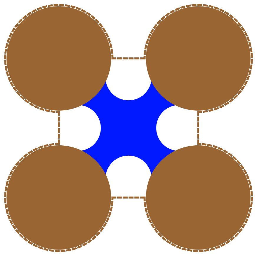
(a) $J_{,1}=0$

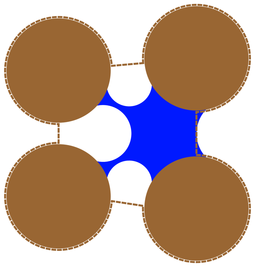
(b) $J_{,1}=0.173618$

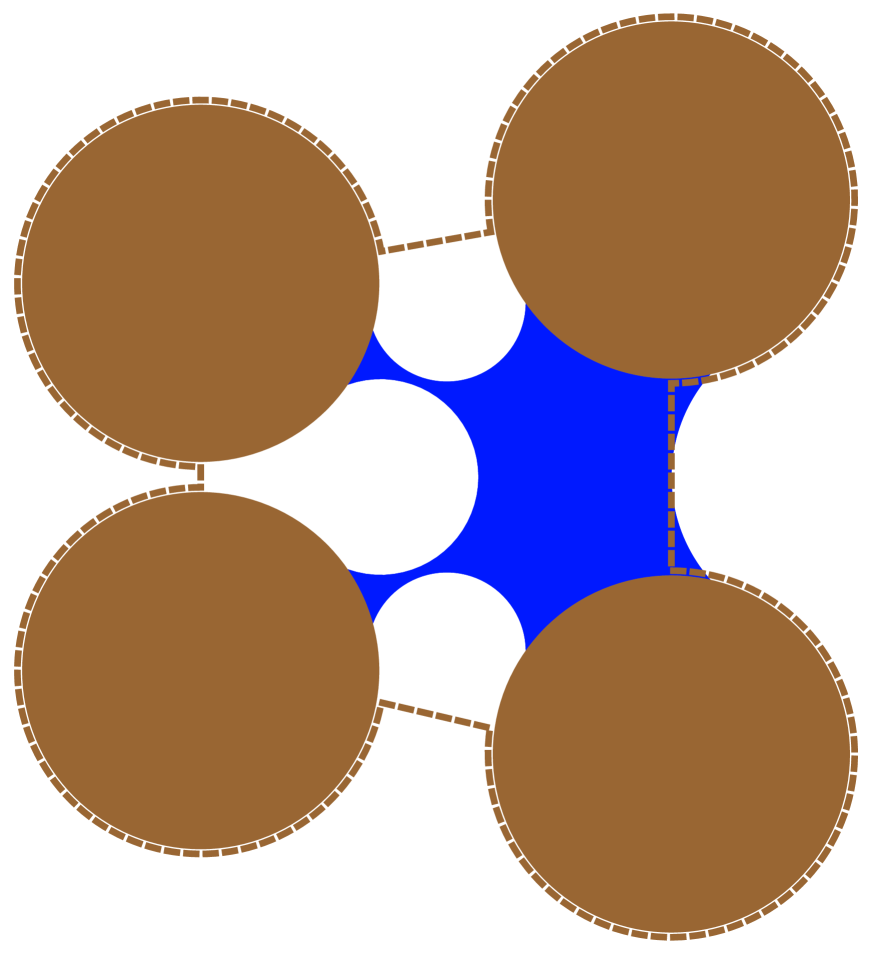
(c) $J_{,1}=0.347235$

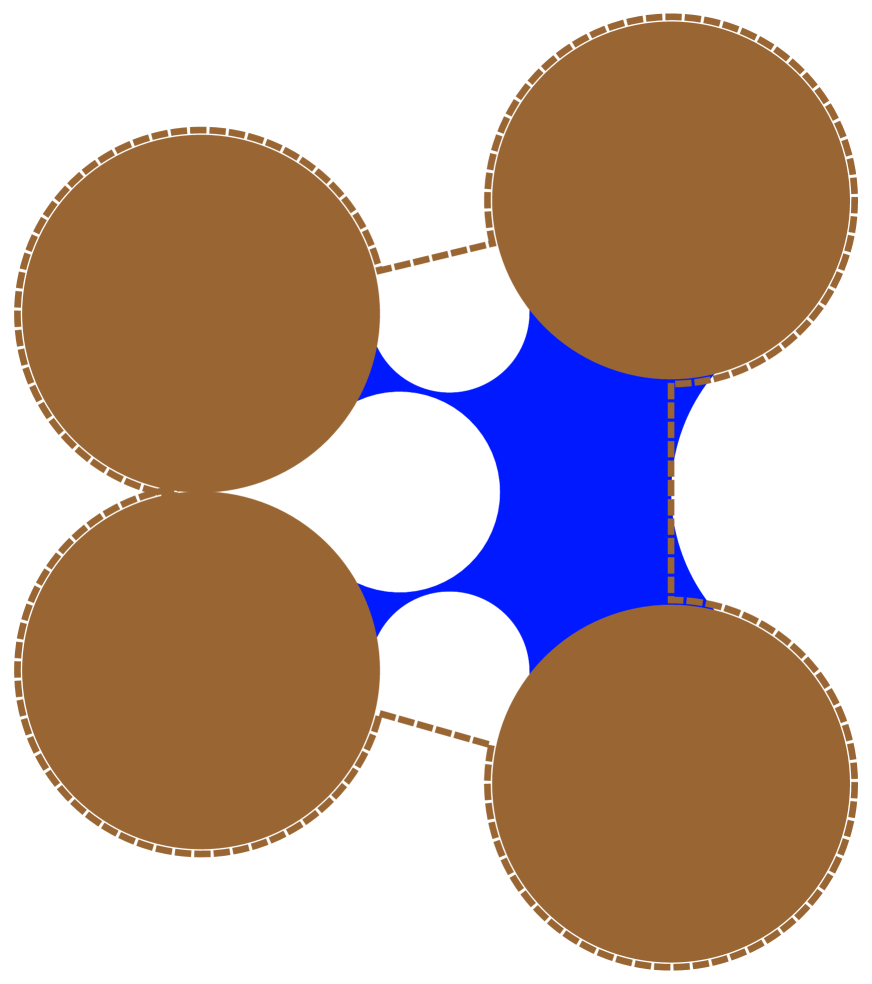
(d) $J_{,1}=0.471248$

Figure 6: Admissible distributions of the liquid phase within different RVEs, which are obtained as the current configurations of the reference shape reported in panel (a). The micro-scale displacement of the solid beads is parametrized by the value of $J_{,1}$ via its dependence on the macro-scale second gradient of deformation. During the deformation the saturation ratio is kept constant: $S_{r}=0.441132$ (see Figure 4(a)).

(a) $J_{,1}=0$

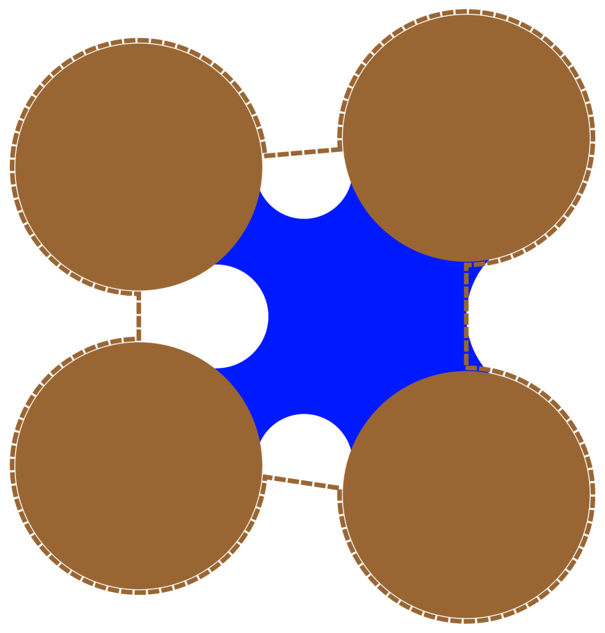
(b) $J_{,1}=0.173618$

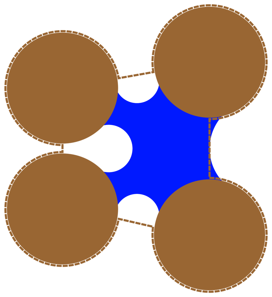
(c) $J_{,1}=0.347235$

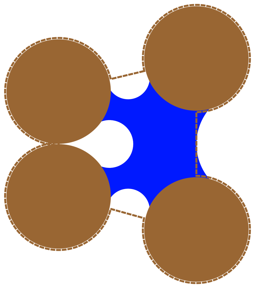
(d) $J_{,1}=0.471248$

Figure 7: Admissible distributions of the liquid phase within different RVEs, which are obtained as the current configurations of the reference shape reported in panels (a) and (e). The micro-scale displacement of the solid beads is parametrized by the value of $J_{,1}$ via its dependence on the macro-scale second gradient of deformation. During the deformation the saturation ratio is kept constant: $S_{r}=0.667298$ (see Figure 4(b)).

(a) $J_{,1}=0$

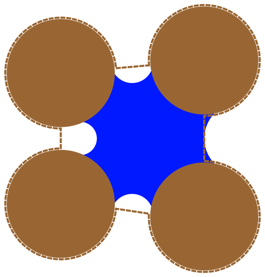
(b) $J_{,1}=0.173618$

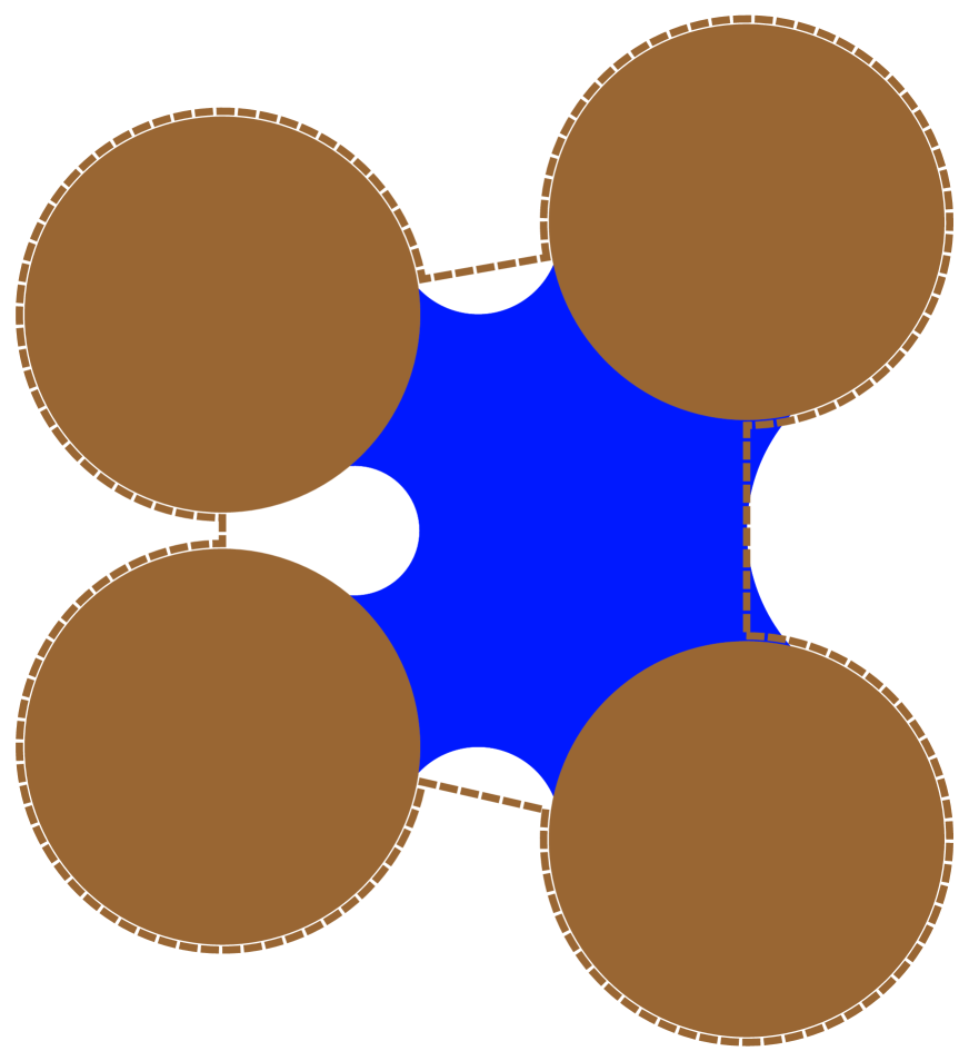
(c) $J_{,1}=0.347235$

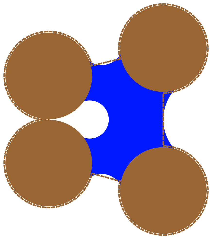
(d) $J_{,1}=0.471248$

Figure 8: Admissible distributions of the liquid phase within different RVEs, which are obtained as the current configurations of the reference shape reported in panels (a) and (e). The micro-scale displacement of the solid beads is parametrized by the value of $J_{,1}$ via its dependence on the macro-scale second gradient of deformation. During the deformation the saturation ratio is kept constant: $S_{r}=0.882695$ (see Figure 4(c)).

Equations (50) and (51) motivate the conjecture assumed at the beginning of this section on the effects of the average interfacial area $a_{nw}$ on the macroscopic capillary pressure. As a matter of fact they imply that the corrective terms in equation (48) are not zero only if the integrals over specific parts of the boundary of the reference configuration of the RVE do not vanish. In other words the fluid trapped among the beads must attain the boundary in order for the gradient of the liquid content to not fade away. Thus in order to prove a functional correlation between gradient of $\phi S_{r}$ and interfacial area, all the micro-scale deformations which do not drive the liquid to the boundary of the RVE should not be taken into account.

Considering the geometrical data reported in the caption of Figure 4 and the above mentioned assumptions on the maps $\chi^{\textrm{m}}$ and $g^{\textrm{m}}$, the corrective terms of capillary pressure introduced in equation (48) can be explicitly calculated by means of equations (50)-(51). At the same time the average interfacial area consistent with the envisaged liquid distribution, can be estimated for each value of $J_{,1}$. A contour plot of the constitutive law (48) parametrized by the obtained value of $a_{nw}$ could therefore be drawn, see Figure 9.

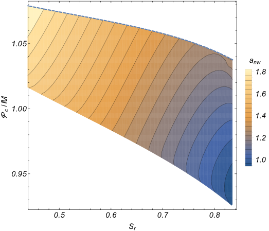
Figure 9: The capillary pressure $\mathcal{P}_{c}$ is represented as a function of the saturation ratio $S_{r}$, within the interval delimited by the maximum and the minimum value of $S_{r}$ reported in Figure 4 and parametrized by the interfacial area $a_{nw}$. The dashed line denotes to the locus of maximum values of $\mathcal{P}_{c}$ due to the gradient corrective terms.

Indeed it qualitatively resembles the one traced in [64, Figure 11], for the values of the saturation degree which have been considered in the present analysis. However it is worth to notice that the considered deformation and flow regimes are totally different with respect to those simulated by [64], as they are driven by the gradient of the Jacobian $J$, at different values of $S_{r}$, whilst those ones of [64] are deduced simulating many scanning loops of drainage and imbibition. This is indeed an interesting point which corroborates the idea, introduced in the seminal paper of [59], of resolving the hysteresis of the capillary pressure, between drainage and imbibition, introducing a suitable micro-structural parameter, say $a_{nw}$, which tunes the value of $\mathcal{P}_{c}$ for each value of $S_{r}$.

For the considered values of the saturation degree, the distribution of the interfacial area is plotted against the capillary pressure in Figure 10; again the result is consistent with the experimental evidence reported in [28], [39] and [40]. Comparing the envisaged relation with that one deduced by [40, Figure 10b] and [39, Figure 7b] one can notice that consistency with the experimental data is achieved when the capillary pressure is not too large, in particular not larger than a suitable inversion point, see [40, Figure 10],

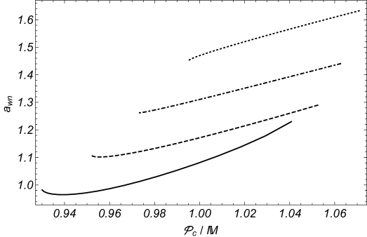
Figure 10: Average interfacial area, calculated from the liquid spatial distribution within the RVE, vs capillary pressure, calculated on the basis of equation (48), taking in due account the definitions (50)-(51) of macro-scale gradients in terms of the micro-scale maps $\chi^{\textrm{m}}$ and $g^{\textrm{m}}$. The solid line corrsponds to $S_{r}=0.8197$, the dashed line to $S_{r}=0.7394$, the dot-dashed line to $S_{r}=0.6479$ and the dotted line to $S_{r}=0.5411$.

in Figure 11 the projection of the $\mathcal{P}_{c}$-$S_{r}$-$a_{nw}$ relation on the $S_{r}$-$a_{nw}$ plane is finally depicted for the considered distribution of the liquid phase within the RVE during the deformation process. Again a comparison with the experimental result of [40] and [39] confirms the validity of the obtained results for the considered range of values of $S_{r}$ and $\mathcal{P}_{c}$.

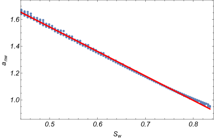
Figure 11: Linear regression of data relative to the calculated admissible values of $S_{r}$ and $a_{nw}$, deduced from the micro-scale analysis.

The considered micro-scale analysis showed an a-posteriori relation between the average interfacial area $a_{nw}$ and the gradient of the liquid content, in the presence of a non-trivial flow through the boundary of the RVE. As the average interfacial area is typically parametrized by the pore size distribution, the higher order constitutive parameter $\mathrm{C}_{k}$ should also depend on it so that the more the collection of pores, forming the RVE, is non-uniform, the more the micro-scale deformations of the skeleton will affect the retention properties of the porous material. The pore size polydispersity is therefore expected to highly affect the corrective term to $\mathcal{P}_{c}$ reported in equation (48) (the higher the polydispersity, the larger the gradient corrective term).

It is worth to underline that the considered micro-scale analysis stems from the assumption of non-negligible strain gradients, which in fact parametrize the deformation process, even if only small strain of the solid skeleton are considered. If, on the other hand, this assumption were not valid, equation (37)₁ would abruptly simplify into the standard constitutive prescription of capillary pressure.

7 Governing equations

Restrictions due to thermodynamics have provided a consistent representation of the overall free energy of the porous continuum $\Psi$, as the sum of the free energy of the skeleton and the interfaces $\Psi_{s}$ and that of the bulk fluid $\Psi_{f}$, weighted by Lagrangian porosity, in terms of strain, Lagrangian porosity, saturation degree, strain gradient and gradient of liquid content. This characterization has been deduced postulating the balance of momentum for the overall porous medium, and exploiting the Clausius-Duhem inequality; the constitutive prescription of the local fluid flux, say the generalized Darcy law, has also been obtained. However no explicit deduction of the boundary conditions relative to the partial differential equations associated to the overall equilibrium (7) and the generalized Richards equation (43) or (45) have been stated.

In this section the governing equations, and the corresponding boundary conditions, for an unsaturated porous medium, within the framework of the adopted regularized phase field model, are deduced by means of a variational approach. To do this the independent variations of $\chi_{\alpha}$, $g_{k}$ and $\phi$, $\forall X\in\mathcal{D}_{0}$, are taken into account. Let

$$\chi_{\alpha}^{\ast}\left(X,t\right)=\chi_{\alpha}\left(X,t\right)+\delta\chi_{\alpha}\left(X,t\right),\quad g_{j}^{\ast}\left(X,t\right)=g_{j}\left(X,t\right)+\delta g_{j}\left(X,t\right),\quad\phi^{\ast}\left(X,t\right)=\phi\left(X,t\right)+\delta\phi\left(X,t\right),$$ (52)

be the varied fields, and $\delta\chi_{\alpha}$, $\ \delta g_{k}$ and $\delta\phi$ the corresponding arbitrary variations. The physical meaning of the variation $\delta\chi_{\alpha}$ is well known in continuum mechanics and stands for the virtual displacement (deformation) of the solid skeleton. In the following this variation will also be indicated as $\delta u$, which corresponds to the varied displacement field $u^{\ast}$. The variation $\delta g_{k}$, instead, accounts for the virtual relative displacement of a fluid material particle with respect to a solid one. The variation $\delta\phi$ finally indicates the local change of Lagrangian porosity. All these variations are evaluated keeping fixed $X\in\mathcal{D}_{0}$, therefore $\delta$ commutes with the Lagrangian gradient operator and can enter the integral over $\mathcal{D}_{0}$.

Following the statements of classical mechanics, the principle of virtual working reads

$$\delta\mathcal{A=}-\delta\mathcal{L}^{\mathrm{ext}}-\delta\mathcal{L}^{\mathrm{diss}}$$ (53)

where $\delta\mathcal{A}$ represents the Lagrangian variation of the action functional defined, neglecting inertia effects, as

$$\mathcal{A}:=-\displaystyle\int_{\mathcal{D}_{0}}\left(\Psi_{s}+m_{f}\psi_{f}\right),$$ (54)

while $\delta\mathcal{L}^{\mathrm{diss}}$ and $\delta\mathcal{L}^{\mathrm{ext}}$ are the virtual working due to dissipative forces and the virtual working of external forces, respectively. The virtual working of dissipative forces is

$$\delta\mathcal{L}^{\mathrm{diss}}=\displaystyle\int_{\mathcal{D}_{0}}\left(\mathrm{det}G\right)(1/\rho_{L})A_{kl}M_{l}\left(G^{-1}\right)_{kj}\delta g_{j},$$ (55)

see [89], whilst the virtual working of external forces can be stated in a similar form as that in equation (4). The virtual velocities $v_{\alpha}^{s}$ and $v_{\alpha}^{f}$ are replaced by the virtual displacements $\delta\chi_{\alpha}$ and $\delta\chi_{\alpha}^{f}=\delta\chi_{\alpha}-F_{\alpha k}(G^{-1})_{kj}\delta g_{j}$, respectively:

$$\begin{array}[]{ll}\delta\mathcal{L}^{\mathrm{ext}}&=\displaystyle\int_{\partial\mathcal{D}_{0}}\left\{t_{\alpha}^{0}\delta\chi_{\alpha}+\tau_{\alpha}^{0}\delta\chi_{\alpha,k}\,n_{k}-\left[t_{k}^{0f}\left(G^{-1}\right)_{kj}\delta g_{j}+\tau^{0f}_{k}\left(G^{-1}\right)_{kj}\delta g_{j,l}\,n_{l}\right]\right\}\vskip 6.0pt plus 2.0pt minus 2.0pt\\ &+\displaystyle\int_{\mathcal{E}_{0}}\left[f_{\alpha}^{0}\delta\chi_{\alpha}-f_{k}^{0f}\left(G^{-1}\right)_{kj}\delta g_{j}\right]+\displaystyle\int_{\mathcal{D}_{0}}\left[b_{\alpha}^{0}\delta\chi_{\alpha}-b_{k}^{0f}\left(G^{-1}\right)_{kj}\delta g_{j}\right],\end{array}$$ (56)

where the referential bulk forces ($b^{0}_{\alpha}$ and $b^{0f}_{k}$), the surface tractions ($t^{0}_{\alpha}$ and $t^{0f}_{k}$), the surface double forces ($\tau^{0}_{\alpha}$ and $\tau^{0f}_{k}$) and the line tractions ($f^{0}_{\alpha}$ and $f^{0f}_{k}$) are defined in terms of the corresponding forces acting on the current shape of the porous continuum as follows, for the overall porous medium

$$\begin{array}[]{ll}t_{\alpha}^{0}=&\!\!\!J^{s}t_{\alpha}-\left[J^{s}\tau_{\alpha}Q_{Bl}\left(F^{-1}\right)_{l\beta}\left(F^{-1}\right)_{k\beta}n_{k}\right]_{,B},\quad b_{\alpha}^{0}=Jb_{\alpha},\vskip 6.0pt plus 2.0pt minus 2.0pt\\ \tau_{\alpha}^{0}=&\!\!\!J^{s}\tau_{\alpha}\left(F^{-1}\right)_{l\beta}n_{l}\left(F^{-1}\right)_{k\beta}n_{k},\vskip 6.0pt plus 2.0pt minus 2.0pt\\ f_{\alpha}^{0}=&\!\!\!J^{l}f_{\alpha}+\left[\!\!\left[J^{s}\tau_{\alpha}Q_{Bl}\left(F^{-1}\right)_{l\beta}\left(F^{-1}\right)_{k\beta}n_{k}\,\nu_{B}\right]\!\!\right];\end{array}$$ (57)

and for the fluid

$$\begin{array}[]{ll}t_{k}^{0f}=&\!\!\!J^{s}\left[F_{\alpha k}t_{\alpha}^{f}+\tau_{\alpha}^{f}\left(F_{\alpha r}\left(G^{-1}\right)_{rq}\right)_{,l}\left(F^{-1}\right)_{l\beta}\left(F^{-1}\right)_{p\beta}n_{p}G_{qk}\right]+\vskip 6.0pt plus 2.0pt minus 2.0pt\\ &-\left[J^{s}F_{\alpha r}\tau_{\alpha}^{f}\left(G^{-1}\right)_{rq}Q_{Bl}\left(F^{-1}\right)_{l\beta}\left(F^{-1}\right)_{p\beta}n_{p}\right]_{,B}G_{qk},\quad b_{k}^{0f}=JF_{\alpha k}b_{\alpha}^{f},\vskip 6.0pt plus 2.0pt minus 2.0pt\\ \tau_{k}^{0f}=&\!\!\!J^{s}F_{\alpha k}\tau_{\alpha}^{f}\left(F^{-1}\right)_{l\beta}n_{l}\left(F^{-1}\right)_{p\beta}n_{p},\vskip 6.0pt plus 2.0pt minus 2.0pt\\ f_{k}^{0f}=&\!\!\!J^{l}F_{\alpha k}f_{\alpha}^{f}+\left[\!\!\left[J^{s}F_{\alpha k}\tau_{k}^{f}Q_{lB}\left(F^{-1}\right)_{l\beta}\left(F^{-1}\right)_{p\beta}n_{p}\,\nu_{B}\right]\!\!\right].\end{array}$$ (58)

In equations (57) and (58) $J^{s}$ and $J^{l}$ indicate the determinant of the surface and line restrictions of $F$ over the boundary of $\mathcal{D}_{0}$ and its edges. According to equations (54) and (31) the variation of the free energy is

$$\begin{array}[]{ll}\delta\mathcal{A}=-\displaystyle\int_{\mathcal{D}_{0}}\!\!\!\!\!&\left(\dfrac{\partial\Psi_{s}}{\partial E_{ij}}\delta E_{ij}+\dfrac{\partial\Psi_{s}}{\partial E_{ij,k}}\delta E_{ij,k}+\dfrac{\partial\Psi_{s}}{\partial\phi}\delta\phi+\dfrac{\partial\Psi_{s}}{\partial S_{r}}\delta S_{r}\right.\vskip 6.0pt plus 2.0pt minus 2.0pt\\ &\left.+\dfrac{\partial\Psi_{s}}{\partial\left(\phi S_{r}\right)_{,l}}\delta\left(\phi S_{r}\right)_{,l}+\,\rho_{L}\psi_{f}\delta\left(\phi S_{r}\right)+\phi S_{r}\dfrac{\partial\psi_{f}}{\partial(1/\rho_{f})}\delta\left(\dfrac{1}{S_{r}}\right)\right),\end{array}$$ (59)

where the following identities hold true:

$$\begin{array}[]{ll}\delta E_{ij}&=\dfrac{1}{2}\left(\delta F_{\alpha i}F_{\alpha j}+F_{\alpha i}\delta F_{\alpha j}\right),\vskip 6.0pt plus 2.0pt minus 2.0pt\\ \delta E_{ij,k}&=\dfrac{1}{2}\left(\delta F_{\alpha i,k}F_{\alpha j}+\delta F_{\alpha j,k}F_{\alpha i}\right)+\dfrac{1}{2}\left(\delta F_{\alpha i}F_{\alpha j,k}+\delta F_{\alpha j}F_{\alpha i,k}\right),\vskip 6.0pt plus 2.0pt minus 2.0pt\\ \delta\left(\phi S_{r}\right)&=\mathrm{det}G\left(G^{-1}\right)_{kj}\delta g_{j,k},\quad\delta S_{r}=\dfrac{1}{\phi}\delta\left(\phi S_{r}\right)-\dfrac{S_{r}}{\phi}\delta\phi.\end{array}$$ (60)

The local governing equations are deduced by requiring the validity of equation (53) for every kinematically admissible variation $\delta\chi_{\alpha}$, $\delta g_{j}$ and $\delta\phi$. To this aim, the distinction between essential ($e$) and natural ($n$) boundary conditions needs to be generalized, following the scheme proposed in [43]. On every part $\left(\mathcal{L}_{x}^{y}\right)_{c}\subset\partial\mathcal{D}_{0}$, with $x=e,n$, $y=e,n$, and for each constituent $c=\{s,f\}$, one may impose four different kind of boundary conditions, see Table 1 and Table 2.

$\left(\mathcal{L}_{e}^{e}\right)_{s}$	$u_{\alpha}=\overline{u}_{\alpha},$	$u_{\alpha,k}n_{k}=\overline{w}_{\alpha}$	$u$-essential	$D_{n}u$-essential
$\left(\mathcal{L}_{e}^{n}\right)_{s}$	$u_{\alpha}=\overline{u}_{\alpha},$	$\tau_{\alpha}=\overline{\tau}_{\alpha}$	$u$-essential	$\tau$-natural
$\left(\mathcal{L}_{n}^{e}\right)_{s}$	$t_{\alpha}=\overline{t}_{\alpha},$	$u_{\alpha,k}n_{k}=\overline{w}_{\alpha}$	$t$-natural	$D_{n}u$-essential
$\left(\mathcal{L}_{n}^{n}\right)_{s}$	$t_{\alpha}=\overline{t}_{\alpha},$	$\tau_{\alpha}=\overline{\tau}_{\alpha}$	$t$-natural	$\tau$-natural

Table 1: Generalized essential and natural boundary conditions relative to the porous skeleton.

$\left(\mathcal{L}_{e}^{e}\right)_{f}$	$g_{j}=\overline{g}_{j},$	$g_{j,k}n_{k}=\overline{\omega}_{j}$	$g$-essential	$D_{n}g$-essential
$\left(\mathcal{L}_{e}^{n}\right)_{f}$	$g_{j}=\overline{g}_{j},$	$\tau_{\alpha}^{f}=\overline{\tau}^{f}_{\alpha}$	$g$-essential	$\tau$-natural
$\left(\mathcal{L}_{n}^{e}\right)_{f}$	$t^{f}_{\alpha}=\overline{t}^{f}_{\alpha},$	$g_{j,k}n_{k}=\overline{\omega}_{j}$	$t$-natural	$D_{n}g$-essential
$\left(\mathcal{L}_{n}^{n}\right)_{f}$	$t^{f}_{\alpha}=\overline{t}^{f}_{\alpha},$	$\tau_{\alpha}^{f}=\overline{\tau}^{f}_{\alpha}$	$t$-natural	$\tau$-natural

Table 2: Generalized essential and natural boundary conditions relative to the non-uniform fluid.

Here the displacement $u$ rather than the placement $\chi$ of the solid particles is used and $(D_{n}u)_{\alpha}:=u_{\alpha,k}\,n_{k}$ and $(D_{n}g)_{j}:=g_{j,k}\,n_{k}$ indicate the normal derivatives of $u$ and $g$ along the outward normal to $\partial\mathcal{D}_{0}$. Subscripts distinguish $(u,g)$-essential from $t$-natural boundary conditions, whilst superscripts distinguish $D_{n}(u,g)$-essential from $\tau$-natural boundary conditions; moreover on every part of the $h$-th edge $\mathcal{E}_{h}$ the standard distinction between essential and natural conditions holds true. The varied maps $u^{*}$ and $g^{*}$ are said to be kinematically admissible if they satisfy the same essential boundary conditions as $u$ and $g$; as a consequence the variations $\delta u$ and $\delta g$ together with their normal derivative will vanish on $\left(\partial\mathcal{D}_{0}^{c}\right)^{\star}_{e}:=\left(\mathcal{L}^{e}_{e}\right)_{c}\cup\left(\mathcal{L}^{n}_{e}\right)_{c}$ and $\left(\partial\mathcal{D}_{0}^{c}\right)^{e}_{\star}:=\left(\mathcal{L}^{e}_{e}\right)_{c}\cup\left(\mathcal{L}^{e}_{n}\right)_{c}$, $c=\{s,f\}$, respectively. Replacing equations (60) into (59), and using standard localization arguments provides the following bulk equations in $\mathcal{D}_{0}$

$$\begin{array}[]{l}\left[F_{{\alpha}i}\,\left(S_{ij}-P_{ijk,k}\right)\right]_{,j}+b^{0}_{\alpha}=0,\vskip 6.0pt plus 2.0pt minus 2.0pt\\ \dfrac{\partial\Psi_{s}}{\partial\phi}-S_{r}\dfrac{\partial U}{\partial S_{r}}-\mathcal{P}=0,\vskip 6.0pt plus 2.0pt minus 2.0pt\\ \left[\dfrac{\partial(\Psi_{f}+U)}{\partial S_{r}}-\left(\dfrac{\partial\Psi_{s}}{\partial(\phi S_{r})_{,l}}\right)_{,l}\right]_{,k}=-\dfrac{1}{\rho_{L}}A_{kl}M_{l}+\dfrac{b_{k}^{0f}}{\phi S_{r}},\end{array}$$ (61)

where the notion of specific free energy of the fluid $\Psi_{f}$ (per unit volume) has been used together with that of capillary energy $U$. Equation (61)₁ states the equilibrium of the porous skeleton, equation (61)₂ the constitutive prescription of the thermodynamic pressure, which is the same as equation (35)₁, and equation (61)₃ the generalized Darcy law (41). At the same time the corresponding boundary conditions are provided, in particular traction boundary conditions are prescribed on $\left(\partial\mathcal{D}^{c}_{0}\right)^{\star}_{n}$, $c=\{s,f\}$

$$\begin{array}[]{l}F_{{\alpha}i}\,\left(S_{ij}-P_{ijk,k}\right)n_{j}-\left(Q_{Bj}F_{\alpha i}P_{ijk}n_{k}\right)_{,B}=t^{0}_{\alpha},\vskip 6.0pt plus 2.0pt minus 2.0pt\\ -\left[\dfrac{\partial(\Psi_{f}+U)}{\partial S_{r}}-\left(\dfrac{\partial\Psi_{s}}{\partial(\phi S_{r})_{,l}}\right)_{,l}\right]n_{k}+\left[\phi S_{r}\,Q_{Bj}\left(G^{-1}\right)_{j\ell}\left(\dfrac{\partial\Psi_{s}}{\partial(\phi S_{r})_{,l}}n_{l}\right)\right]_{,B}\dfrac{G_{\ell k}}{\phi S_{r}}=\dfrac{t^{0f}_{k}}{\phi S_{r}}\end{array}$$ (62)

double force boundary conditions are prescribed on $\left(\partial\mathcal{D}^{c}_{0}\right)^{n}_{\star}$, $c=\{s,f\}$

$$F_{\alpha i}P_{ijk}n_{k}n_{j}=J_{S}\tau_{\alpha},\quad-\phi S_{r}\left(\dfrac{\partial\Psi_{s}}{\partial(\phi S_{r})_{,l}}n_{l}\right)n_{k}=\tau^{0f}_{k},$$ (63)

and edge forces are prescribed on the $h$-th edge $\left(\mathcal{E}^{c}_{0h}\right)^{n}$ of $\mathcal{D}_{0}$,

$$\left[\!\left[Q_{Bj}F_{\alpha i}P_{ijk}n_{k}\nu_{B}\right]\!\right]=J_{L}f_{\alpha},\quad-\left[\!\!\left[\phi S_{r}Q_{Bk}\left(\dfrac{\partial\Psi_{s}}{\partial(\phi S_{r})_{,l}}n_{l}\right)\nu_{B}\right]\!\!\right]=f^{0f}_{k}.$$ (64)

As already mentioned these natural boundary conditions must be used together with the essential boundary conditions

$$\left\{\!\!\!\begin{array}[]{ll}u_{\alpha}=\overline{u}_{\alpha}&\textrm{on}\,\,\left(\partial\mathcal{D}^{s}_{0}\right)^{\star}_{e},\vskip 6.0pt plus 2.0pt minus 2.0pt\\ g_{\ell}\,\,=\overline{g}_{\ell}&\textrm{on}\,\,(\partial\mathcal{D}^{f}_{0})^{\star}_{e},\end{array}\right.\,\left\{\!\!\!\begin{array}[]{ll}u_{\alpha,k}\,n_{k}=\overline{w}_{\alpha},&\textrm{on}\,\,\left(\partial\mathcal{D}^{s}_{0}\right)^{e}_{\star},\vskip 6.0pt plus 2.0pt minus 2.0pt\\ g_{\ell,k}\,n_{k}\,\,=\overline{g}_{\ell},&\textrm{on}\,\,(\partial\mathcal{D}^{f}_{0})^{e}_{\star},\end{array}\right.\,\left\{\begin{array}[]{ll}\!\!\!u_{\alpha}=\overline{u}_{\alpha},&\textrm{on}\,\,(\mathcal{E}^{s}_{0h})^{e},\vskip 6.0pt plus 2.0pt minus 2.0pt\\ g_{\ell}=\overline{g}_{\ell},&\textrm{on}\,\,(\mathcal{E}^{f}_{0h})^{e}.\end{array}\right.$$ (65)

We underline that by definition $Q_{Bj}:=\partial\hat{X}_{B}/\partial X_{j}$, $\hat{X}_{B}$ is a system of coordinates which locally parametrizes $\partial\mathcal{D}_{0}$, moreover $\nu_{B}$ indicates the component of the Darboux tangent-normal vector to each edge of $\partial\mathcal{D}_{0}$.

8 Conclusions

In this paper gradient theory of poromechanics endowed with phase field modeling have been used to describe partial saturation. The spatial distribution of saturation and strain is spatially regularized, in the presence of phase coexistence, within the non-uniform fluid, and in the neighbors of possible heterogeneities in the porous skeleton. To do this the free energy of the overall porous medium has been regarded as a function not only of strain and saturation but also on their (Lagrangian) gradients.

As usual in gradient theories, the governing partial differential equations relative, in this case, to the solid skeleton and the non-uniform fluid are deduced using integration by parts twice, which implies the equations to be, in the general case, of the fourth order. In particular an enhanced version of classical Richards’ equation has been deduced from generalized Darcy’s law, which in the considered regime of partial saturation does not depend on the capillary pressure, but on the so-called generalized effective chemical potential.

Moreover a novel constitutive characterization of the capillary pressure is established and a micro-scale interpretation is provided, which is consistent with that originally formulated by [58, 59]. A comparison with experimental results also confirms that the contribution to capillary pressure due to saturation gradient allows for recovering similar effects as those captured by the average interfacial area.

In particular the model proposed in this paper aims at bridging the regularizing effects provided by the gradient of strain and the gradient of saturation in order to capture on one hand the response of the porous skeleton, due to micro-scale multi-phase flow, and on the other hand the heterogeneous and possibly anisotropic flow of the saturating fluids due to localized strains, induced by micro-structural remodeling processes. Further developments will be carried out in order to account for damaging and plastic strain.

Acknoledgements

The research has been partially supported by INdAM (Italian National Institute for Advanced Mathematics), within the framework of the “Young Researchers GNFM (National Group of Mathematical Physics)”  program. The author gratefully acknowledges this institution.

The author is indebted to the reviewers for their constructive comments on the manuscript.

Appendix A

Equation (25) is rephrased identifying the coefficients of the time derivative of the Lagrangian volumetric liquid content, $J\theta=\phi S_{r}$, as well as of the Lagrangian filtration vector and its spatial derivatives, $M_{k}$ and $M_{l,k}$ respectively. To do this the following chain of equalities are used:

$$\begin{array}[]{rl}\left[\left(Jp^{f}+\gamma_{l,l}\right)\dfrac{M_{k}}{m_{f}}\right]_{,k}=&\dfrac{1}{\rho_{L}}\left(\dfrac{p^{f}}{nS_{r}}+\dfrac{\gamma_{l,l}}{\phi S_{r}}\right)_{,k}M_{k}-\left(\dfrac{p^{f}}{nS_{r}}+\dfrac{\gamma_{l,l}}{\phi S_{r}}\right)\dfrac{d(\phi S_{r})}{dt},\vskip 6.0pt plus 2.0pt minus 2.0pt\\ \left[\dfrac{\gamma_{k}}{J}\left(J\dfrac{M_{l}}{m_{f}}\right)_{,l}\right]_{,k}=&\left[\dfrac{1}{\rho_{L}}\dfrac{\gamma_{k}}{J}\left(\dfrac{1}{nS_{r}}\right)_{,l}M_{l}-\left(\dfrac{\gamma_{k}}{\phi S_{r}}\right)\dfrac{d(\phi S_{r})}{dt}\right]_{,k}=\vskip 6.0pt plus 2.0pt minus 2.0pt\\ =&\!\!\!\!\!-\left[\left(\dfrac{\gamma_{k}}{\phi S_{r}}\right)_{,k}+\dfrac{1}{\textrm{tr}I}\dfrac{\gamma_{k}}{J}\left(\dfrac{1}{nS_{r}}\right)_{,k}\right]\dfrac{d(\phi S_{r})}{dt}-\dfrac{\gamma_{k}}{\phi S_{r}}\dfrac{d(\phi S_{r})_{,k}}{dt}\,+\vskip 6.0pt plus 2.0pt minus 2.0pt\\ &\!\!\!\!\!\!\!\!\!\!\!+\dfrac{1}{\rho_{L}}\left[\dfrac{\gamma_{k}}{J}\left(\dfrac{1}{nS_{r}}\right)_{,l}\overline{M}_{l,k}+\left(\dfrac{\gamma_{k}}{J}\left(\dfrac{1}{nS_{r}}\right)_{,l}\right)_{,k}M_{l}\right],\end{array}$$ (A.1)

and

$$\left[J\left(F^{-1}\right)_{k\beta}\Sigma^{\prime f}_{\alpha\beta}F_{\alpha q}\dfrac{M_{q}}{m_{f}}\right]_{,k}=\dfrac{1}{\rho_{L}}\left\{\left[\dfrac{1}{nS_{w}}\left(F^{-1}\right)_{k\beta}\Sigma^{\prime f}_{\alpha\beta}F_{\alpha q}\right]_{,k}M_{q}+\dfrac{1}{nS_{w}}\left(F^{-1}\right)_{k\beta}\Sigma^{\prime f}_{\alpha\beta}F_{\alpha q}\overline{M}_{q,k}\right\},$$ (A.2)

together with the fluid mass conservation (2). In equations (A.1)-(A.2) $\overline{M}_{l,k}:=M_{l,k}-1/(\textrm{tr}I)M_{j,j}\delta_{lk}$ is the deviatoric component of the spatial gradient of the filtration vector $M_{l}$, whilst $\Sigma^{\prime f}_{\alpha\beta}$ is the deviatoric component of the fluid stress tensor, see equation (15).

Replacing these identities into equation (25) and keeping into account equation (26), yields

$$\begin{array}[]{l}S_{ij}\dot{E}_{ij}+P_{ijk}\dot{E}_{ij,k}+\left[\left(\dfrac{p^{f}}{nS_{r}}+\dfrac{\gamma_{l,l}}{\phi S_{r}}\right)-\left(\dfrac{\gamma_{k}}{\phi S_{r}}\right)_{,k}-\dfrac{1}{\textrm{tr}I}\dfrac{\gamma_{k}}{J}\left(\dfrac{1}{nS_{r}}\right)_{,k}+\dfrac{1}{nS_{r}}\left(\kappa_{f}+\dfrac{1}{2}\mathcal{E}_{sf}\right)\right]\dfrac{d(\phi S_{r})}{dt}+\vskip 6.0pt plus 2.0pt minus 2.0pt\\ -\dfrac{\phi}{S_{r}}\mathcal{P}\,\dfrac{dS_{r}}{dt}-\dfrac{\gamma_{k}}{\phi S_{r}}\dfrac{d(\phi S_{r})_{,k}}{dt}+\dfrac{1}{\rho_{L}}\left[\dfrac{\gamma_{k}}{J}\left(\dfrac{1}{nS_{r}}\right)_{,l}+\dfrac{1}{nS_{r}}\left(F^{-1}\right)_{k\beta}\Sigma^{\prime f}_{\alpha\beta}F_{\alpha l}\right]\overline{M}_{l,k}-\left(e_{f,k}-Ts_{f,k}\right)M_{k}+\vskip 6.0pt plus 2.0pt minus 2.0pt\\ -\dfrac{1}{\rho_{L}}\left[\dfrac{p^{f}}{nS_{r}}+\dfrac{\gamma_{l,l}}{\phi S_{r}}+\dfrac{1}{nS_{r}}\left(\kappa_{f}+\dfrac{1}{2}\mathcal{E}_{sf}\right)\right]_{,k}M_{k}+\dfrac{1}{\rho_{L}}\left[\dfrac{\gamma_{k}}{J}\left(\dfrac{1}{nS_{r}}\right)_{,l}+\dfrac{1}{nS_{r}}\left(F^{-1}\right)_{k\beta}\Sigma^{\prime f}_{\alpha\beta}F_{\alpha l}\right]_{,k}M_{l}\vskip 6.0pt plus 2.0pt minus 2.0pt\\ +\dfrac{1}{\rho_{L}}\dfrac{b_{k}^{0f}}{\phi S_{r}}\,M_{k}-\dfrac{\mathfrak{q}_{k}}{T}T_{,k}-\mathbb{S}_{s}\dfrac{dT}{dt}-\dfrac{d\Psi_{s}}{dt}\geq 0.\end{array}$$ (A.3)

Considering the relation between the fluid stress and the pull-back of the fluid hyper-stress, deduced from equation (15), say:

$$p^{f}=n\,\mathcal{P}-\kappa_{f}-\dfrac{\gamma_{k}}{J}\left(1+\dfrac{1}{\mathrm{tr}I}\right)\dfrac{1}{nS_{r}}(nS_{r})_{,k},\quad\Sigma^{\prime f}_{\alpha\beta}=\dfrac{1}{nS_{r}}F_{\beta q}\left[\dfrac{\gamma_{q}}{J}(nS_{r})_{,p}-\dfrac{1}{\textrm{tr}I}\dfrac{\gamma_{j}}{J}(nS_{r})_{,j}\delta_{qp}\right]\left(F^{-1}\right)_{p\alpha}$$ (A.4)

the coefficients of $d\phi/dt$, $dS_{r}/dt$ appearing in the Clausius-Duhem inequality (A.3) can be reduced to the following form

$$\begin{array}[]{rl}\mathtt{C}^{\phi}:=&\dfrac{p_{f}}{n}+\dfrac{\gamma_{k,k}}{\phi}-\left(\dfrac{\gamma_{k}}{\phi S_{r}}\right)_{,k}S_{r}-\dfrac{1}{\textrm{tr}I}\dfrac{\gamma_{k}}{J}\left(\dfrac{1}{nS_{r}}\right)_{,k}S_{r}+\dfrac{1}{n}\left(\kappa_{f}+\dfrac{1}{2}\mathcal{E}_{sf}\right)\vskip 6.0pt plus 2.0pt minus 2.0pt\\ =&\dfrac{1}{n}\left(p^{f}+\kappa_{f}+\dfrac{1}{2}\mathcal{E}_{sf}\right)-\gamma_{k}\left(1+\dfrac{1}{\textrm{tr}I}\right)\left(\dfrac{1}{\phi S_{r}}\right)_{,k}S_{r}-\dfrac{1}{\textrm{tr}I}\,\dfrac{\gamma_{k}}{\phi}\,\dfrac{J_{,k}}{J}\vskip 6.0pt plus 2.0pt minus 2.0pt\\ =&\mathcal{P}+\dfrac{1}{2n}\,\mathcal{E}_{sf}+\dfrac{\gamma_{k}}{\phi}\,\dfrac{J_{,k}}{J},\vskip 6.0pt plus 2.0pt minus 2.0pt\\ \mathtt{C}^{S_{r}}:=&\dfrac{\phi}{S_{r}}\left[\dfrac{p_{f}}{n}-\mathcal{P}+\dfrac{\gamma_{k,k}}{\phi}-\left(\dfrac{\gamma_{k}}{\phi S_{r}}\right)_{,k}S_{r}-\dfrac{1}{\textrm{tr}I}\dfrac{\gamma_{k}}{J}\left(\dfrac{1}{nS_{r}}\right)_{,k}S_{r}+\dfrac{1}{n}\left(\kappa_{f}+\dfrac{1}{2}\mathcal{E}_{sf}\right)\right]\vskip 6.0pt plus 2.0pt minus 2.0pt\\ =&\dfrac{\phi}{S_{r}}\left(\mathtt{C}^{\phi}-\mathcal{P}\right)=\dfrac{\phi}{S_{r}}\left(\dfrac{1}{2n}\,\mathcal{E}_{sf}+\dfrac{\gamma_{k}}{\phi}\,\dfrac{J_{,k}}{J}\right).\end{array}$$ (A.5)

Analogously equation (A.4) implies the deviatoric component of the coefficient of $\overline{M}_{l,k}$ to vanish and the coefficient of $M_{k}$ to reduce:

$$\begin{array}[]{rl}\mathtt{C}_{lk}^{\nabla M}:=&\dfrac{1}{\rho_{L}}\left[\dfrac{1}{nS_{r}}\left(F^{-1}\right)_{k\beta}\Sigma^{\prime f}_{\alpha\beta}F_{\alpha l}-\left(\dfrac{1}{nS_{r}}\right)^{2}\left(\dfrac{\gamma_{k}}{J}(nS_{r})_{,l}-\dfrac{1}{\textrm{tr}I}\dfrac{\gamma_{j}}{J}(nS_{r})_{,j}\right)\delta_{kl}\right]=0,\vskip 6.0pt plus 2.0pt minus 2.0pt\\ \mathtt{C}_{k}^{M}:=&\!\!\!\!-\dfrac{1}{\rho_{L}}\left[\dfrac{\mathcal{P}}{S_{r}}-\dfrac{\gamma_{l}}{J}\left(1+\dfrac{1}{\mathrm{tr}I}\right)\left(\dfrac{1}{nS_{r}}\right)^{2}(nS_{r})_{,l}\right]_{,k}-\dfrac{1}{\rho_{L}}\left(\dfrac{\gamma_{l,l}}{\phi S_{r}}\right)_{,k}+\dfrac{1}{\rho_{L}}\left[\dfrac{\gamma_{l}}{J}\left(\dfrac{1}{nS_{r}}\right)_{,k}\right]_{,l}+\dfrac{\mathcal{P}}{\rho_{L}}\left(\dfrac{1}{S_{r}}\right)_{,k}\vskip 6.0pt plus 2.0pt minus 2.0pt\\ &\!\!\!\!+\dfrac{1}{\rho_{L}}\left[\left(\dfrac{1}{nS_{r}}\right)^{2}\left(\dfrac{\gamma_{l}}{J}(nS_{r})_{,k}-\dfrac{1}{\textrm{tr}I}\dfrac{\gamma_{j}}{J}(nS_{r})_{,j}\,\delta_{lk}\right)\right]_{,l}-\dfrac{1}{\rho_{L}}\left(\dfrac{1}{2\,nS_{r}}\mathcal{E}_{sf}\right)_{,k}+\dfrac{1}{\rho_{L}}\dfrac{b_{k}^{0f}}{\phi S_{r}}\vskip 6.0pt plus 2.0pt minus 2.0pt\\ =&\!\!\!\!-\dfrac{1}{\rho_{L}}\left\{\dfrac{1}{S_{r}}\mathcal{P}_{,k}+\left[\left(\dfrac{\gamma_{l}}{\phi S_{r}}\right)_{,l}+\dfrac{1}{S_{r}}\left(\dfrac{1}{2n}\mathcal{E}_{sf}+\dfrac{\gamma_{l}}{\phi}\dfrac{J_{,l}}{J}\right)\right]_{,k}\right\}+\dfrac{1}{\rho_{L}}\dfrac{b_{k}^{0f}}{\phi S_{r}}.\end{array}$$ (A.6)

As a consequence one gets equation (27):

$$\begin{array}[]{l}S_{ij}\dot{E}_{ij}+P_{ijk}\dot{E}_{ij,k}+\mathtt{C}^{\phi}\dfrac{d\phi}{dt}+\mathtt{C}^{S_{r}}\dfrac{dS_{r}}{dt}-\left(\dfrac{\gamma_{k}}{\phi S_{r}}\right)\dfrac{d(\phi S_{r})_{,k}}{dt}-\mathbb{S}_{s}\dfrac{dT}{dt}-\dfrac{d\Psi_{s}}{dt}\vskip 6.0pt plus 2.0pt minus 2.0pt\\ +\,\mathtt{C}^{M}_{k}M_{k}+\mathtt{C}_{lk}^{\nabla M}\,\overline{M}_{l,k}-\dfrac{\mathfrak{q}_{k}}{T}T_{,k}\geq 0.\end{array}$$ (A.7)

Appendix B

Incompressibility of the solid grains implies: $J=1+\phi-\phi_{0}$; consequently considering the following identities

$$\begin{array}[]{rl}\dot{J}&=J\left(F^{-1}\right)_{i\beta}\left(F^{-1}\right)_{j\beta}\,\dot{E}_{ij},\vskip 6.0pt plus 2.0pt minus 2.0pt\\ J_{,k}&=J\left(F^{-1}\right)_{i\beta}\left(F^{-1}\right)_{j\beta}\,E_{ij,k},\vskip 6.0pt plus 2.0pt minus 2.0pt\\ \dot{J}_{,k}&=\dot{J}\left(F^{-1}\right)_{i\beta}\left(F^{-1}\right)_{j\beta}E_{ij,k}+J\dfrac{d}{dt}\left[\left(F^{-1}\right)_{i\beta}\left(F^{-1}\right)_{j\beta}\right]E_{ij,k}+J\left(F^{-1}\right)_{i\beta}\left(F^{-1}\right)_{j\beta}\dot{E}_{ij,k}\vskip 6.0pt plus 2.0pt minus 2.0pt\\ &=J\left(F^{-1}\right)_{i\beta}\left(F^{-1}\right)_{j\beta}\dot{E}_{ij,k}+J\left(F^{-1}\right)_{i\beta}\left(F^{-1}\right)_{j\beta}E_{lm,k}\,\left(F^{-1}\right)_{l\alpha}\left(F^{-1}\right)_{m\alpha}\dot{E}_{ij}+\vskip 6.0pt plus 2.0pt minus 2.0pt\\ &-2J\left(F^{-1}\right)_{i\beta}\left(F^{-1}\right)_{l\beta}E_{lm,k}\left(F^{-1}\right)_{m\alpha}\left(F^{-1}\right)_{j\alpha}\dot{E}_{ij}\vskip 6.0pt plus 2.0pt minus 2.0pt\\ &=J\left(F^{-1}\right)_{i\beta}\left[\left(F^{-1}\right)_{j\eta}\left(F^{-1}\right)_{l\gamma}\left(F^{-1}\right)_{m\alpha}E_{lm,k}\left(\delta_{\alpha\gamma}\delta_{\eta\beta}-2\delta_{\beta\gamma}\delta_{\alpha\eta}\right)\dot{E}_{ij}+\left(F^{-1}\right)_{j\beta}\dot{E}_{ij,k}\right],\end{array}$$ (B.1)

the time derivatives of the Lagrangian porosity and the Lagrangian gradient of the liquid volume content can be explicitated in terms of the corresponding derivative of strain, strain gradient, degree of saturation and gradient of degree of saturation:

$$\dfrac{d\phi}{dt}=\dfrac{dJ}{dt},\qquad\dfrac{d\left(\phi S_{r}\right)_{,k}}{dt}=(nS_{r})\dfrac{dJ_{,k}}{dt}+J_{,k}\dfrac{d(nS_{r})}{dt}+(nS_{r})_{,k}\dfrac{dJ}{dt}+J\,\dfrac{d(nS_{r})_{,k}}{dt}$$ (B.2)

Replacing the identities (B.1) into equations (B.2) and these last into the dissipation relative to the solid skeleton, given by equation (28), provides the form of $\Phi_{s}$ consistent with the hypothesis of incompressibility of the solid grains:

$$\begin{array}[]{ll}\Phi_{s}&=\left\{S_{ij}+\left[\left(\mathcal{P}-S_{r}\mathcal{P}_{c}\right)+\dfrac{\gamma_{k}}{J}\left(\dfrac{J_{,k}}{J}-\dfrac{(nS_{r})_{,k}}{nS_{r}}\right)\right]J\left(F^{-1}\right)_{i\beta}\left(F^{-1}\right)_{j\beta}-\gamma_{k}\,\left(F^{-1}\right)_{i\beta}\left(F^{-1}\right)_{j\eta}\times\right.\vskip 6.0pt plus 2.0pt minus 2.0pt\\ &\qquad\left.\times\left(F^{-1}\right)_{l\gamma}\left(F^{-1}\right)_{m\alpha}E_{lm,k}\left(\delta_{\alpha\gamma}\delta_{\eta\beta}-2\delta_{\beta\gamma}\delta_{\alpha\eta}\right)\right\}\dot{E}_{ij}-\phi\mathcal{P}_{c}\dfrac{dS_{r}}{dt}-\dfrac{\gamma_{k}}{nS_{r}}\,\dfrac{d(nS_{r})_{,k}}{dt}+\vskip 6.0pt plus 2.0pt minus 2.0pt\\ &\qquad+\left(P_{ijk}-\gamma_{k}\left(F^{-1}\right)_{i\beta}\left(F^{-1}\right)_{j\beta}\right)\dot{E}_{ij,k}-\dfrac{d\Psi_{s}}{dt}.\end{array}$$ (B.3)

The extended form of Bishop’s stress can therefore be defined as follows:

$$\begin{array}[]{ll}S^{\prime}_{ij}&\!\!\!\!:=S_{ij}+\left[\left(\mathcal{P}-S_{r}\mathcal{P}_{c}\right)+\dfrac{\gamma_{k}}{J}\left(\dfrac{J_{,k}}{J}-\dfrac{(nS_{r})_{,k}}{nS_{r}}\right)\right]J\left(F^{-1}\right)_{i\beta}\left(F^{-1}\right)_{j\beta}-\gamma_{k}\left(F^{-1}\right)_{i\beta}\left(F^{-1}\right)_{j\eta}\times\vskip 6.0pt plus 2.0pt minus 2.0pt\\ &\quad\,\times\left(F^{-1}\right)_{l\gamma}\left(F^{-1}\right)_{m\alpha}E_{lm,k}\left(\delta_{\alpha\gamma}\delta_{\eta\beta}-2\delta_{\beta\gamma}\delta_{\alpha\eta}\right),\vskip 6.0pt plus 2.0pt minus 2.0pt\\ P^{\prime}_{ijk}&\!\!\!\!:=P_{ijk}-\gamma_{k}\left(F^{-1}\right)_{i\beta}\left(F^{-1}\right)_{j\beta},\end{array}$$ (B.4)

which indeed coincides with that given in equation (38), once the hypothesis of small deformations has been stated.

Appendix C

The liquid, initially trapped within the beads, is assumed to be squeezed out because of the mutual displacement of the beads, so that the macro-scale gradient of $\phi S_{r}$ has the same direction as that of $J$ and the liquid reaches the boundary of the RVE. In particular the displaced configuration of the liquid, associated to a non-vanishing gradient of $J$ (along the $X_{1}$ direction) is obtained assuming the interfaces between the liquid and the wet air to keep a constant contact angle with the solid grains and to maintain a circumferential shape, see Figure 5.

Let $2\alpha$ be the central angle relative to any of the circumferential arches which characterize the reference shape of the liquid, moreover let $\beta$ (or $\pi-\beta$) be the azimuthal angle of the junction line among the liquid, the wet air and the solid grain, with respect to the center of each bead; the contact angle $\theta$ is therefore $\theta=\frac{\pi}{2}-\alpha+\beta$, see Figure 12. Apparently, once fixed the amount of the trapped liquid, the central angles $\alpha$ and the the angles $\beta$, relative to the four circumferential interfaces in the reference configuration of the RVE are the same.

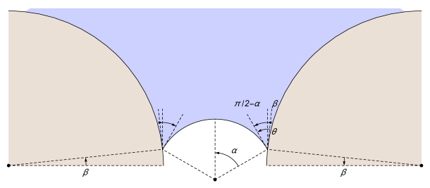
Figure 12: Detail of the refence configuration $\mathcal{B}^{0}$ of the RVE; the domain occupied by the liquid is parametrized by the three non-independent angles $\alpha$, $\beta$ and $\theta$.

For the sake of convenience the circumferential interfaces between the liquid and the wet air are labeled as North (N), East (E), South (S) and West (W)-Arch, respectively, turning clockwise from the North.

Due to the displacement of the beads centers, given by equation (49)the centers of the E-Arch and the W-Arch are displaced in the direction of the gradient of $J$. Their curvatures change so as to keep constant the contact angle $\theta$ at the junction line, and in particular the curvature of the E-Arch decreases, as it is pulled out of the intergranular space, whilst that of the W-Arch increases, as it is pushed inwards it. Notice that some liquid must be ejected from the pore chamber so as to make consistent the placement of the W-Arch with the requirement of displacing the liquid to the boundary of the RVE, keeping fixed the contact angle, see Figure 5. Finally in order to guarantee a constant value of the ratio between the amount of liquid (in volume) and the volume of the pore space, say of the degree of saturation, the N-Arch and the S-Arch are displaced and rotated keeping their curvatures almost constant during the deformation process.

Thus the problem of finding out the current placement of the liquid particles can be formulated as follows: given the third order tensor $\mathbb{A}$ determine the $\beta$-angles relative to the N-Arch, the E-Arch and the W-Arch as well as the value of the spherical part of the macro-scale deformation gradient, $a$, so that the saturation degree remains constant during deformation and the amount (in volume) of liquid initially trapped within the beads equals the amount (in volume) of the displaced liquid. Apparently in order to force the liquid to squeeze out of the pore chamber, a negative value of $a$ should be obtained.

Appendix D

Following the microporomechanics approach summarized by [48] the macro-scale gradient of $G_{li}$ is calculated starting from the definition of $G_{li}$ as the apparent average of $G^{\textrm{m}}_{li}$ relative to the liquid phase, see equation (51)₂; consequently on has:

$$G_{li,k}=\dfrac{\partial}{\partial X_{k}}\displaystyle\int\!f(Z-X)\,H^{0}_{liq}(Z)\,G^{\textrm{m}}_{li}(Z),$$ (D.1)

where $f(Z)$ is a $C^{\infty}$ function defined, at the micro-scale, on the entire Euclidean space of positions, which is equal to zero outside the reference configuration of the RVE, and is normalized so that its integral over the entire space is equal to one. The integral in equation (D.1) is calculated with respect to $Z$ variables. In equations (50)-(51) this function has been assumed to tend to the characteristic function of $\mathcal{B}^{0}$ divided by its volume. Finally $H^{0}_{liq}(Z)$ is the characteristic function of the liquid, in the reference configuration of the solid, which is also defined on the entire space of positions.

According with the definition of derivatives in the sense of distributions, the following chain of equalities hold true:

$$\begin{array}[]{rl}G_{li,k}&=-\displaystyle\int\!\dfrac{\partial f(Z-X)}{\partial Z_{k}}\,H^{0}_{liq}(Z)\,G^{\textrm{m}}_{li}(Z)=\displaystyle\int\!f(Z-X)\dfrac{\partial}{\partial Z_{k}}\left[H^{0}_{liq}(Z)\,G^{\textrm{m}}_{li}(Z)\right]=\vskip 6.0pt plus 2.0pt minus 2.0pt\\ &=\,\,\,\,\displaystyle\int\!f(Z-X)\,H^{0}_{liq}(Z)\,\dfrac{\partial}{\partial Z_{k}}G^{\textrm{m}}_{li}(Z)+\displaystyle\int\!f(Z-X)\,G^{\textrm{m}}_{li}(Z)\,\dfrac{\partial}{\partial Z_{k}}H^{0}_{liq}(Z)=\vskip 6.0pt plus 2.0pt minus 2.0pt\\ &=\,\,\,\,\left|\mathcal{B}^{0}\right|^{-1}\left(\displaystyle\int_{\mathcal{D}^{0}_{liq}\cap\mathcal{B}^{0}}\dfrac{\partial}{\partial Z_{k}}G^{\textrm{m}}_{li}(Z)\right)-\displaystyle\int_{\mathcal{D}^{0}_{liq}}\dfrac{\partial}{\partial Z_{k}}\left[f(Z-X)G^{\textrm{m}}_{li}(Z)\right]=\vskip 6.0pt plus 2.0pt minus 2.0pt\\ &=\,\,\,\,\left|\mathcal{B}^{0}\right|^{-1}\left(\displaystyle\int_{\partial(\mathcal{D}^{0}_{liq}\cap\mathcal{B}^{0})}G^{\textrm{m}}_{li}(Z)n_{k}\right)-\displaystyle\int_{\partial\mathcal{D}^{0}_{liq}}f(Z-X)G^{\textrm{m}}_{li}(Z)n_{k}=\vskip 6.0pt plus 2.0pt minus 2.0pt\\ &=\,\,\,\,\left|\mathcal{B}^{0}\right|^{-1}\left(\displaystyle\int_{\partial(\mathcal{D}^{0}_{liq}\cap\mathcal{B}^{0})}G^{\textrm{m}}_{li}(Z)n_{k}-\displaystyle\int_{\partial\mathcal{D}^{0}_{liq}\cap\mathcal{B}^{0}}G^{\textrm{m}}_{li}(Z)n_{k}\right)=\left|\mathcal{B}^{0}\right|^{-1}\left(\displaystyle\int_{\partial(\mathcal{D}^{0}_{liq}\cap\mathcal{B}^{0})\backslash\mathcal{I}^{0}_{f}}G^{\textrm{m}}_{li}(Z)n_{k}\right),\end{array}$$ (D.2)

where $\mathcal{I}^{0}_{f}$ is the interface between the liquid and the grain and the liquid and the gas within the reference configuration of the RVE, so that $\partial(\mathcal{D}^{0}_{liq}\cap\mathcal{B}^{0})\backslash\mathcal{I}^{0}_{f}$ represents that part of the liquid, pulled-back into the reference configuration of the solid, which overlaps the boundary of the reference configuration itself. $\left|\mathcal{B}^{0}\right|$ is the volume of the reference configuration of the RVE.

According with equation (D.2), even if a complete statement of the displacement of the liquid is not explicitly formulated, the macroscopic gradient of the liquid content $\phi S_{r}$ can be deduced from the micro-scale, assuming a suitable form of the gradient of $g^{\mathrm{m}}$ only over $\partial(\mathcal{D}^{0}_{liq}\cap\mathcal{B}^{0})\backslash\mathcal{I}^{0}_{f}$. Let the RVE be that of the left panel of Figure 5, the only part of the boundary of $\mathcal{B}_{0}$ which provides a non-vanishing contribution to $G_{li,k}$, and therefore to $(\phi S_{r})_{,k}$ is the right intergranular channel, which means that one only needs an instance on how the map $g^{\mathrm{m}}$ transforms a thin neighborhood of this part of the boundary into the corresponding domain of the initial configuration of the liquid.

References

References

- Alonso et al. [1990] E.E. Alonso, A. Gens, and A. Josa. A constitutive model for partially saturated soils. Géotechnique, 40(3):405–430, 1990.
- Alonso et al. [1999] E.E. Alonso, J. Vaunat, and A. Gens. Modelling the mechanical behaviour of expansive clays. Engineering Geology, 54(1):173–183, 1999.
- Alonso et al. [2010] E.E. Alonso, J.M. Pereira, J. Vaunat, and S. Olivella. A microstructurally based effective stress for unsaturated soils. Géotechnique, 60(12):913–925, 2010.
- Andò et al. [2012a] E. Andò, S.A. Hall, G. Viggiani, J. Desrues, and P. Bésuelle. Grain-scale experimental investigation of localised deformation in sand: A discrete particle tracking approach. Acta Geotechnica, 7(1):1–13, 2012a.
- Andò et al. [2012b] E. Andò, S.A. Hall, G. Viggiani, J. Desrues, and P. Bésuelle. Experimental micromechanics: Grain-scale observation of sand deformation. Geotechnique Letters, 2(7-9):107–112, 2012b.
- Bear [1972] J. Bear. Dynamics of Fluids in Porous Media. Elsevier, 1972.
- Biot [1972] M.A. Biot. Theory of finite deformations of porous solids. Indiana University Mathematics Journal, 21(7):597–620, 1972.
- Borja et al. [2013] R.I. Borja, X. Song, and W. Wu. Critical state plasticity. Part VII: Triggering a shear band in variably saturated porous media. Computer Methods in Applied Mechanics and Engineering, 261–262(0):66–82, 2013.
- Bourdin et al. [2000] B. Bourdin, G. Francfort, and J.J. Marigo. Numerical experiments in revised brittle fracture. Journal of the Mechanics and Physics of Solids, 48:797–826, 2000.
- Bourdin et al. [2012] B. Bourdin, C.P. Chukwudozie, and K. Yoshioka. A variational approach to the numerical simulation of hydraulic fracturing. In SPE Annual Technical Conference and Exhibition, SPE 159154. Society of Petroleum Engineers, 2012.
- Boyer and Lapuerta [2006] F. Boyer and C. Lapuerta. Study of a three component Cahn–Hilliard flow model. ESAIM: Mathematical Modelling and Numerical Analysis, 40:653–687, 2006.
- Boyer et al. [2010] F. Boyer, C. Lapuerta, S. Minjeaud, B. Piar, and M. Quintard. Cahn–Hilliard/Navier–Stokes model for the simulation of three-phase flows. Transport in Porous Media, 82(3):463–483, 2010.
- Brooks and Corey [1964] R. Brooks and A. Corey. Hydraulic properties of porous media. Colorado State University Hydrology Papers No. 3, 1964.
- Buckingham [1907] E. Buckingham. Studies on the movement of soil moisture. Bulletin 38. USDA Bureau of Soils, Washington, DC, 1907.
- Buscarnera and Einav [2012] G. Buscarnera and I. Einav. The yielding of brittle unsaturated granular soils. Géotechnique, 62(2):147–160, 2012.
- Cahn and Hilliard [1958] J.W. Cahn and J.E. Hilliard. Free energy of nonuniform system: I. Interfacial free energy. The Journal of Chemical Physics, 28(2):258–267, 1958.
- Cahn [1959] J.W. Cahn. Free energy of nonuniform system: II. Thermodynamic basis. The Journal of Chemical Physics, 30(5):1121–1124, 1959.
- Cahn and Hilliard [1959] J.W. Cahn and J.E. Hilliard. Free energy of nonuniform system: III. Nucleation in a two-component incompressible fluid. The Journal of Chemical Physics, 31(3):688–699, 1959.
- Casini [2012] F Casini. Deformation induced by wetting: a simple model. Canadian Geotechnical Journal, 49(8):954–960, 2012.
- Chambon et al. [2001] R. Chambon, D. Caillerie, and T. Matsuchima. Plastic continuum with microstructure, local second gradient theories for geomaterials: localization studies. International Journal of Solids and Structures, 38(46–47):8503 – 8527, 2001.
- [21] E.N.M. Cirillo, N. Ianiro, and G. Sciarra. Solid-fluid segregation in saturated porous media. In Poromechanics IV - 4th Biot Conference on Poromechanics, pages 929–934, 2009.
- Cirillo et al. [2010] E.N.M. Cirillo, N. Ianiro, and G. Sciarra. Phase coexistence in consolidating porous media. Physical Review E, 81(6):061121, 2010.
- Cirillo et al. [2011] E.N.M. Cirillo, N. Ianiro, and G. Sciarra. Phase transition in saturated porous media: Pore-fluid segregation in consolidation. Physica D: Nonlinear Phenomena, 240(17):1345–1351, 2011.
- Cirillo et al. [2012] E.N.M. Cirillo, N. Ianiro, and G. Sciarra. Kink localization under asymmetric double-well potentials. Physical Review E, 86(4):041111, 2012.
- Cirillo et al. [2013] E.N.M. Cirillo, N. Ianiro, and G. Sciarra. Allen–Cahn and Cahn–Hilliard-like equations for dissipative dynamics of saturated porous media. Journal of the Mechanics and Physics of Solids, 61(2):629–651, 2013.
- Collin et al. [2006] F. Collin, R. Chambon, and R. Charlier. A finite element method for poro-mechanical modelling of geotechnical problems using local second gradient models. International Journal for Numerical Methods in Engineering, 65(11):1749–1772, 2006.
- Collins [2005] I.F. Collins. The concept of stored plastic work or frozen elastic energy in soil mechanics. Geotechnique, 55(5):373–382, 2005.
- Costanza-Robinson et al. [2011] M.S. Costanza-Robinson, B.D. Estabrook, and D.F. Fouhey. Representative elementary volume estimation for porosity, moisture saturation, and air-water interfacial areas in unsaturated porous media: Data quality implications. Water Resources Research, 47(7):W07513, 2011.
- Coussy [2004] O. Coussy. Poromechanics. John Wiley & Sons, Ltd, 2004.
- Coussy [2010] O. Coussy. Mechanics and Physics of Porous Solids. John Wiley & Sons, Ltd, 2010.
- Coussy et al. [2004] O Coussy, Dangla P, T Lassabatère, and V Baroghel-Bouny. The equivalent pore pressure and the swelling and shrinkage of cement-based materials. Materials and Structures, 37(1):15–20, 2004.
- Coussy et al. [2010] O. Coussy, J.-M. Pereira, and J. Vaunat. Revisiting the thermodynamics of hardening plasticity for unsaturated soils. Computers and Geotechnics, 37(1):207–215, 2010.
- Cueto-Felgueroso and Juanes [2009a] L. Cueto-Felgueroso and R. Juanes. A phase field model of unsaturated flow. Water Resources Research, 45(10):W10409, 2009a.
- Cueto-Felgueroso and Juanes [2010] L. Cueto-Felgueroso and R. Juanes. Reply to comment by David A. DiCarlo on ”A phase field model of unsaturated flow”. Water Resources Research, 46(12):W12802, 2010.
- Cueto-Felgueroso and Juanes [2012] L. Cueto-Felgueroso and R. Juanes. Macroscopic phase-field model of partial wetting: bubbles in a capillary tube. Physical Review Letters, 108:144502, 2012.
- Cueto-Felgueroso and Juanes [2014] L. Cueto-Felgueroso and R. Juanes. A phase-field model of two-phase Hele-Shaw flow. Journal of Fluid Mechanics, 758:522–552, 2014.
- Cueto-Felgueroso and Juanes [2008] L. Cueto-Felgueroso and R. Juanes. Nonlocal interface dynamics and pattern formation in gravity-driven unsaturated flow through porous media. Physical Review Letters, 101(24):244504, 2008.
- Cueto-Felgueroso and Juanes [2009b] L. Cueto-Felgueroso and R. Juanes. Stability analysis of a phase-field model of gravity-driven unsaturated flow through porous media. Physical Review E, 79(3):036301, 2009b.
- Culligan et al. [2004] K.A. Culligan, D. Wildenschild, B.S.B. Christensen, W.G. Gray, M.L. Rivers, and A.F.B. Tompson. Interfacial area measurements for unsaturated flow through a porous medium. Water Resources Research, 40(12):W12413, 2004.
- Dalla et al. [2002] E. Dalla, M. Hilpert, and C.T. Miller. Computation of the interfacial area for two-fluid porous medium systems. Journal of Contaminant Hydrology, 56(1):25–48, 2002.
- de Gennes [1985] P.G. de Gennes. Wetting: statics and dynamics. Reviews of Modern Physics, 57(3):827–863, 1985.
- Dell’Isola et al. [2003] F. Dell’Isola, G. Sciarra, and R.C. Batra. Static deformations of a linear elastic porous body filled with an inviscid fluid. Journal of Elasticity, 72(1-3):99–120, 2003.
- Dell’Isola et al. [2009] F. Dell’Isola, G. Sciarra, and S. Vidoli. Generalized Hooke’s law for isotropic second gradient materials. Proceedings of the Royal Society A, 465(2107):2177–2196, 2009.
- Desrues and Andò [2015] J. Desrues and E. Andò. Strain localisation in granular media. Comptes Rendus Physique, 16(1):26–36, 2015.
- Desrues and Viggiani [2004] J. Desrues and G. Viggiani. Strain localization in sand: An overview of the experimental results obtained in Grenoble using stereophotogrammetry. International Journal for Numerical and Analytical Methods in Geomechanics, 28(4):279–321, 2004.
- Desrues et al. [1985] J. Desrues, J. Lanier, and P. Stutz. Localization of the deformation in tests on sand sample. Engineering Fracture Mechanics, 21(4):909–921, 1985.
- DiCarlo et al. [2008] D.A. DiCarlo, R. Juanes, T. LaForce, and T.P. Witelski. Nonmonotonic traveling wave solutions of infiltration into porous media. Water Resources Research, 44(2):W02406, 2008.
- Dormieux et al. [2006] L. Dormieux, D. Kondo, and F.-J. Ulm. Microporomechanics. John Wiley & Sons, 2006.
- Francfort and Marigo [1998] G. Francfort and J.J. Marigo. Revisiting brittle fracture as an energy minimization problem. Journal of the Mechanics and Physics of Solids, 46(8):1319–1342, 1998.
- Gens et al. [2006] A. Gens, M. Sánchez, and D. Sheng. On constitutive modelling of unsaturated soils. Acta Geotechnica, 1(3):137–147, 2006.
- Germain [1973] P. Germain. La méthode des puissances virtuelles en mécanique des milieux continus. I. Théorie du second gradient. Journal de Mécanique, 12:235–274, 1973.
- Gomez and Hughes [2011] H. Gomez and T.J.R. Hughes. Provably unconditionally stable, second-order time-accurate, mixed variational methods for phase-field models. Journal of Computational Physics, 230(13):5310–5327, 2011.
- Gomez et al. [2013] H. Gomez, L. Cueto-Felgueroso, and R. Juanes. Three-dimensional simulation of unstable gravity-driven infiltration of water into a porous medium. Journal of Computational Physics, 238:217–239, 2013.
- Gray and Hassanizadeh [1989] W.G. Gray and S.M. Hassanizadeh. Averaging theorems and averaged equations for transport of interface properties in multiphase systems. International Journal of Multiphase Flow, 15(1):81–95, 1989.
- Gray and Schrefler [2001] W.G. Gray and B.A. Schrefler. Thermodynamic approach to effective stress in partially saturated porous media. European Journal of Mechanics - A/Solids, 20(4):521 – 538, 2001.
- Gray et al. [2009] W.G. Gray, B.A. Schrefler, and F. Pesavento. The solid phase stress tensor in porous media mechanics and the hill–mandel condition. Journal of the Mechanics and Physics of Solids, 57(3):539–554, 2009.
- Hall et al. [2010] S.A. Hall, M. Bornert, J. Desrues, Y. Pannier, N. Lenoir, G. Viggiani, and P. Bésuelle. Discrete and continuum analysis of localised deformation in sand using x-ray CT and volumetric digital image correlation. Géotechnique, 60(5):315–322, 2010.
- Hassanizadeh and Gray [1990] S.M. Hassanizadeh and W.G. Gray. Mechanics and thermodynamics of multiphase flow in porous media including interphase boundaries. Advances in Water Resources, 13(4):169–186, 1990.
- Hassanizadeh and Gray [1993] S.M. Hassanizadeh and W.G. Gray. Toward an improved description of the physics of two-phase flow. Advances in Water Resources, 16:53–67, 1993.
- Hassanizadeh et al. [2002] S.M. Hassanizadeh, M.A. Celia, and H.K. Dahle. Dynamic effect in the capillary pressure–saturation relationship and its impacts on unsaturated flow. Vadose Zone Journal, 1(1):38–57, 2002.
- Houlsby [1997] GT Houlsby. The work input to an unsaturated granular material. Géotechnique, 47(1):193–196, 1997.
- Jacqmin [2000] D. Jacqmin. Contact-line dynamics of a diffuse fluid interface. Journal of Fluid Mechanics, 402:57–88, 2000.
- Jamet et al. [2001] D. Jamet, O. Lebaigue, N. Coutris, and J.M. Delhaye. The second gradient method for the direct numerical simulation of liquid–vapor flows with phase change. Journal of Computational Physics, 169(2):624–651, 2001.
- Joekar-Niasar et al. [2010] V. Joekar-Niasar, M. Prodanović, D. Wildenschild, and S.M. Hassanizadeh. Network model investigation of interfacial area, capillary pressure and saturation relationships in granular porous media. Water Resources Research, 46(6), 2010.
- Jommi [2000] C. Jommi. Remarks on the constitutive modelling of unsaturated soils. In Tarantino, A. and Mancuso, C., editor, Experimental Evidence and Theoretical Approaches in Unsaturated Soils, pages 139–153, 2000. ISBN 90-5809-186-4. International Workshop on Unsaturated Soils, TRENT, ITALY, APR 10-12, 2000.
- Kim [2012] J. Kim. Phase-field models for multi-component fluid flows. Commun. Comput. Phys, 12(3):613–661, 2012.
- Lamorgese et al. [2011] A.G. Lamorgese, D. Molin, and R. Mauri. Phase field approach to multiphase flow modeling. Milan Journal of Mathematics, 79(2):597–642, 2011.
- Lenoir et al. [2007] N. Lenoir, M. Bornert, J. Desrues, P. Bésuelle, and G. Viggiani. Volumetric digital image correlation applied to x-ray microtomography images from triaxial compression tests on argillaceous rock. Strain, 43(3):193–205, 2007.
- Leverett [1940] MC Leverett. Capillary behavior in porous solids. Trans. Am. Inst. Min. Eng., 142:341–358, 1941.
- Lewis and Schrefler [1998] R.W. Lewis and B.A. Schrefler. The Finite Element Method in the Deformation and Consolidation of Porous Media. John Wiley & Sons, Ltd, 1998.
- Lowengrub and Truskinovsky [1998] J. Lowengrub and L Truskinovsky. Quasi–incompressible Cahn–Hilliard fluids and topological transitions. Proceedings of the Royal Society of London. Series A: Mathematical, Physical and Engineering Sciences, 454(1978):2617–2654, 1998.
- Marle [1982] C.M. Marle. On macroscopic equations governing multiphase flow with diffusion and chemical reactions in porous media. International Journal Engng. Sci., 20 (5):647–662, 1982.
- Matsushima et al. [2002] T. Matsushima, R. Chambon, and D. Caillerie. Large strain finite element analysis of a local second gradient model: application to localization. International Journal for Numerical Methods in Engineering, 54(4):499–521, 2002.
- Mindlin [1964] R.D. Mindlin. Micro-structure in linear elasticity. Archive of Rational Mechanics and Analysis, 16:51–78, 1964.
- Morrow [1970] N.R. Morrow. Physics and thermodynamics of capillary action in porous media. Industrial & Engineering Chemistry, 62(6):32–56, 1970.
- Niessner and Hassanizadeh [2008] J. Niessner and S.M. Hassanizadeh. A model for two-phase flow in porous media including fluid-fluid interfacial area. Water Resources Research, 44(8), 2008.
- Nikooee et al. [2013] E. Nikooee, G. Habibagahi, S.M. Hassanizadeh, and A. Ghahramani. Effective stress in unsaturated soils: A thermodynamic approach based on the interfacial energy and hydromechanical coupling. Transport in Porous Media, 96(2):369–396, 2013.
- Olivella et al. [1996] S. Olivella, A. Gens, J. Carrera, and E.E. Alonso. Numerical formulation for a simulator (Code_Bright) for the coupled analysis of saline media. Engineering Computations, 13(7):87–112, 1996.
- Papatzacos [2002] P. Papatzacos. Macroscopic two-phase flow in porous media assuming the diffuse-interface model at pore level. Transport in Porous Media, 49(2):139–174, 2002.
- Papatzacos and Skjoeveland [2004] P. Papatzacos and S.M. Skjoeveland. Relative permeability from thermodynamics. SPE Journal, 9(1):47–56, 2004.
- Reeves and Celia [1996] P.C. Reeves and M.A. Celia. A functional relationship between capillary pressure, saturation, and interfacial area as revealed by a pore-scale network model. Water Resources Research, 32(8):2345–2358, 1996.
- Richards [1931] L.A. Richards. Capillary conduction of liquids through porous mediums. Journal of Applied Physics, 1(5):318–333, 1931.
- Rotisciani et al. [2014] G. Rotisciani, G. Sciarra, A. Desideri, and F. Casini. Modeling rainfall infiltration through coarse and fine-grained unsaturated geomaterials. In 6th International conference on unsaturated soils, UNSAT 2014, pages 521–528. Taylor & Francis Group, 2014.
- Rotisciani et al. [2015] G.M. Rotisciani, G. Sciarra, F. Casini, and A. Desideri. Hydro-mechanical response of collapsible soils under different infiltration events. International Journal for Numerical and Analytical Methods in Geomechanics, 39(11):1212–1234, 2015.
- Sanavia et al. [2002] L. Sanavia, B.A. Schrefler, and P. Steinmann. A formulation for an unsaturated porous medium undergoing large inelastic strains. Computational Mechanics, 28(2):137–151, 2002.
- Sanavia et al. [2006] L. Sanavia, F. Pesavento, and B.A. Schrefler. Finite element analysis of non-isothermal multiphase geomaterials with application to strain localization simulation. Computational Mechanics, 37(4):331–348, 2006.
- Sciarra [2013] G. Sciarra. Strain-gradient poromechanical description of unsaturated porous materials. In Poromechanics V - Proceedings of the 5th Biot Conference on Poromechanics, pages 1255–1264, 2013.
- Sciarra et al. [2007] G. Sciarra, F. dell’Isola, and O. Coussy. Second gradient poromechanics. International Journal of Solids and Structures, 44:6607–6629, 2007.
- Sciarra et al. [2008] G. Sciarra, F. dell’Isola, N. Ianiro, and A. Madeo. A variational deduction of second gradient poroelasticity: Part I: General theory. Journal of Mechanics of Materials and Structures, 3 (3):507–526, 2008.
- Seppecher [1989] P. Seppecher. Étude des conditions aux limites en théorie du second gradient: cas de la capillarité. C. R. Acad. Sci. Paris Sér. II Méc. Phys. Chim. Sci. Univers Sci. Terre, 309(6):497–502, 1989.
- Seppecher [1996] P. Seppecher. Moving contact lines in the Cahn-Hilliard theory. Int. J. Engng. Sci., 34(9):977–992, 1996.
- Sieffert et al. [2009] Y. Sieffert, S. Al Holo, and R. Chambon. Loss of uniqueness of numerical solutions of the borehole problem modelled with enhanced media. International Journal of Solids and Structures, 46(17):3173–3197, 2009.
- Song and Borja [2014] X. Song and R.I. Borja. Mathematical framework for unsaturated flow in the finite deformation range. International Journal for Numerical Methods in Engineering, 97(9):658–682, 2014.
- Sulem and Vardoulakis [2004] J. Sulem and I.G. Vardoulakis. Bifurcation Analysis in Geomechanics. CRC Press, 2004.
- Tamagnini [2004] R. Tamagnini. An extended cam-clay model for unsaturated soils with hydraulic hysteresis. Géotechnique, 54(3):223–228, 2004.
- Toupin [1962] R.A. Toupin. Elastic materials with couple-stresses. Archive of Rational Mechanics and Analysis, 11:385–414, 1962.
- van Genuchten [1980] M. Th. van Genuchten. A closed-form equation for predicting the hydraulic conductivity of unsaturated soils. Soil Science Society of America Journal, 44:892–898, 1980.
- Vardoulakis et al. [1978] I. Vardoulakis, M. Goldscheider, and G. Gudehus. Formation of shear bands in sand bodies as a bifurcation problem. International Journal for Numerical and Analytical Methods in Geomechanics, 2(2):99–128, 1978.