TI tether rig for solving secular spinrate change problem of electric sail

Abstract

The electric solar wind sail (E-sail) is a way to propel a spacecraft by using the natural solar wind as a thrust source. The problem of secular spinrate change was identified earlier which is due to the orbital Coriolis effect and tends to slowly increase or decrease the sail’s spinrate, depending on which way the sail is inclined with respect to the solar wind. Here we present an E-sail design and its associated control algorithm which enable spinrate control during propulsive flight by the E-sail effect itself. In the design, every other maintether (“T-tether”) is galvanically connected through the remote unit with the two adjacent auxtethers, while the other maintethers (“I-tethers”) are insulated from the tethers. This enables one to effectively control the maintether and auxtether voltages separately, which in turn enables spinrate control. We use a detailed numerical simulation to show that the algorithm can fully control the E-sail’s spin state in real solar wind. The simulation includes a simple and realistic set of controller sensors: an imager to detect remote unit angular positions and a vector accelerometer. The imager resolution requirement is modest and the accelerometer noise requirement is feasible to achieve. The TI tether rig enables building E-sails that are able to control their spin state fully and yet are actuated by pure tether voltage modulation from the main spacecraft and requiring no functionalities from the remote units during flight.

url]http://www.electric-sailing.fi

Nomenclature

au	Astronomical unit, 149 597 871 km
$A$	Auxiliary factor
$\mathrm{clamp}\,(x,a,b)$	Clamp function, limitation of $x$ in $[a,b]$
$d_{\mathrm{max}}$	Maximum thrust reduction for $f_{4}$, 0.05
$dF/dz$	Thrust per unit length produced by tether
$\hat{\mathbf{e}}_{r}$	Radial unit vector
$f(t)$	Generic function of time $t$
$f_{1}(t),f_{2}(t),\tilde{f}(t)$	Gap filler functions
$f$	Total throttling factor
$f_{1},f_{2},f_{3}$	Individual throttling factors
$f_{4},f_{5}$	Throttling factors for oscillation damping
$f_{6}$	Throttling factor for setting thrust
$f_{6}^{\mathrm{max}}$	Maximum allowed $f_{6}$, 1.01
$f_{6}^{\mathrm{old}}$	Previous value of $f_{6}$
$\mathbf{F}$	Generic thrust vector
$F_{\mathrm{goal}}$	Goal E-sail thrust, 100 mN
$\mathbf{F}_{n}$	Spinplane normal component of thrust
$\mathbf{F}_{\mathrm{rig}}$	Thrust on tether rig
$\mathbf{F}_{s}$	Spinplane component of thrust
$\mathbf{F}_{\mathrm{sc}}$	Thrust on spacecraft
$\mathbf{F}_{\mathrm{tot}}$	Total thrust, $\mathbf{F}_{\mathrm{sc}}+\mathbf{F}_{\mathrm{rig}}$
$\mathbf{F}_{\mathrm{tot}}^{\mathrm{ave}}$	Time-averaged version of $\mathbf{F}_{\mathrm{tot}}$
$F_{0}$	Typical tether tension
$g$	Acceleration due to gravity, 9.81 m/s2
$g_{\mathrm{d}}$	Greediness factor for damping in $f_{4}$, 3.0
$g_{\mathrm{s}}$	Greediness factor for spinrate change, 2.0
$g_{\mathrm{t}}$	Greediness factor for spinplane turning, 1.0
$K$	Spin axis orientation keeper factor
$\mathbf{L}$	Angular momentum vector
$\mathbf{L}(0)$	Initial angular momentum vector
$m_{p}$	Proton mass
$m_{\mathrm{rig}}$	Mass of tether rig, 11 kg
$m_{\mathrm{sc}}$	Mass of spacecraft body, 300 kg
$m_{\mathrm{tot}}$	Total mass, 311 kg
$\max(a,b)$	Maximum of $a$ and $b$
$\min(a,b)$	Minimum of $a$ and $b$
$\hat{\mathbf{n}}_{\mathrm{goal}}$	Goal orientation unit vector of spin axis
$\hat{\mathbf{n}}_{\mathrm{SW}}$	Unit vector along (nominal) SW, (0,0,1)
$N_{\mathrm{w}}$	Number of tethers
$\mathbf{p}$	Momentum of tether rig
$P_{\mathrm{dyn}}^{\perp}$	Solar wind dynamic pressure due to tether-perpendicular flow
$\mathbf{r}$	Position of remote unit
$\hat{\mathbf{s}}$	Unit vector along spin axis
$S$	Spinrate increase factor
$t$	Time
$t_{1}$,$t_{2}$	Starttime and endtime of data gap
$\mathbf{v}$	Velocity of remote unit
$v_{\mathrm{s}}$	Spin axis aligned speed of remote units
$v_{\mathrm{tot}}$	Average rotation speed of remote units
$\mathbf{v}_{\perp}$	Tether-perpendicular component of solar wind velocity
$V_{0}$	Tether voltage
$V_{1}$	Voltage corresponding to solar wind proton kinetic energy
$x,y,z$	Cartesian coordinates in inertial frame
$x^{\prime}$,$y^{\prime}$,$z^{\prime}$	Spin axis aligned Cartesian coordinates
$\hat{\mathbf{x}}^{\prime},\hat{\mathbf{y}}^{\prime},\hat{\mathbf{z}}^{\prime}$	Unit vectors along $x^{\prime}$, $y^{\prime}$, $z^{\prime}$
$\alpha$	Sail angle, angle between SW and spin axis
$\Delta t$	Timestep how often controller is called, 2 s
$\Delta t_{\mathrm{d}}$	How often damper is called, 20 s
$\epsilon_{0}$	Vacuum permittivity
$\phi$	Polar angle of spin axis vector
$\rho$	Solar wind mass density
$\tau_{\mathrm{d5}}$,$\tau_{\mathrm{d6}}$	Timescale parameters, 1200 s
$\omega$	Angular frequency of the sail spin
$\Omega$	Angular frequency of heliocentric orbit

1 Introduction

The solar wind electric sail (E-sail) is a concept how to propel a spacecraft in the solar system using the natural solar wind (SW) [1, 2]. The E-sail uses a number of thin metallic and centrifugally stretched tethers which are biased at high positive potential (Fig. 1). The biasing is effected by an onboard electron gun which continuously pumps out negative charge from the tethers.

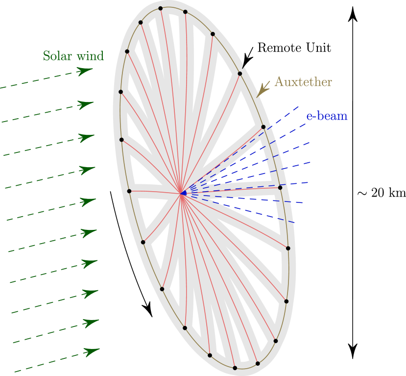
Figure 1: Schematic presentation of the E-sail.

Thrust vectoring can be done by turning the spin plane by differential modulation of the tether voltages in sync with the rotation [11]. In this way one can also generate a thrust component which is perpendicular to the solar wind so that one can e.g. spiral outward or inward in the solar system. The thrust magnitude can be throttled by reducing the voltage and current of the electron gun. Hence both thrust direction and magnitude can be controlled, which makes the E-sail a generic method for moving around in the solar system (outside Earth’s magnetosphere) without consuming propellant. For example, it was demonstrated numerically that one can reach Mars by the E-sail, even using a simple control law, despite persistent variations of the solar wind density and the solar wind flow velocity vector [11].

The following secular spinrate change problem was, however, identified [12]. When an E-sail orbits around the sun with the sail inclined with respect to the SW, the orbital Coriolis effect causes a secular increase or decrease of the spinrate. Inclining the sail is necessary if one wants to produce transverse thrust perpendicular to the SW direction, which is usually the case. Specifically, if the sail is inclined so that it brakes the orbital motion and keeps the spacecraft spiralling towards the sun, the spinrate decreases, and if the sail is inclined in the opposite way so that the orbit is an outward moving spiral, the spinrate increases. The rate of spinrate increase or decrease obeys approximately the equation [12]

$$\omega(t)\approx\omega(0)e^{\pm(\Omega\tan\alpha)t}.$$ (1)

Here $\Omega$ is the angular frequency of the heliocentric orbit and $\alpha$ is the sail angle, i.e. the (positive) angle between the sail spin axis and the SW direction. For example if $\alpha$ is $35^{\circ}$ and the spacecraft is in a circular orbit at 1 au distance, the spinrate changes by 9 % in each week. To overcome the problem, various technical solutions were proposed and analysed, for example the use of ionic liquid field-effect electric propulsion (FEEP) thrusters [8, 9, 7] or photonic blades [5] on the remote units.

In this paper we present a novel design concept (the TI tether rig) for the E-sail which overcomes the secular spinrate problem and yields a technically simple hardware. We also present a control algorithm and demonstrate by detailed numerical simulation that the algorithm is able to fly the E-sail in real SW with full capability to control the orientation of the spin plane and the spinrate. We also demonstrate that the algorithm is able to accomplish its task using a simple set of sensors (remote unit position imager and vector accelerometer) with realistic amount of measurement noise.

The structure of the paper is as follows. We show that electric auxtethers enable spinrate control, present the TI tether rig design, the control algorithm, the dynamical simulation model and the simulation results. The paper closes with summary and conclusions.

2 Electric auxtethers enable spinrate control

In E-sail plasma physics, a tether produces thrust per unit length which is approximately proportional to the flow velocity of the plasma (equation 3 of Janhunen et al. [2]):

$$\frac{dF}{dz}=0.18\max\left(0,V_{0}-V_{1}\right)\sqrt{\epsilon_{0}P_{\mathrm{dyn}}^{\perp}}.$$ (2)

Here $V_{1}=(1/2)m_{p}v_{\perp}^{2}/e\approx 1\,$kV is voltage corresponding to solar wind proton kinetic energy, $V_{0}$ is the tether voltage and $P_{\mathrm{dyn}}^{\perp}=\rho v_{\perp}^{2}$ is the solar wind dynamic pressure expressed in terms of the solar wind mass density $\rho$ and the solar wind tether-perpendicular velocity $\mathbf{v}_{\perp}$. More accurate and more complicated thrust formulas also exist [2], but the assumption that the tether-parallel velocity causes no propulsive effect remains exact as long as the tether is much longer than the radius of the electron sheath that surrounds the tether so that end effects can be ignored. This condition is typically well valid since the tether length is of order 10-20 km while the sheath radius at 1 au is $\sim 0.1$ km. In this section, the only thing that we need from E-sail plasma physics is that a tether segment generates a thrust vector which is aligned with the segment-perpendicular component of the solar wind flow.

We consider an E-sail as in Fig. 2 where the auxiliary tethers (auxtethers) are metallic and can be biased at high voltage, similarly to the maintethers. A segment of an auxtether then generates E-sail thrust which is perpendicular to it. Our aim is then to show that if the auxtether voltages can be controlled independently from the maintether voltages, spinrate control becomes possible.

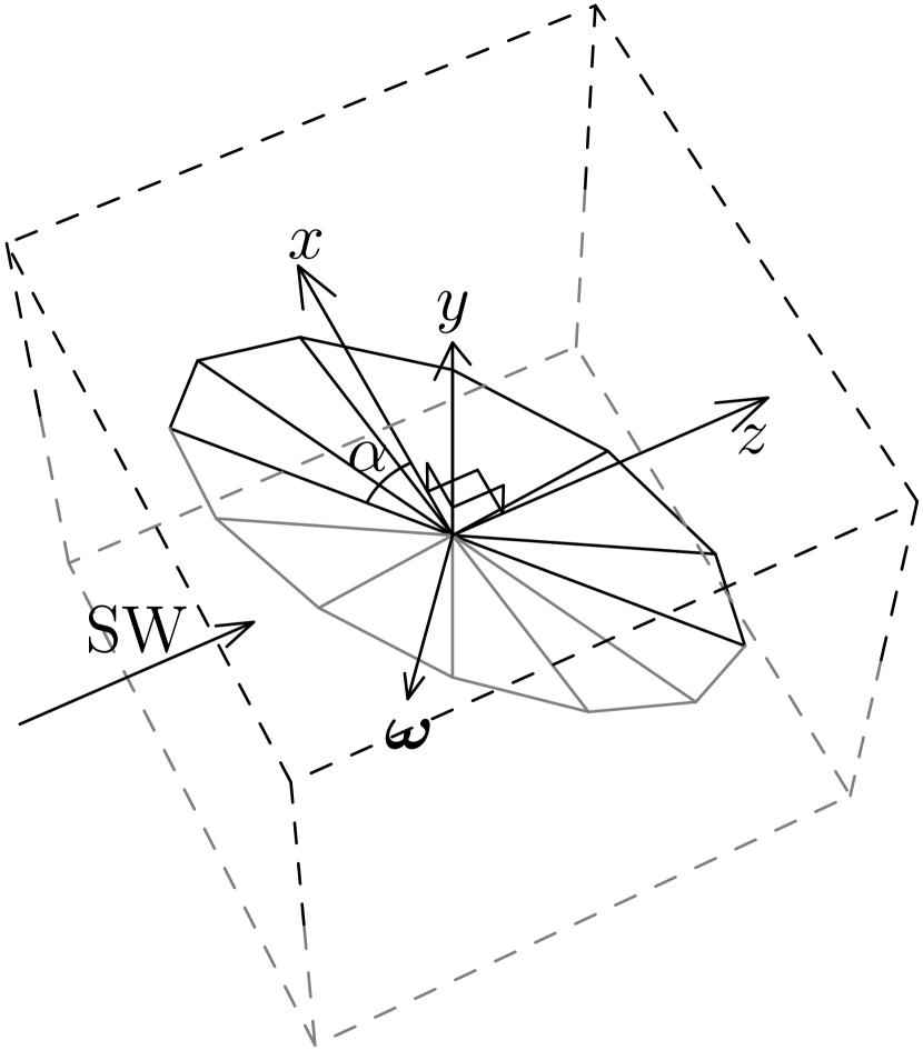
Figure 2: Three-dimensional schematic presentation of spinning planar E-sail inclined at angle $\alpha$ with respect to SW flow ($\alpha$ lies in the $xz$ plane). Lines below $y=0$ plane are drawn in greyscale to ease visualisation. The $z$ coordinate is along the SW.

Figure 3a again shows an E-sail inclined at angle $\alpha$ to the SW flow, but now viewed from the top, antiparallel to the $y$ axis. Consider a maintether in the $xz$ plane i.e. in the plane of Fig. 3a. The maintether generates a thrust vector $\mathbf{F}$ which is perpendicular to itself.

Figure 3: E-sail force components. (a) Maintether in $xz$ plane, (b) maintether parallel to $y$, (c) maintether parallel to $y$ plus auxtether segment.

Figure 3b shows the same maintether $90^{\circ}$ rotation later when it is parallel to $y$ axis. Now, because the tether is perpendicular to the SW, its thrust vector $\mathbf{F}$ is aligned with the SW. We decompose $\mathbf{F}$ in spinplane component $\mathbf{F}_{s}$ and spinplane normal component $\mathbf{F}_{n}$. The spinplane component $\mathbf{F}_{s}$ brakes the tether’s spinrate when it moves upstream and accelerates it $180^{\circ}$ rotation later, and the net effect vanishes. This means that by modulating maintether voltages alone, one cannot change the sail’s spinrate if one wants to keep the sail’s orientation constant. Modulation of maintether voltages can tilt the sail which also changes the spinrate, but independent control of the spinrate and orientation is not possible if maintether modulation is the only available control. The secular spinrate change effect arises because when orbiting the Sun, the Sun moves with respect to the inertial frame (the celestial sphere defined by distant stars) and the sail must track this motion. Doing so requires application of torque because in the absence of torque the angular momentum vector of the sail tends to be conserved i.e. the spin axis tends to point to the same distant star. Tracking the Sun’s motion is equivalent to continuous turning of the sail, which changes the spinrate as a byproduct if performed by modulating the maintether voltages. The spinrate change occurs in this case because in order to tilt the sail, the maintethers must be modulated unsymmetrically in the $y$ direction so that symmetry in their upstream/downstream motion is broken and a net spinrate change results. For an equivalent explanation in the Sun-pointing orbital reference frame, see Figure 8 of [12].

Panel 3c is the same as panel 3b, but we have added a charged auxtether segment at the tip of the maintether. The thrust vector $\mathbf{F}$ is now a vector sum of the maintether thrust and the auxtether thrust. The maintether thrust is still along the SW flow as it was in 3b, but the auxtether’s thrust contribution is perpendicular to the auxtether, i.e. perpendicular to the spin plane. As a result, $\mathbf{F}$ is not aligned with the SW and the ratio $F_{s}/F_{n}$ depends on the ratio of the auxtether thrust versus the maintether thrust. In particular, by modulating the auxtether and maintether voltages separately, the ratio $F_{s}/F_{n}$ can be different when the maintether is parallel or antiparallel with the $y$ axis. By having the same $F_{n}$ but different $F_{s}$ in the upstream and downstream portions of the maintether’s rotation cycle, we can modify the sail’s spinrate while keeping its orientation fixed. Separate control of sail spinrate and spinplane orientation becomes possible because one has two control parameters in each angular segment, namely maintether voltage and auxtether voltage.

3 TI tether rig

To enable separate control of auxtether and maintether voltages, one could use various technical means, for example, each remote unit could carry a potentiometer or other means of regulating the auxtether voltage between zero and the maintether voltage. However, we propose a simpler arrangement where the remote units need no active parts. We propose that even-numbered maintethers are such that their remote unit is galvanically connected with both the left-side and right-side auxtethers (Fig. 4, blue), while odd-numbered maintethers are electrically insulated from the remote unit (Fig. 4, red). We call the even-numbered tethers the T-tethers because of the T-shaped shape of the blue equipotential region, and odd-numbered tethers are correspondingly called I-tethers.

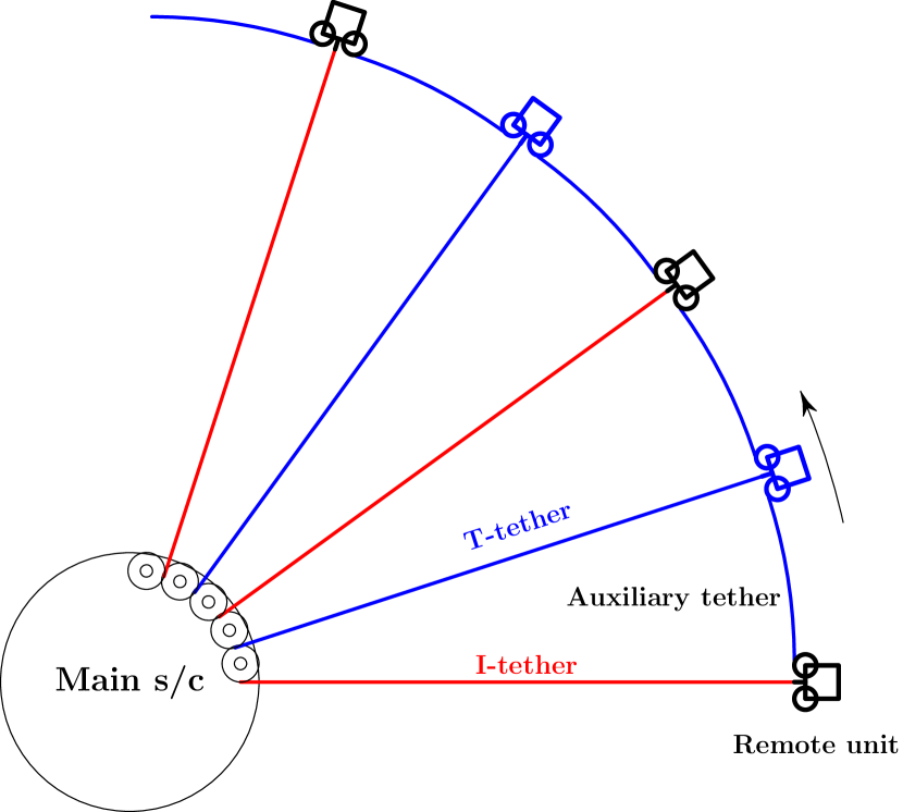
Figure 4: Schematic presentation of the TI tether rig.

In a given angular sector of the sail, we can effectively increase (decrease) the auxtether voltages by setting T-tethers to higher (lower) voltage than I-tethers. The auxtethers are always at the same potential as their associated T-tether so that no potentiometers or other functional parts are needed on the remote units. Two types of remote units are needed: ones that provide galvanic connection between the maintether and the two auxtethers, and ones that provide an insulating connection between all three connecting tethers. As usual, the remote units contain reels of the auxtethers which are used during deployment phase. During propulsive flight, no functionality is required from the remote units. The units only have to continue to provide the mechanical and electrical connection which is of galvanic and insulating type of even and odd-numbered units, respectively. Because of the presence of T-tethers and I-tethers, we call the design as a whole the TI tether rig.

4 Control algorithm

The control algorithm consists of six throttling factors which are multiplied together at the end (Eq. 17) to yield the time-dependent voltage throttling factor for each maintether. The six factors and their qualitative roles are introduced in Table 1.

Table 1: The six throttling factors.

$f_{1}$	Turning the spinplane
$f_{2}$	Maintaining the spinplane
$f_{3}$	Changing the spinrate
$f_{4}$	Damping collective oscillations
$f_{5}$	Damping oscillations of tethers
$f_{6}$	Setting thrust to wanted value

Before defining the six throttling factors, we discuss some preliminaries related to the general strategy of the control algorithm. Let $\mathbf{r}=(x,y,z)$ be the remote unit’s position vector relative to the spacecraft and $\hat{\mathbf{e}}_{r}=\mathbf{r}/r$ is the corresponding unit vector. We denote the angular momentum of the tether rig by $\mathbf{L}$ and the corresponding unit vector (spin axis vector) by $\hat{\mathbf{s}}=\mathbf{L}/L$. The controller computes an instantaneous angular momentum $\mathbf{L}_{\mathrm{inst}}$ approximately from imaged positions $\mathrm{r}$ of the remote units and their velocities $\mathrm{v}$ found by finite differencing with $\Delta t=2$ s timestep. The angular momentum $\mathbf{L}$ used by the control algorithm below is a time-averaged version of $\mathbf{L}_{\mathrm{inst}}$ which is obtained by continuously solving the differential equation

$$\frac{d\mathbf{L}}{dt}=\frac{\mathbf{L}_{\mathrm{inst}}-\mathbf{L}}{\tau_{\mathrm{L}}}$$ (3)

where $\tau_{\mathrm{L}}=1200$ s is the timescale used in the time-averaging.

We are now ready to give the detailed definitions of the six throttling factors used by the control algorithm.

4.1 Factor $f_{1}$

The first throttling factor is

$$f_{1}=\max\left[0,1-g_{\mathrm{t}}\hat{\mathbf{e}}_{r}\cdot\left(\hat{\mathbf{s}}\times\hat{\mathbf{n}}_{\mathrm{goal}}\right)\right]$$ (4)

where $g_{\mathrm{t}}=1.0$ is a greediness parameter for spinplane turning and $\hat{\mathbf{n}}_{\mathrm{goal}}$ is the goal spin axis orientation. The factor $f_{1}$ is responsible for turning the spinplane when $\hat{\mathbf{s}}\neq\hat{\mathbf{n}}_{\mathrm{goal}}$. It modulates the tether voltages so that the SW thrust applies a torque to the tether rig.

4.2 Factor $f_{2}$

The second throttling factor $f_{2}$ takes care of keeping the spinplane orientation constant. The second factor is

$$f_{2}=(1-A)K+A$$ (5)

where the ’spinplane keeper factor’ $K$ is

$$K=\frac{1}{|\hat{\mathbf{n}}_{\mathrm{SW}}-\hat{\mathbf{e}}_{r}(\hat{\mathbf{e}}_{r}\cdot\hat{\mathbf{n}}_{\mathrm{SW}})|^{2}}$$ (6)

and the auxiliary factor

$$A=\frac{1}{1+N_{\mathrm{w}}/(2\pi)}.$$ (7)

The algorithm works moderately well also with $A=0$, but by numerical experimentation we found that it works better if $A$ is computed from Eq. (7). The denominator of $K$ is the tether-perpendicular component of $\hat{\mathbf{n}}_{\mathrm{SW}}$. If the tethers spin rapidly so that they move nearly in a plane without coning, $K$ does not depend on tether phase angle. However, in a real sail some coning occurs. Then the $K$ factor decreases and increases thrust on the upwind and downwind orientations of the spinning tether, respectively, to keep the total torque zero.

4.3 Factor $f_{3}$

The third throttling factor $f_{3}$ takes care of increasing or decreasing the spinrate. First we define the spinrate increase factor $S$ by

$$S=g_{\mathrm{s}}\left[s_{\mathrm{goal}}-\frac{|\mathbf{L}|}{|\mathbf{L}(0)|}\right].$$ (8)

Here $g_{\mathrm{s}}=2.0$ is the spinrate increase greediness factor and $s_{\mathrm{goal}}$ is the goal for the relative spinrate, i.e. the angular mometum magnitude relative to the initial angular momentum magnitude $|\mathbf{L}(0)|$. The throttling factor is given by

$$f_{3}=1-\mathrm{clamp}\,\left(\pm S\hat{\mathbf{v}}\cdot\hat{\mathbf{n}}_{\mathrm{SW}},-c_{\mathrm{st}},c_{\mathrm{st}}\right).$$ (9)

Here $\mathbf{v}$ is the instantaneous velocity of the remote unit (relative to the spacecraft, similarly to $\mathrm{r}$) and $c_{\mathrm{st}}=0.2$ is the maximum allowed amplitude of our sawtooth tether modulation. Plus sign is selected for T-tethers and minus sign for I-tethers. The function $\mathrm{clamp}$ forces the first argument within given limits $a$ and $b$, $a\leq b$. For any $x$, $\mathrm{clamp}\,(x)$ is defined by

$$\mathrm{clamp}\,(x,a,b)=\max(a,\min(x,b))$$ (10)

The controller algorithm as described up to now works, but it does not damp tether oscillations that are produced by SW variations and the spinplane manoeuvres. Neither does it set the E-sail thrust to a wanted value. The purpose of the remaining factors $f_{4}$, $f_{5}$ and $f_{6}$ is to take care of these.

4.4 Factor $f_{4}$

For the first damping related factor, $f_{4}$, we measure the spin-axis aligned speed $v_{\mathrm{s}}$ (sign convention: positive sunward) of the remote units relative to the spacecraft, averaged over the remote units. The measurement is done by finite differencing the imaged remote unit angular positions and the throttling factor is

$$f_{4}=1+\min\left(0,g_{\mathrm{d}}\frac{v_{\mathrm{s}}}{v_{\mathrm{tot}}}\right)$$ (11)

where $g_{\mathrm{d}}=3.0$ is greediness factor for damping and $v_{\mathrm{tot}}$ is the average rotation speed of the remote units with respect to the spacecraft. The idea is that if the tether rig oscillates collectively along the spin axis so that the tether cone angle changes periodically, the oscillation is damped if voltages are slightly throttled down when the rig is moving in the direction of the SW.

4.5 Factor $f_{5}$

The factor $f_{4}$ reduces collective oscillation of the whole tether rig, but each tether can also oscillate individually like a guitar string between the spacecraft and the remote unit. For reducing these a bit faster oscillations we introduce throttling factor $f_{5}$. We measure the instantaneous thrust force $\mathbf{F}_{\mathrm{sc}}$ acting on the spacecraft body (at 20 s resolution) by an onboard vector accelerometer. Notice that $\mathbf{F}_{\mathrm{sc}}$ is the force exerted on the spacecraft by the tethers which is usually not equal to the total E-sail force exerted on the whole tether rig, except as an average over a long enough time period. When $|\mathbf{F}_{\mathrm{sc}}|$ increases significantly, we apply overall throttling $f_{5}$ to tether voltages where

$$f_{5}=1-\mathrm{clamp}\,\left(\tau_{\mathrm{d5}}\frac{1}{F_{0}}\frac{d|\mathbf{F}_{\mathrm{sc}}|}{dt},0,d_{\mathrm{max}}.\right)$$ (12)

Here $\tau_{\mathrm{d5}}=1200$ s is a damping timescale parameter, $d_{\mathrm{max}}=0.05$ is the maximum applied thrust reduction due to damping and $F_{0}$ is the typical tether tension multiplied by the number of tethers $N_{\mathrm{w}}$. We set the typical tension equal to the tether tension in the initial state.

4.6 Factor $f_{6}$

The final throttling factor $f_{6}$ is used to settle the E-sail thrust to a wanted value $F_{\mathrm{goal}}$. We estimate the E-sail thrust on the tether rig by using the inertial coordinate frame equation

$$\mathbf{F}_{\mathrm{rig}}=\frac{d\mathbf{p}}{dt}+\frac{m_{\mathrm{rig}}}{m_{\mathrm{sc}}}\mathbf{F}_{\mathrm{sc}}$$ (13)

where $\mathbf{p}$ is the momentum of the tether rig relative to the spacecraft (determined by imaging and finite differencing the remote unit angular positions), $m_{\mathrm{rig}}$ is the mass of the tether rig and $m_{\mathrm{sc}}$ is the mass of the spacecraft body. The first term is due to acceleration of the tether rig with respect to the spacecraft body and the second term is due to acceleration of the spacecraft with respect to an inertial frame of reference. The time average of the first term is obviously zero, but its instantaneous value is usually nonzero and it carries information about tether rig oscillations that we want to damp. The instantaneous thrust exerted on the whole system (spacecraft plus tether rig) is

$$\mathbf{F}_{\mathrm{tot}}=\mathbf{F}_{\mathrm{sc}}+\mathbf{F}_{\mathrm{rig}}.$$ (14)

From the instantaneous $\mathbf{F}_{\mathrm{tot}}$ we calculate a time-averaged version $\mathbf{F}_{\mathrm{tot}}^{\mathrm{ave}}$ by keeping on solving the time-dependent differential equation

$$\frac{d\mathbf{F}_{\mathrm{tot}}^{\mathrm{ave}}}{dt}=\frac{\mathbf{F}_{\mathrm{tot}}-\mathbf{F}_{\mathrm{tot}}^{\mathrm{ave}}}{\tau_{\mathrm{d6}}}$$ (15)

where $\tau_{\mathrm{d6}}=1200$ s is another damping timescale parameter. Finally the overall throttling factor $f_{6}$ is calculated as

$$f_{6}=\mathrm{clamp}\,\left(f_{6}^{\mathrm{old}}+\frac{\Delta t_{\mathrm{d}}}{\tau_{\mathrm{d6}}}\frac{F_{\mathrm{goal}}-|\mathbf{F}_{\mathrm{tot}}^{\mathrm{ave}}|}{F_{\mathrm{goal}}},0,f_{6}^{\mathrm{max}}\right)$$ (16)

where $\Delta t_{\mathrm{d}}=20$ s is the timestep how often the damping algorithm is called, $f_{6}^{\mathrm{old}}$ is the previous value of $f_{6}$ and $f_{6}^{\mathrm{max}}=1.01$ is $f_{6}$’s maximum allowed value. Equation (16) resembles solving a differential equation similar to (3) and (15), except that (16) also clamps the solution if it goes outside bounds $(0,f_{6}^{\mathrm{max}})$.

4.7 Combining the throttling factors

The total throttling factor is

$$f=\frac{f_{1}f_{2}f_{3}}{\max(f_{1}f_{2}f_{3})}f_{4}f_{5}\min(1,f_{6}).$$ (17)

where the maximum is taken over the maintethers.

Factors $f_{4}$, $f_{5}$ and $f_{6}$ are updated at $\Delta t_{\mathrm{d}}=20$ s intervals while $f_{1}$, $f_{2}$ and $f_{3}$ are updated with $\Delta t=2$ s time resolution. The motivation for using slower updating of $f_{4}$, $f_{5}$ and $f_{6}$ is only to save onboard computing power. The computing power requirement is low in any case, but as a matter of principle we want to avoid unnecessary onboard computing cycles.

Factors $f_{4}$ and $f_{5}$ make only small modifications to the total throttling factor $f$. Despite this, their ability to damp tether rig oscillations is profound.

The tether voltages are modulated by $f$. We assume in this paper that the E-sail force depends linearly on $V$ so that we can achieve the wanted force throttling by simply modulating the voltages by $f$. This should be a rather good approximation (see equation 3 of Janhunen et al. [2]). Were this assumption not made, the nonlinear relationship, if any, should be modelled or determined experimentally and then used during flight to map thrust modulation values $f$ into voltage modulation values. Doing so is straightforward if such relationship is known. Hence there is no loss of generality in making a working assumption of a linear relationship between voltage and thrust.

5 Simulation model

We use a dynamical simulator which was built for simulating dynamical behaviour of the E-sail tether rig [3, 4]. The simulator models the E-sail as a collection of point masses, rigid bodies and interaction forces between them. Also external forces and torques can be included. The core of the simulator solves the ordinary differential equations corresponding to Newton’s laws for the collection the bodies. The solver is an eight order accurate adaptive Runge-Kutta solver adapted from Press et al. [10]. The solver provides in practice fully accurate discretisation in time. The only essential approximation is replacing continuous tethers by chains of point masses connected by interaction forces that model their elasticity. The E-sail force (a more accurate version of Eq. 2 taken from Janhunen et al. [2]) is included in the model. Table 2 summarises the main parameters of the simulation used in this paper.

Table 2: Simulation parameters.

Number of tethers $N_{\mathrm{w}}$	20
Tether length	10 km
Thrust goal $F_{\mathrm{goal}}$	100 mN
Solar distance	1 au
Baseline tether voltage	20 kV
Maximum tether voltage	40 kV
Spacecraft body mass $m_{\mathrm{sc}}$	300 kg
Remote unit mass	0.4 kg
Initial tether tension	5 cN
Initial spin period	2000 s
Tether linear mass density	$1.1\cdot 10^{-5}$ kg/m
Tether parallel wires	$3\times\phi{=}20\,\mu$m
Tether wire Young modulus	100 GPa
Tether wire relative loss modulus	0.03
Remote unit imager resolution	$0.17^{\circ}$
Onboard accelerometer noise	1.5 $\mu g/\sqrt{\mathrm{Hz}}$
Synthetic SW density	7.3 cm-3
Synthetic SW speed	400 km/s
Number of tether discr. points	10
Placement of discretisation points	Parabolic
Number of auxtether discr. points	1
Simulation length	3 days

The core of the simulator coded in C++ for high performance, while the definition of the model (the collection of point masses, rigid bodies, their interaction forces and external forces and torques) is coded in Lua scripting language. One Lua function implements the control algorithm described in Section 4 above. The control algorithm needs only two types of sensors. Firstly, we need imaging sensors to detect the angular positions of the remote units with moderate angular $0.17^{\circ}$ resolution and 2 s temporal resolution. The angular resolution requirement corresponds to about 2200$\times$530 pixels, either in a single panoramic imager or several small imagers along the spacecraft’s perimeter. Secondly, we need a vector accelerometer onboard the main spacecraft, for which we assume noise level of 1.5 $\mu g/\sqrt{\mathrm{Hz}}$. A low-noise low-noise accelerometer such as Colibrys SF-1500 has noise level five times smaller than this. The imager resolution and accelerometer noise level were found by numerical experimentation. The chosen values are optimal in the sense that smaller measurement error in sensors would not noticeably improve the fidelity of the control and its oscillation damping properties.

In Table 3 we summarise the parameters of the control algorithm, including its virtual sensors.

Table 3: Default parameters of the control algorithm and its virtual sensors.

$d_{\mathrm{max}}$	Maximum thrust reduction for $f_{4}$	0.05
$f_{6}^{\mathrm{max}}$	Maximum allowed $f_{6}$	1.01
$F_{\mathrm{goal}}$	Goal E-sail thrust	100 mN
$g_{\mathrm{d}}$	Greediness for damping in $f_{4}$	3.0
$g_{\mathrm{s}}$	Greediness for spinrate change	2.0
$g_{\mathrm{t}}$	Greediness for spinplane turning	1.0
$\Delta t$	Controller call interval	2 s
$\Delta t_{\mathrm{d}}$	Damper call interval	20 s
$\tau_{\mathrm{d5}}$	Timescale for damping oscillations	1200 s
$\tau_{\mathrm{d6}}$	Timescale for regulating thrust	1200 s
$\tau_{\mathrm{L}}$	Ang. momentum averaging time	1200 s

6 Simulation results

All simulations start from an initial state where the sail rotates perpendicular to the SW. Synthetic constant SW is used in first three runs. In the last run, real SW is used. In all runs the thrust is modulated by $1-\exp(-t/(4\mathrm{h}))$ so that it starts off gradually from zero (a smooth transition from zero to one in a 4-hour timescale). This is done to avoid inducing tether oscillations as an initial transient: although the algorithm can damp such oscillations, damping would not occur immediately.

In Run 1 (Fig. 5), the tilt angle goal (panel a) is zero until 0.5 days, then it is set to 45^∘ where it remains for 1.5 days. The sail starts turning when the angle is set and reaches almost $45^{\circ}$ angle after 0.75 days. Then the $\phi$ angle goal (the polar angle of the spin vector) is changed from 90^∘ to -90^∘ so that the sail starts turning again, via zero to the opposite direction. At 2 days the $\alpha$ angle goal is returned back to zero. Thus, Run 1 exercises a back and forth swing of the tether rig. Spinrate regulation greediness parameter $g_{\mathrm{s}}$ is set to zero in Run 1 so that we can observe the natural tendency of the spinrate to vary during the turning manoeuvre. The spinrate (Fig. 5, panel d) increases up to 25 % from the initial value when the sail reaches $\approx 45^{\circ}$ angle. The increase is due to conservation of the sun-directed angular momentum component $L_{z}$: $|\mathbf{L}|=\sqrt{L_{x}^{2}+L_{y}^{2}+L_{z}^{2}}$ must increase if $L_{x}^{2}+L_{y}^{2}$ increases while $L_{z}$ remains constant.

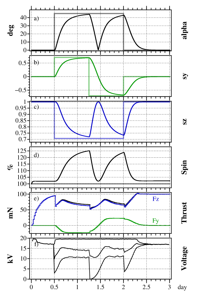
Figure 5: Result of Run 1. (a) angle $\alpha$ between SW and spin axis; (b) $\hat{\mathbf{s}}_{y}$ ($y$ component of spin axis unit vector $\hat{\mathbf{s}}$); (c) $\hat{\mathbf{s}}_{z}$ ($z$ component of $\hat{\mathbf{s}}$); (d) spin angular momentum relative to initial angular momentum in percent; (e) thrust along SW (blue, $F_{z}$), perpendicular to it (green, $F_{y}$) and total (black); (f) tether instantaneous minimum, mean and maximum voltages. In a-d, thicker grey and pastel lines show the commanded goal of each parameter.

The thrust direction (Fig. 5, panel e) varies according to the spinplane orientation. The total thrust is somewhat smaller when the spinplane is actively turned, which is due to the fact some tethers are then throttled in voltage (Fig. 5, panel f).

In Run 2 (Fig. 6), the goal $\alpha$ angle is put to $35^{\circ}$ throughout. The spinrate control greediness parameter $g_{\mathrm{d}}$ is put to its normal value of 2.0. The spinrate goal is 110 % spin for the first 0.75 days and is put to very large value after that. The controller turns the spinplane smoothly to $35^{\circ}$ which also increases the spinrate moderately because of $L_{z}$ conservation. When the spinrate goal is put high, the spinrate starts to increase almost linearly, reaching 60 % increase at the end of the run which is 2.25 days since setting the spinrate goal high. As a byproduct of the spinrate increase part of the algorithm, the sail angle (Fig. 6, panel a) decreases slightly from $35^{\circ}$ to about $30^{\circ}$. The reason is that the spinrate modification and tilt angle modification parts of the controller algorithm slightly compete with each other because both use the same tether voltages for actuation. We do not expect this competition to be a practical issue because usually (to compensate the secular trend) the wanted spinrate change is much slower than in Run 2. In any case, Run 2 shows that if needed for any reason, the spinrate can be increased in a matter of few days with the model sail.

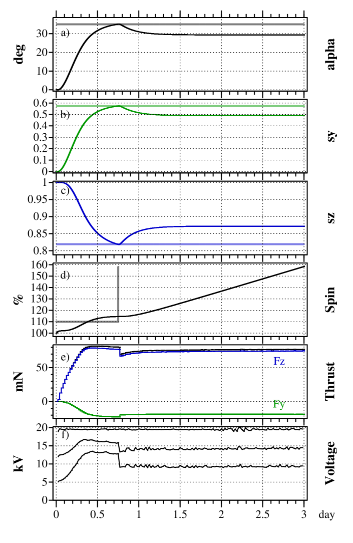
Figure 6: Same as Fig. 5 but for Run 2: demonstration of rapid spin increase.

Run 3 (Fig. 7) is similar to Run 2, but now we demonstrate decreasing rather than increaseing of the spinrate. The spinrate goal is put to 40 % at 0.75 days. The spin slows down obediently. In this case the sail angle increases somewhat above the goal value $35^{\circ}$.

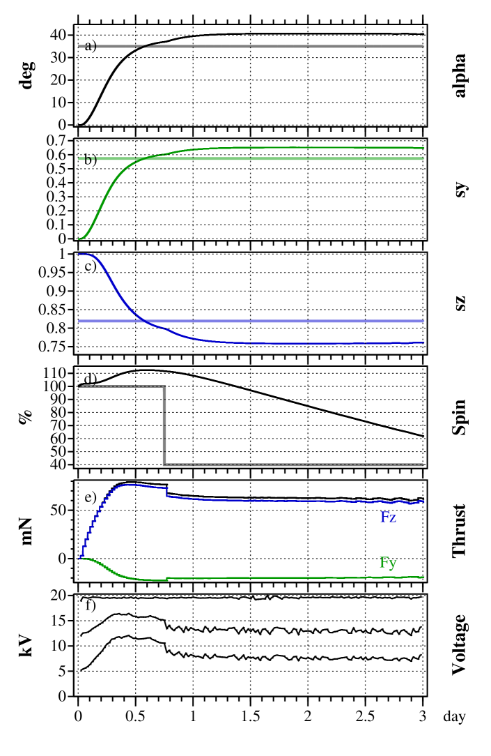
Figure 7: Same as Fig. 5 but for Run 3: demonstration of spin decrease.

Finally, in Run 4 (Fig. 8) we simulate a typical use case of the E-sail. We set the sail angle $\alpha$ goal to $35^{\circ}$ and the spinrate goal at 100 %. In Run 4 we also use real SW data to drive the E-sail where $t=0$ corresponds to epoch January 1, 2000, 00:00 UT. The used SW data comes from NASA/GSFCV’s OMNI 1-minute resolution dataset through OMNIWeb (Fig. 9,[6]).

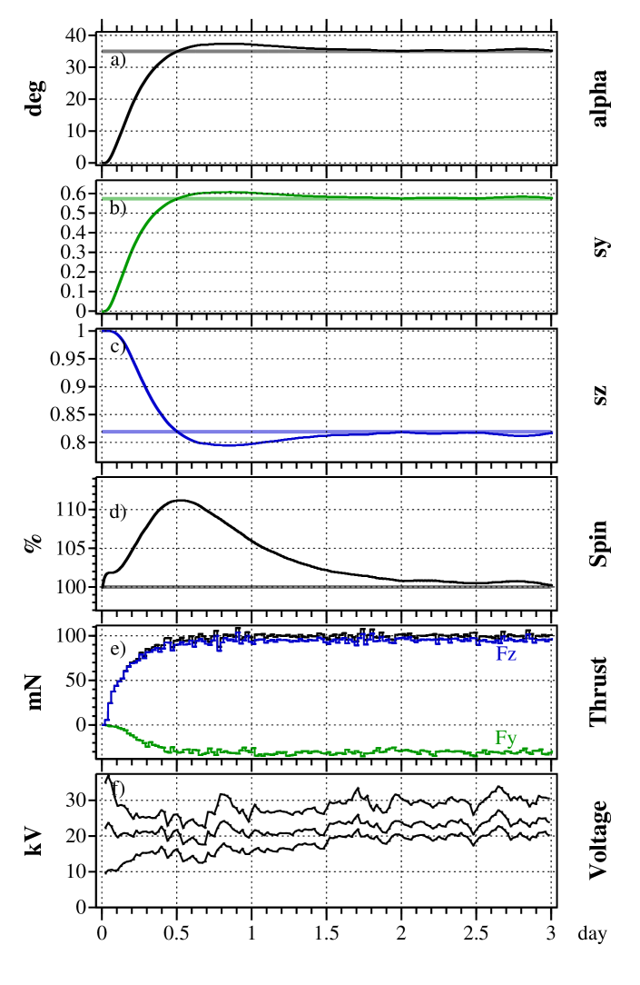
Figure 8: Same as Fig. 5 but for Run 4: typical use case of E-sail with real SW.

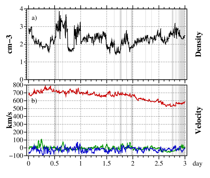
Figure 9: SW data used in Run 4 (Fig. 8). (a) plasma density, (b) SW velocity components (blue $x$, green $y$, red $z$). Filled data gaps are shown as grey.

The OMNI dataset contains data gaps, which we filled by the following simple algorithm (Fig. 10). Let $f(t)$ be the data which has a gap at $t_{1}{<}t{<}t_{2}$. Mirror the data before $t_{1}$ to make a function $f_{1}(t)=f(2t_{1}-t)$. Now, function $f_{1}(t)$ fills the gap $[t_{1},t_{2}]$ with data that has the same spectral content as the real data $f(t)|t{<}t_{1}$. The filler $f_{1}(t)$ has, however, a discontinuity where the gap ends at $t_{2}$ and we return to real data $f(t)|t{>}t_{2}$. To remedy this, we carry out a similar procedure at the other end, mirroring data around $t_{2}$ to get $f_{2}(t)=f(2t_{2}-t)$. Finally we construct the filler $\tilde{f}(t)$, $t_{1}{<}t{<}t_{2}$, by linear interpolation between $f_{1}(t)$ and $f_{2}(t)$: $\tilde{f}(t)=(1-u)f_{1}(t)+uf_{2}(t)$ where $u=(t-t_{1})/(t_{2}-t_{1})$. The result is a gap-free solar wind time series that has no discontinuous jumps and that retains as much as possible the spectral properties of the true data.

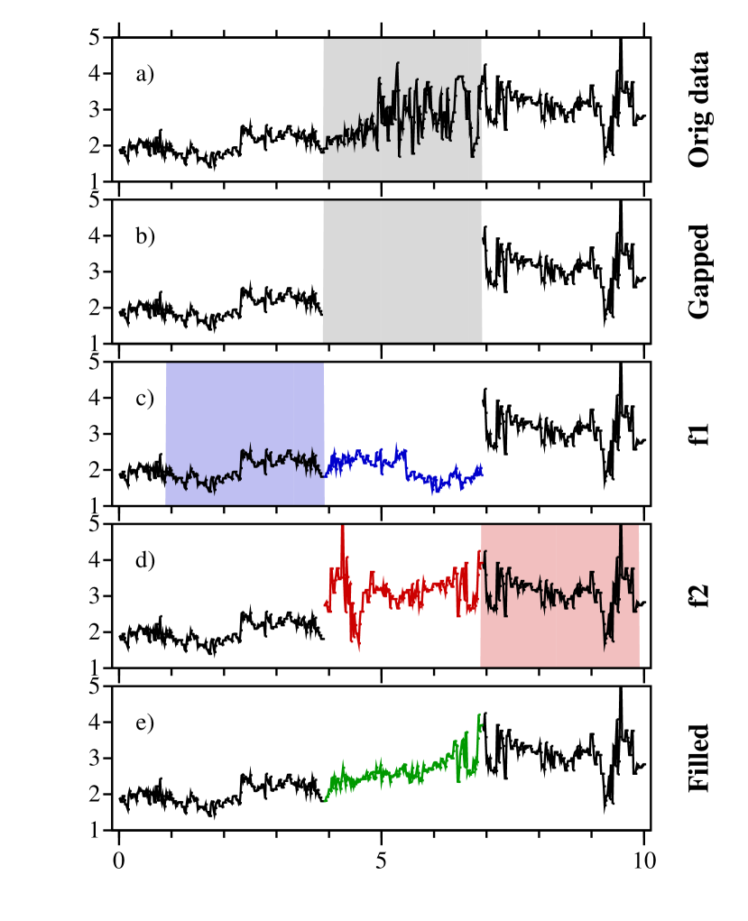
Figure 10: SW data gap filling algorithm. (a) original data, (b) original data with gap removed, (c) gap filled by mirroring left side function, (d) gap filled by mirroring right side function, (e) linear interpolation of c and d removes jumps at gap boundaries. The data shown in all panels is the solar wind plasma density in units of $\mathrm{cm}^{-3}$.

Run 4 demonstrates numerically that the control algorithm correctly tilts the sail to the wanted tilt angle and keeps it there, despite variations of the solar wind. Tilting the sail causes the spinrate to increase initially by $\sim 10$ % because of angular momentum conservation, but the control algorithm later settles it back to the commanded value. The algorithm accomplishes these tasks by using only the two types of simulated sensors (with realistic noise components) described in Section 5.

7 Summary and conclusions

We have presented a new E-sail design and its accompanying control algorithm and sensor set which satisfies the following requirements:

1. Control of tether voltages from the main spacecraft is the only actuation mechanism.

2. Capability to control the orientation of the spin plane and thereby the orientation of the E-sail thrust vector.

3. Delivery of the wanted amount of E-sail thrust.

4. Spinrate acceleration and deceleration capability. With typical parameters, the spinrate modification control authority is many times larger than what is needed to overcome the heliocentric orbit Coriolis effect.

5. Remote units have no functionality requirements after deployment.

6. Both maintethers and auxtethers are biased and thereby propulsive.

7. Only two sensors are needed: remote unit angular position detection by imaging and accelerometer.

8. Moderate resolution sufficies for the imaging sensors.

9. The accelerometer should have low noise ($<1.5\mu g/\sqrt{\mathrm{Hz}}$), but devices exist (e.g. Colibrys SF-1500) whose noise level is even five times less.

In the simulations of this paper we did not study deployment, but an obvious question is if the spinrate increase capability of the algorithm would be enough to deploy the sail in reasonable time. Based on our preliminary analysis, the answer seems to be yes, provided that deployment to a few hundred metre tether length is first achieved by some other means.

Another future work that could be performed with our simulation is systematic analysis of the average and maximum tether tension that occurs during the run. Although not reported here, we have already monitored tether tension in our simulations, and the version of the control algorithm presented in this paper (Table 3) was arrived at partly by trial and error minimisation of the occurring maximum tether tension when thrust was kept fixed. The peak tension is a measure of tether oscillations that the control algorithm tries to keep at bay, hence low peak tension is a figure of merit of the control algorithm. Typically the peak tension can become some tens of percent higher than the average tension.

We think that the TI tether rig is a significant step forward in E-sail design particularly because it enables full control of the angular momentum vector while not requiring any functionality from the remote units during flight. As a result, the secular spinrate problem originally identified by Toivanen and Janhunen [12] gets solved in a simple way.

8 Acknowledgement

The work was partly supported by the European Space Agency. We acknowledge use of NASA/GSFC’s Space Physics Data Facility’s OMNIWeb service and OMNI data.

References

- Janhunen [2004] P. Janhunen, Electric sail for spacecraft propulsion, J.Propuls.Power 20 (4) (2004) 763–764.
- Janhunen et al. [2010] P. Janhunen, et al., Electric solar wind sail: towards test missions, Rev.Sci.Instrum. 81 (2010) 111301.
- Janhunen [2013a] P. Janhunen, Description of E-sail dynamic simulator codes, Deliverable D51.1 of ESAIL FP-7 project, http://www.electric-sailing.fi/fp7/docs/D511.pdf, 2013 (accessed May 9, 2017).
- Janhunen [2013b] P. Janhunen, Report of performed runs, Deliverable D51.2 of ESAIL FP-7 project, http://www.electric-sailing.fi/fp7/docs/D51.2.pdf, 2013 (accessed May 9, 2017).
- Janhunen [2013c] P. Janhunen, Photonic spin control for solar wind electric sail, Acta Astronaut. 83 (2013) 85–90.
- King and Papitashvili [2005] J.H. King, N.E. Papitashvili, Solar wind spatial scales in and comparisons of hourly Wind and ACE plasma and magnetic field data, J.Geophys.Res. 110 (2005) A02104.
- Marcuccio et al. [2009] S. Marcuccio, N. Giusti, A. Tolstoguzov, Characterization of linear slit FEEP using an ionic liquid propellant, IEPC-09-180, Proc. 31th International Electric Propulsion Conference, Ann Arbor, MI (2009).
- Pergola et al. [2013] P. Pergola, N. Giusti, S. Marcuccio, Simplified FEEP test report, Deliverable D46.2 of ESAIL FP-7 project, http://www.electric-sailing.fi/fp7/docs/D462.pdf, 2013 (accessed May 9, 2017).
- Pergola et al. [2013] P. Pergola, N. Giusti, S. Marcuccio, Cost assessment for industrial product, Deliverable D46.3 of ESAIL FP-7 project, http://www.electric-sailing.fi/fp7/docs/D463.pdf, 2013 (accessed May 9, 2017).
- Press et al. [2007] W.H. Press, S.A. Teukolsky, W.T. Vetterling, B.P. Flannery, Numerical Recipes, third ed., Cambridge, 2007.
- [11] Toivanen, P.K and P. Janhunen, Electric sailing under observed solar wind conditions, Astrophys. Space Sci. Trans., 5 (2009) 61–69.
- Toivanen and Janhunen [2013] P.K. Toivanen, P. Janhunen, Spin plane control and thrust vectoring of electric solar wind sail by tether potential modulation, J.Propuls.Power 29 (2013) 178–185.