A Posterior Probability Approach for Gene Regulatory Network Inference in Genetic Perturbation Data

Abstract

Inferring gene regulatory networks is an important problem in systems biology. However, these networks can be hard to infer from experimental data because of the inherent variability in biological data as well as the large number of genes involved. We propose a fast, simple method for inferring regulatory relationships between genes from knockdown experiments in the NIH LINCS dataset by calculating posterior probabilities, incorporating prior information. We show that the method is able to find previously identified edges from TRANSFAC and JASPAR and discuss the merits and limitations of this approach.

Keywords: Bayesian inference, posterior probability, gene regulatory network, LINCS.

1 Introduction

Gene regulatory networks are very important in understanding the biological functioning of cells. Identifying the interactions between genes can aid biologists in their attempts to understand how the cell functions both in steady state and in reaction to external stimuli. Unfortunately, due to the complexity of the cells and the large number of genes involved, discovering the true networks is very difficult. In most cases the number of genes measured far exceeds the number of observations, as is typical in microarray or sequencing experiments. Any method for analyzing such data must take this fact into account. Often this is done by enforcing a sparsity constraint, either via an added penalty on non-sparseness or via priors placed on the model. Even with these constraints, the ability to make valid inference is limited in these high-dimensional regimes as the number of genes grows compared to the number of observations (Wainwright,, 2009; Verzelen,, 2012).

Many methods have been developed for inferring relationships between genes from gene expression data. One approach is to model the network holistically using Bayesian networks (Murphy et al.,, 1999; Kim et al.,, 2003, 2004; Zou and Conzen,, 2005; Lèbre et al.,, 2010; Scutari,, 2010). This yields good interpretability, but often does not scale well and is difficult to apply at the whole-genome level. Regression-based methods, where the expression level of a target gene is modeled as a function of the exression level of that gene’s regulators, can be applied to much larger sets of genes but lack the same overarching model of the entire network. Inference for these models generally becomes a statistical variable selection or model selection problem. Common methods for this include Significance Analysis of Microarrays (Tusher et al.,, 2001), Least Absolute Shrinkage and Selection Operator (LASSO) (Tibshirani,, 1996; Gustafsson et al.,, 2009; Menéndez et al.,, 2010) and Bayesian Model Averaging (BMA) (Raftery et al.,, 1997; Hoeting et al.,, 1999; Yeung et al.,, 2011; Lo et al.,, 2012; Young et al.,, 2014). Another class of methods looks at mutual information among the measured genes (Basso et al.,, 2005; Margolin et al.,, 2006; Faith et al.,, 2007; Meyer et al.,, 2007).

When looking for regulatory relationships, it has been found that the information available from knockout experiments, where a single gene is fully suppressed, can be highly informative since they give a way to identify a causal pathway, direct or indirect. In the DREAM4 in silico network challenge (http://wiki.c2b2.columbia.edu/dream/index.php?title=D4c2) (Marbach et al.,, 2009, 2010), the winning method used only the data from the knockout experiments to infer the true networks, ignoring the time-series data entirely (Pinna et al.,, 2010). In real biological experiments, full knockout experiments are not possible for many essential genes, but knockdown experiments, where the target gene is partially suppressed, are often available. Methods for analyzing knockdown or knockout data include correlation-based approaches (Salleh et al.,, 2015), implicit latent variable scoring (Yoo et al.,, 2002), and Bayesian network scoring (Friedman et al.,, 2000; Rogers and Girolami,, 2005; Fröhlich et al.,, 2007). In addition, there has been some work in combining steady-state data with knockdown data to improve results (Shojaie et al.,, 2014; Christley et al.,, 2009).

In this paper, we propose a simple, fast method for inferring gene regulatory relationships from just knockdown data. Our method uses a simple linear regression model focusing on single regulator-target gene pairs based on knockdown data. This method allows the incorporation of prior knowledge about the relationships and generates posterior probabilities which can be used to form a ranked edgelist or as a part of a more expansive analysis.

2 Data

Our data come from the National Institute of Health (NIH) Library of Integrated Network-based Cellular Signatures (LINCS) program (http://lincsproject.org/) (Duan et al.,, 2014). The aim of this program is to generate genetic and molecular signatures of cells in response to various perturbations. One thrust of this program is the large-scale generation of gene expression profiles using L1000 technology. This technology has resulted in measurements from over one million experiments to date on over fifty human cell lines. These cell lines are populations of cells descended from an original source cell and having the same genetic makeup, kept alive by growing them in a culture separate from their original source.

Each of the L1000 experiments measures the expression levels of 1000 landmark genes in the human genome. These genes were selected specifically to cover as much of the gene expression variation in cellular expression as possible, since all 20,000+ genes cannot be measured. These experiments have measured cellular response to more than 20,000 different chemical perturbagens. In addition, knockdown and over-expression experiments, where a single gene is targeted to control its expression level, have been performed on thousands of individual genes, both within and outside of the 1000 landmark genes.

The L1000 experiments were performed using Luminex Bead technology (Dunbar,, 2006), in which color-coded microspheres were coded to attach to specific RNA sequences corresponding to a landmark gene and fluoresce according to the level of that gene’s expression. Sets of beads for measuring the 1000 landmark genes were added to the solution for a single experiment along with the perturbing agent. The experiment was left for a specified period of time and then the gene expression levels were measured.

Experiments were done in sets on a single plate having individual wells for 384 experiments. This minimizes some external sources of error, such as environmental conditions, across these experiments. A small set of these experiments were used as controls with no perturbation. This gives a baseline distribution of expression level for each gene from which to measure deviations in other experiments. A common approach in this setup is to look at deviations in the perturbation experiments from the controls on the same plate, again recognizing that experiments on the same plate are likely to be more similar than those on different plates. Multiple plates, typically three or four, are prepared and analyzed together as a batch. These plates are prepared as technical replicates, with a given perturbation being prepared and then put into the same well of each plate. This gives additional power in removing systematic biases. Any given perturbation also is performed in multiple different batches, resulting in biological replicates since the sets of experiments were not prepared together.

3 Methods

We want to use the L1000 data to infer gene regulatory networks. This means that we need a method for inferring causality. One way to do this would be to use a causal time-series model, but the L1000 data include a very small number of time points (drug perturbation experiments include only one to two time points). Instead, we use knockdown experiments to identify a single gene as a putative causal agent. Although this limits the amount of information we can gain from a single experiment, it allows us to use a straightforward model with a clearly defined regulatory gene.

When looking at the knockdown experiments, it is important to understand that not all experiments are equally useful. The efficacy of the perturbation varies between target genes and even between experiments for the same target. The experimental setup of the LINCS data is helpful in identifying these differences. We use the control experiments on a plate to get an estimate of the normal variability of a gene. This eliminates some of the variability due to effects we cannot control or even measure, including differences in experimental conditions such as ambient temperature and the scientist performing the experiment, since these are captured in plate-level effects.

To take advantage of this aspect of the LINCS data, we calculate plate-level $z$-values for each gene in a knockdown experiment. To do this, we first calculate the baseline mean, $\bar{x}_{hp}$, and standard deviation, $s_{hp}$, for each gene $h$ across all control experiments on plate $p$. Then the $z$-value for gene $h$ in knockdown experiment $i$ on plate $p$ is

$$x^{*}_{hi}=\frac{x_{hi}-\bar{x}_{hp}}{s_{hp}}.$$

Once we have transformed the data in this way, we use a simple linear regression model to model the change in a target gene $t$ as dependent on the change in the knockdown gene $h$:

$$x^{*}_{ti} = \beta_{0}+\beta_{1}x^{*}_{hi}+\epsilon_{i},\leavevmode\nobreak\ \leavevmode\nobreak\ i=1,\dots,n_{h}$$ (1)

$$\epsilon_{i} \stackrel{{\scriptstyle\mbox{iid}}}{{\sim}} N(0,\sigma^{2}).$$ (2)

Here, $n_{h}$ is the number of available knockdown experiments for gene $h$. This model specifies a linear relationship between the $z$-score of the knockdown gene $h$ and that of the target gene $t$. This is a simplification of the true process underlying the relationship between genes $h$ and $t$, but it can still be effective for discovering relationships.

We estimate this model with a Bayesian approach using Zellner’s $g$-prior (Zellner,, 1986) for the model parameters $(\beta_{0},\beta_{1},\sigma^{2})$.

$$\beta_{1}|\sigma^{2},g \sim N\left(0,\frac{g\sigma^{2}}{\sum_{i}x^{*2}_{hi}}\right),$$

$$\Pr(\beta_{0},\sigma^{2}) \propto 1/\sigma^{2}.$$

The parameter $g$ specifies the expected size of the regression parameter $\beta_{1}$ relative to the standard error of the OLS estimate of $\beta_{1}$. The choice $g=1$ indicates that the regression parameter is expected to be nearly indistinguishable from the noise, and thus gives a lower bound for $g$. Also, $n_{h}/g$ is the effective number of data points in the prior, with $g=n_{h}$ corresponding to a unit information prior and giving similar results to BIC. We do not want a prior that has more spread than a unit information prior (Raftery,, 1999), and thus we choose $g$ in the range $1\leq g\leq n_{h}$. In this case, we used $g=\sqrt{n_{h}}$. We have found this to be a good compromise between the extremes. We found that when we estimated $g$ using an Expectation-Maximization algorithm (Dempster et al.,, 1977; Young et al.,, 2014), the estimated value was often close to $\sqrt{n_{h}}$.

The regression model with the $g$-prior allows us to quickly calculate the posterior probability that gene $h$ regulates gene $t$ (Christley et al.,, 2004). We first calculate the ratio of the likelihood that $h$ regulates $t$ given the data $\mathbf{x}$, $\Pr(h\rightarrow t|\mathbf{x})$, versus the likelihood that there is no regulatory relationship, $\Pr_{0}$. Further, we can incorporate a prior probability of regulation, $\pi_{ht}$, which reflects prior information regarding a regulatory relationship between genes $h$ and $t$. This gives us

$$T_{ht}\equiv\frac{\Pr(h\rightarrow t|\mathbf{x})}{\Pr_{0}}=\frac{\pi_{ht}}{1-\pi_{ht}}\exp\left[(n_{h}-2)\log(1+g)/2-(n_{h}-1)\log(1+g(1-R^{2}))/2\right],$$

where $R^{2}$ is the coefficient of determination for the simple linear regression model (1). From this we can get the posterior probability that $h$ regulates $t$, or posterior edge probability:

$$p_{ht}=\frac{\Pr(h\rightarrow t|\mathbf{x})}{\Pr(h\rightarrow t|\mathbf{x})+\Pr_{0}}=\frac{T_{ht}}{1+T_{ht}}.$$

We use this posterior edge probability to rank potential edges and find likely edges for further investigation.

Two advantages of this method are its speed and simplicity. To compute the z-scores, we first get plate-level means and standard deviations, which can be done in a single read through the baseline data by keeping track of sums and sums of squares. From there, standardization of the knockdown data is quick and we need only to calculate correlations between the knockdown gene and each other gene to get the posterior edge probabilities. Additionally, including external knowledge through the prior edge probability can provide a significant boost in accuracy and precision (Young et al.,, 2014). Finally, these posterior probabilities have a straightforward interpretation, namely the probability that a given regulator-target pair is a true relationship given the data.

4 Results

We computed posterior probabilities for edges on the LINCS data for cell line A375. Cell line A375 is a human skin melanoma cell line with over 100,000 experiments in the LINCS data. That includes approximately 15,000 knockdown experiments on landmark genes. This gives a good set of data to evaluate our method. We set the prior probability of any edge being present to 0.0005, reflecting the average expected number of regulators (parents) for each node determined by Guelzim et al. (Guelzim et al.,, 2002) for yeast and the assumption that transcription factors will regulate approximately the same proportion of target genes regardless of the total number of genes available.

To assess our results, we need a reference standard. In our case, we looked at the Enrichr website (Chen et al.,, 2013), which has collected numerous gene-set libraries, including some that list gene regulatory relationships. We used the TRANSFAC and JASPAR lists of edges; these list transcription factors as well as putative binding sites on other genes using a position weight matrix (Wingender et al.,, 2000; Sandelin et al.,, 2004). This is not a comprehensive gold standard for assessment since these regulatory relationships are limited to well-studied transcription factors. However, assessment of gene networks in the mammalian systems is non-trivial due to incomplete knowledge.

The TRANSFAC and JASPAR (T&J) dataset includes 37 transcription factors that overlap with the LINCS landmark genes. Thus we limit our assessment to only those genes as potential regulators. For these 37 transcription factors, the T&J dataset has approximately 4,200 regulation-target pairs among the landmark genes out of about 42,000 possible pairs for which we have posterior probabilities.

To further evaluate our method, we compared our results with results from applying Significance Analysis of Microarrays (SAM) (Tusher et al.,, 2001) and mutual information methods to the data. SAM is an adaptable method for identifying significant changes in gene expression level while estimating the false discovery rate. It is widely used to evaluate microarray data and is available as an R package, samr. Mutual information methods, based in information theory, have also been used extensively to identify relationships among genes. We used the minet package in R (Meyer et al.,, 2008) to analyze our data with three different mutual information methods: Context Likelihood of Relatedness (CLR) (Faith et al.,, 2007), Algorithm for the Reconstruction of Accurate Cellular Networks (ARACNE) (Margolin et al.,, 2006), and minimum redundancy - maximum relevance (MRMR) (Ding and Peng,, 2005; Meyer et al.,, 2007). These three methods offer differing approaches for identifying relationships between genes.

Each method produces a list of gene pairs along with some measure of the strength of their relationship. SAM returns p-values for each relationship, the mutual information methods produce weights indicating the strength of the relationship, and our method gives posterior probabilities. We can sort these to produce a ranked list and evaluate these lists against the reference dataset.

First, we looked at two-by-two tables from each method. For the posterior probability method, we used probability cutoffs of 0.5 and 0.95 to define found edges. SAM provides a list of relationships found to be significant. The mutual information methods do not define a particular cutoff for significance, and so all relationships returned with non-zero weight were included. These two-by-two tables are produced in Table 1. To assess whether the lists and the T&J dataset are related, we also report approximate (non-Bayesian) $p$-values by using the probability of getting at least the number of true positives found using a binomial($n$, $p$) distribution, where $n$ is the number of pairs in the inferred list and $p$ is the probability of selecting a true edge from the total number of possible edges. Those $p$-values are equal to 0.02 for both thresholds, indicating that the posterior edge probabilities are related to the T&J results at conventional levels of significance. The competing methods are not able to accurately identify a small number of edges as true, returning many more than the posterior probability method.

Table 1: Assessment results showing 2x2 tables for cell line A375 using knockdown experiments for finding edges via posterior probability calculation and compared to approximately 4,200 edges from TRANSFAC and JASPAR across 37 transcription factors. When looking at edges with posterior probability of 0.5 or greater (top left table), 41 of the 292 candidate edges are found in TRANSFAC and JASPAR, and 14 of the 76 candidate edges at a cutoff of 0.95 (top center table) are true edges. Binomial approximate p-values are 0.02 (left) and 0.02 (right). The competing methods return many more edges as true but are not as precise, resulting in lower p-values.

		PP 0.5			PP 0.95			SAM
		Yes	No		Yes	No		Yes	No
T&J	Yes	41	4262		14	4289		1193	3110
	No	251	37566		62	37755		11151	26666
		p-value: 0.02			p-value: 0.02			p-value: 0.98
		CLR			ARACNE			MRMR
		Yes	No		Yes	No		Yes	No
T&J	Yes	1651	2652		34	4269		1530	2773
	No	14671	23146		910	36907		13533	24284
		p-value: 0.67			p-value: 1.00			p-value: 0.60

We expect errors from the assessment results in the form of both false postives and false negatives due not only to limitations of our method, but also due to the nature of the data and the TRANSFAC and JASPAR reference standard by which we evaluate our edges. This is in part because the T&J reference standard is not specific for the given cell line A375. Additionally, false positives might arise because the expression levels of target genes change due to indirect effects. The path from the transcription factor to the target gene may go through intermediate genes. In fact, since only about 5% of the human genes are measured by the LINCS experiments, there are likely to be many genes in relevant pathways that are not measured. If we had measurements for all 22,000 genes, using a link removal procedure could be very useful (Klamt et al.,, 2010; Pinna et al.,, 2010). We also expect false negatives since the T&J dataset is not a set of confirmed regulatory relationships. Rather, it is informed from attributes of the transcription factor as well as the target gene. This means that many of the true relationships as designated by the T&J dataset may not in fact reflect true interaction at the cellular level. In general, we do not expect a transcription factor to affect 10% of the possible targets, which is what the T&J dataset reports, so it is likely that the T&J data is overestimating the number of regulatory relationships.

Another way of looking at the results is via the precision-recall curve. Precision and recall are both calculated by truncating our ranked list of edges and looking only at those proposed edges. Precision is the proportion of the proposed edges which are true edges. Recall is the proportion of true edges which are in the proposed set. The precision-recall curve takes a ranked list of edges from a procedure and shows how the precision varies as more and more edges are included from that list. High precision at low recall indicates that the procedure is good at identifying true edges at the highest probability. This is important in many cases, particularly genetic studies, because it gives researchers good information on where to focus their efforts in subsequent studies.

Figure 1 shows the precision-recall curves generated by the different methods. We do see that the edges most highly ranked by posterior probability yield better results than expected from random guessing by a factor of 1.5 to 2. The precision declines as we add more edges, returning to hover near random guessing. The MRMR and ARACNE results fare worse than random guessing, and although CLR ranks a few true edges highly, it returns to random much faster than the posterior probability edges. The ranked list from SAM performs comparably to the posterior probability method, but it is unable to differentiate between the edges at the very top of its list, with 168 edges yielding the same lowest $p$-value. From a scientific point of view, it is important to have high precision among the edges ranked most highly, since there are limited resources for designing and executing experiments investigating particular edges more closely. Of course it would be preferable to see even better precision, but our previous discussion has shown why that may not be achievable with this dataset and standard.

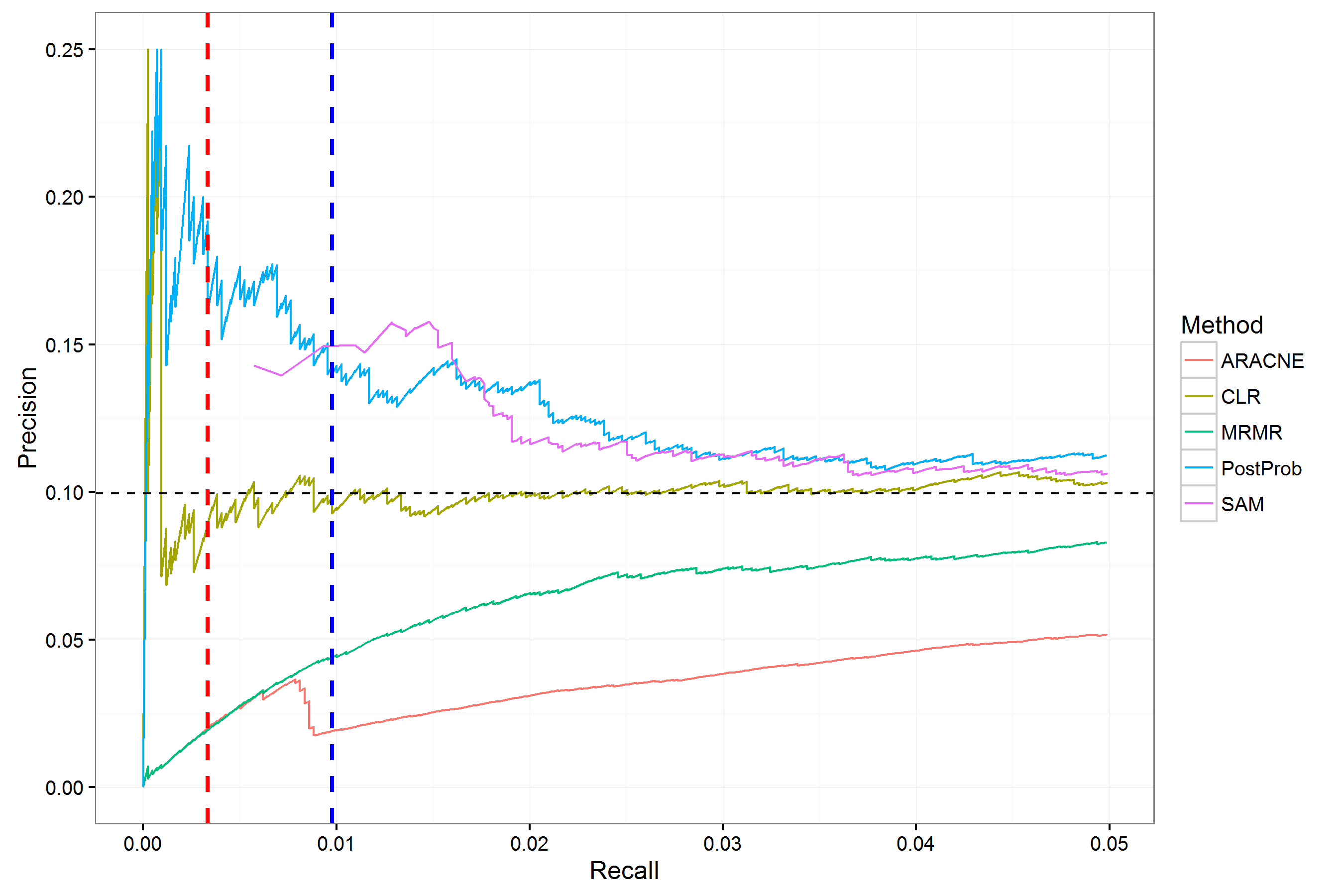
Figure 1: Precision-recall curves for cell line A375 using knockdown experiments for finding edges via posterior probability calculation evaluated against approximately 4,200 edges from TRANSFAC and JASPAR across 37 transcription factors. To the left of the red line are those edges with a posterior probability of at least 0.95, while the blue line shows the cutoff for edges with a posterior probability of 0.5. The horizontal dashed line shows the expected precision of 0.1 that would result from randomly ranking edges.

5 Discussion

We have demonstrated a straightforward approach to inferring gene regulatory network edges from knockdown data. This approach is simple to apply to large datasets and includes the ability to incorporate prior information when available. This approach is able to find confirmable regulatory relationships between genes from the L1000 data. We showed that our method performs comparably to or better than popular approaches for identifying important regulatory relationships as found in the TRANSFAC & JASPAR evaluation dataset.

One key benefit of this approach is that it can be applied to extremely large datasets, requiring only one read through the data to compile all sufficient statistics for computing the posterior probabilities. There is no need to retain all the data after reading it and no iterative methods, such as Expectation-Maximization or Markov Chain Monte Carlo, are used. Methods which model the entire network (Lèbre et al.,, 2010; Scutari,, 2010; McGeachie et al.,, 2014; Sanchez-Castillo et al.,, 2013) may yield more comprehensive network results but are also generally restricted to a smaller set of genes due to computational constraints. Our approach is complementary to these other approaches in potentially narrowing down the set of edges for further investigation.

We have applied the method to knockdown data in order to identify causal regulatory relationships. This method can also be applied to over-expression data or even steady-state data, although for steady-state data the resulting edges would lack directionality (Michailidis and d’Alché Buc,, 2013). This method could also be used to infer differential expression for a perturbation such as a drug treatment. This could be done using a 2-class model where the predictor variable indicates whether the expression measurements come from a perturbation experiment or a control experiment. An implementation of our method will be available as an r package, BayesKnockdown, including functions for both knockdown and perturbation data.

We considered using an edge reduction technique, such as that used by Pinna et al. (Pinna et al.,, 2010), but ultimately decided against it. Since we only used 37 genes as regulators due to our assessment data, the resulting networks did not tend to have multiple pathways from one gene to another. In cases where the resulting networks are much more rich in multi-gene pathways, using an edge reduction method may be appropriate.

Another possible use of this method is to use the resulting edge probabilities as an informed prior for another method utilizing a different type of data. This allows the integration of multiple data sources and may increase the usefulness of knockdown data that may expected to only provide a small amount of evidence within a larger experimental context.

References

- Basso et al., (2005) Basso, K., Margolin, A. A., Stolovitzky, G., Klein, U., Dalla-Favera, R., and Califano, A. (2005). Reverse engineering of regulatory networks in human B cells. Nature Genetics, 37:382–390.
- Chen et al., (2013) Chen, E. Y., Tan, C. M., Kou, Y., Duan, Q., Wang, Z., Meirelles, G. V., Clark, N. R., and Ma’ayan, A. (2013). Enrichr: interactive and collaborative HTML5 gene list enrichment analysis tool. BMC Bioinformatics, 14:128.
- Christley et al., (2004) Christley, S., Nie, Q., and Xie, X. (2004). Model uncertainty. PLoS One, pages 81–94.
- Christley et al., (2009) Christley, S., Nie, Q., and Xie, X. (2009). Incorporating existing network information into gene network inference. PLoS One, 4:article e6799.
- Dempster et al., (1977) Dempster, A. P., Laird, N. M., and Rubin, D. B. (1977). Maximum likelihood from incomplete data via the EM algorithm. Journal of the Royal Statistical Society. Series B (Methodological), pages 1–38.
- Ding and Peng, (2005) Ding, C. and Peng, H. (2005). Minimum redundancy feature selection from microarray gene expression data. Journal of Bioinformatics and Computational Biology, 3:185–205.
- Duan et al., (2014) Duan, Q., Flynn, C., Niepel, M., Hafner, M., Muhlich, J. L., Fernandez, N. F., Rouillard, A. D., Tan, C. M., Chen, E. Y., Golub, T. R., and others (2014). LINCS Canvas Browser: interactive web app to query, browse and interrogate LINCS L1000 gene expression signatures. Nucleic Acids Research, page article gku476.
- Dunbar, (2006) Dunbar, S. A. (2006). Applications of Luminex® xMAP™ technology for rapid, high-throughput multiplexed nucleic acid detection. Clinica Chimica Acta, 363:71–82.
- Faith et al., (2007) Faith, J. J., Hayete, B., Thaden, J. T., Mogno, I., Wierzbowski, J., Cottarel, G., Kasif, S., Collins, J. J., and Gardner, T. S. (2007). Large-scale mapping and validation of Escherichia coli transcriptional regulation from a compendium of expression profiles. PLoS Biol, 5:article e8.
- Fröhlich et al., (2007) Fröhlich, H., Fellmann, M., Sültmann, H., Poustka, A., and Bei\s sbarth, T. (2007). Large scale statistical inference of signaling pathways from rnai and microarray data. BMC Bioinformatics, 8:386.
- Friedman et al., (2000) Friedman, N., Linial, M., Nachman, I., and Pe’er, D. (2000). Using Bayesian networks to analyze expression data. Journal of Computational Biology, 7:601–620.
- Guelzim et al., (2002) Guelzim, N., Bottani, S., Bourgine, P., and Képès, F. (2002). Topological and causal structure of the yeast transcriptional regulatory network. Nature Genetics, 31:60–63.
- Gustafsson et al., (2009) Gustafsson, M., Hörnquist, M., Lundström, J., Björkegren, J., and Tegnér, J. (2009). Reverse engineering of gene networks with LASSO and nonlinear basis functions. Annals of the New York Academy of Sciences, 1158:265–275.
- Hoeting et al., (1999) Hoeting, J. A., Madigan, D., Raftery, A. E., and Volinsky, C. T. (1999). Bayesian model averaging: a tutorial. Statistical science, pages 382–401.
- Kim et al., (2004) Kim, S., Imoto, S., and Miyano, S. (2004). Dynamic Bayesian network and nonparametric regression for nonlinear modeling of gene networks from time series gene expression data. Biosystems, 75:57–65.
- Kim et al., (2003) Kim, S. Y., Imoto, S., Miyano, S., and others (2003). Inferring gene networks from time series microarray data using dynamic Bayesian networks. Briefings in Bioinformatics, 4:228–235.
- Klamt et al., (2010) Klamt, S., Flassig, R. J., and Sundmacher, K. (2010). TRANSWESD: inferring cellular networks with transitive reduction. Bioinformatics, 26:2160–2168.
- Lèbre et al., (2010) Lèbre, S., Becq, J., Devaux, F., Stumpf, M. P., and Lelandais, G. (2010). Statistical inference of the time-varying structure of gene-regulation networks. BMC Systems Biology, 4:article 130.
- Lo et al., (2012) Lo, K., Raftery, A. E., Dombek, K. M., Zhu, J., Schadt, E. E., Bumgarner, R. E., and Yeung, K. Y. (2012). Integrating external biological knowledge in the construction of regulatory networks from time-series expression data. BMC Systems Biology, 6:101.
- Marbach et al., (2010) Marbach, D., Prill, R. J., Schaffter, T., Mattiussi, C., Floreano, D., and Stolovitzky, G. (2010). Revealing strengths and weaknesses of methods for gene network inference. Proceedings of the National Academy of Sciences, 107:6286–6291.
- Marbach et al., (2009) Marbach, D., Schaffter, T., Mattiussi, C., and Floreano, D. (2009). Generating realistic in silico gene networks for performance assessment of reverse engineering methods. Journal of computational biology, 16:229–239.
- Margolin et al., (2006) Margolin, A. A., Nemenman, I., Basso, K., Wiggins, C., Stolovitzky, G., Favera, R. D., and Califano, A. (2006). ARACNE: an algorithm for the reconstruction of gene regulatory networks in a mammalian cellular context. BMC Bioinformatics, 7:article S7.
- McGeachie et al., (2014) McGeachie, M. J., Chang, H.-H., and Weiss, S. T. (2014). CGBayesNets: conditional Gaussian Bayesian Network learning and inference with mixed discrete and continuous data. PLoS Computational Biology, 10:article e1003676.
- Menéndez et al., (2010) Menéndez, P., Kourmpetis, Y. A., ter Braak, C. J., and van Eeuwijk, F. A. (2010). Gene regulatory networks from multifactorial perturbations using Graphical Lasso: application to the DREAM4 challenge. PloS One, 5:article e14147.
- Meyer et al., (2007) Meyer, P. E., Kontos, K., Lafitte, F., and Bontempi, G. (2007). Information-theoretic inference of large transcriptional regulatory networks. EURASIP Journal on Bioinformatics and Systems Biology, 2007:8–8.
- Meyer et al., (2008) Meyer, P. E., Lafitte, F., and Bontempi, G. (2008). minet: A R/Bioconductor package for inferring large transcriptional networks using mutual information. BMC Bioinformatics, 9:article 461.
- Michailidis and d’Alché Buc, (2013) Michailidis, G. and d’Alché Buc, F. (2013). Autoregressive models for gene regulatory network inference: Sparsity, stability and causality issues. Mathematical Biosciences, 246:326–334.
- Murphy et al., (1999) Murphy, K., Mian, S., and others (1999). Modelling gene expression data using dynamic Bayesian networks. Technical report, Technical report, Computer Science Division, University of California, Berkeley, CA.
- Pinna et al., (2010) Pinna, A., Soranzo, N., and De La Fuente, A. (2010). From knockouts to networks: establishing direct cause-effect relationships through graph analysis. PloS One, 5:article e12912.
- Raftery, (1999) Raftery, A. E. (1999). Bayes factors and BIC. Sociological Methods & Research, 27:411–417.
- Raftery et al., (1997) Raftery, A. E., Madigan, D., and Hoeting, J. A. (1997). Bayesian model averaging for linear regression models. Journal of the American Statistical Association, 92:179–191.
- Rogers and Girolami, (2005) Rogers, S. and Girolami, M. (2005). A Bayesian regression approach to the inference of regulatory networks from gene expression data. Bioinformatics, 21:3131–3137.
- Salleh et al., (2015) Salleh, F. H. M., Arif, S. M., Zainudin, S., and Raih, M. F. (2015). Reconstructing gene regulatory networks from knock-out data using Gaussian noise model and pearson correlation coefficient. Computational Biology and Chemistry.
- Sanchez-Castillo et al., (2013) Sanchez-Castillo, M., Tienda-Luna, I., Blanco, D., Carrion-Perez, M. C., and Huang, Y.-P. (2013). Bayesian sparse factor model for transcriptional regulatory networks inference. In Signal Processing Conference (EUSIPCO), 2013 Proceedings of the 21st European, pages 1–4. IEEE.
- Sandelin et al., (2004) Sandelin, A., Alkema, W., Engström, P., Wasserman, W. W., and Lenhard, B. (2004). JASPAR: an open-access database for eukaryotic transcription factor binding profiles. Nucleic Acids Research, 32:D91–D94.
- Scutari, (2010) Scutari, M. (2010). Learning Bayesian networks with the bnlearn R package. Journal of Statistical Software, 35:1–22.
- Shojaie et al., (2014) Shojaie, A., Jauhiainen, A., Kallitsis, M., and Michailidis, G. (2014). Inferring regulatory networks by combining perturbation screens and steady state gene expression profiles. PloS One, 9:article e82393.
- Tibshirani, (1996) Tibshirani, R. (1996). Regression shrinkage and selection via the lasso. Journal of the Royal Statistical Society. Series B (Methodological), pages 267–288.
- Tusher et al., (2001) Tusher, V. G., Tibshirani, R., and Chu, G. (2001). Significance analysis of microarrays applied to the ionizing radiation response. Proceedings of the National Academy of Sciences, 98:5116–5121.
- Verzelen, (2012) Verzelen, N. (2012). Minimax risks for sparse regressions: Ultra-high dimensional phenomenons. Electronic Journal of Statistics, 6:38–90.
- Wainwright, (2009) Wainwright, M. J. (2009). Sharp thresholds for high-dimensional and noisy sparsity recovery using-constrained quadratic programming (Lasso). IEEE Transactions on Information Theory, 55:2183–2202.
- Wingender et al., (2000) Wingender, E., Chen, X., Hehl, R., Karas, H., Liebich, I., Matys, V., Meinhardt, T., Prü\s s, M., Reuter, I., and Schacherer, F. (2000). TRANSFAC: an integrated system for gene expression regulation. Nucleic Acids Research, 28:316–319.
- Yeung et al., (2011) Yeung, K. Y., Dombek, K. M., Lo, K., Mittler, J. E., Zhu, J., Schadt, E. E., Bumgarner, R. E., and Raftery, A. E. (2011). Construction of regulatory networks using expression time-series data of a genotyped population. Proceedings of the National Academy of Sciences, 108:19436–19441.
- Yoo et al., (2002) Yoo, C., Thorsson, V., and Cooper, G. F. (2002). Discovery of causal relationships in a gene-regulation pathway from a mixture of experimental and observational DNA microarray data. In Pacific Symposium on Biocomputing, volume 7, pages 498–509.
- Young et al., (2014) Young, W. C., Raftery, A. E., and Yeung, K. Y. (2014). Fast Bayesian inference for gene regulatory networks using ScanBMA. BMC Systems Biology, 8:47.
- Zellner, (1986) Zellner, A. (1986). On assessing prior distributions and Bayesian regression analysis with g-prior distributions. Bayesian Inference and Decision Techniques: Essays in Honor of Bruno De Finetti, 6:233–243.
- Zou and Conzen, (2005) Zou, M. and Conzen, S. D. (2005). A new dynamic Bayesian network (DBN) approach for identifying gene regulatory networks from time course microarray data. Bioinformatics, 21:71–79.