Mobile Beamforming & Spatially Controlled Relay Communications

Abstract

We consider stochastic motion planning in single-source single-destination robotic relay networks, under a cooperative beamforming framework. Assuming that the communication medium constitutes a spatiotemporal stochastic field, we propose a $2$-stage stochastic programming formulation of the problem of specifying the positions of the relays, such that the expected reciprocal of their total beamforming power is maximized. Stochastic decision making is made on the basis of random causal CSI. Recognizing the intractability of the original problem, we propose a lower bound relaxation, resulting to a nontrivial optimization problem with respect to the relay locations, which is equivalent to a small set of simple, tractable subproblems. Our formulation results in spatial controllers with a predictive character; at each time slot, the new relay positions should be such that the expected power reciprocal at the next time slot is maximized. Quite interestingly, the optimal control policy to the relaxed problem is purely selective; under a certain sense, only the best relay should move.

1 Introduction

Cooperative beamforming constitutes a powerful method for information relaying in multi-hop networks. It is well known to greatly improve communication reliability by increasing directional channel gain, enabling low power, long distance transmissions with fewer hops, and with minimal interference [1, 2, 3]. In Amplify-and-Forward (AF) beamforming, which is considered here due to its simplicity [1], typically, the objective is to determine source power and/or relay beamforming weights so that certain optimality criteria are met, such as Quality-of-Service (QoS) at the destinations, or transmit power at the relays [1, 2, 3]. This optimization procedure critically depends on availability of Channel State Information (CSI) at the relays. In the literature, CSI is mostly assumed either known [2, 4, 5], or unknown with known statistics [1, 6, 7, 8, 9, 10], with the latter assumption better reflecting reality.

Recently, there has been works which exploit mobility of the relays assisting the communication, in order to further enhance performance in beamforming networks. In [11], mobility control has been combined with optimal transmit beamforming for transmit power minimization, while maintaining QoS in multiuser cooperative networks. Also, more recently [12], under a slightly different formulation, in the context of information theoretic secrecy, decentralized mobility control has been jointly combined with noise nulling and cooperative jamming for secrecy rate maximization in mobile jammer assisted cooperative communication networks with one source, one destination and multiple jammers. In the above works, the communication channels among the entities of the network (or the related second order statistics) have been assumed to be fixed during the whole motion of the relays. However, this assumption might be restrictive in scenarios where the channels change dynamically/stochastically through time and space.

In this paper, we present a novel treatment of the basic AF single-source single-destination relay beamforming problem, under the fundamental assumption that the channel, on the basis of which control decisions are determined, constitutes a spatiotemporal stochastic process. More specifically, we consider a time slotted, spatially controlled communication system, where, at each time slot, both communications and relay motion take place. Under this model, we propose a $2$-stage stochastic programming formulation of the problem of specifying the positions of the relays, such that the reciprocal of their total beamforming power is maximized on average, based on causal CSI. The proposed formulation results in relay spatial controllers with a predictive character; at each time slot, the decision on the new positions should be such that the expected power reciprocal, occurring at the next time slot, is maximized. Due to the intractability of the original problem, we propose a lower bound relaxation, which provably results to a nontrivial optimization problem with respect to the positions of the relays. Under a realistic “log-normal” wireless channel model [13], the relaxed problem is equivalent to solving a set of two dimensional, computationally tractable subproblems. Quite remarkably, the optimal control policy to the relaxed problem is purely selective; under a certain sense, only the best relay should move.

2 System Model

On a closed planar region ${\cal S}\subset\mathbb{R}^{2}$, we consider a wireless cooperative network consisting of one source, one destination and $R\in\mathbb{N}^{+}$ assistive relays. Each entity of the network is equipped with a single antenna, being able for both information reception and broadcasting/transmission. The source and destination are stationary and located at ${\bf p}_{S}\in{\cal S}$ and ${\bf p}_{D}\in{\cal S}$, respectively, whereas the relays are assumed to be mobile; each relay $i\in\mathbb{N}_{R}^{+}$ moves along a trajectory ${\bf p}_{i}\left(t\right)\in{\cal S}$, where, in general, $t\in\mathbb{R}_{+}$. We also define the supervector ${\bf p}\left(t\right)\triangleq\left[{\bf p}_{1}^{\boldsymbol{T}}\left(t\right)\,{\bf p}_{2}^{\boldsymbol{T}}\left(t\right)\,\ldots\,{\bf p}_{R}^{\boldsymbol{T}}\left(t\right)\right]^{\boldsymbol{T}}\in{\cal S}^{R}$. Additionally, we assume that the relays can cooperate with each other, either in terms of local message exchange, or by communicating with a local fusion center, through a dedicated channel.

Assuming that a direct link between the source and the destination does not exist, the role of the relays is determined to be assistive to the communication, in a classical two phase AF sense. Fix a $T>0$, and divide the time interval $\left[0,T\right]$ into $N_{T}$ time slots, with $t\in\mathbb{N}_{N_{T}}^{+}$ denoting the respective time slot. Let $s\left(t\right)\in\mathbb{C}$, with $\mathbb{E}\left\{\left|s\left(t\right)\right|^{2}\right\}\equiv 1$, denote the symbol to be transmitted at time slot $t$. Also, assuming a flat fading channel model, as well as channel reciprocity and quasistaticity in each time slot, let the sets $\left\{f_{i}\left({\bf p}_{i}\left(t\right),t\right)\in\mathbb{C}\right\}_{i\in\mathbb{N}_{R}^{+}}$ and $\left\{g_{i}\left({\bf p}_{i}\left(t\right),t\right)\in\mathbb{C}\right\}_{i\in\mathbb{N}_{R}^{+}}$ contain the random, spatiotemporally varying source-relay and relay-destination channel gains, respectively. Then, if $P_{0}>0$ denotes the transmission power, during AF phase $1$, relay $i$ receives the amplified symbol $\sqrt{P_{0}}s\left(t\right)$, modulated by $f_{i}\left({\bf p}_{i}\left(t\right),t\right)$, plus an additive, spatiotemporally white noise component $n_{i}\left(t\right)\in\mathbb{C}$, with $\mathbb{E}\left\{\left|n_{i}\left(t\right)\right|^{2}\right\}\equiv\sigma^{2}$, for all $i\in\mathbb{N}_{R}^{+}$. During AF phase $2$, all relays simultaneously retransmit the information received, each modulating their received signal by a weight $w_{i}\left(t\right)\in\mathbb{C},i\in\mathbb{N}_{R}^{+}$. The signal received at the destination can be expressed as the superposition of the weighted relay signals, plus another spatiotemporally white noise component $n_{D}\left(t\right)\in\mathbb{C}$, with $\mathbb{E}\left\{\left|n_{D}\left(t\right)\right|^{2}\right\}\equiv\sigma_{D}^{2}$.

In the following, whereas it is assumed that the stochastic processes $f_{i}\left({\bf p}_{i}\left(t\right),t\right)$ and $g_{j}\left({\bf p}_{t}\left(t\right),t\right)$ may be statistically dependent both spatially and temporally, for all $\left(i,j\right)\in\mathbb{N}_{R}^{+}\times\mathbb{N}_{R}^{+}$, it is also assumed that, as usual, the random processes $s\left(t\right)$, $\left[\left\{f_{i}\left({\bf p}_{i}\left(t\right),t\right),g_{i}\left({\bf p}_{i}\left(t\right),t\right)\right\}_{i\in\mathbb{N}_{R}^{+}}\right]$, $n_{i}\left(t\right)$ for all $i\in\mathbb{N}_{R}^{+}$, and $n_{D}\left(t\right)$ are mutually independent. Lastly, we will assume that, at each time slot $t,$ CSI $\left\{f_{i}\left({\bf p}_{i}\left(t\right),t\right)\right\}_{i\in\mathbb{N}_{R}^{+}}$ and $\left\{g_{i}\left({\bf p}_{i}\left(t\right),t\right)\right\}_{i\in\mathbb{N}_{R}^{+}}$ is known exactly to all relays. This may be achieved through pilot based estimation and will be considered a valid practical assumption.

3 Wireless Channel Modeling

At each time slot $t\in\mathbb{N}_{N_{T}}^{+}$, the $i$-th source-relay channel gain can be decomposed as [14]

$$f_{i}\left({\bf p}_{i}\left(t\right),t\right) \equiv\underbrace{f^{PL}\left({\bf p}_{i}\left(t\right)\right)}_{\text{path loss}}\underbrace{f_{i}^{SH}\left(t\right)}_{\text{shadowing}}\underbrace{f_{i}^{MF}\left(t\right)}_{\text{fading}}e^{\mathfrak{J}\frac{2\pi d_{iS}\left(t\right)}{\lambda}},$$ (1)

where $\mathfrak{J}\triangleq\sqrt{-1}$, $\lambda>0$ denotes the wavelength employed for the communication, and where: 1) $f^{PL}\left({\bf p}_{i}\left(t\right)\right)\triangleq\left\|{\bf p}_{i}\left(t\right)-{\bf p}_{S}\right\|_{2}^{-\ell/2}$ $\triangleq\left(d_{iS}\left(t\right)\right)^{-\ell/2}$, where $\ell>0$ denotes the path loss exponent. 2) $f_{i}^{SH}\left(t\right)\in\mathbb{R}$ denotes the shadowing part of the channel, whose square is a base-$10$ log-normal random variable with zero location. 3) $f_{i}^{MF}\left(t\right)\in\mathbb{C}$ represents multipath fading, which is assumed to be an unpredictable, spatiotemporally white [13], strictly stationary process with known statistics. In particular, its phase, $\phi_{f_{i}}\left(t\right)$, is assumed to be a white noise process uniformly distributed in $\left[-\pi,\pi\right]$, also independent of its magnitude.

Now, since the complex exponential in (1) is known, let us substitute $f_{i}\left({\bf p}_{i}\left(t\right),t\right)\leftarrow\exp\left(-\mathfrak{J}2\pi d_{iS}\left(t\right)/\lambda\right)$$f_{i}\left({\bf p}_{i}\left(t\right),t\right)$. Instead of working with the multiplicative model described by (1), it is much preferable to work in logarithmic scale. We may then define

$$F_{i}\left({\bf p}_{i}\left(t\right),t\right) \triangleq\alpha_{S}^{i}\left({\bf p}_{i}\left(t\right)\right)\ell+\sigma_{S}^{i}\left(t\right)+\xi_{S}^{i}\left(t\right),\;\forall i\in\mathbb{N}_{R}^{+}$$ (2)

and $\forall t\in\mathbb{N}_{N_{T}}^{+}$, where $\alpha_{S}^{i}\left({\bf p}_{i}\left(t\right)\right)\triangleq-10\log_{10}\left(d_{iS}\left(t\right)\right)$, $\sigma_{S}^{i}\left(t\right)\triangleq 10\log_{10}\left(f_{i}^{SH}\left(t\right)\right)^{2}$ and $\xi_{S}^{i}\left(t\right)\triangleq\overline{10\log_{10}\left|f_{i}^{MF}\left(t\right)\right|^{2}}$, with $\overline{\left(\cdot\right)}$ denoting the zero mean version of a random variable. Of course, we may stack all the $F_{i}\left({\bf p}_{i}\left(t\right),t\right)$’s defined in (2), resulting in the vector additive model

$$\boldsymbol{F}\left({\bf p}\left(t\right),t\right)\triangleq\boldsymbol{\alpha}_{S}\left({\bf p}\left(t\right)\right)\ell+\boldsymbol{\sigma}_{S}\left(t\right)+\boldsymbol{\xi}_{S}\left(t\right)\in\mathbb{R}^{R\times 1},$$ (3)

where $\boldsymbol{\alpha}_{S}\left(t\right)$, $\boldsymbol{\sigma}_{S}\left(t\right)$ and $\boldsymbol{\xi}_{S}\left(t\right)$ are defined accordingly. We can also define $\boldsymbol{G}\left({\bf p}\left(t\right),t\right)\triangleq\boldsymbol{\alpha}_{D}\left({\bf p}\left(t\right)\right)\ell+\boldsymbol{\sigma}_{D}\left(t\right)+\boldsymbol{\xi}_{D}\left(t\right)\in\mathbb{R}^{R\times 1},$ with each quantity in direct correspondence with (3).

The spatiotemporal dynamics of $\left\{f_{i}\left({\bf p}_{i}\left(t\right),t\right)\right\}_{i}$ and $\left\{g_{i}\left({\bf p}_{i}\left(t\right),t\right)\right\}_{i}$ are modeled through those of the shadowing components of $\left\{F_{i}\left({\bf p}_{i}\left(t\right),t\right)\right\}_{i}$ and $\left\{G_{i}\left({\bf p}_{i}\left(t\right),t\right)\right\}_{i}$. It is assumed that for any $N_{T}$, the process $\left[\left\{\boldsymbol{F}^{\boldsymbol{T}}\left({\bf p}\left(t\right),t\right)\,\boldsymbol{G}^{\boldsymbol{T}}\left({\bf p}\left(t\right),t\right)\right\}_{t\in\mathbb{N}_{N_{T}}^{+}}\right]^{\boldsymbol{T}}$ is jointly Gaussian with known means and known covariance matrix. More specifically [13], $\xi_{D\left(S\right)}^{i}\left(t\right)\overset{i.i.d.}{\sim}{\cal N}\left(0,\sigma_{\xi}^{2}\right)$, for all $t\in\mathbb{N}_{N_{T}}^{+}$ and $i\in\mathbb{N}_{R}^{+}$ [15]. Second, extending Gudmundson’s model [16] in a straightforward way, we propose defining the spatiotemporal correlations of the shadowing part of the channel as

$$\mathbb{E}\left\{\sigma_{S}^{i}\left(k\right)\sigma_{S}^{j}\left(l\right)\right\} \triangleq\eta^{2}e^{-\frac{\left\|{\bf p}_{i}\left(k\right)-{\bf p}_{j}\left(l\right)\right\|_{2}}{\beta}-\frac{\left|k-l\right|}{\gamma}},$$ (4)

and correspondingly for $\left\{\sigma_{D}^{i}\left(t\right)\right\}_{i\in\mathbb{N}_{R}^{+}}$, and additionally,

$$\mathbb{E}\left\{\sigma_{S}^{i}\left(k\right)\sigma_{D}^{j}\left(l\right)\right\} \triangleq\mathbb{E}\left\{\sigma_{S}^{i}\left(k\right)\sigma_{S}^{j}\left(l\right)\right\}e^{-\frac{\left\|{\bf p}_{S}-{\bf p}_{D}\right\|_{2}}{\delta}},$$ (5)

for all $\left(i,j\right)\in\mathbb{N}_{R}^{+}\times\mathbb{N}_{R}^{+}$ and all $\left(k,l\right)\in\mathbb{N}_{N_{T}}^{+}\times\mathbb{N}_{N_{T}}^{+}$. In the above, $\eta^{2}$ and $\beta>0$ are called the shadowing power and the correlation distance, respectively. In this fashion, we will call $\gamma>0$ and $\delta>0$ the correlation time and the BS (Base Station) correlation, respectively. For later reference, let us define the (cross)covariance matrices $\boldsymbol{\Sigma}_{SD}\left(t_{k},t_{l}\right)\triangleq\mathbb{E}\left\{\boldsymbol{\sigma}_{S}\left(t_{k}\right)\boldsymbol{\sigma}_{D}^{\boldsymbol{T}}\left(t_{l}\right)\right\}+\mathds{1}_{\left\{S\equiv D\right\}}\mathds{1}_{\left\{t_{k}\equiv t_{l}\right\}}\sigma_{\xi}^{2}{\bf I}_{R}$ $\in\mathbb{S}_{+\left(+\right)}^{R}$, as well as $\boldsymbol{\Sigma}\left(t_{k},t_{l}\right)\triangleq\left[\boldsymbol{\Sigma}_{SS}\left(t_{k},t_{l}\right)\,\boldsymbol{\Sigma}_{SD}\left(t_{k},t_{l}\right);\right.$ $\left.\boldsymbol{\Sigma}_{SD}\left(t_{k},t_{l}\right)\,\boldsymbol{\Sigma}_{DD}\left(t_{k},t_{l}\right)\right]\in\mathbb{S}_{+}^{2R}$.

4 Mobile Beamforming

At each time slot $t\in\mathbb{N}_{T}^{+}$ and assuming the same carrier for all communication tasks, we employ a basic joint communication/decision making TDMA-like protocol, as follows: 1) The source broadcasts a pilot signal to the relays, which then estimate the channels relative to the source. 2) The same procedure is carried out for the channels relative to the destination. 3) Then, based on the estimated CSI, beamforming is implemented. 4) Finally, based on the CSI received so far, the spatial controllers of the relays are determined, implementing accurate stochastic decision making.

In the following, let $\left\{\mathscr{C}\left({\cal T}_{t}\right)\right\}_{t\in\mathbb{N}_{N_{T}}^{+}}$ denote the set of channel gains observed by the relays, along the path of their point trajectories ${\cal T}_{i}\triangleq\left\{{\bf p}\left(t\right)\right\}_{t\in\mathbb{N}_{i}^{+}},i\in\mathbb{N}_{N_{T}}^{+}$, where ${\cal T}_{t}\equiv\left\{{\cal T}_{t-1},{\bf p}\left(t\right)\right\}$. Further, it is assumed that the motion of the relays obeys the differential equation $\dot{{\bf p}}\left(\tau\right)\equiv{\bf u}\left(\tau\right)$, for all $\tau\in\mathbb{R}_{+}$. Apparently, relay motion is in continuous time. However, assuming the relays move only after their controls have been determined and up to the start of the next time slot, we can write

$${\bf p}\left(t\right)\equiv{\bf p}\left(t-1\right)+\int_{\Delta\tau_{t-1}}{\bf u}_{t-1}\left(\tau\right)\text{d}\tau,\quad\forall t\in\mathbb{N}_{N_{T}}^{+},$$ (6)

with ${\bf p}\left(1\right)\equiv{\bf p}{}_{init}$, and where $\Delta\tau_{t}\in\mathbb{R}$ denotes the time interval that the relays are allowed to move in each time slot $t\in\mathbb{N}_{N_{T}}^{+}$. Of course, at each time slot $t$, $\Delta\tau_{t}$ must be sufficiently small such that the temporal correlations of the CSI at adjacent time slots are sufficiently strong. These correlations are controlled by the correlation time parameter $\delta$, which can be a function of the slot width. Therefore, the velocity of the relays must be of the order of $\left(\Delta\tau_{t}\right)^{-1}$. In this work, though, we assume that the relays are not resource constrained, in terms of their robotic operation. See Fig. 1 for a block representation of the proposed joint beamforming and relay motion control schema, where ${\cal I}_{t}$ contains the available CSI at time slot $t$ and $\left\{\cdot,\cdot\right\}$ denotes the concatenation operation.

4.1 $2$-Stage Stochastic Optimization of Beamforming Weights & Relay Positions

Suppose that, at time slot $t-1$, an oracle reveals $\mathscr{C}\left({\cal T}_{t}\right)$, which of course includes the channels corresponding to the new positions of the relays at the next time slot $t$. Then, given $\mathscr{C}\left({\cal T}_{t}\right)$, we are interested in determining $\boldsymbol{w}\left(t\right)\triangleq\left[w_{1}\left(t\right)\,w_{2}\left(t\right)\,\ldots\,w_{R}\left(t\right)\right]^{\boldsymbol{T}}$, as the solution of the power reciprocal maximization program

$$\begin{array}[]{rl}\underset{{\bf w}\left(t\right)}{\mathrm{maximize}}&\hskip 3.07pt\left(\mathbb{E}\left\{\left.P_{R}\right|\mathscr{C}\left({\cal T}_{t}\right)\right\}\right)^{-1}\\ \mathrm{subject\,to}&\dfrac{\mathbb{E}\left\{\left.P_{S}\right|\mathscr{C}\left({\cal T}_{t}\right)\right\}}{\mathbb{E}\left\{\left.P_{I+N}\right|\mathscr{C}\left({\cal T}_{t}\right)\right\}}\geq\zeta\end{array},$$ (7)

where $P_{R}$, $P_{S}$ and $P_{I+N}$ denote the instantaneous power at the relays, that of the signal component and that of the interference plus noise component at the destination, and where $\zeta>0$ is chosen such that (7) is feasible. Note that instead of minimizing the power at the relays, we are interested in maximizing its inverse, as this facilitates the formulation of our joint communication-control problem, as follows. Using the respective mutual independence assumptions, (7) can be written analytically and equivalently as [1]

$$\begin{array}[]{rl}\underset{{\bf w}\left(t\right)}{\mathrm{maximize}}&\hskip 7.3pt\left(\boldsymbol{w}^{\boldsymbol{H}}\left(t\right){\bf D}\left({\bf p}\left(t\right),t\right)\boldsymbol{w}\left(t\right)\right)^{-1}\\ \mathrm{subject\,to}&\dfrac{\boldsymbol{w}^{\boldsymbol{H}}\left(t\right){\bf R}\left({\bf p}\left(t\right),t\right)\boldsymbol{w}\left(t\right)}{\sigma_{D}^{2}+\boldsymbol{w}^{\boldsymbol{H}}\left(t\right){\bf Q}\left({\bf p}\left(t\right),t\right)\boldsymbol{w}\left(t\right)}\geq\zeta\end{array},$$ (8)

where, dropping the dependence on $\left({\bf p}\left(t\right),t\right)$ for brevity,

$${\bf D} \triangleq P_{0}\text{diag}\left(\left[\left|f_{1}\right|^{2}\,\left|f_{2}\right|^{2}\,\ldots\,\left|f_{R}\right|^{2}\right]^{\boldsymbol{T}}\right)+\sigma^{2}{\bf I}_{R}\in\mathbb{S}_{++}^{R},$$ (9)

$${\bf R} \triangleq P_{0}{\bf h}{\bf h}^{\boldsymbol{H}}\in\mathbb{S}_{+}^{R},\text{ with }{\bf h}\triangleq\left[f_{1}g_{1}\,f_{2}g_{2}\,\ldots\,f_{R}g_{R}\right]^{\boldsymbol{T}}\text{ and}$$ (10)

$${\bf Q} \triangleq\sigma^{2}\text{diag}\left(\left[\left|g_{1}\right|^{2}\,\left|g_{2}\right|^{2}\,\ldots\,\left|g_{R}\right|^{2}\right]^{\boldsymbol{T}}\right)\in\mathbb{S}_{++}^{R}.$$ (11)

Obviously, if the oracle could reveal $\mathscr{C}\left(\left\{{\cal T}_{t-1},{\bf p}\left(t\right)\right\}\right)$ at $t-1$, we could further optimize the optimal value of (8) with respect to ${\bf p}\left(t\right)$, representing the new position of the relays. In the absence of the oracle, though, this is impossible, since given $\mathscr{C}\left(\left\{{\cal T}_{t-1}\right\}\right)$, the channels at any position of the relays are nontrivial random variables. However, given $\mathscr{C}\left(\left\{{\cal T}_{t-1}\right\}\right)$, it is reasonable to search for the best decision on the positions of the relays at time slot $t$ (as a functional of $\mathscr{C}\left(\left\{{\cal T}_{t-1}\right\}\right)$), such that the optimal value of (8) is maximized, on average. This results in the $2$-stage stochastic program [17]

$$\begin{array}[]{rl}\underset{{\bf p}\left(t\right)}{\mathrm{maximize}}&\mathbb{E}\left\{V\left({\bf p}\left(t\right),t\right)\right\}\\ \mathrm{subject\,to}&{\cal C}\left({\bf p}\left(t-1\right)\right)\ni{\bf p}\left(t\right)\equiv\mathbb{E}\left\{\left.{\bf p}\left(t\right)\right|\mathscr{C}\left({\cal T}_{t-1}\right)\right\}\end{array},$$ (12)

where

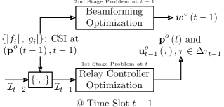
Fig. 1: 2-Stage optimization of beamforming weights and spatial relay controllers. $\boldsymbol{w}^{o}\left(t-1\right)$, ${\bf u}_{t-1}^{o}\left(\tau\right)$ and ${\bf p}^{o}\left(t\right)$ denote the optimal beamforming weights and relay controllers at time slot $t-1$ and the optimal relay positions at time slot $t$, respectively. Also, ${\cal I}_{0}\equiv\left\{\varnothing\right\}$.

the random variable $V\left({\bf p}\left(t\right),t\right)$ (a functional of $\mathscr{C}\left({\cal T}_{t}\right)$) denotes the optimal value of (8), and ${\cal C}\left({\bf p}\left(t-1\right)\right)$ denotes a convex set, representing a spatially feasible neighborhood around ${\bf p}\left(t-1\right)$. Problems (12) and (8) are referred to as the first-stage problem and the second-stage problem, respectively [17] (also see Fig. 1). In general, the existence of elegant solutions for $2$-stage problems is extremely rare. Fortunately, however, in our case, the second-stage problem admits a (semi)closed form solution, expressed as [1]

$$V=\dfrac{\lambda_{max}\left({\bf D}^{-1/2}\left({\bf R}-\zeta{\bf Q}\right){\bf D}^{-1/2}\right)}{\zeta\sigma_{D}^{2}}\triangleq\dfrac{\lambda_{max}\left({\bf B}\right)}{\zeta\sigma_{D}^{2}}.$$ (13)

The resulting equivalent form for problem (12) is still difficult to solve because of two reasons; its variational character and, second, the fact that the expectation in the objective cannot be computed in any reasonable and tractable way. By an application of a generalized form of the fundamental lemma of stochastic control [18, 19], the first stage problem (12) can be equivalently replaced by the much simpler problem

$$\underset{{\bf p}\left(t\right)\in{\cal C}\left({\bf p}\left(t-1\right)\right)}{\mathrm{maximize}}\mathbb{E}\left\{\left.\lambda_{max}\left({\bf B}\left({\bf p}\left(t\right),t\right)\right)\right|\mathscr{C}\left({\cal T}_{t-1}\right)\right\},$$ (14)

perfectly solving the first issue mentioned above. Regarding now the second issue arising as a result of the (conditional) expectation appearing in (14), due to the convexity of the maximum eigenvalue operator in ${\bf B}$, we can use Jensen’s Inequality in order to lower bound the objective of (14) by the quantity $\lambda_{max}\left(\mathbb{E}\left\{\left.{\bf B}\left({\bf p}\left(t\right),t\right)\right|\mathscr{C}\left({\cal T}_{t-1}\right)\right\}\right)$, resulting in the lower bound relaxation

$$\underset{{\bf p}\left(t\right)\in{\cal C}\left({\bf p}\left(t-1\right)\right)}{\mathrm{maximize}}\lambda_{max}\left(\mathbb{E}\left\{\left.{\bf B}\left({\bf p}\left(t\right),t\right)\right|\mathscr{C}\left({\cal T}_{t-1}\right)\right\}\right).$$ (15)

Apparently, the challenge now is to properly express the conditional expectation involved as an explicit functional of ${\bf p}\left(t\right)$. Interestingly, it can be shown that the random matrix $\boldsymbol{E}\left({\bf p}\left(t\right)\right)\triangleq\mathbb{E}\left\{\left.{\bf B}\left({\bf p}\left(t\right),t\right)\right|\mathscr{C}\left({\cal T}_{t-1}\right)\right\}$ (where we emphasize the dependence on ${\bf p}\left(t\right)$) is diagonal, with elements

$$\boldsymbol{E}_{i} \triangleq\mathbb{E}\left\{\left.\dfrac{P_{0}\left|f_{i}\right|^{2}\left|g_{i}\right|^{2}-\zeta\sigma^{2}\left|g_{i}\right|^{2}}{P_{0}\left|f_{i}\right|^{2}+\sigma^{2}}\right|\mathscr{C}\left({\cal T}_{t-1}\right)\right\},\;i\in\mathbb{N}_{R}^{+}.$$ (16)

In order to evaluate the conditional expectations in each diagonal element of $\boldsymbol{E}$, hereafter, we will assume that $1/\left(P_{0}\left|f_{i}\right|^{2}+\sigma^{2}\right)$ $\approx 1/\left(P_{0}\left|f_{i}\right|^{2}\right)$, for all $i\in\mathbb{N}_{R}^{+}$, corresponding to a high-SNR scenario at the relays. This approximation will be valid if either the noise power at the relays is small, or the broadcasting power of the source is relatively large. This situation is reasonable in beamforming networks, since the most suitable network nodes in terms of information relaying may be selected through a relay selection procedure. Then, (16) becomes

$$\boldsymbol{E}_{i}=\mathbb{E}\left\{\left.\left|g_{i}\right|^{2}\right|\mathscr{C}\left({\cal T}_{t-1}\right)\right\}-\dfrac{\zeta\sigma^{2}}{P_{0}}\mathbb{E}\left\{\left.\left|g_{i}\right|^{2}\left|f_{i}\right|^{-2}\right|\mathscr{C}\left({\cal T}_{t-1}\right)\right\},$$ (17)

for all $i\in\mathbb{N}_{R}^{+}$. In fact, each $\boldsymbol{E}_{i}$ may be computed in closed form, as the following result suggests.

Theorem 1.

(Conditional Correlations) Under the wireless channel modeling assumptions of Section 3, it is true that

$$\mathbb{E}\left\{\left.\left|g_{i}\right|^{2}\right|\mathscr{C}\left({\cal T}_{t-1}\right)\right\}\equiv 10^{\rho/10}\exp\left(\vphantom{\dfrac{\log^{2}\left(10\right)}{200}\sigma_{\left.t\right|t-1}^{2,G_{i}}\left({\bf p}_{i}\left(t\right)\right)}\dfrac{\log\left(10\right)}{10}\mu_{\left.t\right|t-1}^{G_{i}}\left({\bf p}_{i}\left(t\right)\right)\right.\\ \left.+\dfrac{\log^{2}\left(10\right)}{200}\sigma_{\left.t\right|t-1}^{2,G_{i}}\left({\bf p}_{i}\left(t\right)\right)\right),\quad\text{and}\\ \mathbb{E}\left\{\left.\left|g_{i}\right|^{2}\left|f_{i}\right|^{-2}\right|\mathscr{C}\left({\cal T}_{t-1}\right)\right\}\equiv\exp\left(\vphantom{\dfrac{\log^{2}\left(10\right)}{200}\begin{bmatrix}1\\ -1\end{bmatrix}^{\boldsymbol{T}}\boldsymbol{\Sigma}_{\left.t\right|t-1}^{G_{i},F_{i}}\left({\bf p}_{i}\left(t\right)\right)\begin{bmatrix}1\\ -1\end{bmatrix}}\dfrac{\log\left(10\right)}{10}\left(\mu_{\left.t\right|t-1}^{G_{i}}\left({\bf p}_{i}\left(t\right)\right)\right.\right.\\ \left.\left.-\mu_{\left.t\right|t-1}^{F_{i}}\left({\bf p}_{i}\left(t\right)\right)\right)+\dfrac{\log^{2}\left(10\right)}{200}\begin{bmatrix}1\\ -1\end{bmatrix}^{\boldsymbol{T}}\boldsymbol{\Sigma}_{\left.t\right|t-1}^{G_{i},F_{i}}\left({\bf p}_{i}\left(t\right)\right)\begin{bmatrix}1\\ -1\end{bmatrix}\right).$$ (18)

In (18), we define $\rho\triangleq 10\mathbb{E}\left\{\log_{10}\left|f_{i}^{MF}\left(t\right)\right|^{2}\right\}$, and

$$\mu_{\left.t\right|t-1}^{G_{i}}\left(\cdot\right) \triangleq\alpha_{D}\left(\cdot\right)\ell+\boldsymbol{c}_{1:t-1}^{G_{i}}\left(\cdot\right)\boldsymbol{\Sigma}_{1:t-1}^{-1}\left(\boldsymbol{m}_{1:t-1}-\boldsymbol{\mu}_{1:t-1}\right),$$ (19)

$$\sigma_{\left.t\right|t-1}^{2,G_{i}}\left(\cdot\right) \triangleq\sigma_{\xi}^{2}+\eta^{2}-\boldsymbol{c}_{1:t-1}^{G_{i}}\left(\cdot\right)\boldsymbol{\Sigma}_{1:t-1}^{-1}\left[\boldsymbol{c}_{1:t-1}^{G_{i}}\left(\cdot\right)\right]^{\boldsymbol{T}},\text{ with}$$ (20)

$$\boldsymbol{c}_{1:t-1}^{G_{i}}\left(\cdot\right) \triangleq\left[\left\{\boldsymbol{c}_{k}^{G_{i}}\right\}_{k\in\mathbb{N}_{t-1}^{+}}\right],$$ (21)

and

$$\boldsymbol{m}_{1:t-1} \triangleq\left[\left\{\boldsymbol{F}^{\boldsymbol{T}}\left({\bf p}\left(j\right),j\right)\,\boldsymbol{G}^{\boldsymbol{T}}\left({\bf p}\left(j\right),j\right)\right\}_{j\in\mathbb{N}_{t-1}^{+}}\right]^{\boldsymbol{T}},$$ (22)

$$\boldsymbol{\mu}_{1:t-1} \triangleq\left[\left\{\boldsymbol{\alpha}_{S}\left(j\right)\,\boldsymbol{\alpha}_{D}\left(j\right)\right\}_{j\in\mathbb{N}_{t-1}^{+}}\right]^{\boldsymbol{T}}\ell,$$ (23)

$$\boldsymbol{\Sigma}_{1:t-1} \triangleq\begin{bmatrix}\boldsymbol{\Sigma}\left(1,1\right)&\cdots&\boldsymbol{\Sigma}\left(1,t-1\right)\\ \vdots&\ddots&\vdots\\ \boldsymbol{\Sigma}\left(t-1,1\right)&\cdots&\boldsymbol{\Sigma}\left(t-1,t-1\right)\end{bmatrix},$$ (24)

$$\boldsymbol{c}_{k}^{G_{i}} \triangleq\left[\left\{\mathbb{E}\left\{\sigma_{D}^{i}\left(t\right)\sigma_{S}^{j}\left(k\right)\right\}\right\}_{j}\,\left\{\mathbb{E}\left\{\sigma_{D}^{i}\left(t\right)\sigma_{D}^{j}\left(k\right)\right\}\right\}_{j}\right],$$ (25)

where $\boldsymbol{c}_{1:t-1}^{G_{i}}\left(\cdot\right)\in\mathbb{R}^{1\times\left(t-1\right)2R}$,$\boldsymbol{m}_{1:t-1}$ and $\boldsymbol{\mu}_{1:t-1}$ are in $\mathbb{R}^{\left(t-1\right)2R\times 1}$ and $\boldsymbol{\Sigma}_{1:t-1}$ is in $\mathbb{S}_{++}^{\left(t-1\right)2R}$, for all $t\in\mathbb{N}_{N_{T}}^{+}$. In (18), we have

$$\boldsymbol{\Sigma}_{\left.t\right|t-1}^{G_{i},F_{i}}\left(\cdot\right) \equiv\begin{bmatrix}\eta^{2}+\sigma_{\xi}^{2}&\eta^{2}e^{-\frac{\left\|{\bf p}_{S}-{\bf p}_{D}\right\|_{2}}{\delta}}\\ \eta^{2}e^{-\frac{\left\|{\bf p}_{S}-{\bf p}_{D}\right\|_{2}}{\delta}}&\eta^{2}+\sigma_{\xi}^{2}\end{bmatrix}$$

$$-\begin{bmatrix}\boldsymbol{c}_{1:t-1}^{G_{i}}\left(\cdot\right)\\ \boldsymbol{c}_{1:t-1}^{F_{i}}\left(\cdot\right)\end{bmatrix}\boldsymbol{\Sigma}_{1:t-1}^{-1}\begin{bmatrix}\boldsymbol{c}_{1:t-1}^{G_{i}}\left(\cdot\right)\\ \boldsymbol{c}_{1:t-1}^{F_{i}}\left(\cdot\right)\end{bmatrix}^{\boldsymbol{T}}\in\mathbb{R}^{2\times 2},$$ (26)

and the quantities $\mu_{\left.t\right|t-1}^{F_{i}}\left(\cdot\right)$ and $\boldsymbol{c}_{1:t-1}^{F_{i}}\left(\cdot\right)$ are defined accordingly, swapping “$D$” and “$S$” where applicable.

Theorem 1 implies that (17) can be explicitly expressed in terms of the available CSI and the related statistics. This is possible due to the Gaussianity of the log-squared magnitude of the observed channels. The proof involves the evaluation of the related conditional moment generating functions and it is omitted due to lack of space.

From (18), one can observe that (17) is a well defined functional of ${\bf p}_{i}\left(t\right)$, that is, $\boldsymbol{E}_{i}\equiv\boldsymbol{E}_{i}\left({\bf p}_{i}\left(t\right)\right)$, for all $i\in\mathbb{N}_{R}^{+}$. Additionally, as it was expected, each $\boldsymbol{E}_{i}$ is independent of all ${\bf p}_{j}\left(t\right),j\neq i$. Under these circumstances, the program under consideration, described by (15), can be expressed as the maximization of $\boldsymbol{E}_{i}\left({\bf p}_{i}\left(t\right)\right)$ jointly over ${\bf p}\left(t\right)\in{\cal C}\left({\bf p}\left(t-1\right)\right)$ and $i\in\mathbb{N}_{R}^{+}$, which is equivalent to

$$\underset{i\in\mathbb{N}_{R}^{+}}{\mathrm{max}}\left[\underset{{\bf p}_{i}\left(t\right)\in{\cal C}\left({\bf p}_{i}\left(t-1\right)\right)}{\mathrm{max}}\boldsymbol{E}_{i}\left({\bf p}_{i}\left(t\right)\right)\right].$$ (27)

In particular, each of the $R$ two dimensional problems involved can be performed locally at each relay, provided the availability of common global information (channel magnitudes and relay positions).

Quite remarkably, the discussion above reveals that the optimal control policy is of a purely selective form: At each $t\in\mathbb{N}_{N_{T}}^{+}$ and provided that the inner problem of (27) can be solved exactly, only the $i^{o}$-th relay should move, where $i^{o}$ is the respective solution of the outer maximization of (27); in fact, either any of the rest of the relays moves or not is irrelevant.

4.2 Determination of Relay Motion Controllers

What remains now is to determine the controllers of the $i^{o}$-th relay, selected to carry out the decision that optimizes the relaxed cost of (15). Suppose that ${\bf p}^{o}\left(t\right)\in\underset{{\bf p}_{i}\left(t\right),i}{\mathrm{arg\,max}}\boldsymbol{E}_{i}\left({\bf p}_{i}\left(t\right)\right)$ has been determined, for instance, numerically. Then, it suffices to fix a path in ${\cal S}$, such that the points ${\bf p}^{o}\left(t\right)$ and ${\bf p}_{i^{o}}\left(t-1\right)$ are connected in at most time $\Delta\tau_{t}$. By far the easiest choice for such a path is the straight line connecting ${\bf p}^{o}\left(t\right)\triangleq\left[x_{t}^{o}\,y_{t}^{o}\right]^{\boldsymbol{T}}$ and ${\bf p}_{i^{o}}\left(t-1\right)\triangleq\left[x_{t-1}^{i^{o}}\,y_{t-1}^{i^{o}}\right]^{\boldsymbol{T}}$. Therefore, we can choose the optimal relay motion controller as

$${\bf u}_{t-1}^{o}\left(\tau\right)\triangleq\dfrac{1}{\Delta\tau_{t-1}}\begin{bmatrix}y_{t}^{o}-y_{t-1}^{i^{o}}\\ x_{t}^{o}-x_{t-1}^{i^{o}}\end{bmatrix},\quad\tau\in\Delta\tau_{t-1},$$ (28)

completing the presentation of the proposed solution to the mobile beamforming problem under consideration.

5 Conclusion

We have considered the problem of stochastic relay spatial control for beamforming optimization in single-source single-destination robotic relay networks. Under a realistic spatiotemporal stochastic model for the communication medium, we proposed a $2$-stage stochastic programming formulation for specifying relay spatial controllers, such that the future expected reciprocal of their total beamforming power is maximized, based only on causal CSI at the relays. Due to the intractability of the original problem, we have proposed a lower bound relaxation, which is equivalent to a set of tractable two dimensional subproblems, solved at each relay independently. Interestingly, the aforementioned formulation results to a relay selection plus control scheme; at each time slot, only one relay should move - the one resulting to the highest expected beamforming improvement. This work essentially serves as a basis for several extended formulations of the mobile beamforming problem and more generally of related problems in spatially controlled communication systems; these constitute the subject of current research.

References

- [1] V. Havary-Nassab, S. ShahbazPanahi, A. Grami, and Zhi-Quan Luo, “Distributed beamforming for relay networks based on second-order statistics of the channel state information,” Signal Processing, IEEE Transactions on, vol. 56, no. 9, pp. 4306–4316, Sept 2008.
- [2] Y. Jing and H. Jafarkhani, “Network beamforming using relays with perfect channel information,” Information Theory, IEEE Transactions on, vol. 55, no. 6, pp. 2499–2517, June 2009.
- [3] G. Zheng, Kai-Kit Wong, A. Paulraj, and B. Ottersten, “Collaborative-relay beamforming with perfect csi: Optimum and distributed implementation,” Signal Processing Letters, IEEE, vol. 16, no. 4, pp. 257–260, April 2009.
- [4] L. Dong, A.P. Petropulu, and H.V. Poor, “Weighted cross-layer cooperative beamforming for wireless networks,” Signal Processing, IEEE Transactions on, vol. 57, no. 8, pp. 3240–3252, Aug 2009.
- [5] V. Havary-Nassab, S. ShahbazPanahi, and A. Grami, “Optimal distributed beamforming for two-way relay networks,” Signal Processing, IEEE Transactions on, vol. 58, no. 3, pp. 1238–1250, March 2010.
- [6] E. Koyuncu, Y. Jing, and H. Jafarkhani, “Distributed beamforming in wireless relay networks with quantized feedback,” Selected Areas in Communications, IEEE Journal on, vol. 26, no. 8, pp. 1429–1439, October 2008.
- [7] S. Fazeli-Dehkordy, S. ShahbazPanahi, and S. Gazor, “Multiple peer-to-peer communications using a network of relays,” Signal Processing, IEEE Transactions on, vol. 57, no. 8, pp. 3053–3062, Aug 2009.
- [8] J. Li, A.P. Petropulu, and H.V. Poor, “Cooperative transmission for relay networks based on second-order statistics of channel state information,” Signal Processing, IEEE Transactions on, vol. 59, no. 3, pp. 1280–1291, March 2011.
- [9] Y. Liu and A.P. Petropulu, “On the sumrate of amplify-and-forward relay networks with multiple source-destination pairs,” Wireless Communications, IEEE Transactions on, vol. 10, no. 11, pp. 3732–3742, November 2011.
- [10] Y. Liu and A.P. Petropulu, “Relay selection and scaling law in destination assisted physical layer secrecy systems,” in Statistical Signal Processing Workshop (SSP), 2012 IEEE, Aug 2012, pp. 381–384.
- [11] N. Chatzipanagiotis, Yupeng Liu, A. Petropulu, and M.M. Zavlanos, “Controlling groups of mobile beamformers,” in Decision and Control (CDC), 2012 IEEE 51st Annual Conference on, Dec 2012, pp. 1984–1989.
- [12] D. S. Kalogerias, N. Chatzipanagiotis, M. M. Zavlanos, and A. P. Petropulu, “Mobile jammers for secrecy rate maximization in cooperative networks,” in Acoustics, Speech and Signal Processing (ICASSP), 2013 IEEE International Conference on, May 2013, pp. 2901–2905.
- [13] M. Malmirchegini and Y. Mostofi, “On the spatial predictability of communication channels,” Wireless Communications, IEEE Transactions on, vol. 11, no. 3, pp. 964–978, March 2012.
- [14] A. Goldsmith, Wireless communications, Cambridge university press, 2005.
- [15] S. L. Cotton and W. G. Scanlon, “Higher order statistics for lognormal small-scale fading in mobile radio channels,” Antennas and Wireless Propagation Letters, IEEE, vol. 6, pp. 540–543, 2007.
- [16] M. Gudmundson, “Correlation model for shadow fading in mobile radio systems,” Electronics Letters, vol. 27, no. 23, pp. 2145–2146, Nov 1991.
- [17] A. Shapiro, D. Dentcheva, and A. Ruszczynski, Lectures on Stochastic Programming: Modeling and Theory (MPS-SIAM Series on Optimization), SIAM-Society for Industrial and Applied Mathematics, 2009.
- [18] J. L. Speyer and W. H. Chung, Stochastic processes, estimation, and control, vol. 17, Siam, 2008.
- [19] K. J. Astrom, Introduction to stochastic control theory, vol. 70, New York: Academic Press, 1970.