Reduced Wiener Chaos representation of random fields via basis adaptation and projection

Abstract

A new characterization of random fields appearing in physical models is presented that is based on their well-known Homogeneous Chaos expansions. We take advantage of the adaptation capabilities of these expansions where the core idea is to rotate the basis of the underlying Gaussian Hilbert space, in order to achieve reduced functional representations that concentrate the induced probability measure in a lower dimensional subspace. For a smooth family of rotations along the domain of interest, the uncorrelated Gaussian inputs are transformed into a Gaussian process, thus introducing a mesoscale that captures intermediate characteristics of the quantity of interest.

1 Introduction

Modeling, characterizing and propagating uncertainties in complex physical systems have been extensively explored in recent years as they straddle engineering and the physical, computational, and mathematical sciences. The computational burden associated with a probabilistic representation of these uncertainties is a persistent related challenge. One class of approaches to this challenge has been to seek proper functional representations of the quantities of interest (QoI) under investigation that will be consistent with the observed reality as well as with the mathematical formulation of the underlying physical system, which for instance, is characterized within the context of partial differential equations with stochastic parameters. Additionally, these representations are equipped to serve as accurate propagators useful for prediction or statistical inference purposes. Among the criteria that make such a functional representation a successful candidate, are often the ability to provide a parametric interpretation of the uncertainties involved in a subscale level of the governing physics, as well as its quality as an approximation of what is assumed to be the reality and its discrepancy from it, in terms of several modes of convergence such as distributional, almost sure or functional ($L^{2}$).

The Homogeneous (Wiener) Chaos [35] representation of random processes has provided a convenient way to characterize solutions of systems of equations that describe physical phenomena as was demonstrated in [15] and further applied to a wide range of engineering problems [11, 25, 10, 12, 14]. Generalization of these representations beyond the Gaussian white noise [36, 30] provided the foundation for a multi-purpose tool for uncertainty characterization and propagation [21, 27, 37], statistical updating [29, 23, 24] and design [17, 33] or as a generic mathematical model in order to characterize uncertainties using maximum likelihood techniques [6, 16], Bayesian inference [13, 2] or maximum entropy [5]. Despite its wide applicability which has resulted in significant gains, including but not limited to computational efficiencies, its use can still easily become prohibitive with the increase of the dimensionality of the stochastic input. Several attempts using sparse representations [8, 7] have only partially managed to sidestep the issue which still remains a major drawback. Recently, a new method for adapted Chaos expansions in Homogeneous Chaos spaces has shown some promising potential as a generic dimensionality reduction technique [32]. The core idea is based on rotating the independent Gaussian inputs through a suitable isometry to form a new basis such that the new expansion expressed in terms of that basis concentrates its probability measure in a lower dimensional subspace, consequently, the basis terms of the Homogeneous Chaos spaces that lie outside that subspace can be filtered out via a projection procedure. Several special cases along with intrusive and non-intrusive computational algorithms were suggested which result in significant model reduction while maintaining high fidelity in the probabilistic characterization of the scalar QoIs.

It is the main objective of the present paper to extend further the basis adaptation technique from simple scalar quantities of interest to random fields or vector valued quantities that admit a polynomial chaos expansion. Such random fields emerge, for instance, as solutions of partial differential equations with random parameters and can be found to have different degree of dependence on the stochastic inputs at different spatio-temporal locations, therefore their adapted representations and the corresponsing adapted basis should be expected to exhibit such a spatio-temporal dependence. We provide a general framework where a family of isometries are indexed by the same topological space used for indexing the random field of interest. Several important properties are proved for the new adapted expansion, namely the new stochastic input is no longer a vector of standard normal variables but a Gaussian random field that admits a Karhunen-Loeve [20, 22] expansion with respect to those variables. This new quantity essentially merges uncertainties into a new basis that varies at different locations, thus introducing a new way of upscaling uncertainties with localized information about the quantity of interest. In addition, new explicit formulas are derived that allow the transformation of an existing chaos expansion to a new expansion with respect to any chosen basis. One major benefit of this capability is that, once a chaos expansion is available, any suitable adaptation can be achieved without further relying on intrusive and non-intrusive methods that would require additional (repeated) evaluations of the mathematical model, thus delivering us from further computational costs.

This paper is organized as follows: First we introduce the basis adaptation framework for Homogeneous Chaos expansions and the reduction procedure via projection on subspaces of the Hilbert space of square integrable random fields. Next we demonstrate how the framework applies when stochasticity is also present in the coefficients of the chaos expansion and finally we provide the theoretical foundations of an infinite dimensional perspective of our approach which shows that our derivations remain consistent and are nothing more but a special case of Hilbert spaces of arbitrary dimension. Finally, our results are illustrated with two numerical examples: That of an elliptic PDE with random diffusion parameter, which explores various ways of obtaining reduced order expansions that adapt well on the random field of interest and an explicit chaos expansion where its first order coefficients consist of a geometric series which allows the comparison of infinite dimensional adaptations and their truncated versions.

2 Basis adaptation in Homogeneous Chaos expansions of random fields

2.1 The Homogeneous (Wiener) Chaos

We consider a probability space $\left(\Omega,\mathcal{F},\mathbb{P}\right)$ and $\mathcal{G}$ a $d$-dimensional Gaussian Hilbert space, that is a closed vector space spanned by a set of $d$ independent standard (zero-mean and unit-variance) Gaussian random variables $\{\xi_{i}\}_{i=1}^{d}$, equipped with the inner product $\langle\cdot,\cdot\rangle_{\mathcal{G}}$ defined as $\langle\xi,\zeta\rangle_{\mathcal{G}}=\mathbb{E}[\xi\zeta]$ for $\xi,\zeta\in H$, where $\mathbb{E}[\cdot]$ denotes the mathematical expectation with respect to the probability measure $\mathbb{P}$. For simplicity, throughtout this section we will drop the index _G and simply write $\langle\cdot,\cdot\rangle$ whenever there is no confusion. Let now $\mathcal{F}(\mathcal{G})$ be the $\sigma$-algebra generated by the elements of $\mathcal{G}$, then since all Gaussian variables have finite second moments, it follows that $\mathcal{G}$ is a closed subspace of $L^{2}(\Omega,\mathcal{F}(\mathcal{G}),\mathbb{P})$. We also define $\mathcal{G}^{\diamond n}$, for $n\in\mathbb{N}\cup\{-1,0\}$ to be the space of all polynomials of exact order $n$, with the convention $\mathcal{G}^{\diamond-1}:=\{0\}$. Then clearly $\mathcal{G}^{\diamond 0}$ is the space of constants and $\mathcal{G}^{\diamond 1}=\mathcal{G}$ and in fact from the Cameron-Martin theorem [3, 19] we have that $L^{2}(\Omega,\mathcal{F}(\mathcal{G}),\mathbb{P})=\bigoplus_{n=0}^{\infty}\mathcal{G}^{\diamond n}$ which has an orhogonal basis that consists of the multidimensional Hermite polynomials defined as

$$\mathbf{h}_{\boldsymbol{\alpha}}(\boldsymbol{\xi})=\prod_{i=1}^{d}h_{\alpha_{i}}(\xi_{i}),$$ (1)

where $\boldsymbol{\alpha}=(\alpha_{1},...,\alpha_{d})\in\mathcal{J}:=\mathbb{N}^{d}\cup\{\mathbf{0}\}$ and $h_{\alpha_{i}}(\xi_{i})$ are the $1$-dimensional Hermite polynomials of order $\alpha_{i}$. More precisely $\{\mathbf{h}_{\boldsymbol{\alpha}},|\boldsymbol{\alpha}|=n\}$ spans $\mathcal{G}^{\diamond n}$, where $|\boldsymbol{\alpha}|=\sum_{i}\alpha_{i}$ and by introducing the orthonormal basis that consists of

$$\psi_{\boldsymbol{\alpha}}(\boldsymbol{\xi})=\frac{\mathbf{h}_{\boldsymbol{\alpha}}(\boldsymbol{\xi})}{\sqrt{\boldsymbol{\alpha}!}},\ \ \ \boldsymbol{\alpha}\in\mathcal{J},$$ (2)

any $u\in L^{2}(\Omega,\mathcal{F}(\mathcal{G}),\mathbb{P})$ can be represented by its Homogeneous Chaos expansion

$$u(\boldsymbol{\xi})=\sum_{\alpha\in\mathcal{J}}u_{\boldsymbol{\alpha}}\psi_{\boldsymbol{\alpha}}(\boldsymbol{\xi}),$$ (3)

where the convergence of the infinite summation is with respect to the $L^{2}(\Omega,\mathcal{F}(\mathcal{G}),\mathbb{P})$ norm and $\boldsymbol{\alpha}!=\prod_{i=1}^{d}\alpha_{i}!$.

Consider now a real-valued quantity of interest $u(\mathbf{x},\boldsymbol{\xi})$ where $\mathbf{x}\in D\subset\mathbb{R}^{k}$, $D$ is typically bounded, and assume that $u\in L^{2}(\Omega\times D,\mathcal{F}(\mathcal{G}\times D),\mathbb{\mathbb{P}}\times\lambda)$, where $\mathcal{F}(\mathcal{G}\times D)$ is the $\sigma$-algebra generated by the rectangles $A\times B\in\mathcal{G}\times D$, $\lambda$ is the Lebesgue measure on $\mathbb{R}^{k}$ and $\mathbb{\mathbb{P}}\times\lambda$ is the product measure on $\Omega\times D$. Then is holds that

$$\mathbb{E}\left[||u(\mathbf{x},\boldsymbol{\xi})||^{2}_{L^{2}(D)}\right]=\int_{\Omega}||u(\mathbf{x},\boldsymbol{\xi})||^{2}_{L^{2}(D)}p(\boldsymbol{\xi})d\boldsymbol{\xi}=\int_{\Omega}\int_{D}|u(\mathbf{x},\boldsymbol{\xi})|^{2}p(\boldsymbol{\xi})d\lambda(\mathbf{x})d\boldsymbol{\xi}<+\infty.$$ (4)

Then, for each $\mathbf{x}\in D$ we have $u(\mathbf{x},\boldsymbol{\xi})\in L^{2}(\Omega,\mathcal{F}(\mathcal{G}),\mathbb{\mathbb{P}})$ and as above it admits a representation in terms of its orthogonal basis, that is the Hermite polynomials,

$$u(\mathbf{x},\boldsymbol{\xi})=\sum_{\alpha\in\mathcal{J}}u_{\alpha}(\mathbf{x})\psi_{\alpha}(\boldsymbol{\xi}),$$ (5)

and the above square-integrability condition ($||u(\mathbf{x},\boldsymbol{\xi})||_{L^{2}(D)}<+\infty$, for $\boldsymbol{\xi}$ a.s.) implies that $||u_{\alpha}(\mathbf{x})||_{L^{2}(D)}<+\infty$ for all $\alpha\in\mathcal{J}$, a condition that will be useful below.

2.2 Change of basis for random fields

In what follows we work with a truncated representation of $u$, that is we assume that only a finite number of terms of order up to $p\in\mathbb{N}$ are present

$$u(\mathbf{x},\boldsymbol{\xi})=\sum_{\boldsymbol{\alpha}\in\mathcal{J}_{p}}u_{\alpha}(\mathbf{x})\psi_{\alpha}(\boldsymbol{\xi}),$$ (6)

with $\mathcal{J}_{p}=\{\boldsymbol{\alpha}\in\mathcal{J}:|\boldsymbol{\alpha}|\leq p\}$. The change of basis framework [32] presented below can easily be generalized for the case of an infinite series. Namely, we consider an isometry $\mathbf{A}:\mathbb{R}^{d}\to\mathbb{R}^{d}$ and we observe that $\boldsymbol{\eta}:=\mathbf{A}\boldsymbol{\xi}$ is a basis in $\mathcal{G}$ if and only if $\boldsymbol{\xi}$ is. Since the Cameron-Martin theorem applies for any basis in $\mathcal{G}$, then $u$ can also be written as

$$u^{\mathbf{A}}(\mathbf{x},\boldsymbol{\xi}):=u(\mathbf{x},\boldsymbol{\eta})=\sum_{\boldsymbol{\beta},|\boldsymbol{\beta}|\leq p}u_{\boldsymbol{\beta}}^{\mathbf{A}}(\mathbf{x})\psi_{\boldsymbol{\beta}}(\boldsymbol{\eta}),$$ (7)

and by denoting $\psi^{\mathbf{A}}_{\boldsymbol{\beta}}(\boldsymbol{\xi}):=\psi_{\boldsymbol{\beta}}(\boldsymbol{\eta})=\psi_{\boldsymbol{\beta}}(\mathbf{A}\boldsymbol{\xi})$ and using the orthogonality between the polynomials we can write the new coefficients as

$$u^{\mathbf{A}}_{\boldsymbol{\beta}}(\mathbf{x})=\sum_{\boldsymbol{\alpha}}u_{\boldsymbol{\alpha}}(\mathbf{x})\Bigl{\langle}\psi_{\boldsymbol{\alpha}},\psi^{\mathbf{A}}_{\boldsymbol{\beta}}\Bigr{\rangle},\qquad\forall\mathbf{x}.$$ (8)

This can be seen as a pointwise convergence in $L^{2}(D)$ but in fact a stronger result is true: For the new expansion we still have that $||u_{\boldsymbol{\beta}}^{\mathbf{A}}(\mathbf{x})||_{L^{2}(D)}<+\infty$ so the series actually converges in $L^{2}(D)$.

For the above it is clear that once a Homogeneous Chaos series of $u(\mathbf{x},\boldsymbol{\xi})$ is available, then given any isometry $\mathbf{A}$, Eq. (8) gives the coefficients of the series expansion with respect to the new basis, as a function of the initial coefficients and the entries of $\mathbf{A}$. Although this expession in the current form is computationally cumbersome, using properties of the Wick product [19] we are able to derive analytic formulae with respect to the entries of $\mathbf{A}$ that, to the best of our knowledge have not been presented before. Derivations of these formulae can be found in A.

Note here that since the above expressions hold for any isometry $\mathbf{A}$ and all $\mathbf{x}\in D$, one might consider choosing different $\mathbf{A}$’s for various choices of $\mathbf{x}$. To illustrate this dependence of $\mathbf{A}:=\mathbf{A}(\mathbf{x})$ on $\mathbf{x}$ we take for instance the Gaussian and the quadratic adaptation [32]. For the Gaussian case, the first row of $\mathbf{A}$ is defined, for each $\mathbf{x}$, through the mapping $\boldsymbol{\xi}\to\eta_{1}$ given as

$$\eta_{1}(\mathbf{x})=\frac{1}{\left(\sum_{i=1}^{d}u_{\epsilon_{i}}^{2}(\mathbf{x})\right)^{1/2}}\sum_{i=1}^{d}u_{\epsilon_{i}}(\mathbf{x})\xi_{i},$$ (9)

where $\epsilon_{i}=(0,...,1,...,0)$ is the multi-index with $1$ in the $i$th location and zeros elsewhere. This represents the (normalized) centered Gaussian part of $u(\mathbf{x})$. Similarly, for the quadratic case, the matrix $\mathbf{A}$ is the unitary matrix that satisfies, for each $\mathbf{x}$,

$$\mathbf{S}(\mathbf{x})=\mathbf{A}^{T}\mathbf{D}\mathbf{A}$$ (10)

where $\mathbf{S}$ has entries $\frac{u_{2\epsilon_{i}}}{\sqrt{2}}$ along the diagonal and $\frac{u_{\epsilon_{ij}}}{\sqrt{2}}$ elsewhere.

As these cases indicate, the isometry $\mathbf{A}$ can depend on $\mathbf{x}$ and as a consequence, $\boldsymbol{\eta}$ will also depend on $\mathbf{x}$ which implies that for each $\mathbf{x}$, $\boldsymbol{\xi}$ is transformed to a different basis $\boldsymbol{\eta}(\mathbf{x})$. By construction, each component $\eta_{i}(\mathbf{x})$ of the adapted bases is a Gaussian process with covariance kernel

$$k_{i}(\mathbf{x},\mathbf{y})=\mathbb{E}[\eta_{i}(\mathbf{x})\eta_{i}(\mathbf{y})]=\sum_{j,k=1}^{d}a_{ij}(\mathbf{x})a_{ik}(\mathbf{y})\mathbb{E}[\xi_{j}\xi_{k}]=\mathbf{a}_{i}(\mathbf{x})\mathbf{a}_{i}(\mathbf{y})^{T}$$ (11)

where for convenience we denote by $\mathbf{a}_{i}(\mathbf{x})=(a_{i1}(\mathbf{x}),...,a_{id}(\mathbf{x}))$ the $i$th row of $\mathbf{A}(\mathbf{x})$. In fact, for the case where the dependence is such that the entries $a_{ij}(\mathbf{x})$ are square integrable, the following result holds:

Theorem 1. Provided that the entries of $\mathbf{a}_{i}(\mathbf{x})$ are square-integrable, the function $k_{i}(\cdot,\cdot):D\times D\to\mathbb{R}$ defined in eq. (11) is a Hilbert-Schmidt kernel.

Proof. Detailed proof in B. $\square$

Remark 1. For an example, in the case of linear adaptation, the square-integrability of $u_{\epsilon_{i}}(\mathbf{x})$ as mentioned in the previous subsection suffices to show that $||a_{1j}||_{L^{2}(D)}<+\infty$, therefore $k_{1}(\mathbf{x},\mathbf{y})$ is Hilbert-Schmidt.

Remark 2. In fact, we will see below that $k_{i}(\mathbf{x},\mathbf{y})$ has at most $d$ positive eigenvalues and the decomposition (11) is the one that follows by Mercer’s theorem [26].

2.3 Reduced adapted decompositions via projection

Next, it is of interest to consider a projection of the above expansion on a subspace of $V_{\mathcal{I}}\subset L^{2}(\Omega\times D)$ with $V_{\mathcal{I}}$ being the space spanned by $\{\psi_{\boldsymbol{\beta}}:\boldsymbol{\beta}\in\mathcal{I}\}$ for some $\mathcal{I}\subset\mathcal{J}_{p}$, resulting in

$$u^{\mathbf{A},\mathcal{I}}(\mathbf{x},\boldsymbol{\xi}):=u^{\mathcal{I}}(\mathbf{x},\boldsymbol{\eta}) = \sum_{\boldsymbol{\beta}\in\mathcal{I}}u_{\boldsymbol{\beta}}^{\mathbf{A}}(\mathbf{x})\psi_{\boldsymbol{\beta}}(\boldsymbol{\eta})$$ (12)

$$= \sum_{\boldsymbol{\beta}\in\mathcal{I}}\sum_{\boldsymbol{\alpha}\in\mathcal{I}_{p}}u_{\boldsymbol{\alpha}}(\mathbf{x})\Bigl{\langle}\psi_{\boldsymbol{\alpha}},\psi^{\mathbf{A}}_{\boldsymbol{\beta}}\Bigr{\rangle}\psi_{\boldsymbol{\beta}}(\boldsymbol{\eta}).$$

Such projections introduce an error that can be described as the difference $u-u^{\mathbf{A},\mathcal{I}}$. Trivially in the case where $\mathcal{I}=\mathcal{J}_{p}$, this difference is zero. Futhermore one can write $u(\mathbf{x},\boldsymbol{\eta})$ as a series of $\{\psi_{\boldsymbol{\alpha}}(\boldsymbol{\xi})\}_{\boldsymbol{\alpha}\in\mathcal{J}_{p}}$

$$u(\mathbf{x},\boldsymbol{\eta})=\sum_{\boldsymbol{\gamma}\in\mathcal{J}_{p}}u_{\boldsymbol{\gamma}}(\mathbf{x})\psi_{\boldsymbol{\gamma}}(\boldsymbol{\xi}),$$ (13)

which gives

$$u_{\boldsymbol{\gamma}}(\mathbf{x})=\sum_{\boldsymbol{\beta}\in\mathcal{J}_{p}}\sum_{\boldsymbol{\alpha}\in\mathcal{J}_{p}}u_{\boldsymbol{\alpha}}(\mathbf{x})\Bigl{\langle}\psi_{\boldsymbol{\alpha}},\psi^{\mathbf{A}}_{\boldsymbol{\beta}}\Bigr{\rangle}\Bigl{\langle}\psi^{\mathbf{A}}_{\boldsymbol{\beta}},\psi_{\boldsymbol{\gamma}}\Bigr{\rangle}$$ (14)

and in the case of a projection on some $\mathcal{I}$, the sum over $\boldsymbol{\beta}$ is simply taken in $\mathcal{I}$ instead of $\mathcal{J}_{p}$. We denote by $\mathbf{w}(\mathbf{x})$ and $\mathbf{w}^{\mathbf{A},\mathcal{I}}(\mathbf{x})$ the vectors with entries the coefficients $\{u_{\boldsymbol{\alpha}}(\mathbf{x})\}_{\boldsymbol{\alpha}\in\mathcal{J}_{p}}$ and $\{u_{\boldsymbol{\gamma}}(\mathbf{x})\}_{\mathcal{J}_{p}}$ respectively and with $|\mathcal{J}|$ the cardinality of a set $\mathcal{J}$. By introducing the $|\mathcal{J}_{p}|\times|\mathcal{J}_{p}|$ Grammian matrix $\mathbf{C}$ with entries $\mathbf{C}_{\boldsymbol{\alpha},\boldsymbol{\beta}}=\Bigl{\langle}\psi_{\boldsymbol{\alpha}},\psi_{\boldsymbol{\beta}}^{\mathbf{A}}\Bigr{\rangle}$ for $\boldsymbol{\beta}\in\mathcal{I}$ and $0$ otherwise, we can write the error associated with a projection $\mathcal{I}$ as

$$\mathbf{w}(\mathbf{x})-\mathbf{w}^{\mathbf{A},\mathcal{I}}(\mathbf{x})=\left(\mathbf{I}-\mathbf{C}\mathbf{C}^{T}\right)\mathbf{w}(\mathbf{x}),$$ (15)

which depends solely on $\mathcal{I}$ and $\mathbf{A}$. Note that as mentioned previously, as $\mathcal{I}$ approaches $\mathcal{J}_{p}$ the error becomes zero independently of $\mathbf{A}$. However, for $\mathcal{I}$ being a strict subset of $\mathcal{J}_{p}$ the error can vary as a function of the entries of $\mathbf{A}$. A closer look, using Proposition $2$ from A, indicates that $\mathbf{C}$ is a block diagonal matrix and so is $\mathbf{C}\mathbf{C}^{T}$. Furthermore for the case of $n$-dimensional adaptations ($n<d$), each block matrix of the diagonal has only $n$ non-zero columns.

Several options are available for exploration of the error of a particular adaptation procedure. For instance, for each $\mathbf{x}\in D$ and a fixed projection space $\mathcal{I}$ one might wish to minimize, with respect to $\mathbf{A}$, an appropriately chosen norm of $\mathbf{w}-\mathbf{w}^{\mathbf{A},\mathcal{I}}$ in order to locally adapt the chaos expansion of $u(\mathbf{x})$ at the point of interest $\mathbf{x}$. Alternatively for a global adaptation one can also minimize an $L^{2}(D)$ norm of $\mathbf{w}-\mathbf{w}^{\mathcal{I}}$, that is

$$||\mathbf{w}(\mathbf{x})-\mathbf{w}^{\mathcal{I}}(\mathbf{x})||_{L^{2}(D)}=\left(\int_{D}||\mathbf{w}(\mathbf{x})-\mathbf{w}^{\mathcal{I}}(\mathbf{x})||^{2}d\mathbf{x}\right)^{1/2}.$$ (16)

Further investigation of the interrelation between the error and the choice of $\mathbf{A}$ falls beyond the scope of the present paper and can be the subject of future work.

2.4 Basis adaptation of Chaos expansions with random coefficients

In this subsection we consider the case where the coefficients of the chaos expansion are themselves taken to be random variables. We adopt the formulation presented in [31] where the random coefficients can be thought of as the result of a reduced decomposition. More specifically, let two orthonormal bases $\boldsymbol{\xi}\in\mathcal{G}_{1}$ and $\boldsymbol{\zeta}\in\mathcal{G}_{2}$ with $\mathcal{G}_{1}$, $\mathcal{G}_{2}$ being $d_{1}$- and $d_{2}$-dimensional Gaussian Hilbert spaces respectively, that are statistically independent and let $\mathcal{G}=\overline{\mathcal{G}_{1}\times\mathcal{G}_{2}}$ the closure of the product space $\mathcal{G}_{1}\times\mathcal{G}_{2}$. Then it is known [30] that any $u(\mathbf{x},\boldsymbol{\xi},\boldsymbol{\zeta})\in L^{2}(\Omega\times D,\mathcal{F}(\mathcal{G}),\mathbb{P})$ admits an expansion

$$u(\mathbf{x},\boldsymbol{\xi},\boldsymbol{\zeta})=\sum_{\boldsymbol{\alpha}\in\mathcal{J}^{d_{1}}}\sum_{\boldsymbol{\beta}\in\mathcal{J}^{d_{2}}}u_{\boldsymbol{\alpha},\boldsymbol{\beta}}(\mathbf{x})\psi_{\boldsymbol{\alpha}}(\boldsymbol{\xi})\psi_{\boldsymbol{\beta}}(\boldsymbol{\zeta}),$$ (17)

where $\mathcal{J}^{d_{i}}:=\mathbb{N}^{d_{1}}\cup\{\mathbf{0}\}$, $i=1,2$. The above expansion can be rearranged in the form,

$$u(\mathbf{x},\boldsymbol{\xi},\boldsymbol{\zeta})=\sum_{\boldsymbol{\alpha}\in\mathcal{J}^{d_{1}}}\mathbf{U}_{\boldsymbol{\alpha}}(\mathbf{x},\boldsymbol{\zeta})\psi_{\boldsymbol{\alpha}}(\boldsymbol{\xi}),$$ (18)

where

$$\mathbf{U}_{\boldsymbol{\alpha}}(\mathbf{x},\boldsymbol{\zeta})=\sum_{\boldsymbol{\beta}\in\mathcal{J}^{d_{2}}}u_{\boldsymbol{\alpha},\boldsymbol{\beta}}(\mathbf{x})\psi_{\beta}(\boldsymbol{\zeta}).$$ (19)

Thus, $u(\mathbf{x},\boldsymbol{\xi},\boldsymbol{\zeta})$ can be written as a polynomial chaos expansion with respect to $\boldsymbol{\xi}$ with random coefficients that depend on $\boldsymbol{\zeta}$ and are independent of the basis functions $\{\psi_{\boldsymbol{\alpha}}(\boldsymbol{\xi})\}_{\boldsymbol{\alpha}\in\mathcal{J}^{d_{1}}}$. In order to proceed, we consider again the truncated series

$$u^{\mathcal{J}_{p}}(\mathbf{x},\boldsymbol{\xi},\boldsymbol{\zeta})=\sum_{\boldsymbol{\alpha}\in\mathcal{J}_{p}^{d_{1}}}\mathbf{U}_{\boldsymbol{\alpha}}(\mathbf{x},\boldsymbol{\zeta})\psi_{\boldsymbol{\alpha}}(\boldsymbol{\xi}),$$ (20)

and

$$\mathbf{U}_{\boldsymbol{\alpha}}(\mathbf{x},\boldsymbol{\zeta})=\sum_{\boldsymbol{\beta}\in\mathcal{J}_{p}^{d_{2}}}u_{\boldsymbol{\alpha},\boldsymbol{\beta}}(\mathbf{x})\psi_{\beta}(\boldsymbol{\zeta}),$$ (21)

where with no loss of generality we take the order of truncation $p$ to be common in both series. Then the extension of the adaptation and projection procedures presented in the previous subsection is straightforward. It is clear that for any given isometry $\mathbf{A}$, the coefficients $\mathbf{U}_{\boldsymbol{\alpha}}^{\mathbf{A}}$ given in Eq. (8) will also be random since the inner product used to project $u(\mathbf{x},\boldsymbol{\xi},\boldsymbol{\zeta})$ on the basis functions $\psi_{\boldsymbol{\alpha}}(\boldsymbol{\xi})$ is the merely expectation with respect to $\boldsymbol{\xi}$. Namely,

$$\mathbf{U}_{\boldsymbol{\alpha}}^{\mathbf{A}}=\mathbb{E}\left[u^{\mathcal{J}_{p}}(\mathbf{x},\boldsymbol{\xi},\boldsymbol{\zeta})\psi_{\boldsymbol{\alpha}}(\boldsymbol{\xi})\right]=\mathbb{E}\left[u^{\mathcal{J}_{p}}(\mathbf{x},\boldsymbol{\xi},\boldsymbol{\zeta})\psi_{\boldsymbol{\alpha}}(\boldsymbol{\xi})|\boldsymbol{\zeta}\right].$$ (22)

It is also worth noting that in the case of the standard adaptation schemes (Gaussian, quadratic), the isometry is itself a random matrix that depends on the coefficients of the reduced expansion (20) and more specifically its probability distribution depends on $\boldsymbol{\zeta}$. Denote by $\Phi_{\boldsymbol{\eta}}(\bf t)$ the characteristic function of the new basis $\boldsymbol{\eta}=\mathbf{A}(\boldsymbol{\zeta})\boldsymbol{\xi}$. Then following some standard manipulations, taking into account the independence between $\boldsymbol{\zeta}$ and $\boldsymbol{\xi}$ and the almost sure constraint that $\mathbf{A}(\boldsymbol{\zeta})\mathbf{A}^{T}(\boldsymbol{\zeta})=\mathbf{I}_{d_{1}}$, where $\mathbf{I}_{d_{1}}$ is the unit matrix in $\mathbb{R}^{d_{1}\times d_{1}}$, one can evaluate

$$\Phi_{\boldsymbol{\eta}}(\bf t)=\mathbb{E}\left[e^{i{\bf t}^{T}\boldsymbol{\eta}}\right]=e^{-\frac{1}{2}{\bf t}^{T}{\bf t}},\quad\bf t\in\mathbb{R}^{d_{1}}$$ (23)

thus concluding that the marginal distribution of $\boldsymbol{\eta}$ is indeed $\mathcal{N}(\mathbf{0},\mathbf{I}_{d_{1}})$ and that the standard Hermite polynomial chaos expansions remain valid.

2.5 Extension to infinite-dimensional spaces

In the previous subsections we have developed our basis adaptation methodology by initially taking the Gaussian Hilbert space $\mathcal{G}$ to be a finite dimensional space. In this section we demonstrate that this can be viewed as a special case of a space $\mathcal{G}$ that is of arbitraty dimension (countable or uncountable infinite dimensional). In order to do this, first it is essential to provide some further insight on the construction of such spaces. Next we will show that, for a family of isometries $\{\mathcal{A}(\mathbf{x})\}_{\mathbf{x}\in D}$, under suitable topological conditions, the elements of the tranformed basis can be viewed as Gaussian fields that admit a Karhunen-Loeve type expansion in terms of the initial basis.

We start with a necessary definition:

Definition 1. For any $H$ real Hilbert space, we say that the Gaussian Hilbert space $\mathcal{G}$ is indexed by $H$ if there is a linear isometry $\chi\mapsto\xi_{\chi}$, from $H$ to $\mathcal{G}$.

This definition provides a natural way to construct $\mathcal{G}$, given some $H$. Namely, if $\{\mathbf{e}_{i}\}_{i\in I}$ is a basis for $H$ and $\{\xi_{i}\}_{i\in I}$ is a set of uncorrelated standard normal variables with common index set $I$, then the mapping $\chi:=\sum\chi_{i}\mathbf{e}_{i}\mapsto\sum\chi_{i}\xi_{i}$ is an isometry and $\mathcal{G}:=span\{\xi_{i}\}_{i\in I}$ is a Gaussian Hilbert space indexed by $H$. Of course, in order for the above to make sense we need the sum $\sum\chi_{i}\xi_{i}$ to be defined. In the case where $H$ is finite dimensional, then $\sum\chi_{i}\xi_{i}\in\mathcal{N}(0,||\chi||^{2}_{H})$ and more generally, if $\boldsymbol{\xi}=(\xi_{1},...,\xi_{d})$ is $H$-valued, then the map $\chi\mapsto\langle\boldsymbol{\xi},\chi\rangle_{H}\sim\mathcal{N}(0,||\chi||_{H}^{2})$ defines an isometry. For instance, let $H:=\mathbb{R}^{d}$ and $\{\xi_{i}\}_{i=1}^{d}$ to be scalar standard normal variables. This is actually the case upon which our methodology has been built.

The main difficulty when $H$ is infinite dimensional is to ensure the existence of some $\boldsymbol{\xi}=\{\xi_{i}\}_{i\in I}$ such that $\langle\boldsymbol{\xi},\chi\rangle_{H}\sim\mathcal{N}(0,||\chi||^{2}_{H})$ for all $\chi\in H$. Gaussian measures on infinite dimensional spaces are defined in terms of real measures on their dual space [9, 28]. In practice this means that often there is no $H$-valued Gaussian variable $\boldsymbol{\xi}$. In the countable case, the construction of $\mathcal{G}$ then can be obtained with the following procedure (see [19, 9] for technical details): A locally convex topological vector space $\mathcal{X}$ must be identified such that $H\subset\mathcal{X}$ for which there is a continuous inclusion mapping $T:H\mapsto\mathcal{X}$ which is a Hilbert-Schmidt operator. Then, we have that $\mathcal{X}^{*}\subset H$ and subsequently we obtain the Gelfand triple $\mathcal{X}^{*}\subset H\subset\mathcal{X}$. It is possible to choose $\boldsymbol{\xi}\in\mathcal{X}$ such that $\langle\boldsymbol{\xi},\chi\rangle_{\mathcal{X}}\sim\mathcal{N}(\mathbf{0},||\chi||^{2}_{H})$ for any $\chi\in\mathcal{X}^{*}$ and we define the Gaussian Hilbert space as $\mathcal{G}_{0}=\{\langle\boldsymbol{\xi},\chi\rangle_{\mathcal{X}}|\chi\in\mathcal{X}\}$. Then the mapping $\boldsymbol{\xi}\to\langle\boldsymbol{\xi},\chi\rangle_{\mathcal{X}}$ from $\mathcal{X}^{*}$ to $\mathcal{G}_{0}$ is an isometry and by continuity it can be extended from $H$ to the closure $\mathcal{G}=\overline{\mathcal{G}}_{0}$. Then $\mathcal{G}$ is indexed by $H$. For an example, let $H:=\ell^{2}(\mathbb{N})$ the set of real square summable sequences $\{a_{n}\}_{n\in\mathbb{N}}$ and take $\boldsymbol{\xi}=(\xi_{1},\xi_{2},...)$ with $\xi_{n}$ i.i.d. $\mathcal{N}(0,1)$. Then clearly $\boldsymbol{\xi}\notin l^{2}(\mathbb{N})$ and we take $\mathcal{X}:=\mathbb{R}^{\infty}$ and $\mathcal{X}^{*}=\sum_{i=1}^{\infty}\mathbb{R}$ and $\sum_{n=1}^{\infty}a_{n}\xi_{n}\sim\mathcal{N}(0,\sum a_{n}^{2})$ where the sum converges a.s. The basis adaptation procedure here would consist of selecting an orthonormal basis $\{\mathbf{e}_{n}\}_{n\in\mathbb{N}}$ on $\ell^{2}(\mathbb{N})$ and then defining the isometry $\mathcal{A}:\boldsymbol{\xi}\mapsto\boldsymbol{\eta}$ with $\eta_{n}=\sum e_{n}^{i}\xi_{i}$. If $\{\xi_{n}\}_{n\in\mathbb{N}}$ is an orthonormal basis on $\mathcal{G}$, then so is $\{\eta_{n}\}_{n\in\mathbb{N}}$ and any Wiener chaos expansion of elements in $L^{2}(\Omega,\mathcal{F}(\mathcal{G}),\mathbb{P})$ can be taken with respect to the new basis. A construction of a space $\mathcal{G}$ for the uncountably infinite case can be found in [18].

At last, motivated by the adaptation schemes presented above, we explore the case where an isometry is chosen to depend on parameters $\mathbf{x}$, in a more abstract setting. For simplicity, we consider the countably infinite dimensional case, however, all the theorems that we recall and prove below are also valid in the uncountably infinite case and we only need to interpret the infinite sums as limits of nets in $L^{2}$. Let $\mathcal{G}$ be a Gaussian Hilbert space indexed by a real Hilbert space $H$ and $D$ be any topological space. Let also $\mathcal{B}=\{\{\mathbf{e}_{n}\}_{n\in\mathbb{N}},\ orthonormal\ basis\ in\ H\}$ the space of all orthonormal bases in $H$ and assume there is a map $\mathcal{A}:D\mapsto\mathcal{B}$ that is continuous and onto. Then for any basis $\{\mathbf{e}_{n}\}_{n\in\mathbb{N}}$ there is $\mathbf{x}\in D$ such that $\mathcal{A}(\mathbf{x})=\{\mathbf{e}_{n}\}_{n\in\mathbb{N}}$ and we write $\{\mathbf{e}_{n}(\mathbf{x})\}_{n\in\mathbb{N}}$, that is we assume that $D$ is a continuous parameterization of the space of rotations in $H$, therefore any basis can be indexed by some $\mathbf{x}\in D$. Moreover, in order to maintain the Hilbert-Schmidt structure of the kernels defined below we will assume that the entries of $||e^{i}_{n}(\mathbf{x})||_{L^{2}(D)}\leq\infty$ for all the entries of $\mathbf{e}_{n}(\mathbf{x})$. Let $\mathcal{X}^{*}\subset H\subset\mathcal{X}$ be a Gelfand triple as described above, $\boldsymbol{\xi}\in\mathcal{X}$ an orthonormal basis in $\mathcal{G}$ and let

$$\eta_{n}(\mathbf{x})=\Bigl{\langle}\boldsymbol{\xi},\mathbf{e}_{n}(\mathbf{x})\Bigr{\rangle}_{H}=\sum_{i=1}^{\infty}e_{n}^{i}(\mathbf{x})\xi_{i},\ \ \ n\in\mathbb{N}.$$ (24)

In what follows, for the sake of simplicity we drop $n$ and we refer to an abritrary component $\eta(\mathbf{x})$ unless there is a need for further clarification. We have the following lemma:

Lemma 1. For $\eta(\mathbf{x})$ as above we have that $\mathcal{G}=span\{\eta(\mathbf{x})\}_{\mathbf{x}\in D}$.

Proof. Detailed proof in C. $\square$

Now for given $\eta(\mathbf{x})$ and for each $\xi\in H$ define the mapping $R:D\mapsto\mathbb{R}$ with

$$R_{\eta}(\xi)(\mathbf{x})=\Bigl{\langle}\xi,\eta(\mathbf{x})\Bigr{\rangle}_{\mathcal{G}}=\mathbb{E}[\xi\eta(\mathbf{x})]$$ (25)

and the Cameron-Martin space, corresponding to $\eta$

$$\mathcal{R}_{\eta}(\mathcal{G})=\{R_{\eta}(\xi):\xi\in H\}$$ (26)

which is the space of such mappings. Then we have the following:

Theorem 2. Let $\eta(\mathbf{x})$ defined as in Eq. (24). Then $\{\mathbf{e}^{i}(\mathbf{x})\}_{i\in\mathbb{N}}$ spans the Cameron-Martin space corresponding to $\eta(\mathbf{x})$.

Proof. Detailed proof in D. $\square$

The above theorem essentially implies that for any $n\in\mathbb{N}$, the $\eta_{n}(\mathbf{x})$ obtained after a change of basis transformation throught the isometries $\mathcal{A}(\mathbf{x})$, $\mathbf{x}\in D$, are Gaussian processes and the expression (24) is their Karhunen-Loeve type expansion with a number of terms equal to the dimension of $\mathcal{G}$. Consequently, in finite dimensional spaces, the expansion consists of finite terms and their corresponding covariance kernels of the form (11) have at most finitely many positive eigenvalues.

3 Numerical examples

3.1 Elliptic PDE

We consider the following elliptic PDE

$$\begin{array}[]{c}-\nabla\left(\boldsymbol{\kappa}(\mathbf{x},\boldsymbol{\xi})\cdot\nabla u(\mathbf{x},\boldsymbol{\xi})\right)=g(\mathbf{x}),\ \ \ \mathbf{x}\in D\\ \left(\boldsymbol{\kappa}(\mathbf{x},\boldsymbol{\xi})\nabla u(\mathbf{x},\boldsymbol{\xi})\right)\cdot\mathbf{n}=0,\ \ \ \ \ \ \ \ \ \ \ \mathbf{x}\in\partial D\end{array}$$ (29)

that can be thought of as the pressure equation in a single flow problem with no-flux boundary conditions. The transmissivity tensor $\boldsymbol{\kappa}(\mathbf{x},\boldsymbol{\xi})$ is modeled as a random process, $g(\mathbf{x})$ is a term that describes sinks and sources and $\mathbf{n}$ is the unit vector, perpendicular to the boundary. In addition, the condition

$$\int_{\partial D}u(\mathbf{x})d\mathbf{x}=0$$ (30)

is imposed to ensure well-posedness of the boundary-value problem. In this 2-dimensional setting we take $D=[0,400]^{2}$ which is discretized in a $40\times 40$ rectangular grid and we place a source and a sink at $\mathbf{x}_{so}=(0,0)$ and $\mathbf{x}_{si}=(400,400)$ respectively by taking

$$g(\mathbf{x})=s\exp\left[-\frac{1}{2}\sum_{i=1}^{2}\frac{(x_{i}-x^{i}_{so})^{2}}{l_{i}^{2}}\right]-s\exp\left[-\frac{1}{2}\sum_{i=1}^{2}\frac{(x_{i}-x^{i}_{si})^{2}}{\l_{i}^{2}}\right]$$ (31)

with $s=0.5$, $l_{1}=l_{2}=20$. In what follows, equation (29) is solved using a two-point flux-approximation finite-volume scheme [1].

As the prior model of the transmissivity, we take $\boldsymbol{\kappa}=(\boldsymbol{\kappa}_{\mathbf{x}},\boldsymbol{\kappa}_{\mathbf{y}},\boldsymbol{\kappa}_{\mathbf{z}})$ to be isotropic ($\boldsymbol{\kappa}_{\mathbf{x}}=\boldsymbol{\kappa}_{\mathbf{y}}=\boldsymbol{\kappa}_{\mathbf{z}}:=\boldsymbol{\kappa}_{0}$) where the components are a log-normally distributed process, that is $\boldsymbol{\kappa}_{0}(\mathbf{x},\boldsymbol{\xi})=\exp\left(G(\mathbf{x},\boldsymbol{\xi})\right)$ where $G(\mathbf{x},\boldsymbol{\xi})$ is a Gaussian field. We parameterize $G(\mathbf{x},\boldsymbol{\xi})$ by considering its Karhunen-Loeve (KL) expansion

$$G(\mathbf{x},\boldsymbol{\xi})=G_{0}(\mathbf{x})+\sum_{i=1}^{\infty}\sqrt{\lambda_{i}}\xi_{i}g_{i}(\mathbf{x})$$ (32)

where $\{\lambda_{i}\}_{i\geq 0}$ and $\{g_{i}(\mathbf{x})\}_{i\geq 0}$ are the eigenvalues and eigenvectors respectively of its covariance kernel, which is taken to be a squared exponential kernel

$$k(\mathbf{x},\mathbf{y})=\sigma^{2}\exp\left[-\frac{1}{2}\sum_{i=1}^{2}\frac{(x_{i}-y_{i})^{2}}{\ell_{i}^{2}}\right].$$ (33)

For the sake of simplicity we take $G_{0}(\mathbf{x})=0$, whereas the kernel parameters are $\sigma^{2}=0.5$, $\ell_{1}=\ell_{2}=80$. Then we truncate the KL expansion such that it retains a $97\%$ of the energy. That reduces to a finite expansion with $20$ terms therefore we have $\boldsymbol{\xi}\in\mathbb{R}^{d}$ with $d=20$.

Next, a $3$rd-order polynomial chaos expansion

$$u(\mathbf{x},\boldsymbol{\xi})=\sum_{\boldsymbol{\alpha}\in\mathcal{J}_{3}}u_{\boldsymbol{\alpha}}(\mathbf{x})\psi_{\boldsymbol{\alpha}}(\boldsymbol{\xi})$$ (34)

of the solution of Eq. (29) was contructed. Due to the relatively high dimensionality of the input, an ensemble of $N=10^{5}$ Monte Carlo samples of the $20$-dimensional Gaussian input was used in order to estimate the coefficients

$$u_{\boldsymbol{\alpha}}(\mathbf{x})=\Bigl{\langle}u(\mathbf{x},\boldsymbol{\xi})\psi_{\boldsymbol{\alpha}}(\boldsymbol{\xi})\Bigr{\rangle}\approx\frac{1}{N}\sum_{n=1}^{N}u(\mathbf{x},\boldsymbol{\xi}^{(n)})\psi_{\boldsymbol{\alpha}}(\boldsymbol{\xi}^{(n)}).$$ (35)

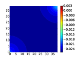
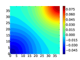
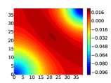
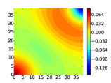
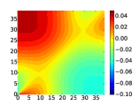
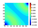
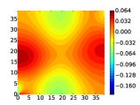
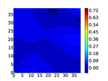
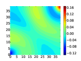
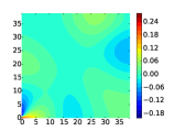
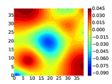
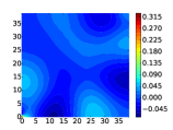
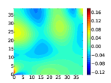
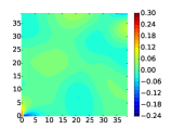
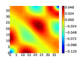
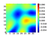
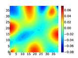
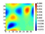
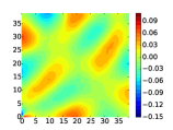
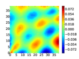
Figure 1: The first $20$ eigenvectors of the covariance kernel of $\eta_{1}$.

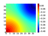
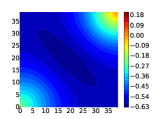
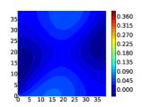
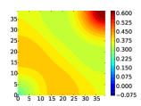
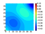
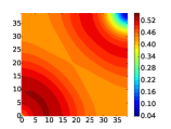
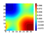
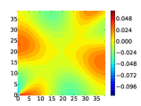
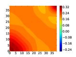
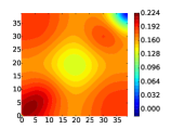
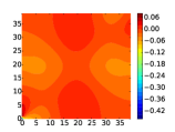
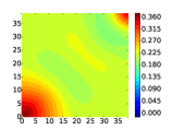
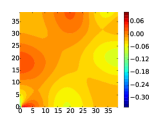
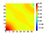
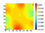
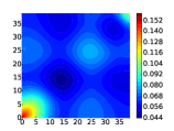
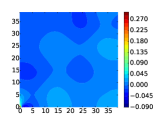
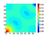
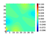
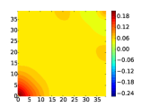
Figure 2: The $20$ entries of the first row of $\mathbf{A}(\mathbf{x})$ for the Gaussian adaptation.

3.1.1 Gaussian adaptation

First we construct the $1$-dimensional adapted $2$nd-order series

$$u^{\mathbf{A}(\mathbf{x})}(\eta)=u_{0}^{\mathbf{A}(\mathbf{x})}+u_{1}^{\mathbf{A}(\mathbf{x})}\eta+u_{2}^{\mathbf{A}(\mathbf{x})}\frac{\eta^{2}-1}{\sqrt{2}}$$ (36)

using as $\mathbf{A}(\mathbf{x})$ family of isometries where the first row is defined as in Eq. (9), that is the Gaussian adaptation. The kernel of the transformed input $\eta$, that is $k_{1}(\mathbf{x},\mathbf{y})=\mathbf{a}_{1}(\mathbf{x})\mathbf{a}_{1}(\mathbf{y})^{T}$, has $20$ strictly positive eigenvalues while the rest are zero as was proved in the previous section. As expected, $\eta$ has unit variance at each location, $k_{1}(\mathbf{x},\mathbf{x})=1$ and the covariance takes smaller values elsewhere. Its eigenvectors are shown in Fig. 1 and the entries of the first row of $\mathbf{A}(\mathbf{x})$ are shown in Fig. 2, which are essentially the normalized coefficients $\{u_{\epsilon_{i}}(\mathbf{x})\}_{i=1}^{20}$ as indicated in Eq. (9).

The coefficients in expression (36) are shown in Fig. 3. As it seems by construction, the finer scales of fluctuation that can be seen in the coefficients of the full expansion, are merged within $\eta$ and are captured by its distribution and its covariance kernel while the coefficients of the adapted expansion display only the coarse behavior. Analytically, it can be seen for instance (see Eq 79) that the first order coefficient is nothing but the norm of the first order coefficients of the full expansion. The black dots indicate $9$ locations where a comparison of the probability densities of $\{u^{\mathbf{A}(\mathbf{x}_{i})}(\eta)\}_{i=1}^{9}$ and $\{u^{\mathbf{A}(\mathbf{x}_{i})}(\eta)\}_{i=1}^{9}$ was performed, the results of which are shown in Fig. 4. The density functions of the two chaos expansions demonstrate good agreement among the two random quantities, with those of the adapted expansions being slightly more peaked and with lighter tails, due to the relatively large number of terms being essentially neglected via projection. Note that while the initial series consists of $1771$ terms, the adapted series consists of only $3$! At last, Fig. 5 shows an example of realizations of the velocity fields

$$\mathbf{v}=-\boldsymbol{\kappa}(\mathbf{x},\boldsymbol{\xi})\nabla u(\mathbf{x},\boldsymbol{\xi}),\ \ \mathbf{x}\in D$$ (37)

computed for both $u(\mathbf{x},\boldsymbol{\xi})$ and $u^{\mathbf{A}(\mathbf{x})}(\eta)$.

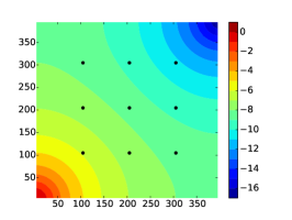
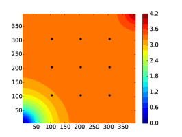
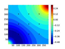
Figure 3: Coefficients $u^{\mathbf{A}(\mathbf{x})}_{i\epsilon_{1}}$, $i=0,1,2$ of the second-order one-dimensional Gaussian adaptation.

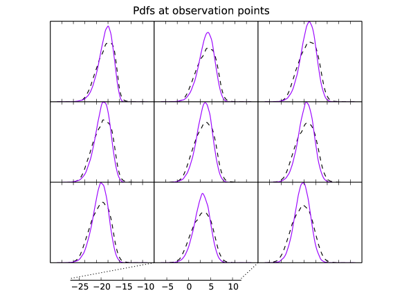
Figure 4: Gaussian adaptation: Comparison of the pdfs of $\{u(\mathbf{x}_{i},\boldsymbol{\xi})\}_{i=1}^{9}$ and $\{u^{\mathbf{A}(\mathbf{x}_{i})}(\eta)\}_{i=1}^{9}$, where $\mathbf{x}_{i}$, $i=1,...,9$ are the points of interest. The black dashed line corresponds to the original chaos expansion $u(\mathbf{x},\boldsymbol{\xi})$, while the purple line indicates the adapted chaos exansion $u^{\mathbf{A}(\mathbf{x})}(\eta)$.

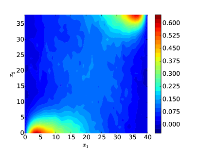
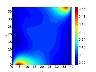
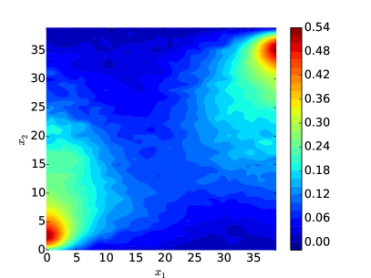
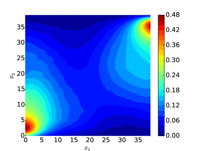
Figure 5: Sample of velocity fields $\mathbf{v}$ corresponding to $u(\mathbf{x},\boldsymbol{\xi})$ (left column) and $u^{\mathbf{A}(\mathbf{x})}(\eta)$ (right column). Top row shows $\mathbf{v}_{x_{1}}$ and bottom row shows $\mathbf{v}_{x_{2}}$.

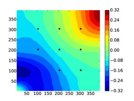
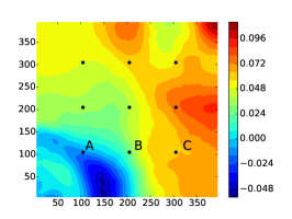
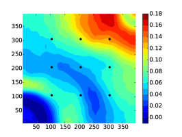
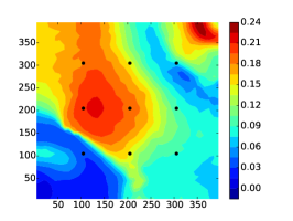
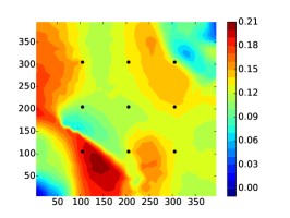
Figure 6: Coefficients $u_{ii}^{\mathbf{A}(\mathbf{x})}$, $i=1,...,5$ of the second-order $5$-dimensional quadratic adaptation.

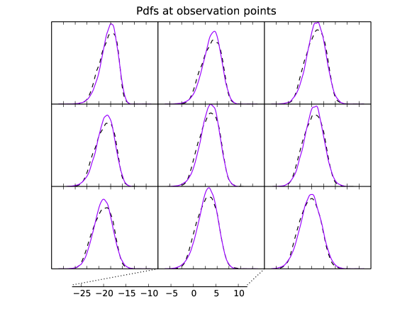
Figure 7: Quadratic adaptation: Comparison of the pdfs of $\{u(\mathbf{x}_{i},\boldsymbol{\xi})\}_{i=1}^{9}$ and $\{u^{\mathbf{A}(\mathbf{x}_{i})}(\eta)\}_{i=1}^{9}$, where $\mathbf{x}_{i}$, $i=1,...,9$ are the points of interest. The black dashed line corresponds to the original chaos expansion $u(\mathbf{x},\boldsymbol{\xi})$, while the purple line indicates the adapted chaos exansion $u^{\mathbf{A}(\mathbf{x})}(\eta)$.

3.1.2 Quadratic adaptation

Next we construct a $5$-dimensional quadratic adaptation, that is

$$u^{\mathbf{A}(\mathbf{x})}(\eta)=u_{0}^{\mathbf{A}(\mathbf{x})}+\sum_{i=1}^{5}u_{i}^{\mathbf{A}(\mathbf{x})}\eta_{i}+\sum_{i=1}^{5}u_{ii}^{\mathbf{A}(\mathbf{x})}\frac{(\eta_{i}^{2}-1)}{\sqrt{2}},$$ (38)

where $\mathbf{A}$ is constructed such that is satisfies Eq. (10). The quadratic adaptation can be seen [32] to have exactly the same sum of the polynomial terms up to order two with those of the full expansion without essentially discarding any terms via projection and the second order coefficients $u_{ii}^{\mathbf{A}(\mathbf{x})}$ are proportional to the eigenvalues of $\mathbf{S}$ (shown in Fig. 6). Due to the small order of our full expansion, this might be expexted to adapt better than the Gaussian adaptation, given also that we include an expansion with higher dimensionality than the 1-dimensional Gaussian adaptation. Comparison of the density functions at $9$ locations with those of the full expansion can be seen in Fig. 7 which verifies our argument and shows particularly a better agreement between the tails of the two pdfs. The two adaptations are also compared with themselves at three locations, labeled A, B and C (shown in $u_{22}^{\mathbf{A}(\mathbf{x})}$ - Fig. 6) and the results are shown in Fig. 8 where this time the distributions of a $5$- and $10$-dimensional Gaussian adaptations are plotted together with the $5$-dimensional quadratic adaptation. Again, good agreement can be seen between the $3$ pdfs with the quadratic adaptation being slightly closer to the true distribution. Another interesting characteristic here is that as we keep increasing the dimensionality of the expansion by adding only terms of $1$-dimensional series, that is, dropping polynomial terms that depend jointly on two or more $\xi$’s, the contribution is small and it seems that the joint terms are essential in achieving a full distributional equality (in fact the equality will be almost surely). However, the agreement shown here can be considered sufficient for estimating various statistics of interest. Further investigation in order to identify the suitable rotations to optimally adapt the expansion while maintaining low dimensionality could be pursued by minimizing an error function of the form (15),(16) or within the context of active subspaces [4] and is beyond the scope of this work.

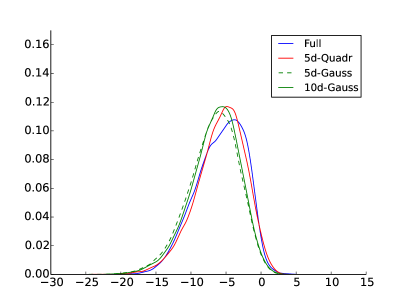
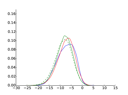
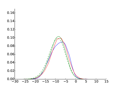
Figure 8: Comparison of the Gaussian and quadratic adaptation for different choices of the dimension at the three locations A (up left), B (up right) and C (bottom).

3.1.3 Adaptation on expansion with random coefficients

At last, we test our approach on a reduced chaos expansion with random coefficients as given in Eq. (20) where we have arbitrarily chosen $\hat{\boldsymbol{\xi}}=(\xi_{1},\xi_{2},\xi_{3},\xi_{4})$ and $\hat{\boldsymbol{\zeta}}=(\xi_{5},...,\xi_{20})$. Although this can be seen as a way to separate fine and coarse random fluctuations (and this is in fact our motivation behind this construction, as was introduced in [31]), we do not claim this to be the case here since the influence of the first four $\xi$’s is not necessarily significantly dominating in this particular permeability model due to the relatively low correlation lengths $\ell_{1}$, $\ell_{2}$. We restrict ourselves in presenting only how the adaptation methodology applies in such a case and leave the costruction of a more illustrating example for another paper. The $4$-dimensional third-order expansion with respect to $\hat{\boldsymbol{\xi}}$ with the coefficients being dependent on $\hat{\boldsymbol{\zeta}}$ is,

$$\begin{array}[]{c}u(\mathbf{x},\hat{\boldsymbol{\xi}},\hat{\boldsymbol{\zeta}})=\mathbf{U}_{0}(\mathbf{x},\hat{\boldsymbol{\zeta}})+\sum_{i=1}^{16}\mathbf{U}_{i\epsilon_{1}}(\mathbf{x},\hat{\boldsymbol{\zeta}})\psi_{i\epsilon_{1}}(\xi_{i})+\\ +\sum_{\boldsymbol{\alpha},|\boldsymbol{\alpha}|=2}\mathbf{U}_{\boldsymbol{\alpha}}(\mathbf{x},\hat{\boldsymbol{\zeta}})\psi_{\boldsymbol{\alpha}}(\hat{\boldsymbol{\xi}})+\sum_{\boldsymbol{\alpha},|\boldsymbol{\alpha}|=3}\mathbf{U}_{\boldsymbol{\alpha}}(\mathbf{x},\hat{\boldsymbol{\zeta}})\psi(\hat{\boldsymbol{\xi}})\end{array}$$ (41)

where $\mathbf{U}_{\boldsymbol{\alpha}}$ are given in Eq. (21). We use again the Gaussian adaptation scheme to construct a $1$-dimensional second order expansion

$$u^{\mathbf{A}(\boldsymbol{\zeta})}(\hat{\boldsymbol{\xi}},\eta)=\mathbf{U}^{\mathbf{A}(\mathbf{x},\boldsymbol{\zeta})}_{0}+\mathbf{U}^{\mathbf{A}(\mathbf{x},\boldsymbol{\zeta})}_{1}\eta+\mathbf{U}_{2}^{\mathbf{A}(\mathbf{x},\boldsymbol{\zeta})}\frac{\eta^{2}-1}{\sqrt{2}}$$ (42)

Note here that only the $4$-dimensional $\hat{\boldsymbol{\xi}}$ has been merged into a $1$-dimensional $\eta$ while the influence of all dimensions incorporated in $\hat{\boldsymbol{\zeta}}$ is present both in the coefficients and in the polynomials through the isometry $\mathbf{A}(\mathbf{x},\boldsymbol{\zeta})$. The estimated expected values of the adapted coefficients $\mathbf{U}_{i}^{\mathbf{A}(\mathbf{x},\boldsymbol{\zeta})}$ are shown in Fig. 9. The density functions shown in Fig. 10 are constructed by simultanesously sampling from $\hat{\boldsymbol{\zeta}}$ and $\hat{\boldsymbol{\xi}}$, then evaluating $\mathbf{U}_{\boldsymbol{\alpha}}$ and $\mathbf{A}$ based on the values of $\hat{\boldsymbol{\zeta}}$ and subsequently computing the coefficients of the adapted expansion that at last are evaluated on $\hat{\boldsymbol{\xi}}$. Again very good agreement is observed when compared to the pdfs of the full expansions. Since we have only applied the basis rotation on $4$ dimensions, upon re-expanding the series, this is a $17$-dimensional expansion.

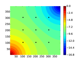
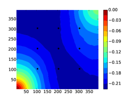
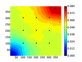
Figure 9: Expectation of the random coefficients $\mathbb{E}\left[\mathbf{U}^{\mathbf{A}(\mathbf{x},\boldsymbol{\zeta})}_{i}\right]$, $i=0,1,2$ of the second-order one-dimensional Gaussian adaptation of $u(\mathbf{x},\hat{\boldsymbol{\xi}},\hat{\boldsymbol{\zeta}})$ coefficients. As expected $\mathbb{E}\left[\mathbf{U}^{\mathbf{A}(\mathbf{x},\boldsymbol{\zeta})}_{0}\right]=u_{0}^{\mathbf{A}(\mathbf{x})}=u_{0}(\mathbf{x})$.

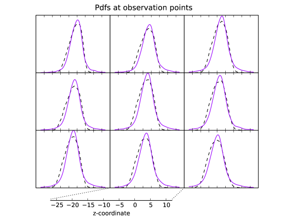
Figure 10: Adaptation with random coefficients: Comparison of the pdfs of $\{u(\mathbf{x}_{i},\boldsymbol{\xi})\}_{i=1}^{9}$ and $\{u^{\mathbf{A}(\mathbf{x}_{i})}(\eta)\}_{i=1}^{9}$, where $\mathbf{x}_{i}$, $i=1,...,9$ are the points of interest. The black dashed line corresponds to the original chaos expansion $u(\mathbf{x},\boldsymbol{\xi})$, while the purple line indicates the adapted chaos exansion $u^{\mathbf{A}(\mathbf{x})}(\eta)$.

3.2 Infinite dimensional expansion with geometric series coefficients

We consider a simple random process that is written as a function of an infinite number of Gaussians given as

$$u(x,\boldsymbol{\xi})=\sum_{n=1}^{\infty}b_{n}(x)\xi_{n}+\left(\sum_{n=1}^{\infty}b_{n}(x)\xi_{n}\right)^{2}$$ (43)

where

$$b_{n}(x)=x^{(n-1)/2},\ \ x\in(-1,1).$$ (44)

Since the sum of coefficients $b_{n}$ is square summable with $\sum_{n=1}^{\infty}b_{n}^{2}=\frac{1}{1-x}$, then $u(x,\xi)<+\infty$ a.s. for $|x|<1$ with $\sum b_{n}\xi_{n}\sim\mathcal{N}(0,\frac{1}{1-x})$ and the variance of the summand blows up for $x\to\pm 1$. We apply the $1$-dimensional Gaussian adaptation which consists of transforming $\boldsymbol{\xi}$ to

$$\eta=\frac{1}{\left(\sum_{n=1}^{\infty}b_{n}(x)^{2}\right)^{1/2}}\sum_{n=1}^{\infty}b_{n}(x)\xi_{n}$$ (45)

and using expressions (79) and (80) we take

$$u(x,\eta)=u_{1}(x)\eta+u_{2}(x)\frac{(\eta^{2}-1)}{\sqrt{2}}$$ (46)

where

$$\begin{array}[]{l}u_{1}(x)=\frac{1}{\sqrt{1-x}}\\ u_{2}(x)=\frac{1}{1+x}+\sqrt{2}\frac{x}{1-x^{2}}.\end{array}$$ (49)

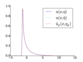
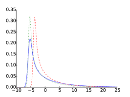
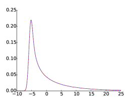
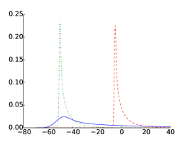
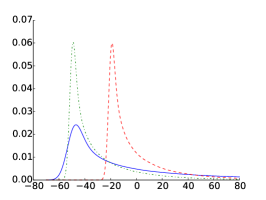
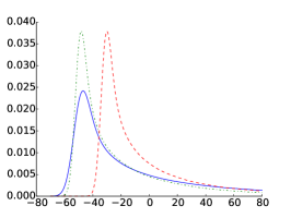
Figure 11: Top: Adaptation $u(x,\eta)$ at $x=0.3$ and its truncations using $d=10$. Middle: Adaptation at $x=0.9$ and its truncations using $d=10$ (left) and $d=50$ (middle). Bottom: Adaptation at $x=0.99$ and its truncations using $d=10$ (left), $d=50$ (middle) and $d=100$ (right).

Our goal is to compare the above analytical 1-dimensional adaptation with two truncated versions. First, the summations in the initial representation (Eq. (43)) are truncated at $d$ terms

$$u_{d}(x,\xi)=\sum_{n=1}^{d}b_{n}(x)\xi_{n}+\left(\sum_{n=1}^{d}b_{n}(x)\xi_{n}\right)^{2},$$ (50)

which after adaptation gives

$$\hat{u}_{d}(x,\eta_{d})=\hat{u}_{1}\eta_{d}+\hat{u}_{2}(x)\frac{\left(\eta_{d}^{2}-1\right)}{\sqrt{2}},$$ (51)

where

$$\begin{array}[]{l}\hat{u}_{1}(x)=\left(\frac{1-x^{d}}{1-x}\right)^{1/2}\\ \hat{u}_{2}(x)=\frac{1-x^{2d}}{(1-x^{d})(1+x)}+\frac{\sqrt{2}}{1-x^{d}}\left(\frac{x(1-x^{2d})}{1-x^{2}}-\frac{x^{d}(1-x^{d})}{1-x}\right)\end{array}$$ (54)

and

$$\eta_{d}=\frac{1}{\left(\sum_{n=1}^{d}b_{n}(x)^{2}\right)^{1/2}}\sum_{n=1}^{d}b_{n}(x)\xi_{n}.$$ (55)

Note here that $\hat{u}_{i}(x)\to u_{i}(x)$, $i=1,2$ as $d\to\infty$. Second, the adapted expansion (46) is replaced by one where only the input $\eta$ is truncated, depending only on $d$ terms, that is

$$u(x,\hat{\eta})=u_{1}(x)\hat{\eta}+u_{2}(x)\frac{(\hat{\eta}^{2}-1)}{\sqrt{2}},$$ (56)

with

$$\hat{\eta}=\frac{1}{\left(\sum_{n=1}^{\infty}b_{n}(x)^{2}\right)^{1/2}}\sum_{n=1}^{d}b_{n}(x)\xi_{n}.$$ (57)

Note that in the first truncation, although the dimensionality is initially reduced to $d$ terms, the adaptation procedure enforces $\eta$ to be standard normally distributed by construction while in the second truncation the truncated $\hat{\eta}$ is no longer standard normal (in fact it is $\mathcal{N}(0,1-x^{d})$) but it shares the same coefficients with (46).

The pdfs of the three expansions are shown in Fig. 11 for various choices of $x$ and the truncation order $d$. Although for small choices of $x$ the terms $b_{n}(x)$ decay fast and both approximations behave well, as $x$ approaches $1$, the discrepancy of $\hat{u}_{d}(x,\eta_{d})$ from $u(x,\eta)$ increases dramatically while $u(x,\hat{\eta})$ remains sufficiently close, thus making a better approximation. This illustrates the fact that a finite order truncation of the polynomial chaos expansion prior to any adaptation can behave poorly compared to a truncation that takes place after adapting the expansion. Note also that in this example the coefficients decrease geometrically and therefore their influence in the probability density of the QoI $u(x,\eta)$ vanishes rapidly. The consequences of such truncations can be even more severe in a case where all coefficients are of significant importance.

4 Conclusions

We have presented a new formulation of random processes and random fields using as starting point a homogeneous chaos expansion which allows merging the dimensions of the initial functional without deformation of its probability density structure. The tranformed input variables can be seen as an input random field with richer information about the quantity of interest than the simple standard Gaussian inputs, that we think of as an intermediate scale between the input and the chaos expansion. This novel represention has significant potential as a dimensionality reduction technique and can allow the exploration of higher dimensional polynomial chaos expansions that appear in physical systems, an area that undoubtedly has suffered a lot by the curse of dimensionality.

Appendix A Computation of the coefficients $q^{\mathbf{A}}_{\boldsymbol{\beta}}(\mathbf{x})$

A.1 Derivation of the general formula

Our goal is to derive an explicit expression for the coefficients $u^{\mathbf{A}}_{\boldsymbol{\beta}}$ defined as

$$u^{\mathbf{A}}_{\boldsymbol{\beta}}=\sum_{\boldsymbol{\alpha}\in\mathcal{J}_{p}}u_{\boldsymbol{\alpha}}\Bigl{\langle}\psi_{\boldsymbol{\alpha}}(\boldsymbol{\xi}),\psi_{\boldsymbol{\beta}}(\mathbf{A}\boldsymbol{\xi})\Bigr{\rangle},\ \ \ \boldsymbol{\beta}\in\mathcal{J}_{p}.$$ (58)

In order to prove our main result, we introduce some necessary tools that will allow us to proceed. Let $\pi_{n}:L^{2}(\Omega)\to\mathcal{G}^{\diamond n}$ be the orthogonal projection of $L^{2}(\Omega)$ onto $\mathcal{G}^{\diamond n}$. The Wick product for Gaussian variables $\xi_{i},...,\xi_{n}$ denoted with $\diamond$, is

$$\xi_{1}\diamond\cdots\diamond\xi_{n}=\pi_{n}(\xi_{1}\cdots\xi_{n})$$ (59)

that is the projection of the ordinary product $\xi_{1}\cdots\xi_{n}$ onto $\mathcal{G}^{\diamond n}$. For the case where $\xi_{1}=....=\xi_{n}$ we write $\xi^{\diamond n}=\xi_{1}\diamond\cdots\diamond\xi_{n}$. It is easy to see [19], for instance, that for $\xi\sim\mathcal{N}(0,1)$, we have $\xi^{\diamond n}=h_{n}(\xi)$ and that for any $\{\xi_{i}\}_{i=1}^{d}$ orthonormal basis in $\mathcal{G}$, $\boldsymbol{\alpha}\in\mathcal{J}$,

$$\xi_{1}^{\diamond\alpha_{1}}\diamond\cdots\diamond\xi_{d}^{\diamond\alpha_{d}}=\prod_{i=1}^{d}h_{\alpha_{i}}(\xi_{i})=h_{\boldsymbol{\alpha}}(\boldsymbol{\xi}).$$ (60)

A Feynman diagram $\gamma$ of order $n$ and rank $r$ is a graph consisting of $n$ vertices and $r$ edges such that no two edges share a common vertex. That means that there are always $2r$ paired vertices and $n-2r$ unpaired ones. The diagram is called complete when $r=n/2$. A graph where each vertex is labelled with a Gaussian random variable $\xi_{i}$, $i=1,...,n$ is said to have value

$$v(\gamma)=\prod_{k=1}^{r}\Bigl{\langle}\xi_{i_{k}},\xi_{j_{k}}\Bigr{\rangle}\prod_{i\in C}\xi_{i}$$ (61)

where $(\xi_{i_{k}},\xi_{j_{k}})$, $k=1,...,r$ are the pairs of vertices and $C$ is the set of unpaired ones. Clearly, when $\gamma$ is complete, $C$ is empty and $v(\gamma)$ is a constant. Given the above definitions, we can present the following ([19], Th. $3.12$):

Proposition 1. Let $\{\zeta_{ij}\}_{1\leq i\leq k,1\leq j\leq l_{i}}$ be real jointly Gaussian random variables and define $Y_{i}=\zeta_{i_{1}}\diamond\cdots\diamond\zeta_{i_{l_{i}}}$, then

$$\mathbb{E}\left[Y_{1}\cdots Y_{k}\right]=\sum_{\gamma}v(\gamma)$$ (62)

where the sum is taken over all complete Feynman diagrams such that no edge joins any $\zeta_{i_{1}j_{1}}$, $\zeta_{i_{2}j_{2}}$ with $i_{1}=i_{2}$.

This is also known as Wick’s theorem [34]. Taking this into account, our main result follows:

Proposition 2. Let $\{\xi_{i}\}_{i=1}^{d}$ be an orthonormal basis in $\mathcal{G}$, $A:\mathbb{R}^{d}\to\mathbb{R}^{d}$ be an isometry and take any $\boldsymbol{\alpha},\boldsymbol{\beta}\in\mathcal{J}$. Let also $\{\eta_{i}\}_{i=1}^{d}$ be such that $\boldsymbol{\eta}=A\boldsymbol{\xi}$. Then

$$\Bigl{\langle}h_{\boldsymbol{\alpha}}(\boldsymbol{\xi}),h_{\boldsymbol{\beta}}(\boldsymbol{\eta})\Bigr{\rangle}=\left\{\begin{array}[]{c}\sum_{\mathfrak{A}_{n}}\prod_{k=1}^{n}a_{i_{k},j_{k}},\ \ |\boldsymbol{\alpha}|=|\boldsymbol{\beta}|\\ 0,\ \ \ \ \ \ \ \ \ \ \ \ \ \ \ \ \ \ \ \ |\boldsymbol{\alpha}|\neq|\boldsymbol{\beta}|\end{array}\right.$$ (65)

where $a_{i_{k},j_{k}}$ are entries of $\mathbf{A}$ and the sum is taken over $\mathfrak{A}_{n}$, which is the number of possible ways to choose $n$ entries of $\mathbf{A}$ such that exactly $\alpha_{i}$ of them are in the $i$th column and $\beta_{i}$ of them are $i$th row, simultaneously, for all $i=1,...,d$.

Proof. Define $\{\zeta_{ij}\}_{1\leq i\leq k,1\leq j\leq l_{i}}$ with $k=2$, $l_{1}=|\boldsymbol{\alpha}|:=n$, $l_{2}=|\boldsymbol{\beta}|:=m$ where

$$\{\zeta_{1j}\}_{j=1}^{n}:=\left\{\underbrace{\xi_{1},...,\xi_{1}}_{\alpha_{1}},...,\underbrace{\xi_{d},...,\xi_{d}}_{\alpha_{d}}\right\},$$ (66)

$$\{\zeta_{2j}\}_{j=1}^{m}:=\left\{\underbrace{\eta_{1},...,\eta_{1}}_{\boldsymbol{\beta}_{1}},...,\underbrace{\eta_{d},...,\eta_{d}}_{\boldsymbol{\beta}_{d}}\right\}.$$ (67)

Then for $Y_{1}:=\xi_{1}^{\diamond\alpha_{1}}\diamond\cdots\diamond\xi_{d}^{\diamond\alpha_{d}}=h_{\boldsymbol{\alpha}}(\boldsymbol{\xi})$ and $Y_{2}:=\eta_{1}^{\diamond\alpha_{1}}\diamond\cdots\diamond\eta_{d}^{\diamond\alpha_{d}}=h_{\boldsymbol{\beta}}(\boldsymbol{\eta})$, Prop. 1 gives that

$$\Bigl{\langle}h_{\boldsymbol{\alpha}}(\boldsymbol{\xi}),h_{\boldsymbol{\beta}}(\boldsymbol{\eta})\Bigr{\rangle}=\mathbb{E}\left[Y_{1}Y_{2}\right]=\sum_{\gamma}v(\gamma)$$ (68)

where the sum is taken over all complete Feynman diagrams with edges that connect $\{\zeta_{1j}\}_{j=1}^{n}$ with $\{\zeta_{2j}\}_{j=1}^{m}$. Clearly for $n\neq m$ there is no such complete Feynman diagram and the sum is zero. For $n=m$, any such diagram $\gamma$ can be represented by its pairs $\left\{(\zeta_{1j},\zeta_{2l_{j}})\right\}_{j=1}^{n}$ and has value

$$v(\gamma)=\prod_{j=1}^{n}\Bigl{\langle}\zeta_{1j},\zeta_{2l_{j}}\Bigr{\rangle}=\prod_{j=1}^{\alpha_{1}}\Bigl{\langle}\xi_{1},\zeta_{2l_{j}}\Bigr{\rangle}\prod_{j=\alpha_{1}+1}^{\alpha_{1}+\alpha_{2}}\Bigl{\langle}\xi_{2},\zeta_{2l_{j}}\Bigr{\rangle}\cdots\prod_{j=n-\alpha_{d}}^{n}\Bigl{\langle}\xi_{d},\zeta_{2l_{j}}\Bigr{\rangle}.$$ (69)

Observe that any $\zeta_{2l_{j}}\in\{\eta_{s}\}_{s=1}^{d}$ and that for any $\eta_{s}$

$$\Bigl{\langle}\xi_{j},\eta_{s}\Bigr{\rangle}=\Bigl{\langle}\xi_{j},\sum_{r=1}^{d}a_{sr}\xi_{r}\Bigr{\rangle}=a_{s,j}$$ (70)

that follows from $\boldsymbol{\eta}=\mathbf{A}\boldsymbol{\xi}$ and $a_{s,j}$ is the $(s,j)$th entry of $\mathbf{A}$. Therefore, substituting in the above equation and noting that exactly $\alpha_{i}$ of the products $\Bigl{\langle}\cdot,\cdot\Bigr{\rangle}$ include $\xi_{i}$ and exactly $\beta_{i}$ include $\eta_{i}$ we obtain that exactly $\alpha_{i}$ and $\beta_{i}$ entries of $\mathbf{A}$ will be taken from the $i$th column and $i$th row respectively, which completes the proof.                                                                       $\square$

An immediate consequence of the above proposition, when one wants to compute the coefficients of a chaos expansion with respect to a rotated basis $\boldsymbol{\eta}=\mathbf{A}\boldsymbol{\xi}$, is that the sum is reduced to

$$u^{\mathbf{A}}_{\boldsymbol{\beta}}=\sum_{\boldsymbol{\alpha}\in\mathcal{J}_{p}}u_{\boldsymbol{\alpha}}\Bigl{\langle}\psi_{\boldsymbol{\alpha}}(\boldsymbol{\xi}),\psi_{\boldsymbol{\beta}}(\mathbf{A}\boldsymbol{\xi})\Bigr{\rangle}=\sum_{\boldsymbol{\alpha},|\boldsymbol{\alpha}|=|\boldsymbol{\beta}|}u_{\boldsymbol{\alpha}}\Bigl{\langle}\psi_{\boldsymbol{\alpha}}(\boldsymbol{\xi}),\psi_{\boldsymbol{\beta}}(\mathbf{A}\boldsymbol{\xi})\Bigr{\rangle}.$$ (71)

The above formula can be further simplified for the case of $1$-dimensional polynomials:

Corollary 1. For any $n\in\mathbb{N}$, $\boldsymbol{\alpha}\in\mathcal{J}$ with $|\boldsymbol{\alpha}|=n$ and $i=1,...,d$, we have

$$\Bigl{\langle}h_{\boldsymbol{\alpha}}(\boldsymbol{\xi}),h_{n}(\eta_{i})\Bigr{\rangle}=n!\prod_{k=1}^{d}a_{i,k}^{\alpha_{k}}$$ (72)

Proof. Let $\boldsymbol{\beta}\in\mathcal{J}$ with $\boldsymbol{\beta}=n\boldsymbol{\epsilon}_{i}=(0,...,n,...,0)$ and by working as in the proof of Prop. 2 with

$$\{\zeta_{2j}\}_{j=1}^{n}=\left\{\underbrace{\eta_{i},...,\eta_{i}}_{n}\right\},$$ (73)

it is easy to see that all complete Feynman diagrams take the same value, that is

$$v(\gamma)=\prod_{j=1}^{\alpha_{1}}\Bigl{\langle}\xi_{1},\eta_{i}\Bigr{\rangle}\cdots\prod_{j=1}^{\alpha_{d}}\Bigl{\langle}\xi_{d},\eta_{i}\Bigr{\rangle}=a_{i,1}^{\alpha_{i}}\cdots a_{i,d}^{\alpha_{d}}=\prod_{k=1}^{d}a_{i,k}^{\alpha_{k}}$$ (74)

and the total number of such diagrams is $n!$.                                 $\square$

A.2 Coefficients for $1$-dimensional subspaces

Taking into account Corollary 1 from the previous paragraph, we are now ready to derive explicit formulas for the coefficients along $1$-dimensional subspaces of chaos expansion $u^{\mathbf{A}}(\boldsymbol{\eta})$. Namely, for any $\boldsymbol{\beta}\in\mathcal{J}$ with $\boldsymbol{\beta}=n\boldsymbol{\epsilon}_{i}=(0,...,n,...,0)$, $i=1,...,d$ and $n\in\mathbb{N}$, we have

$$u^{\mathbf{A}}_{\boldsymbol{\beta}} = \sum_{\boldsymbol{\alpha},|\boldsymbol{\alpha}|=n}u_{\boldsymbol{\alpha}}\Bigl{\langle}\psi_{\boldsymbol{\alpha}}(\boldsymbol{\xi}),\psi_{n}(\eta_{i})\Bigr{\rangle}=$$ (75)

$$= \sum_{\boldsymbol{\alpha},|\boldsymbol{\alpha}|=n}\frac{u_{\boldsymbol{\alpha}}}{\sqrt{\boldsymbol{\alpha}!}\sqrt{n!}}\Bigl{\langle}h_{\boldsymbol{\alpha}}(\boldsymbol{\xi}),h_{n}(\eta_{i})\Bigr{\rangle}=$$ (76)

$$= \sqrt{n!}\sum_{\boldsymbol{\alpha},|\boldsymbol{\alpha}|=n}\frac{u_{\boldsymbol{\alpha}}}{\sqrt{\boldsymbol{\alpha}!}}\prod_{k=1}^{d}a_{i,k}^{\alpha_{k}}.$$ (77)

The coefficients of $\psi_{\boldsymbol{\beta}}(\boldsymbol{\eta})$ of order up to $3$ are given by:

$$u_{0}^{\mathbf{A}} = u_{0}$$ (78)

$$u_{\epsilon_{i}}^{\mathbf{A}} = \sum_{k=1}^{d}a_{i,k}u_{\epsilon_{k}}$$ (79)

$$u_{2\epsilon_{i}}^{\mathbf{A}} = \sum_{k=1}^{d}u_{kk}a_{i,k}^{2}+\sqrt{2}\sum_{\begin{subarray}{c}k=1\\ j>k\end{subarray}}^{d}u_{kj}a_{i,k}a_{i,j}$$ (80)

$$u_{3\epsilon_{i}}^{\mathbf{A}} = \sum_{k=1}^{d}u_{kkk}a_{i,k}^{3}+\sqrt{3}\sum_{\begin{subarray}{c}k=1\\ j>k\end{subarray}}^{d}u_{kkj}a_{i,k}^{2}a_{i,j}+$$ (81)

$$+ \sqrt{6}\sum_{\begin{subarray}{c}k=1\\ j>k\\ l>j\end{subarray}}^{d}u_{kjl}a_{i,k}a_{i,j}a_{i,l}$$ (82)

Appendix B Proof of Theorem 1

We have

$$\int_{D}\int_{D}|k_{i}(\mathbf{x},\mathbf{y})|^{2}d\mathbf{x}d\mathbf{y}=$$

$$=\sum_{j,k=1}^{d}\int_{D}a_{ij}(\mathbf{x})a_{ik}(\mathbf{x})d\mathbf{x}\int_{D}a_{ij}(\mathbf{y})a_{ik}(\mathbf{y})d\mathbf{y}\leq$$

$$\leq\sum_{j,k=1}^{d}||a_{ij}||^{2}_{L^{2}(D)}||a_{ik}||^{2}_{L^{2}(D)}<+\infty$$

where the second row is derived after applying the Cauchy-Schwarz inequality.

Appendix C Proof of Lemma 1

Clearly by definition $\eta(\mathbf{x})\in\mathcal{G}$ for all $\mathbf{x}\in D$ since $\{\xi_{i}\}_{i\in\mathbb{N}}$ forms a basis in $\mathcal{G}$, therefore $span\{\eta(\mathbf{x})\}_{\mathbf{x}\in D}\subset\mathcal{G}$. On the oher hand, for any $\xi\in\mathcal{G}$ there exists $\chi\in H$ such that

$$\xi=\Bigl{\langle}\chi,\boldsymbol{\xi}\Bigr{\rangle}_{H}=\sum_{i}\chi_{i}\xi_{i}$$ (83)

where $\chi_{n}=\langle\chi,\mathbf{e}_{n}\rangle_{H}$ with $\{\mathbf{e}_{n}\}_{n\in\mathbb{N}}$ some basis in $H$. Set $\mathbf{x}_{1}\in\mathcal{A}^{-1}\left(\{\mathbf{e}_{n}\}_{n\in\mathbb{N}}\right)$ and for $n\geq 2$ choose $\mathbf{x}_{n}$ such that $\mathbf{e}_{n}=\hat{\mathbf{e}}_{1}(\mathbf{x}_{n})$ where $\hat{\mathbf{e}}_{1}(\mathbf{x}_{n})$ is the first basis element of $\mathcal{A}(\mathbf{x}_{n})$. This is possible since we can continuously rotate any basis until its $n$-th element becomes the first element of another basis. Then

$$\xi = \Bigl{\langle}\chi,\boldsymbol{\xi}\Bigr{\rangle}_{H}=\sum_{i}\Bigl{\langle}\chi_{i},\mathbf{e}_{i}\Bigr{\rangle}_{H}\Bigl{\langle}\mathbf{e}_{i},\boldsymbol{\xi}\Bigr{\rangle}_{H}$$

$$= \sum_{i}\chi_{i}\Bigl{\langle}\mathbf{e}(\mathbf{x}_{i}),\mathbf{x}\Bigr{\rangle}_{H}=\sum_{i}\chi_{i}\eta(\mathbf{x}_{i}),$$

therefore $\xi\in span\{\eta(\mathbf{x})\}_{\mathbf{x}\in D}$ and $\mathcal{G}\subset span\{\eta(\mathbf{x})\}_{\mathbf{x}\in D}$ which completes the proof.

Appendix D Proof of Theorem 2

It is known ([19], Theorem $8.15$) that the linear mapping $R_{\eta}(\cdot)(\mathbf{x})$ is an isometry from $span\{\eta(\mathbf{x})\}_{\mathbf{x}\in D}$ to $\mathcal{R}_{\eta}(\mathcal{G})$ and by using Lemma 1 we have that $\mathcal{G}$ and $\mathcal{R}_{\eta}(\mathcal{G})$ have the same dimension. Also ([19], Corollary $8.16$) $\mathcal{R}_{\eta}(\mathcal{G})$ is spanned by the covariance kernels

$$k_{\mathbf{y}}(\mathbf{x})=\mathcal{R}_{\eta}(\eta(\mathbf{y}))(\mathbf{x})=\mathbb{E}[\eta(\mathbf{y})\eta(\mathbf{x})],\ \ \ \mathbf{y}\in D$$ (84)

and ([19], Theorem $8.22$) $\eta(\mathbf{x})$ admits a representation

$$\eta(\mathbf{x})=\sum_{i=1}^{\infty}\rho_{i}(\mathbf{x})\xi_{i}$$ (85)

where $\{\rho_{i}\}_{i\in\mathbb{N}}$ is a basis in $\mathcal{R}_{\eta}(\mathcal{G})$ and $\{\xi_{i}\}$ a basis in $span\{\eta(\mathbf{x})\}_{\mathbf{x}\in D}=\mathcal{G}$ and the limit is taken in $L^{2}$. Let $\{\mathbf{y}_{i}\}_{i\in\mathbb{N}}$ such that $\rho^{i}(\mathbf{x})=k_{\mathbf{y}_{i}}(\mathbf{x})$. From the proof of Lemma 1 we can see that it is possible to choose $\mathbf{y}_{i}$ such that $\eta(\mathbf{y}_{i})=\xi_{i}$, all $i\in\mathbb{N}$. That is due to the fact that the isometry $R_{\eta}(\cdot)(\mathbf{x})$ will map the basis $\{\eta(\mathbf{y}_{i})\}_{i\in\mathbb{N}}$ to a basis $\{k_{\mathbf{y}_{i}}(\mathbf{x})\}_{i\in\mathbb{N}}$ in $\mathcal{R}_{\eta}(\mathcal{G})$. Then

$$\eta(\mathbf{x}) = \sum_{i}\rho_{i}(\mathbf{x})\xi_{i}=\sum_{i}k_{\mathbf{y}_{i}}(\mathbf{x})\xi_{i}=\sum_{i}\mathbb{E}[\xi_{i}\eta(\mathbf{x})]\xi_{i}$$

$$= \sum_{i}\Bigl{\langle}\xi_{i},\eta(\mathbf{x})\Bigr{\rangle}_{\mathcal{G}}\xi_{i}=\sum_{i}\sum_{j}e^{j}(\mathbf{x})\Bigl{\langle}\xi_{i},\xi_{j}\Bigr{\rangle}_{\mathcal{G}}\xi_{i}$$

$$= \sum_{i}e^{i}(\mathbf{x})\xi_{i},$$

from where we obtain $\rho^{i}(\mathbf{x})=e^{i}(\mathbf{x})$.

References

- [1] J. Aarnes, T. Gimse, and K.-A. Lie. An introduction to the numerics of flow in porous media using matlab. Geometric Modelling, Numerical Simulation and Optimization, pages 265–306, 2007.
- [2] M. Arnst, R. Ghanem, and C. Soize. Identification of bayesian posteriors for coefficients of chaos expansions. Journal of Computational Physics, 229:3134–3154, 2010.
- [3] R. Cameron and W. Martin. The orthogonal development of nonlinear functionals in series of fourier-hermite functionals. Annals of Mathematics, 48:385–392, 1947.
- [4] P. G. Constantine, E. Dow, and Q. Wang. Active subspace methods in theory and practice: applications to kriging surfaces. SIAM Journal on Scientific Computing, 36:A1500–A1524, 2014.
- [5] S. Das, R. Ghanem, and J.C. Spall. Asymptotic sampling distribution for polynomial chaos representation from data: a maximum entropy and fisher information approach. SIAM Journal on Scientific Computing, 30:2207–2234, 2008.
- [6] C. Desceliers, R. Ghanem, and C. Soize. Maximum likelihood estimation of stochastic chaos representations from experimental data. International Journal for Numerical Methods in Engineering, 66:978–1001, 2006.
- [7] A. Doostan and G. Iaccarino. A least-squares approximation of partial differential equations with high-dimensional random inputs. Journal of Computational Physics, 228:4332–4345, 2009.
- [8] A. Doostan and H. Owhadi. A non-adapted sparse approximation of pdes with stochastic inputs. Journal of Computational Physics, 230:3015–3034, 2011.
- [9] I.M. Gelfand and N. Ya. Vilenkin. Generalized functions, Vol 4: Applications to Harmonic Analysis. Academic Press, 1964.
- [10] R. Ghanem. Scales of fluctuation and the propagation of uncertainty in random porous media. Water Resources Research, 34:2123–2136, 1998.
- [11] R. Ghanem. Ingredients for a general purpose stochastic finite elements implementation. Computer Methods in Applied Mechanics and Engineering, 168:19–34, 1999.
- [12] R. Ghanem and S. Dham. Stochastic finite element analysis for multiphase flow in heterogeneous porous media. Transport in Porous Media, 32:239–262, 1998.
- [13] R. Ghanem and R. Doostan. Characterization of stochastic system parameters from experimental data: A bayesian inference approach. Journal of Computational Physics, 217:63–81, 2006.
- [14] R. Ghanem and J. Red-Horse. Propagation of probabilistic uncertainty in complex physical systems using a stochastic finite element approach. Physica D: Nonlinear Phenomena, 133:137–144, 1999.
- [15] R. Ghanem and P. Spanos. Stochastic finite elements: A spectral approach. Springer-Verlag, 1991.
- [16] R.G. Ghanem, A. Doostan, and J. Red-Horse. A probabilistic construction of model validation. Computer Methods in Applied Mechanics and Engineering, 197:2585–2595, 2008.
- [17] X. Huan and Y.M. Marzouk. Simulation-based optimal bayesian experimental design for nonlinear systems. Journal of Computational Physics, 232:288–317, 2013.
- [18] K. Itô. An elementary approach to malliavin fields. In Asymptotic problems in probability theory: Wiener functionals and asymptotics, pages 35–89, Essex, 1990. Sanda and Kyoto.
- [19] S. Janson. Gaussian Hilbert spaces. Cambridge University Press, 1999.
- [20] K. Karhunen. Über lineare methoden in der wahrscheinlichkeits-rechnung. Annals of Academic Science Fennicade Series A1, Mathematical Physics, 37:3–79, 1946.
- [21] O.P. Le Maître, M.T. Reagan, H.N. Najm, R.G. Ghanem, and O.M. Knio. A stochastic projection method for fluid flow: Ii. random process. Journal of Computational Physics, 181:9–44, 2002.
- [22] M. Loéve. Probability Theory, D. Van Nostrand, Princeton, New Jersey, 1955.
- [23] Y. M. Marzouk, H. N. Najm, and L. Rahn. Stochastic spectral methods for efficient bayesian solution of inverse problems. Journal of Computational Physics, 224:560–586, 2007.
- [24] Y.M. Marzouk and H.N. Najm. Dimensionality reduction and polynomial chaos acceleration of bayesian inference in inverse problems. Journal of Computational Physics, 228:1862–1902, 2009.
- [25] H.G. Matthies and C. Bucher. Finite elements for stochastic media problems. Computer Methods in Applied Mechanics and Engineering, 168:3–17, 1999.
- [26] J. Mercer. Functions of positive and negative type, and their connection with the theory of integral equations. Philosophical Transactions of the Royal Society of London. Series A, containing papers of a mathematical or physical character, 209:415–446, 1909.
- [27] H.N. Najm. Uncertainty quantification and polynomial chaos techniques in computational fluid dynamics. Annual Review of Fluid Mechanics, 41:35–52, 2009.
- [28] J. Red-Horse and R. Ghanem. Elements of a functional analytic approach to probability. International Journal for Numerical Methods in Engineering, 80(6-7):689–716, 2009.
- [29] G. Saad and R. Ghanem. Characterization of reservoir simulation models using a polynomial chaos-based ensemble kalman filter. Water Resources Research, 45:Art. W04417, 2009.
- [30] C. Soize and R. Ghanem. Physical systems with random uncertainties: chaos representations with arbitrary probability measure. SIAM Journal on Scientific Computing, 26:395–410, 2004.
- [31] C. Soize and R. Ghanem. Reduced chaos decomposition with random coefficients of vector-valued random variables and random fields. Computer Methods in Applied Mechanics and Engineering, 198:1926–1934, 2009.
- [32] R. Tipireddy and R.G. Ghanem. Basis adaptation in homogeneous chaos spaces. Journal of Computational Physics, 259:304–317, 2014.
- [33] P. Tsilifis, R.G. Ghanem, and P. Hajali. Efficient bayesian experimentation using an expected information gain lower bound. arXiv preprint, arXiv:1506.00053v2, 2015.
- [34] G.C. Wick. The evaluation of the collision matrix. Physical Review, 80:268–272, 1950.
- [35] N. Wiener. The homogeneous chaos. American Journal of Mathematics, 60:897–936, 1938.
- [36] D. Xiu and G.E. Karniadakis. The wiener–askey polynomial chaos for stochastic differential equations. SIAM Journal on Scientific Computing, 24:619–644, 2002.
- [37] D. Xiu and G.E. Karniadakis. Modeling uncertainty in flow simulations via generalized polynomial chaos. Journal of Computational Physics, 187:137–167, 2003.