Nonlinear Spinor Fields in Bianchi type-III spacetime

Abstract

Within the scope of Bianchi type-III spacetime we study the role of spinor field on the evolution of the Universe as well as the influence of gravity on the spinor field. In doing so we have considered a polynomial type of nonlinearity. In this case the spacetime remains locally rotationally symmetric and anisotropic all the time. It is found that depending on the sign of nonlinearity the models allows both accelerated and oscillatory modes of expansion. The non-diagonal components of energy-momentum tensor though impose some restrictions on metric functions and components of spinor field, unlike Bianchi type I, V and $VI_{0}$ cases, they do not lead to vanishing mass and nonlinear terms of the spinor field.

I Introduction

Discovery and further reconfirmation of the existence of the late time accelerated mode of expansion riess ; perlmutter have given rise to a number of alternative studies of the evolution of the Universe.

Though the models with $\Lambda$-term starobinsky ; PRpadma ; 2006APSS302-83-91 , quintessence Carden ; chimento1 ; Linder1 ; olivares ; zlatev ; 2005ChineseJPhys43-1035-1043 , Chaplygin gas Kamenshchik ; Amendola ; Bean ; bento ; B1 ; B2 ; B4 ; bilic etc. retain their position as the prime candidates to explain this phenomenon, nevertheless some other models of dark energy are also proposed. After some remarkable works by different authors henneaux ; ochs ; saha1997a ; saha1997b ; saha2001a ; greene ; saha2004a ; saha2004b ; ribas ; saha2006c ; saha2006e ; saha2007 ; saha2006d ; souza ; kremer , showing the important role of spinor field in the evolution of the Universe, it has been extensively used to model the dark energy. This success is directly related to its ability to answer some fundamental questions of modern cosmology: (i) Problem of initial singularity and its possible elimination saha1997a ; saha1997b ; saha2001a ; saha2004a ; saha2004b ; PopPLB ; PopPRD ; PopGREG ; FabIJTP ; (ii) problem of isotropization misner ; saha2001a ; saha2004a ; saha2006c ; PopPRD and (iii) late time acceleration of the Universe ribas ; saha2006d ; saha2006e ; saha2007 ; PopGREG ; PopPLB ; FabIJTP ; ELKO ; FabJMP ; PopPRD . Moreover recently it was found that the spinor field can also describe the different characteristics of matter from ekpyrotic matter to phantom matter, as well as Chaplygin gas krechet ; saha2010a ; saha2010b ; saha2011 ; saha2012 .

In some recent studies sahaIJTP2014 ; sahaAPSS2015 ; sahabvi0 it was shown that due to its specific behavior in curve spacetime the spinor field can significantly change not only the geometry of spacetime but itself as well. The existence of nontrivial non-diagonal components of the energy-momentum tensor plays a vital role in this matter. In sahaIJTP2014 ; sahaAPSS2015 it was shown that depending on the type restriction imposed on the non-diagonal components of the energy-momentum tensor, the initially Bianchi type-I evolve into a LRS Bianchi type-I spacetime or FRW one from the very beginning, whereas the model may describe a general Bianchi type-I spacetime but in that case the spinor field becomes massless and linear. The same thing happens for a Bianchi type-$VI_{0}$ spacetime, i.e., the geometry of Bianchi type-$VI_{0}$ spacetime does not allow the existence of a massive and nonlinear spinor field in some particular cases sahabvi0 . In this paper we study the role of spinor field on the evolution of a Bianchi type-III spacetime.

The purpose of considering the anisotropic cosmological models lies on the fact that recent observational data from Cosmic Background Explorer’s differential Radiometer have detected and measured cosmic microwave background anisotropies in different angular scale. We consider here Bianchi type III model due to some special interest of cosmologist towards it due to its peculiar geometric interpretation Coley . Yadav et al. YadavMK , Pradhan et al. PAZ ; PLA have recently studied homogeneous and anisotropic Bianchi type-III spacetime in context of massive strings. Recently Yadav YadavYadav has obtained Bianchi type-III anisotropic DE models with constant deceleration parameter. In this paper, they have investigated a new anisotropic Bianchi type-III DE model with variable $\omega$ without assuming constant deceleration parameter. A spinor description of dark energy within the scope of a BIII model was given in 2012IJTP51-1812-1837 . Further the accelerating dark energy models of the Universe within the scope of Bianchi type-III spacetime were studied in 2014EChAYa45-349-396 ; 2015EChAYa46-310-346 ; Akarsu . Bianchi type III cosmological models with varying $\Lambda$ term was studied in Adhav .

II Basic equation

Let us consider the case when the anisotropic spacetime is filled with nonlinear spinor field. The corresponding action can be given by

$${\cal S}(g;\psi,\bar{\psi})=\int\,L\sqrt{-g}d\Omega$$ (1)

with

$$L=L_{\rm g}+L_{\rm sp}.$$ (2)

Here $L_{\rm g}$ corresponds to the gravitational field

$$L_{\rm g}=\frac{R}{2\kappa},$$ (3)

where $R$ is the scalar curvature, $\kappa=8\pi G$, with $G$ being Newton’s gravitational constant and $L_{\rm sp}$ is the spinor field Lagrangian.

II.1 Gravitational field

The gravitational field in our case is given by a Bianchi type-III anisotropic spacetime:

$$ds^{2}=dt^{2}-a_{1}^{2}e^{-2mx_{3}}dx_{1}^{2}-a_{2}^{2}dx_{2}^{2}-a_{3}^{2}dx_{3}^{2},$$ (4)

with $a_{1},\,a_{2}$ and $a_{3}$ being the functions of time only and $m$ is some arbitrary constant.

The nontrivial Christoffel symbols for (4) are

$$\Gamma_{01}^{1} = \frac{\dot{a_{1}}}{a_{1}},\quad\Gamma_{02}^{2}=\frac{\dot{a_{2}}}{a_{2}},\quad\Gamma_{03}^{3}=\frac{\dot{a_{3}}}{a_{3}},$$

$$\Gamma_{11}^{0} = a_{1}\dot{a_{1}}e^{-2mx_{3}},\quad\Gamma_{22}^{0}=a_{2}\dot{a_{2}},\quad\Gamma_{33}^{0}=a_{3}\dot{a_{3}},$$ (5)

$$\Gamma_{31}^{1} = -m,\quad\Gamma_{11}^{3}=\frac{ma_{1}^{2}}{a_{3}^{2}}e^{-2mx_{3}}.$$

The nonzero components of the Einstein tensor corresponding to the metric (4) are

$$G_{1}^{1} = -\frac{\ddot{a}_{2}}{a_{2}}-\frac{\ddot{a}_{3}}{a_{3}}-\frac{\dot{a}_{2}}{a_{2}}\frac{\dot{a}_{3}}{a_{3}},$$ (6a)

$$G_{2}^{2} = -\frac{\ddot{a}_{3}}{a_{3}}-\frac{\ddot{a}_{1}}{a_{1}}-\frac{\dot{a}_{3}}{a_{3}}\frac{\dot{a}_{1}}{a_{1}}+\frac{m^{2}}{a_{3}^{2}},$$ (6b)

$$G_{3}^{3} = -\frac{\ddot{a}_{1}}{a_{1}}-\frac{\ddot{a}_{2}}{a_{2}}-\frac{\dot{a}_{1}}{a_{1}}\frac{\dot{a}_{2}}{a_{2}},$$ (6c)

$$G_{0}^{0} = -\frac{\dot{a}_{1}}{a_{1}}\frac{\dot{a}_{2}}{a_{2}}-\frac{\dot{a}_{2}}{a_{2}}\frac{\dot{a}_{3}}{a_{3}}-\frac{\dot{a}_{3}}{a_{3}}\frac{\dot{a}_{1}}{a_{1}}+\frac{m^{2}}{a_{3}^{2}},$$ (6d)

$$G_{3}^{0} = m\left(\frac{\dot{a}_{3}}{a_{3}}-\frac{\dot{a}_{1}}{a_{1}}\right).$$ (6e)

II.2 Spinor field

For a spinor field $\psi$, the symmetry between $\psi$ and $\bar{\psi}$ appears to demand that one should choose the symmetrized Lagrangian kibble . Keeping this in mind we choose the spinor field Lagrangian as saha2001a :

$$L_{\rm sp}=\frac{\imath}{2}\biggl{[}\bar{\psi}\gamma^{\mu}\nabla_{\mu}\psi-\nabla_{\mu}\bar{\psi}\gamma^{\mu}\psi\biggr{]}-m_{\rm sp}\bar{\psi}\psi-F,$$ (7)

where the nonlinear term $F$ describes the self-interaction of a spinor field and can be presented as some arbitrary functions of invariants generated from the real bilinear forms of a spinor field. Here we consider $F=F(K)$ with $K$ being one of the following expressions:$\{I,\,J,\,I+J,\,I-J\}$, where $I=S^{2}=\left(\bar{\psi}\psi\right)^{2}$ and $J=P^{2}=\left(\imath\bar{\psi}\gamma^{5}\psi\right)^{2}.$ It can be shown that thanks to Fierz identity this type of nonlinear term describes the nonlinearity in its most general form. In (7) $\nabla_{\mu}$ is the covariant derivative of spinor field:

$$\nabla_{\mu}\psi=\frac{\partial\psi}{\partial x^{\mu}}-\Gamma_{\mu}\psi,\quad\nabla_{\mu}\bar{\psi}=\frac{\partial\bar{\psi}}{\partial x^{\mu}}+\bar{\psi}\Gamma_{\mu},$$ (8)

with $\Gamma_{\mu}$ being the spinor affine connection. In (7) $\gamma$’s are the Dirac matrices in curve spacetime and obey the following algebra

$$\gamma^{\mu}\gamma^{\nu}+\gamma^{\nu}\gamma^{\mu}=2g^{\mu\nu}$$ (9)

and are connected with the flat spacetime Dirac matrices $\bar{\gamma}$ in the following way

$$g_{\mu\nu}(x)=e_{\mu}^{a}(x)e_{\nu}^{b}(x)\eta_{ab},\quad\gamma_{\mu}(x)=e_{\mu}^{a}(x)\bar{\gamma}_{a}$$ (10)

where $e_{\mu}^{a}$ is a set of tetrad 4-vectors.

For the metric (4) we choose the tetrad as follows:

$$e_{0}^{(0)}=1,\quad e_{1}^{(1)}=a_{1}e^{-mx_{3}},\quad e_{2}^{(2)}=a_{2},\quad e_{3}^{(3)}=a_{3}.$$ (11)

The Dirac matrices $\gamma^{\mu}(x)$ of Bianchi type-III spacetime are connected with those of Minkowski one as follows:

$$\gamma^{0}=\bar{\gamma}^{0},\quad\gamma^{1}=\frac{e^{mx_{3}}}{a_{1}}\bar{\gamma}^{1},\quad\gamma^{2}=\frac{1}{a_{2}}\bar{\gamma}^{2},\quad\gamma^{3}=\frac{1}{a_{3}}\bar{\gamma}^{3}$$

$$\gamma^{5}=-\imath\sqrt{-g}\gamma^{0}\gamma^{1}\gamma^{2}\gamma^{3}=-\imath\bar{\gamma}^{0}\bar{\gamma}^{1}\bar{\gamma}^{2}\bar{\gamma}^{3}=\bar{\gamma}^{5}$$

with

$$\bar{\gamma}^{0}\,=\,\left(\begin{array}[]{cc}I&0\\ 0&-I\end{array}\right),\quad\bar{\gamma}^{i}\,=\,\left(\begin{array}[]{cc}0&\sigma^{i}\\ -\sigma^{i}&0\end{array}\right),\quad\gamma^{5}=\bar{\gamma}^{5} = \left(\begin{array}[]{cc}0&-I\\ -I&0\end{array}\right),$$ (18)

where $\sigma_{i}$ are the Pauli matrices:

$$\sigma^{1}\,=\,\left(\begin{array}[]{cc}0&1\\ 1&0\end{array}\right),\quad\sigma^{2}\,=\,\left(\begin{array}[]{cc}0&-\imath\\ \imath&0\end{array}\right),\quad\sigma^{3}\,=\,\left(\begin{array}[]{cc}1&0\\ 0&-1\end{array}\right).$$ (25)

Note that the $\bar{\gamma}$ and the $\sigma$ matrices obey the following properties:

$$\bar{\gamma}^{i}\bar{\gamma}^{j}+\bar{\gamma}^{j}\bar{\gamma}^{i}=2\eta^{ij},\quad i,j=0,1,2,3$$

$$\bar{\gamma}^{i}\bar{\gamma}^{5}+\bar{\gamma}^{5}\bar{\gamma}^{i}=0,\quad(\bar{\gamma}^{5})^{2}=I,\quad i=0,1,2,3$$

$$\sigma^{j}\sigma^{k}=\delta_{jk}+i\varepsilon_{jkl}\sigma^{l},\quad j,k,l=1,2,3$$

where $\eta_{ij}=\{1,-1,-1,-1\}$ is the diagonal matrix, $\delta_{jk}$ is the Kronekar symbol and $\varepsilon_{jkl}$ is the totally antisymmetric matrix with $\varepsilon_{123}=+1$.

The spinor affine connection matrices $\Gamma_{\mu}(x)$ are uniquely determined up to an additive multiple of the unit matrix by the equation

$$\frac{\partial\gamma_{\nu}}{\partial x^{\mu}}-\Gamma_{\nu\mu}^{\rho}\gamma_{\rho}-\Gamma_{\mu}\gamma_{\nu}+\gamma_{\nu}\Gamma_{\mu}=0,$$ (26)

with the solution

$$\Gamma_{\mu}=\frac{1}{4}\bar{\gamma}_{a}\gamma^{\nu}\partial_{\mu}e^{(a)}_{\nu}-\frac{1}{4}\gamma_{\rho}\gamma^{\nu}\Gamma^{\rho}_{\mu\nu}.$$ (27)

From the Bianchi type-VI metric (27) one finds the following expressions for spinor affine connections:

$$\Gamma_{0} = 0,$$ (28a)

$$\Gamma_{1} = \frac{1}{2}\Bigl{(}\dot{a}_{1}\bar{\gamma}^{1}\bar{\gamma}^{0}-m\frac{a_{1}}{a_{3}}\bar{\gamma}^{1}\bar{\gamma}^{3}\Bigr{)}e^{-mx_{3}},$$ (28b)

$$\Gamma_{2} = \frac{1}{2}\dot{a}_{2}\bar{\gamma}^{2}\bar{\gamma}^{0},$$ (28c)

$$\Gamma_{3} = \frac{1}{2}\dot{a}_{3}\bar{\gamma}^{3}\bar{\gamma}^{0}.$$ (28d)

II.3 Field equations

Variation of (1) with respect to the metric function $g_{\mu\nu}$ gives the Einstein field equation

$$G_{\mu}^{\nu}=R_{\mu}^{\nu}-\frac{1}{2}\delta_{\mu}^{\nu}R=-\kappa T_{\mu}^{\nu},$$ (29)

where $R_{\mu}^{\nu}$ and $R$ are the Ricci tensor and Ricci scalar, respectively. Here $T_{\mu}^{\nu}$ is the energy momentum tensor of the spinor field.

Varying (7) with respect to $\bar{\psi}(\psi)$ one finds the spinor field equations:

$$\imath\gamma^{\mu}\nabla_{\mu}\psi-m_{\rm sp}\psi-{\cal D}\psi-\imath{\cal G}\gamma^{5}\psi = 0,$$ (30a)

$$\imath\nabla_{\mu}\bar{\psi}\gamma^{\mu}+m_{\rm sp}\bar{\psi}+{\cal D}\bar{\psi}+\imath{\cal G}\bar{\psi}\gamma^{5} = 0,$$ (30b)

where we denote ${\cal D}=2SF_{K}K_{I}$ and ${\cal G}=2PF_{K}K_{J}$, with $F_{K}=dF/dK$, $K_{I}=dK/dI$ and $K_{J}=dK/dJ.$ In view of (30) the spinor field Lagrangian (7) can be rewritten as

$$L_{\rm sp} = \frac{\imath}{2}\bigl{[}\bar{\psi}\gamma^{\mu}\nabla_{\mu}\psi-\nabla_{\mu}\bar{\psi}\gamma^{\mu}\psi\bigr{]}-m_{\rm sp}\bar{\psi}\psi-F(I,\,J)$$ (31)

$$= \frac{\imath}{2}\bar{\psi}[\gamma^{\mu}\nabla_{\mu}\psi-m_{\rm sp}\psi]-\frac{\imath}{2}[\nabla_{\mu}\bar{\psi}\gamma^{\mu}+m_{\rm sp}\bar{\psi}]\psi-F(I,\,J),$$

$$= 2(IF_{I}+JF_{J})-F=2KF_{K}-F(K).$$

II.4 Energy momentum tensor of the spinor field

The energy-momentum tensor of the spinor field is given by

$$T_{\mu}^{\rho}=\frac{\imath}{4}g^{\rho\nu}\biggl{(}\bar{\psi}\gamma_{\mu}\nabla_{\nu}\psi+\bar{\psi}\gamma_{\nu}\nabla_{\mu}\psi-\nabla_{\mu}\bar{\psi}\gamma_{\nu}\psi-\nabla_{\nu}\bar{\psi}\gamma_{\mu}\psi\biggr{)}\,-\delta_{\mu}^{\rho}L_{\rm sp}.$$ (32)

Then in view of (8) and (31) the energy-momentum tensor of the spinor field can be written as

$$T_{\mu}^{\,\,\,\rho} = \frac{\imath}{4}g^{\rho\nu}\bigl{(}\bar{\psi}\gamma_{\mu}\partial_{\nu}\psi+\bar{\psi}\gamma_{\nu}\partial_{\mu}\psi-\partial_{\mu}\bar{\psi}\gamma_{\nu}\psi-\partial_{\nu}\bar{\psi}\gamma_{\mu}\psi\bigr{)}$$ (33)

$$- \frac{\imath}{4}g^{\rho\nu}\bar{\psi}\bigl{(}\gamma_{\mu}\Gamma_{\nu}+\Gamma_{\nu}\gamma_{\mu}+\gamma_{\nu}\Gamma_{\mu}+\Gamma_{\mu}\gamma_{\nu}\bigr{)}\psi\,-\delta_{\mu}^{\rho}\bigl{(}2KF_{K}-F(K)\bigr{)}.$$

As is seen from (33), is case if for a given metric $\Gamma_{\mu}$’s are different, there arise nontrivial non-diagonal components of the energy momentum tensor.

We consider the case when the spinor field depends on $t$ only. Then after a little manipulations from (33) for the components of the energy momentum tensor one finds:

$$T_{0}^{0} = m_{\rm sp}S+F(K),$$ (34a)

$$T_{1}^{1} = T_{2}^{2}=T_{3}^{3}=F(K)-2KF_{K},$$ (34b)

$$T_{1}^{0} = 0,$$ (34c)

$$T_{2}^{0} = -\frac{\imath}{4}m\frac{a_{2}}{a_{3}}\,\bar{\psi}\bar{\gamma}^{2}\bar{\gamma}^{3}\bar{\gamma}^{0}\psi=-\frac{1}{4}m\frac{a_{2}}{a_{3}}\,A^{1},$$ (34d)

$$T_{3}^{0} = 0,$$ (34e)

$$T_{2}^{1} = \frac{\imath}{4}\frac{a_{2}}{a_{1}}e^{mx_{3}}\biggl{[}\biggl{(}\frac{\dot{a}_{1}}{a_{1}}-\frac{\dot{a}_{2}}{a_{2}}\biggr{)}\bar{\psi}\bar{\gamma}^{1}\bar{\gamma}^{2}\bar{\gamma}^{0}\psi-\frac{m}{a_{3}}\bar{\psi}\bar{\gamma}^{1}\bar{\gamma}^{2}\bar{\gamma}^{3}\psi\biggr{]}$$ (34f)

$$= \frac{1}{4}\frac{a_{2}}{a_{1}}e^{mx_{3}}\biggl{[}\biggl{(}\frac{\dot{a}_{1}}{a_{1}}-\frac{\dot{a}_{2}}{a_{2}}\biggr{)}A^{3}-\frac{m}{a_{3}}A^{0}\biggr{]},$$

$$T_{3}^{1} = \frac{\imath}{4}\frac{a_{3}}{a_{1}}e^{mx_{3}}\biggl{(}\frac{\dot{a}_{3}}{a_{3}}-\frac{\dot{a}_{1}}{a_{1}}\biggr{)}\bar{\psi}\bar{\gamma}^{3}\bar{\gamma}^{1}\bar{\gamma}^{0}\psi=\frac{1}{4}\frac{a_{3}}{a_{1}}e^{mx_{3}}\biggl{(}\frac{\dot{a}_{3}}{a_{3}}-\frac{\dot{a}_{1}}{a_{1}}\biggr{)}A^{2}$$ (34g)

$$T_{3}^{2} = \frac{\imath}{4}\frac{a_{3}}{a_{2}}\biggl{(}\frac{\dot{a}_{2}}{a_{2}}-\frac{\dot{a}_{3}}{a_{3}}\biggr{)}\bar{\psi}\bar{\gamma}^{2}\bar{\gamma}^{3}\bar{\gamma}^{0}\psi=\frac{1}{4}\frac{a_{3}}{a_{2}}\biggl{(}\frac{\dot{a}_{2}}{a_{2}}-\frac{\dot{a}_{3}}{a_{3}}\biggr{)}A^{1}.$$ (34h)

It can be shown that bilinear spinor forms the obey the following system of equations:

$$\dot{S}_{0}+{\cal G}A_{0}^{0} = 0,$$ (35a)

$$\dot{P}_{0}-\Phi A_{0}^{0} = 0,$$ (35b)

$$\dot{A}_{0}^{0}-\frac{m}{a_{3}}A_{0}^{3}+\Phi P_{0}-{\cal G}S_{0} = 0,$$ (35c)

$$\dot{A}_{0}^{3}-\frac{m}{a_{3}}A_{0}^{0} = 0,$$ (35d)

$$\dot{v}_{0}^{0}-\frac{m}{a_{3}}v_{0}^{3} = 0,$$ (35e)

$$\dot{v}_{0}^{3}-\frac{m}{a_{3}}v_{0}^{0}+\Phi Q_{0}^{30}+{\cal G}Q_{0}^{21} = 0,$$ (35f)

$$\dot{Q}_{0}^{30}-\Phi v_{0}^{3} = 0,$$ (35g)

$$\dot{Q}_{0}^{21}-{\cal G}v_{0}^{3} = 0,$$ (35h)

where we denote where we denote $S_{0}=SV,\,P_{0}=PV,\,A_{0}^{\mu}=A_{\mu}V,\,v_{0}^{\mu}=v^{\mu}V,\,Q_{0}^{\mu\nu}=Q^{\mu\nu}V$ and $\Phi=m_{\rm sp}+{\cal D}$. Here $S=\bar{\psi}\psi$ is a scalar, $P=\imath\bar{\psi}\gamma^{5}\psi$ is a pseudoscalar, $v^{\mu}=\bar{\psi}\gamma^{\mu}\psi$ - vector, $A^{\mu}=\bar{\psi}\gamma^{5}\gamma^{\mu}\psi$ - pseudovector, and $Q^{\mu\nu}=\bar{\psi}\sigma^{\mu\nu}\psi$ is antisymmetric tensor. In (35) $V$ is the volume scale which is defined as

$$V=a_{1}a_{2}a_{3}.$$ (36)

Combining these equations together and taking the first integral one gets

$$(S_{0})^{2}+(P_{0})^{2}+(A_{0}^{0})^{2}-(A_{0}^{3})^{2} = C_{1}={\rm Const},$$ (37a)

$$(Q_{0}^{30})^{2}+(Q_{0}^{21})^{2}+(v_{0}^{3})^{2}-(v_{0}^{0})^{2} = C_{2}={\rm Const}$$ (37b)

Now let us consider the Einstein field equations. In view of (6) and (34) with find the following system of Einstein Equations

$$\frac{\ddot{a}_{2}}{a_{2}}+\frac{\ddot{a}_{3}}{a_{3}}+\frac{\dot{a}_{2}}{a_{2}}\frac{\dot{a}_{3}}{a_{3}} = \kappa\bigl{(}F(K)-2KF_{K}\bigr{)},$$ (38a)

$$\frac{\ddot{a}_{3}}{a_{3}}+\frac{\ddot{a}_{1}}{a_{1}}+\frac{\dot{a}_{3}}{a_{3}}\frac{\dot{a}_{1}}{a_{1}}-\frac{m^{2}}{a_{3}^{2}} = \kappa\bigl{(}F(K)-2KF_{K}\bigr{)},$$ (38b)

$$\frac{\ddot{a}_{1}}{a_{1}}+\frac{\ddot{a}_{2}}{a_{2}}+\frac{\dot{a}_{1}}{a_{1}}\frac{\dot{a}_{2}}{a_{2}} = \kappa\bigl{(}F(K)-2KF_{K}\bigr{)},$$ (38c)

$$\frac{\dot{a}_{1}}{a_{1}}\frac{\dot{a}_{2}}{a_{2}}+\frac{\dot{a}_{2}}{a_{2}}\frac{\dot{a}_{3}}{a_{3}}+\frac{\dot{a}_{3}}{a_{3}}\frac{\dot{a}_{1}}{a_{1}}-\frac{m^{2}}{a_{3}^{2}} = \kappa\bigl{(}m_{\rm sp}S+F(K)\bigr{)},$$ (38d)

$$m\bigl{(}\frac{\dot{a}_{3}}{a_{3}}-\frac{\dot{a}_{1}}{a_{1}}\bigr{)} = 0,$$ (38e)

$$0 = \frac{1}{4}m\frac{a_{2}}{a_{3}}\,A^{1},$$ (38f)

$$0 = \frac{1}{4}\frac{a_{2}}{a_{1}}e^{mx_{3}}\biggl{[}\biggl{(}\frac{\dot{a}_{1}}{a_{1}}-\frac{\dot{a}_{2}}{a_{2}}\biggr{)}A^{3}-\frac{m}{a_{3}}A^{0}\biggr{]},$$ (38g)

$$0 = \frac{1}{4}\frac{a_{3}}{a_{1}}e^{mx_{3}}\biggl{(}\frac{\dot{a}_{3}}{a_{3}}-\frac{\dot{a}_{1}}{a_{1}}\biggr{)}A^{2},$$ (38h)

$$0 = \frac{1}{4}\frac{a_{3}}{a_{2}}\biggl{(}\frac{\dot{a}_{2}}{a_{2}}-\frac{\dot{a}_{3}}{a_{3}}\biggr{)}A^{1}.$$ (38i)

From (38f) one immediately finds

$$A^{1}=0,$$ (39)

whereas from (38e) one finds the following relation between $a_{1}$ and $a_{3}$:

$$a_{3}=X_{0}a_{1},\quad X_{0}={\rm const.}$$ (40)

In view of (39) the relations (38i) fulfill even without imposing restrictions on the metric functions, whereas (38h) fulfills thanks to (38e). From (38g) one finds the following relations between $A^{0}$ and $A^{3}$:

$$\biggl{(}\frac{\dot{a}_{1}}{a_{1}}-\frac{\dot{a}_{2}}{a_{2}}\biggr{)}A^{3}=\frac{m}{a_{3}}A^{0}.$$ (41)

Inserting (41) into (35d) one finds

$$\frac{\dot{A}_{0}^{3}}{A_{0}^{3}}=\biggl{(}\frac{\dot{a}_{1}}{a_{1}}-\frac{\dot{a}_{2}}{a_{2}}\biggr{)},$$ (42)

with the solution

$$A_{0}^{3}=X_{03}\bigl{(}\frac{a_{1}}{a_{2}}\bigr{)},\quad X_{03}={\rm const.}$$ (43)

As it was found in previous papers, due to explicit presence of $a_{3}$ in the Einstein equations, one needs some additional conditions. In an early work we propose two different situation, namely, set $a_{3}=\sqrt{V}$ and $a_{3}=V$ which allows us to obtain exact solutions for the metric functions.

In a recent paper we imposed the proportionality condition, widely used in literature. Demanding that the expansion is proportion to a component of the shear tensor, namely

$$\vartheta=N_{3}\sigma_{3}^{3},\quad N_{3}={\rm const.}$$ (44)

The motivation behind assuming this condition is explained with reference to Thorne thorne67 , the observations of the velocity-red-shift relation for extragalactic sources suggest that Hubble expansion of the universe is isotropic today within $\approx 30$ per cent kans66 ; ks66 . To put more precisely, red-shift studies place the limit

$$\frac{\sigma}{H}\leq 0.3,$$ (45)

on the ratio of shear $\sigma$ to Hubble constant $H$ in the neighborhood of our Galaxy today. Collins et al. Collins have pointed out that for spatially homogeneous metric, the normal congruence to the homogeneous expansion satisfies that the condition $\frac{\sigma}{\theta}$ is constant. Under this proportionality condition it was also found that the energy-momentum distribution of the model is strictly isotropic, which is absolutely true for our case.

In order to exploit the proportionality condition (44) Let us now find expansion and shear for BIII metric. The expansion is given by

$$\vartheta=u^{\mu}_{;\mu}=u^{\mu}_{\mu}+\Gamma^{\mu}_{\mu\alpha}u^{\alpha},$$ (46)

and the shear is given by

$$\sigma^{2}=\frac{1}{2}\sigma_{\mu\nu}\sigma^{\mu\nu},$$ (47)

with

$$\sigma_{\mu\nu}=\frac{1}{2}\bigl{[}u_{\mu;\alpha}P^{\alpha}_{\nu}+u_{\nu;\alpha}P^{\alpha}_{\mu}\bigr{]}-\frac{1}{3}\vartheta P_{\mu\nu},$$ (48)

where the projection vector $P$:

$$P^{2}=P,\quad P_{\mu\nu}=g_{\mu\nu}-u_{\mu}u_{\nu},\quad P^{\mu}_{\nu}=\delta^{\mu}_{\nu}-u^{\mu}u_{\nu}.$$ (49)

In comoving system we have $u^{\mu}=(1,0,0,0)$. In this case one finds

$$\vartheta=\frac{\dot{a}_{1}}{a_{1}}+\frac{\dot{a}_{2}}{a_{2}}+\frac{\dot{a}_{3}}{a_{3}}=\frac{\dot{V}}{V},$$ (50)

and

$$\sigma_{1}^{1} = -\frac{1}{3}\Bigl{(}-2\frac{\dot{a}_{1}}{a_{1}}+\frac{\dot{a}_{2}}{a_{2}}+\frac{\dot{a}_{3}}{a_{3}}\Bigr{)}=\frac{\dot{a}_{1}}{a_{1}}-\frac{1}{3}\vartheta,$$ (51a)

$$\sigma_{2}^{2} = -\frac{1}{3}\Bigl{(}-2\frac{\dot{a}_{2}}{a_{2}}+\frac{\dot{a}_{3}}{a_{3}}+\frac{\dot{a}_{1}}{a_{1}}\Bigr{)}=\frac{\dot{a}_{2}}{a_{2}}-\frac{1}{3}\vartheta,$$ (51b)

$$\sigma_{3}^{3} = -\frac{1}{3}\Bigl{(}-2\frac{\dot{a}_{3}}{a_{3}}+\frac{\dot{a}_{1}}{a_{1}}+\frac{\dot{a}_{2}}{a_{2}}\Bigr{)}=\frac{\dot{a}_{3}}{a_{3}}-\frac{1}{3}\vartheta.$$ (51c)

One then finds

$$\sigma^{2}=\frac{1}{2}\biggl{[}\sum_{i=1}^{3}\biggl{(}\frac{\dot{a}_{i}}{a_{i}}\biggr{)}^{2}-\frac{1}{3}\vartheta^{2}\biggr{]}=\frac{1}{2}\biggl{[}\sum_{i=1}^{3}H_{i}^{2}-\frac{1}{3}\vartheta^{2}\biggr{]}.$$ (52)

Inserting (40) into (50), (51) and (52) we find

$$\vartheta=2\frac{\dot{a}_{1}}{a_{1}}+\frac{\dot{a}_{2}}{a_{2}},$$ (53)

and

$$\sigma_{1}^{1} = \frac{1}{3}\Bigl{(}\frac{\dot{a}_{1}}{a_{1}}-\frac{\dot{a}_{2}}{a_{2}}\Bigr{)},$$ (54a)

$$\sigma_{2}^{2} = -\frac{2}{3}\Bigl{(}\frac{\dot{a}_{1}}{a_{1}}-\frac{\dot{a}_{2}}{a_{2}}\Bigr{)},$$ (54b)

$$\sigma_{3}^{3} = \frac{1}{3}\Bigl{(}\frac{\dot{a}_{1}}{a_{1}}-\frac{\dot{a}_{2}}{a_{2}}\Bigr{)}.$$ (54c)

On account of (40), (51c), (36) from (44) one finds

$$a_{1}=\Biggl{[}\frac{1}{X_{0}X_{1}}\,V\Biggr{]}^{\frac{1}{3}+\frac{1}{N_{3}}},\quad a_{2}=X_{1}\Biggl{[}\frac{1}{X_{0}X_{1}}\,V\Biggr{]}^{\frac{1}{3}-\frac{2}{N_{3}}},\quad a_{3}=X_{0}\Biggl{[}\frac{1}{X_{0}X_{1}}\,V\Biggr{]}^{\frac{1}{3}+\frac{1}{N_{3}}},$$ (55)

where $X_{1}$ is an integration constant. As one sees from (55), the isotropization process can take place only for $N_{3}\gg 3$.

The equation for $V$ can be found from the Einstein Equation (6) which for some manipulation looks

$$\ddot{V}={\bar{X}}V^{\frac{1}{3}-\frac{2}{N_{3}}}+\frac{3\kappa}{2}\bigl{[}m_{\rm sp}S+2\bigl{(}F(K)-KF_{K}\bigr{)}\bigr{]}V,\quad{\bar{X}}=2m^{2}X_{0}^{\frac{2}{N_{3}}-\frac{4}{3}}X_{1}^{\frac{2}{N_{3}}+\frac{2}{3}}.$$ (56)

In order to solve (56) we have to know the relation between the spinor and the gravitational fields. Let us first find those relations for different $K$.

In case of $K=I$, i.e. ${\cal G}=0$ from (35a) we duly have

$$\dot{S}_{0}=0,$$ (57)

with the solution

$$S=\frac{V_{0}}{V},\quad\Rightarrow\quad K=I=S^{2}=\frac{V_{0}^{2}}{V^{2}},\quad V_{0}={\rm const.}$$ (58)

In this case spinor field can be either massive or massless.

As far as case with $K=\{J,\,I+J,\,I-J\}$ that gives $K_{J}=\pm 1$ is concerned, it can be solved exactly only for a massless spinor field.

In case of $K=J$, i.e. $\Phi={\cal D}=0$ from (35b) we duly have

$$\dot{P}_{0}=0,$$ (59)

with the solution

$$P=\frac{V_{0}}{V},\quad\Rightarrow\quad K=J=P^{2}=\frac{V_{0}^{2}}{V^{2}},\quad V_{0}={\rm const.}$$ (60)

In case of $K=I+J$ the equations (35a) and (35b) can be rewritten as

$$\dot{S}_{0}+2PF_{K}A_{0}^{0} = 0,$$ (61a)

$$\dot{P}_{0}-2SF_{K}A_{0}^{0} = 0,$$ (61b)

which can be rearranged as

$$S_{0}\dot{S}_{0}+P_{0}\dot{P}_{0}=\frac{d}{dt}\bigl{(}S_{0}^{2}+P_{0}^{2}\bigr{)}=\frac{d}{dt}\bigl{(}V^{2}K\bigr{)}=0,$$ (62)

with the solution

$$K=I+J=\frac{V_{0}^{2}}{V^{2}},\quad V_{0}={\rm const.}$$ (63)

Note that one can represent $S$ and $P$ as follows:

$$S=\frac{V_{0}}{V}\sin{\theta},\quad P=\frac{V_{0}}{V}\cos{\theta}.$$ (64)

The term $\theta$ can be determined from (61a) or (61b) on account of (41), (43) and (55). It can be shown that $\theta=\theta(V)$.

Finally, for $K=I-J$ the equations (35a) and (35b) can be rewritten as

$$\dot{S}_{0}-2PF_{K}A_{0}^{0} = 0,$$ (65a)

$$\dot{P}_{0}-2SF_{K}A_{0}^{0} = 0,$$ (65b)

which can be rearranged as

$$S_{0}\dot{S}_{0}-P_{0}\dot{P}_{0}=\frac{d}{dt}\bigl{(}S_{0}^{2}-P_{0}^{2}\bigr{)}=\frac{d}{dt}\bigl{(}V^{2}K\bigr{)}=0,$$ (66)

with the solution

$$K=I-J=\frac{V_{0}^{2}}{V^{2}},\quad V_{0}={\rm const.}$$ (67)

As in previous case one can rewrite $S$ and $P$ as follows:

$$S=\frac{V_{0}}{V}\cosh{\theta},\quad P=\frac{V_{0}}{V}\sinh{\theta}.$$ (68)

As one sees the non-triviality of non-diagonal components of the energy-momentum tensors, namely $T_{2}^{1}$, $T_{3}^{2}$ and $T_{3}^{1}$ is directly connected with the affine spinor connections $\Gamma_{i}$’s.

III Solution to the field equations

In this section we solve the field equations. Let us begin with the spinor field equations. In view of (8) and (28) the spinor field equation (30a) takes the form

$$\imath\bar{\gamma}^{0}\bigl{(}\dot{\psi}+\frac{1}{2}\frac{\dot{V}}{V}\psi\bigr{)}-m_{\rm sp}\psi-\frac{m}{2a_{3}}\bar{\gamma}^{3}\psi-{\cal D}\psi-\imath{\cal G}\bar{\gamma}^{5}\psi = 0,$$ (69a)

$$\imath\bigl{(}\dot{\bar{\psi}}+\frac{1}{2}\frac{\dot{V}}{V}\bar{\psi}\bigr{)}\bar{\gamma}^{0}+m_{\rm sp}\bar{\psi}-\frac{m}{2a_{3}}\bar{\psi}\bar{\gamma}^{3}+{\cal D}\bar{\psi}+\imath{\cal G}\bar{\psi}\bar{\gamma}^{5} = 0.$$ (69b)

As we have already mentioned, $\psi$ is a function of $t$ only. We consider the 4-component spinor field given by

$$\psi=\left(\begin{array}[]{c}\psi_{1}\\ \psi_{2}\\ \psi_{3}\\ \psi_{4}\end{array}\right).$$ (74)

Denoting $\phi_{i}=\sqrt{V}\psi_{i}$ and $\bar{X}_{0}=mX_{0}^{1/N_{3}-2/3}X_{1}^{1/N_{3}+1/3}$ from (69) for the spinor field we find we find

$$\dot{\phi}_{1}+\imath\,{\Phi}\phi_{1}+\Bigl{[}\imath\,\frac{\bar{X}_{0}}{2V^{1/3+1/N_{3}}}+{\cal G}\Bigr{]}\phi_{3} = 0,$$ (75a)

$$\dot{\phi}_{2}+\imath\,{\Phi}\phi_{2}-\Bigl{[}\imath\,\frac{\bar{X}_{0}}{2V^{1/3+1/N_{3}}}-{\cal G}\Bigr{]}\phi_{4} = 0,$$ (75b)

$$\dot{\phi}_{3}-\imath\,{\Phi}\phi_{3}+\Bigl{[}\imath\,\frac{\bar{X}_{0}}{2V^{1/3+1/N_{3}}}-{\cal G}\Bigr{]}\phi_{1} = 0,$$ (75c)

$$\dot{\phi}_{4}-\imath\,{\Phi}\phi_{4}-\Bigl{[}\imath\,\frac{\bar{X}_{0}}{2V^{1/3+1/N_{3}}}+{\cal G}\Bigr{]}\phi_{2} = 0.$$ (75d)

Further denoting ${\cal Y}=\frac{\bar{X}_{0}}{2V^{1/3+1/N_{3}}}$ we can write the foregoing system of equation in the form:

$$\dot{\phi}=A\phi,$$ (76)

with $\phi={\rm col}\left(\phi_{1},\,\phi_{2},\,\phi_{3},\,\phi_{4}\right)$ and

$$A=\left(\begin{array}[]{cccc}-\imath\,\Phi&0&-\imath\,{\cal Y}-{\cal G}&0\\ 0&-\imath\,\Phi&0&\imath\,{\cal Y}-{\cal G}\\ -\imath\,{\cal Y}+{\cal G}&0&\imath\,\Phi&0\\ 0&\imath\,{\cal Y}+{\cal G}&0&\imath\,\Phi\end{array}\right).$$ (77)

It can be easily found that

$${\rm det}A=\left(\Phi^{2}+{\cal Y}^{2}+{\cal G}^{2}\right)^{2}.$$ (78)

The solution to the equation (76) can be written in the form The solution to the equation (76) can be written in the form

$$\phi(t)={\rm Texp}\Bigl{(}-\int_{t}^{t_{1}}A_{1}(\tau)d\tau\Bigr{)}\phi(t_{1}),$$ (79)

where

$$A_{1}=\left(\begin{array}[]{cccc}-\imath\,{\cal D}&0&-\imath\,{\cal Y}-{\cal G}&0\\ 0&-\imath\,{\cal D}&0&\imath\,{\cal Y}-{\cal G}\\ -\imath\,{\cal Y}+{\cal G}&0&\imath\,{\cal D}&0\\ 0&\imath\,{\cal Y}+{\cal G}&0&\imath\,{\cal D}\end{array}\right).$$ (80)

and $\phi(t_{1})$ is the solution at $t=t_{1}$. As we have already shown, $K=V_{0}^{2}/V^{2}$ for $K=\{J,\,I+J,\,I-J\}$ with trivial spinor-mass and $K=V_{0}^{2}/V^{2}$ for $K=I$ for any spinor-mass. Since our Universe is expanding, the quantities ${\cal D}$, ${\cal Y}$ and ${\cal G}$ become trivial at large $t$. Hence in case of $K=I$ with non-trivial spinor-mass one can assume $\phi(t_{1})={\rm col}\left(e^{-\imath m_{\rm sp}t_{1}},\,e^{-\imath m_{\rm sp}t_{1}},\,e^{\imath m_{\rm sp}t_{1}},\,e^{\imath m_{\rm sp}t_{1}}\right)$, whereas for other cases with trivial spinor-mass we have $\phi(t_{1})={\rm col}\left(\phi_{1}^{0},\,\phi_{2}^{0},\,\phi_{3}^{0},\,\phi_{4}^{0}\right)$ with $\phi_{i}^{0}$ being some constants. Here we have used the fact that $\Phi=m_{\rm sp}+{\cal D}.$ The other way to solve the system (75) is given in saha2004b .

As far as equation for $V$, i.e., (56) is concerned, we solve it setting $K=I$ as in this case we can use the mass term as well. Assuming

$$F=\sum_{k}\lambda_{k}I^{n_{k}}=\sum_{k}\lambda_{k}S^{2n_{k}}$$ (81)

on account of $S=V_{0}/V$ we find

$$\ddot{V}=\Phi_{1}(V),\quad\Phi_{1}(V)={\bar{X}}V^{\frac{1}{3}-\frac{2}{N_{3}}}+\frac{3\kappa}{2}\bigl{[}m_{\rm sp}V_{0}+2\sum_{k}\lambda_{k}(1-n_{k})V_{0}^{2n_{k}}V^{1-2n_{k}}\bigr{]}.$$ (82)

To determine the type of nonlinearity that can be dominant both at the early stage as well as late time of evolution let us go back to (82). As one sees, for the nonlinearity to be dominant at early stage when $V\to 0$ one should have $n_{k}=n_{1}$: $n_{1}>1/2$ and $n_{1}>1/3+1/N_{3}$. For $n_{k}=n_{0}$: $n_{0}=1/2$ this term can be added to the mass term. And finally for the nonlinear term to prevail at late time when $V\to\infty$ one should choose $n_{k}=n_{2}$: $n_{2}<1/2$ and $n_{2}<1/3+1/N_{3}$. Then we can rewrite the equation for $V$ with the nonlinear term that determines both the early stage and the later stage of equation as follows

$$\ddot{V} = \Phi_{1}(V),$$ (83)

$$\Phi_{1}(V) = {\bar{X}}V^{\frac{1}{3}-\frac{2}{N_{3}}}+\frac{3\kappa}{2}\bigl{[}(m_{\rm sp}+\lambda_{0})V_{0}+2\lambda_{1}(1-n_{1})V_{0}^{2n_{1}}V^{1-2n_{1}}+2\lambda_{2}(1-n_{2})V_{0}^{2n_{2}}V^{1-2n_{2}}\bigr{]}.$$

with the first integral

$$\dot{V} = \Phi_{2}(V),$$ (84)

$$\Phi_{2}(V) = \sqrt{{\bar{X}_{1}}V^{(4N_{3}-6)/3N_{3}}+3\kappa\left[(m_{\rm sp}+\lambda_{0})V_{0}V+\lambda_{1}V_{0}^{2n_{1}}V^{2(1-n_{1})}+\lambda_{2}V_{0}^{2n_{2}}V^{2(1-n_{2})}\right]+{\bar{C}}},$$

where we denote ${\bar{X}_{1}}=3N_{3}{\bar{X}}/(2N_{3}-3)$ and ${\bar{C}}$ is the constant of integration. The solution for $V$ can be written in quadrature as

$$\int\frac{dV}{\Phi_{2}(V)}=t+t_{0},\quad t_{0}={\rm const.}$$ (85)

In what follows we solve the Eqn. (82) numerically. In doing so we determine $\dot{V}(0)$ from (84) for the given value of $V(0)$. To define whether the model allows decelerated or accelerated mode of expansion we also study the behavior of deceleration parameter $q$ defines as

$$q=-\frac{V\ddot{V}}{{\dot{V}}^{2}}=-\frac{V\Phi(V)}{\Phi_{1}^{2}(V)},$$ (86)

which in view of (83) and (84) reads

$$q=-\frac{{\bar{X}}V^{(4N_{3}-6)/3N_{3}}+\frac{3\kappa}{2}\bigl{[}(m_{\rm sp}+\lambda_{0})V_{0}V+2\lambda_{1}(1-n_{1})V_{0}^{2n_{1}}V^{2(1-n_{1})}+2\lambda_{2}(1-n_{2})V_{0}^{2n_{2}}V^{2(1-n_{2})}\bigr{]}}{{\bar{X}_{1}}V^{(4N_{3}-6)/3N_{3}}+3\kappa\left[(m_{\rm sp}+\lambda_{0})V_{0}V+\lambda_{1}V_{0}^{2n_{1}}V^{2(1-n_{1})}+\lambda_{2}V_{0}^{2n_{2}}V^{2(1-n_{2})}\right]+{\bar{C}}}.$$ (87)

From (87) it can be easily established that

$$\lim_{V\to\infty}q\longrightarrow-(1-n_{2})<0,\quad{\rm since}\quad n_{2}<1/2.$$ (88)

Thus we see that spinor field nonlinearity generates late time acceleration of the Universe.

Finally let us see, what happens to EoS (energy of state) parameter. In view of (34a), (34b) and (81) for the EoS parameter $\omega$ we find

$$\omega=\frac{p}{\varepsilon}=-\frac{T_{1}^{1}}{T_{0}^{0}}=\frac{\sum_{k}\lambda_{k}(2n_{k}-1)S^{2n_{k}}}{\sum_{k}\lambda_{k}S^{2n_{k}}+m_{\rm sp}S},$$ (89)

which on account of discussions above can be rewritten as

$$\omega=\frac{\lambda_{1}(2n_{1}-1)V_{0}^{2n_{1}}V^{2n_{2}}+\lambda_{2}(2n_{2}-1)V_{0}^{2n_{2}}V^{2n_{1}}}{(\lambda_{0}+m_{\rm sp})V_{0}V^{2(n_{1}+n_{2})-1}+\lambda_{1}V_{0}^{2n_{1}}V^{2n_{2}}+\lambda_{2}V_{0}^{2n_{2}}V^{2n_{1}}}.$$ (90)

Since we are interested in qualitative picture here, so we set the value of problem parameters very simple. Here we set $m=1,\,X_{1}=1,\,X_{0}=1,\,V_{0}=1,\,\lambda_{0}=1,\,m_{\rm sp}=1,\,C_{0}=1,\,\kappa=1,\,N_{3}=3.$ We consider two cases for different combination with $\lambda_{1}=\pm 1$ and $\lambda_{2}=\pm 1$. It was found that depending on the sign of $\lambda_{2}$ the model provides two different type of solution, namely a positive $\lambda_{2}$ gives rise to an expanding mode of evolution, whereas a negative $\lambda_{2}$ generates oscillatory mode of evolution. In Figs. 1 and 2 we plotted the evolution of the Universe for a positive and negative value of $\lambda_{2}$, respectively. The sign of $\lambda_{1}$ does not give a qualitatively different picture. In Fig. 3 we have plotted the dynamics of deceleration parameter $q$ that shows a late time acceleration. In Fig. 4 we illustrated the EoS parameter for a positive $\lambda_{2}$ that gives rise to an accelerated mode of expansion. As one sees it is positive at the beginning and becomes negative in the course of evolution which is in correspondence with present day observations. It should be noted that both deceleration and EoS parameters are time varying. This fact is also in agreement with the modern picture of the evolution of the Universe.

Figure 1: Evolution of the Universe filled with massive spinor field for a positive $\lambda_{2}$. Here we set $\lambda_{1}=1$ and $\lambda_{2}=1$

.

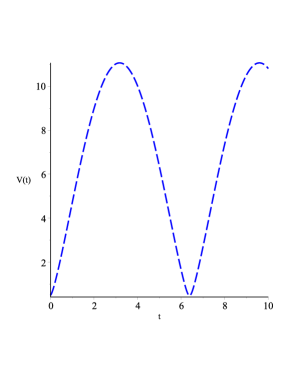
Figure 2: Evolution of the Universe filled with massive spinor field for a negative $\lambda_{2}$. In this case we set $\lambda_{1}=-1$ and $\lambda_{2}=-1$

.

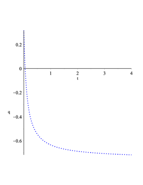
Figure 3: Plot of deceleration parameter $q$ for a positive $\lambda_{2}$. This case corresponds the evolution of volume scale given in Fig. 1

.

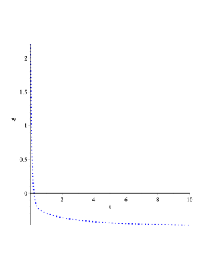
Figure 4: Evolution of EoS parameter $w$ for a positive $\lambda_{2}$. This case corresponds the evolution of volume scale given in Fig. 1

.

IV Conclusion

Within the scope of Bianchi type-III spacetime we study the role of spinor field on the evolution of the Universe. Unlike Bianchi type I, V or $VI_{0}$ cases where either both spinor mass and spinor field nonlinearity vanish sahaIJTP2014 ; sahaAPSS2015 ; sahabvi0 or the metric functions are similar to each other, i.e., $a_{1}\sim a_{2}\sim a_{3}$ in this case no such problem occurs. As one can see from (55) the spacetime remains locally rotationally symmetric and anisotropic all the time, though the isotropy of the spacetime can be achieved for a large proportionality constant. As far as evolution is concerned, depending on the sign of coupling constant the models allows both accelerated and oscillatory mode of expansion. A negative coupling constat leads to an oscillatory mode of expansion whereas a positive coupling constants generates expanding Universe with late time acceleration. Both deceleration parameter and EoS parameter in this case vary with time and are in agreement with modern concept of spacetime evolution.

Acknowledgments
This work is supported in part by a joint Romanian-LIT, JINR, Dubna Research Project 4338-6-14/16, theme no. 05-6-1119-2014/2016. Taking the opportunity I would also like to thank the reviewers for some helpful discussions and references.

References

- (1) A G Riess et al., Astron. J. 116, 1009 (1998)
- (2) S Perlmutter et al., Astrophys. J. 517, 565 (1999)
- (3) V Sahni and A A Starobinsky Int. J. Mod. Phys. D 9 373 (2000)
- (4) T Padmanabhan Phys. Rep. 380 235 (2003)
- (5) B Saha Astrophys. Space Sci. 302 83 (2006) DOI: 10.1007/s10509-005-9008-5
- (6) R Cardenas, T Gonzalez, Y Leiva, O Martin and I Quiros Phys. Rev. D 67 083501 (2003)
- (7) L P Chimento, A S Jakubi, D Pavon and W Zimdahl Phys. Rev. D 67 083513 (2003)
- (8) E V Linder General Relat. Grav. 40 329 (2008)
- (9) G Olivares, F Atrio-Barandela and D Pavon Phys. Rev. D 71 063523 (2005)
- (10) I Zlatev, L Wang and P J Steinhardt Phys. Rev. Lett. 82 896 (1999)
- (11) B Saha Chinese J. of Phys. 43 1035 (2005)
- (12) V Gorini, A Kamenshchik and U Moschella Phys. Rev. D 67 063509 (2003)
- (13) L Amendola, F Finelli, C Burigana and D Carturan J. Cosmology Astropart. Phys. 0307 005 (2003)
- (14) R Bean and O Dore Phys. Rev. D 68 023515 (2003)
- (15) M C Bento, O Bertolami and A A Sen Phys. Rev. D 66 043507 (2002)
- (16) M C Bento, O Bertolami and A A Sen Phys. Rev. D 67 063003 (2003)
- (17) M C Bento, O Bertolami and A A Sen Phys. Lett. B 575 172 (2003)
- (18) M Biesiada, W Godlowski and M Szydlowski Astrophys. J. 622 28 (2005)
- (19) N Bilic, G B Tupper and R D Viollier Phys. Lett. 353 17 (2002)
- (20) M Henneaux Phys. Rev. D 21, 857 (1980)
- (21) U Ochs and M Sorg Int. J. Theor. Phys. 32, 1531 (1993)
- (22) B Saha and G N Shikin Gen. Relat. Grav. 29, 1099 (1997)
- (23) B Saha and G N Shikin J Math. Phys. 38, 5305 (1997)
- (24) B Saha Phys. Rev. D 64, 123501 (2001)
- (25) C Armendriz-Picn and P B Greene Gen. Relat. Grav. 35, 1637 (2003)
- (26) B Saha and T Boyadjiev Phys. Rev. D 69, 124010 (2004)
- (27) B Saha Phys. Rev. D 69, 124006 (2004)
- (28) M O Ribas, F P Devecchi and G M Kremer Phys. Rev. D 72, 123502 (2005)
- (29) B Saha Phys. Particle. Nuclei. 37. Suppl. 1, S13 (2006)
- (30) B Saha Grav. Cosmol. 12(2-3)(46-47), 215 (2006)
- (31) B Saha Romanian Rep. Phys. 59, 649 (2007).
- (32) B Saha Phys. Rev. D 74, 124030 (2006)
- (33) R C de Souza and G M Kremer Class. Quantum Grav. 25, 225006 (2008)
- (34) G M Kremer and R.C de Souza arXiv:1301.5163v1 [gr-qc]
- (35) N J Popławski Phys. Lett. B 690, 73 (2010)
- (36) N J Popławski Phys. Rev. D 85, 107502 (2012)
- (37) N J Popławski Gen. Releat. Grav. 44, 1007 (2012)
- (38) L Fabbri Int. J. Theor. Phys. 52 634 (2013)
- (39) C W Misner Asrophys. J. 151, 431 (1968)
- (40) L Fabbri Phys. Rev. D 85 0475024 (2012)
- (41) S Vignolo, L Fabbri and R Cianci J. Math. Phys. 52 112502 (2011)
- (42) V G Krechet, M L Fel’chenkov and G N Shikin Grav. Cosmol. 14 No 3(55), 292 (2008)
- (43) B Saha Cent. Euro. J. Phys. 8, 920 (2010a)
- (44) B Saha Romanian Rep. Phys. 62, 209 (2010b)
- (45) B Saha Astrophys. Space Sci. 331, 243 (2011)
- (46) B Saha Int. J. Theor. Phys. 51, 1812 (2012)
- (47) B Saha Int. J. Theor. Phys. 53 1109 (2014) DOI: 10.1007/s10773-013-1906-7
- (48) B Saha Astrophys. Space Sci. 357 28 (2015) DOI 10.1007/s10509-015-2291-x
- (49) B Saha The European Physical Journal Plus 130 208 - 13 (2015) DOI 10.1140/epjp/i2015-15208-0
- (50) A A Coley and S Hervic Class. Quantum Grav. 25) 198001 (2008)
- (51) M K Yadav, A Rai and A Pradhan Int. J. Theor. Phys. 46 2677 (2007)
- (52) A Pradhan, H Amirhashchi and H Zainuddin Astrophys. Space Sci. 331 679 (2011)
- (53) A Pradhan, S Lata and H Amirhashchi Commun. Theor. Phys. 54 950 (2010)
- (54) A K Yadav and L Yadav Int. J. Theor. Phys. 50 218 (2011)
- (55) B Saha Int. J. Theor. Phys. 51 1812 (2012)DOI 10.1007/s10773-011-1059-5
- (56) B Saha B Phys. Part. Nucl. 45 issue 2, 349 (2014) DOI:10.1134/S1063779614020026
- (57) A Pradhan and B Saha Phys. Part. Nucl. 46(3) 310 (2015) DOI: 10.1134/S1063779615030028
- (58) O Akarsu and C B Kilinc Gen. Relat. Grav. bf 42 763 (2010)
- (59) K S Adhav, M R Ugale, C B Kale and M P Bhende Bulg. J. Phys. 34 260 (2007)
- (60) T W B Kibble J. Math. Phys. 2 212 (1961)
- (61) K S Thorne The Astrophys. J. 148 51 (1967)
- (62) R Kantowski and R K Sachs J. Math. Phys. 7 443 (1966)
- (63) J Kristian and R K Sachs Astrophys. J. 143 379 (1966)
- (64) C B Collins, E N Glass and D A Wilkinson Gen. Rel. Grav. 12 805 (1980)