Entropy production from chaoticity in Yang-Mills field theory with use of the Husimi function

Abstract

We investigate possible entropy production in Yang-Mills (YM) field theory by using a quantum distribution function called Husimi function $f_{\rm H}(A,E,t)$ for YM field, which is given by a coarse graining of Wigner function and non-negative. We calculate the Husimi-Wehrl (HW) entropy $S_{\rm HW}(t)=-{\rm Tr}f_{H}\log f_{H}$ defined as an integral over the phase-space, for which two adaptations of the test-particle method are used combined with Monte-Carlo method. We utilize the semiclassical approximation to obtain the time evolution of the distribution functions of the YM field, which is known to show a chaotic behavior in the classical limit. We also make a simplification of the multi-dimensional phase-space integrals by making a product ansatz for the Husimi function, which is found to give a 10-20 per cent over estimate of the HW entropy for a quantum system with a few degrees of freedom. We show that the quantum YM theory does exhibit the entropy production, and that the entropy production rate agrees with the sum of positive Lyapunov exponents or the Kolmogorov-Sinai entropy, suggesting that the chaoticity of the classical YM field causes the entropy production in the quantum YM theory.

Introduction.— Thermalization or entropy production in an isolated quantum system is a long-standing problem. The entropy of a quantum system may be given by von Neumann entropy $S_{\rm vN}=-\text{Tr}\,\rho\log\rho$ with $\rho$ being the density matrix vonNeumann , and taking into account that the time evolution of the quantum system is described by a unitary transformation $U(t)={\rm e}^{-iHt/\hbar}$, von Neumann entropy $S_{\rm vN}$ is shown to remain unchanged in time, which is an absurd consequence in contradiction to the reality. One possible way to avoid this puzzle is to assume that there is no isolated quantum system because any quantum system is surrounded by the environment composed of quantum fields described by, say, QED; the partial trace with respect to the environment would lead to a density matrix of a mixed state due to the entanglementZurek1991vd . For thermalization of a macroscopic quantum system, the old idea of von Neumann has been recently rediscovered, and then a lot of related works and developments are being made vonNeumann1929 ; Goldstein2010 ; see Tasaki2015 and references cited therein. It might be worth mentioning that the entanglement entropy of a quantum system may have a geometrical interpretation as is clearly shown by Ryu-Takayanagi’s formula Ryu:2006bv .

In this work, we do not intend to develop a master theory to describe thermalization or entropy production of a generic quantum system. Instead, we concentrate on entropy production in quantum systems whose classical counter parts are chaotic, and the semiclassical approximation is valid. There are many physical systems satisfying these characteristics CGC : Among them, we have in mind the problem of the early thermaliztion in high-energy heavy-ion collisions (see review Heinz02 and recent studies Baier01 ; Romatschke06 ; Muller06 ; Berges08 ; Iwazaki08 ; Fujii08 ; Fries08 ; Fries09 ; Fujii09 ; Kunihiro10 ; Fukushima12 ; Epelbaum13 ; Iida13 ; Iida14 ; Tsutsui15-1 ; Tsutsui15-2 ; Ruggieri15-1 ; Ruggieri15-2 ) at the relativistic heavy-ion collider in the Brookhaven National Laboratory WPBRAHMS ; WPPHENIX ; WPPHOBOS ; WPSTAR and the large hadron collider at CERN Muller12 .

Chaotic classical systems are characterized by the sensitive dependence of the trajectory on the initial condition, and trajectories starting from adjacent initial conditions with the difference $\delta X(0)$ in the phase space deviate exponentially $|\delta X(t)|=\exp(\lambda t)|\delta X(0)|$ from each other: The exponent $\lambda$ is called a Lyapunov exponent. Then one can readily imagine that the chaotic behavior makes the phase-space distribution $f(q,p)$ so complicated to generate a finite amount of entropy via a coarse graining in the classical Hamiltonian system. In this respect, it is interesting that the sum of positive Lyapunov exponents coincides with the Kolomogorov-Sinai entropy (see references in Ref. KSentropy ) or the production rate of entropy Pesin . Indeed, these have been demonstrated for a discrete classical system Latora1999 , where an explicit calculation of the Boltzmann-like entropy $S_{\text{B}}=-\text{Tr}f\log{f}$ was made with the distribution function $f(q,\,p)$ as obtained by a coarse graining of the phase space of the discrete system.

A natural extension of the above interesting work to a quantum system might be done with the application of the quantum mechanical distribution function, i.e., Wigner function $f_{W}(q,\,p)$ derived as a Weyl transform of the density matrix $\rho$ Wigner . However, since $f_{W}$ is a mere Weyl transform of $\rho$, it can not describe an entropy production of a pure quantum system, even apart from the fact that $f_{W}$ is not positive definite.

To circumvent this well known difficulty, let us recall that one can not distinguish two phase space points in a unit cell in quantum mechanics, and smearing in the phase space volume of $(2\pi\hbar)^{D}$ may be allowed, where $D$ is the degrees of freedom (DOF) of the system. As such a smeared distribution function, we adopt Husimi function $f_{\rm H}$ Husimi , which is obtained by a Gaussian smearing of Wigner function and semi-positive definite. Then, we can define the Boltzmann-like entropy in terms of $f_{\rm H}$ as $S_{\text{HW}}=-\text{Tr}\,f_{\rm H}\log{f_{\rm H}}$, where Tr means the integral over the phase space. This entropy was first introduced and called the classical entropy by Wehrl Wehrl1978 , and we call it Husimi-Wehrl (HW) entropy KMOS ; Tsukiji2015 . In the previous work Tsukiji2015 , the present authors examine thermalization of isolated quantum systems by using the HW entropy evaluated in the semiclassical approximation. It was shown that the semiclassical treatment works well in describing the entropy-production process of a couple of quantum mechanical systems whose classical counter systems are known to be chaotic. Two novel methods were also proposed to evaluate the time evolution of the HW entropy, the test-particle method and the two-step Monte-Carlo method, and it was demonstrated that the simultaneous application of the two methods ensures the reliability of the results of the HW entropy at a given time.

In this article, we extend the previous work Tsukiji2015 to the Yang-Mills (YM) field, which is known to be chaotic and has macroscopic number of positive Lyapunov exponents Kunihiro10 . We investigate the possible entropy production by constructing the Husimi function and calculating the HW entropy of the YM field in the semiclassical approximation. The initial condition we adopt for the equation of motion (EOM) of the YM field is motivated by the early stage of relativistic heavy ion collisions CGC ; Glasma .

There is, however, a caveat against this simple prescription that works for quantum mechanical systems with a few degrees of freedom because of the large number of the degrees of freedom peculiar to the field theory. Thus we also take a simple ansatz for the Husimi function, where we construct it by a product of Husimi function for each degree of freedom, although the classical EOM itself is solved numerically with the fully included nonlinear couplings. When applied to a quantum mechanical system with two-degrees of freedom, the ansatz gives 10 to 20 per-cent over estimate of the HW entropy. We also develop a novel efficient numerical method for calculating the HW entropy, which is a modification of the test-particle method. We show that the YM theory does exhibit the entropy production, and find that the entropy production rate agrees with the sum of positive Lyapunov exponents or KS entropy. As long as we know, this is the first work to calculate the time dependence of entropy in non-integrable field theory except for the kinetic entropy shown in Ref. Nishiyama .

Husimi-Wehrl entropy on the lattice.— We consider the $\text{SU}(N_{c})$ YM field on a $L^{3}$ lattice. In the temporal gauge, Hamiltonian in non-compact formalism is given by

$$H=\frac{1}{2}\sum_{x,a,i}E^{a}_{i}(x)^{2}+\frac{1}{4}\sum_{x,a,i,j}F^{a}_{ij}(x)^{2},$$ (1)

with $F^{a}_{ij}=\partial_{i}A^{a}_{j}(x)-\partial_{j}A^{a}_{i}(x)+\sum_{b,c}f^{abc}A^{b}_{i}(x)A^{c}_{j}(x)$. $N_{D}=3L^{3}(N_{c}^{2}-1)$ is the total DOF. We take the dimensionless gauge field $A$ and conjugate momentum $E$ normalized by the lattice spacing $a$ throughout this article. The coupling constant $g$ is also included in the definition of $A$ and $E$.

The Husimi-Wehrl entropy of the YM field is obtained as a natural extension of that in quantum mechanics by regarding $(A(x),E(x))$ as canonical variables. First, we define the Wigner function (referred to as the Wigner functional Mrowczynski1994 ) in terms of $A(x)$ and $E(x)$,

$$f_{\scriptscriptstyle{W}}[A,E;t]= \int\frac{DA^{\prime}}{(2\pi\hbar)^{N_{D}}}e^{i{E\cdot A^{\prime}}/{\hbar}}$$

$$\times\left\langle A+{A^{\prime}}/{2}\mid\hat{\rho}(t)\mid{A-A^{\prime}/2}\right\rangle.$$ (2)

where $A\cdot E=\sum_{i,a,x}A^{a}_{i}(x)E^{a}_{i}(x)$ is the inner product. The time evolution of the Wigner function is derived from the von Neumann equation,

$$\frac{\partial}{\partial t}f_{\scriptscriptstyle{W}}[A,E;t]=\frac{\partial H}{\partial A}\cdot\frac{\partial f_{\scriptscriptstyle{W}}}{\partial E}-\frac{\partial H}{\partial E}\cdot\frac{\partial f_{\scriptscriptstyle{W}}}{\partial A}+\mathcal{O}(\hbar^{2}).$$ (3)

In the semi-classical approximation, we ignore $\mathcal{O}(\hbar^{2})$ terms, then $f_{\scriptscriptstyle{W}}$ is found to be constant along the trajectory satisfying the classical equation of motion (EOM) (good review Ref. Polkovnikov10 ),

$$\dot{E}=-\frac{\partial H}{\partial A},\,\dot{A}=\frac{\partial H}{\partial E}.$$ (4)

Secondly, we introduce the Husimi function as the smeared Wigner function with the minimal Gaussian packet,

$$f_{\scriptscriptstyle{H}}[A,E;t]=\int\frac{DA^{\prime}DE^{\prime}}{(\pi\hbar)^{N_{D}}}\mathrm{e}^{-\Delta(A-A^{\prime})^{2}/\hbar-(E-E^{\prime})^{2}/\Delta\hbar}$$

$$\times f_{\scriptscriptstyle{W}}[A^{\prime},E^{\prime};t]\ ,$$ (5)

where $\Delta$ is the parameter for the range of Gaussian smearing. As in quantum mechanics, Husimi function is semi-positive definite;$f_{H}[A,E;t]\geq 0$, and we define the Husimi-Wehrl entropy as the Boltzmann’s entropy or the Wehrl’s classical entropy Wehrl1978 by adopting the Husimi function for the phase space distribution,

$${S_{\mathrm{HW}}}(t)=-\int\frac{DADE}{(2\pi\hbar)^{N_{D}}}f_{\scriptscriptstyle{H}}[A,E;t]\log f_{\scriptscriptstyle{H}}[A,E;t].$$ (6)

Numerical methods.— We calculate the time evolution of the HW entropy by two methods; test particle (TP) method and parallel test particle (pTP) method. The TP method is developed in Ref. Tsukiji2015 . The pTP method, an alternative method for two-step Monte Carlo method, requires less numerical cost and gives almost the same results as two-step Monte Carlo method. We have demonstrated that the HW entropy in some quantum mechanical systems are successfully obtained in these two methods, which are reviewed in the following.

In the test-particle method (TP), we assume that the Wigner function is a sum of the delta functions,

$$f_{\scriptscriptstyle{W}}[A,E;t]= \frac{(2\pi\hbar)^{N_{\mathrm{D}}}}{N_{\mathrm{TP}}}\sum_{i=1}^{N_{\mathrm{TP}}}\delta^{N_{\mathrm{D}}}(A-A_{i}(t))\,\delta^{N_{\mathrm{D}}}(E-E_{i}(t)),$$ (7)

where $N_{\rm TP}$ is the total number of the test particles. The initial conditions of the test particles are $(A_{i}(0),\,E_{i}(0))$  $(i=1,\,2,\dots,\,{N_{\mathrm{TP}}})$, which are chosen so as to well sample $f_{\scriptscriptstyle{W}}[A,E,0]$. The time evolution of the coordinates $(A_{i}(t),E_{i}(t))$ is determined so that it reproduces the EOM for $f_{\scriptscriptstyle{W}}[A,E,t]$, which is reduced to the canonical equation of motion Eq. (4) in the semiclassical approximation.

With the test-particle representation of the Wigner function, Eq. (7), the Husimi function is readily expressed as

$$f_{\scriptscriptstyle{H}}[A,E;t]= \frac{2^{N_{\mathrm{D}}}}{{N_{\mathrm{TP}}}}\sum_{i=1}^{{N_{\mathrm{TP}}}}e^{-\Delta(A-A_{i}(t))^{2}/\hbar-(E-E_{i}(t))^{2}/\Delta\hbar}\ .$$ (8)

It is noteworthy that the Husimi function here is a smooth function in contrast to the corresponding Wigner function in Eq. (7).

Substituting the Wigner function (8) into Eq. (6), the HW entropy in the test-particle method is finally given as,

$$S_{\mathrm{HW}}^{\mathrm{(TP,TTP)}}= -\frac{1}{{N_{\mathrm{TP}}}}\sum_{i=1}^{N_{\mathrm{TP}}}\int\frac{DADE}{(\pi\hbar)^{N_{\mathrm{D}}}}\,e^{-\Delta(A-A_{i}(t))^{2}/\hbar-(E-E_{i}(t))^{2}/\Delta\hbar}\log\left[\frac{2^{N_{\mathrm{D}}}}{{N_{\mathrm{TP}}}}\sum_{j=1}^{{N_{\mathrm{TP}}}}e^{-\Delta(A-A_{j}(t))^{2}/\hbar-(E-E_{j}(t))^{2}/\Delta\hbar}\right]$$

$$\simeq -\frac{1}{{N_{\mathrm{MC}}}{N_{\mathrm{TP}}}}\sum_{k=1}^{N_{\mathrm{MC}}}\sum_{i=1}^{N_{\mathrm{TP}}}\log\left[\frac{2^{N_{\mathrm{D}}}}{{N_{\mathrm{TP}}}}\sum_{j=1}^{{N_{\mathrm{TP}}}}e^{-\Delta(\bar{A}_{k}+A_{i}(t)-A_{j}(t))^{2}/\hbar-(\bar{E}_{k}+E_{i}(t)-E_{j}(t))^{2}/\Delta\hbar}\right].$$ (9)

Note here that the integral over $(A,E)_{i}$ for each $i$ has a support only around the positions of the test particles $(A_{i}(t),\,E_{i}(t))$ due to the Gaussian function, and we can effectively perform the Monte-Carlo integration in the second line. With a set of random numbers $(\bar{A},\bar{E})_{i}$ with standard deviations of $\sqrt{\hbar/2\Delta}$ and $\sqrt{\hbar\Delta/2}$, Monte-Carlo sampling point $(A,E)_{i}$ for each $i$ is generated as $(A,E)_{i}=(A_{i},E_{i})+(\bar{A},\bar{E})_{i}$. Total sample number of $(\bar{A},\bar{E})_{i}$ is denoted by ${N_{\mathrm{MC}}}$ throughout this letter.

In the parallel test particle method, we make test particles in and out of logarithm independent, while they are same samples in TP. Figure 1 shows the numerical results of the HW entropy in the two dimensional quantum mechanical system, whose Hamiltonian is given by

$$H=\frac{p^{2}_{1}}{2}+\frac{p^{2}_{2}}{2}+\frac{1}{2}q^{2}_{1}q^{2}_{2}+\frac{\epsilon}{4}q^{4}_{1}+\frac{\epsilon}{4}q^{4}_{2}.$$ (10)

This system is called a modified quantum Yang-Mills (mqYM) model in Ref. Tsukiji2015 . With increasing test-particle number, the HW entropy is found to converge from below (above) in the TP (pTP) method, then it is possible to give upper and lower limits of the entropy and to guess the converged value by comparing the results in the two methods.

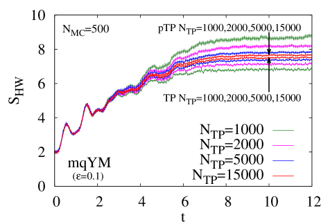
Figure 1: Time evolution of Husimi-Wehrl entropy for the modified quantum Yang-Mills mechanics in TP and pTP methods.

Product ansatz and example in a 2-dim quantum mechanical system.— While the extension to the field theory on the lattice is straightforward, the DOF are so large and numerical-cost demanding in quantum field theories that we need to invoke some approximation scheme in practical calculations. We here adopt product ansatz to avoid this difficulty.

In the ansatz, we construct the Husimi function as a product of that for one degree of freedom,

$$f_{\scriptscriptstyle{H}}^{\mathrm{(PA)}}[A,E;t]=\prod^{N_{D}}_{i}f_{\scriptscriptstyle{H}}^{(i)}(A_{i},E_{i};t)\ ,$$ (11)

where $f_{\scriptscriptstyle{H}}^{(i)}=\int\prod_{j\not=i}dA_{j}dE_{j}/2\pi\hbar\,f_{\scriptscriptstyle{H}}[A,E;t]$. By substituting this ansatz into Eq. (6), we obtain the HW entropy as a sum of the HW entropy for one degree of freedom;

$${S_{\mathrm{HW}}^{\mathrm{(PA)}}}=-\sum^{N_{D}}_{i=1}\int\frac{dA_{i}dE_{i}}{2\pi\hbar}f_{\scriptscriptstyle{H}}^{(i)}\,\log f_{\scriptscriptstyle{H}}^{(i)}\ .$$ (12)

The entropy estimated with the product ansatz gives the upper bound of the entropy, since it holds subadditivity. The subadditivity of entropy is expressed as

$$S_{1}(\rho_{1})+S_{2}(\rho_{2})\geq S_{12}(\rho_{12})\ ,$$ (13)

where $\rho_{1}=\int d\Gamma_{2}\rho_{12}$ and $\rho_{2}=\int d\Gamma_{1}\rho_{12}$ and $S_{1}$ and $S_{2}$ are subsystem entropies. In this paper, we apply it to the Husimi function and the Husimi-Wehrl entropy. Thus obtained entropy $S_{\mathrm{HW}}^{\mathrm{(PA)}}$ gives the upper bound of $S_{\mathrm{HW}}$ due to the subadditivity;

$$S_{\mathrm{HW}}\equiv S_{12...N_{D}}(\rho_{12...N_{D}}) \leq S_{1}(\rho_{1})+S_{23...N_{D}}(\rho_{23...N_{D}})$$

$$\leq\sum^{N_{D}}_{n}S_{n}(\rho_{n})=S_{\mathrm{HW}}^{\mathrm{(PA)}}\ .$$ (14)

To check the variety we apply it to the mqYM model previously discussed. Figure 2 shows the numerical results of the HW entropy with the product ansatz (${S_{\mathrm{HW}}^{\mathrm{(PA)}}}$) as well as the full entropy (${S_{\mathrm{HW}}}$), which can be found in Fig. 1. While ${S_{\mathrm{HW}}^{\mathrm{(PA)}}}$ slightly overestimates ${S_{\mathrm{HW}}}$, the difference is small enough to confirm entropy production. The HW entropy with product ansatz is found to agree with that without the ansatz within 10-20% error in a few dimensional quantum mechanical system. We also find that numerical results with the ansatz converge with smaller Monte Carlo samples, then it is much more efficient from the view point of numerical-cost reduction.

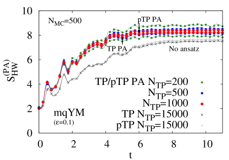
Figure 2: The variation in the product ansatz in the two-dimensional quantum model with TP and pTP methods. The green circle, blue square and orange triangle lines are the time evolution of HW entropy with the product ansatz in TP and pTP methods where the numbers of test-particles are ${N_{\mathrm{TP}}}=200,500$ and $1000$, respectively. The gray cross and black x lines are the time evolution of the HW entropy in both methods without the product ansatz ${N_{\mathrm{TP}}}=15000$.

Entropy production in Yang-Mills field theory.— We apply the above-mentioned framework to the SU(2) Yang-Mills field theory. The initial condition of the Winger function is set to be a Gaussian distribution, $f_{\scriptscriptstyle{W}}[A,E;t=0]=2^{N_{D}}\exp(-\omega{A}^{2}/\hbar-E^{2}/\omega\hbar)$, which corresponds to a coherent state. The Wigner-function evolution is obtained by solving the classical EOM, and the HW entropy with the product ansatz is calculated by using the TP and pTP methods. We take the parameter set, $\hbar=\omega=\Delta=1$.

In Fig. 3, we show the time evolution of the Husimi-Wehrl entropy per DOF with the product ansatz in TP and pTP methods. We find that the HW entropy per DOF is independent of the lattice size, and the extensive nature of entropy is confirmed. The dependence on the number of test-particle number is the same as that in quantum mechanics; With increasing Monte Carlo samples, ${S_{\mathrm{HW}}^{\mathrm{(PA)}}}$ converges from below and above in the TP and pTP methods, respectively. The results in the TP and pTP methods approach each other with increasing $N_{\rm TP}$ and we can guess that the converged value lies between these curves. After the oscillation around lattice time$=0.5$, the HW entropy increases in a monotonic way and its growth rate decreases. This means that the collective motion in the earliest stage damps, and the system approaches the equilibrium. The entropy saturation occurs at $t\sim 3$ in the lattice unit in the present setup.

The straight lines in Fig. 3 show the Kolmogorov-Sinai entropy rate, which is given in Ref. Kunihiro10 . The upper and lower lines show the sum of positive local and intermediate Lyapunov exponents (LLE and ILE), respectively. LLE are obtained as the eigen values of the second derivative matrix of the Hamiltonian, and ILE show the exponential growth rate in some time duration. Since the classical YM fields are conformal, the KS entropy rate should be proportional to $\varepsilon^{1/4}$ where $\varepsilon$ is the energy per site. The coefficients are evaluated in Ref. Kunihiro10 as $R_{\mathrm{KS}}^{\mathrm{LLE}}/L^{3}\simeq 3\times\varepsilon^{1/4}$ and $R_{\mathrm{KS}}^{\mathrm{ILE}}/L^{3}\simeq 2\times\varepsilon^{1/4}$ for the sum of positive LLE and ILE (local and intermediate KS entropy rate), respectively. These findings show that the local KS entropy rate characterizes the growth rate of the HW entropy in the early time and the intermediate KS entropy rate agrees with the average entropy growth until the thermalization time.

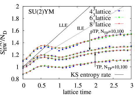
Figure 3: The time evolution of Husimi-Wehrl entropy for the SU(2) Yang-Mills field theory on $4^{3}$ lattice in TP and pTP methods with the product ansatz. The blue square, green circle and red triangle lines are the HW entropy per one degrees of freedom on $4^{3}$lattice, $6^{3}$lattice and $8^{3}$lattice, respectively. The black and gray solid lines show growth rates of LLE and ILE, respectively, given in Ref. Kunihiro10 .

Conclusion.— In summary, we have developed the numerical formulation to calculate the time evolution of the Husimi-Wehrl (HW) entropy in Yang-Mills field theory in the semi-classical approximation. This is a first work to calculate the time evolution of entropy in a non-integrable field theory except for the kinetic entropy shown in Ref. Nishiyama as long as we know. We have shown that the HW entropy is produced and the growth rates roughly agree with Lyapunov exponents. It should be noted that the time reversal invariance is kept in the present framework; in the time evolution of the Wigner function as well as in measuring the entropy. The produced entropy mainly comes from the complexity of the phase space distribution.

The entropy growth will have contribution to the thermalization process in relativistic heavy ion collisions. The set up in this article is motivated by the initial stage dynamics in relativistic heavy ion collisions. If we interpret the lattice spacing $a$ as the inverse saturation scale $Q_{s}^{-1}=0.2$ fm/c at RHIC, the lattice time scale is also normalized by the saturation scale $Q_{s}^{-1}$. This means that the observed entropy-saturation time ($t\sim 3$ in the lattice unit) is about $0.6$fm/c, which might be the encouraging result for the early thremalization scenario which is suggested by the hydrodynamical simulation (review Ref. Heinz02 ). For more realistic analysis, we should choose the initial condition such as the one given by the McLerran-Venugopalan model CGC .

References

- (1) J. von Neumann, Gött. Nach. 1927, 273 (1927); ”Mathematische Grundlagen der Quantenmechanik” (Springer, Berlin, 1932).
- (2) W. H. Zurek, Phys. Today 44N10, 36 (1991).
- (3) J. von Neumann, Z. Phys. 57, 30 (1929).
- (4) S. Goldstein, J.L. Lebowitz, R. Tumulka, N. Zanghi, J. H. 35, 173 (2010).
- (5) H. Tasaki, arXiv:1507.06479.
- (6) S. Ryu and T. Takayanagi, Phys. Rev. Lett. 96 181602 (2006).
- (7) U. Heinz and P. Kolb, Nucl. Phys. A702 269 (2002).
- (8) R. Baier, A.H. Mueller, D. Schiff, and D.T. Son, Phys. Lett. B 502, 51 (2001).
- (9) P. Romatschke and R. Venugopalan, Phys. Rev. Lett. 96, 062302 (2006).
- (10) B. Muller and A. Schafer, Phys. Rev. C 73, 054905 (2006).
- (11) J. Berges, S. Scheffler, and D. Sexty, Phys. Rev. D 77, 034504 (2008).
- (12) A. Iwazaki, Phys. Rev. C 77, 034907 (2008).
- (13) H. Fujii and K. Itakura, Nucl. Phys. A 809, 88 (2008).
- (14) R.J. Fries, B. Müller, and A. Schafer, Phys. Rev. C 78, 034913 (2008).
- (15) R.J. Fries, B. Muller, and A. Schafer, Phys. Rev. C 79, 034904 (2009).
- (16) H. Fujii, K. Itakura, and A. Iwasaki, Nucl. Phys. A 828, 178 (2009).
- (17) T. Kunihiro, B. Muller, A. Ohnishi, A. Schafer, T. T. Takahashi, and A. Yamamoto, Phys. Rev. D 88, 114015 (2010).
- (18) K. Fukushima and F. Gelis, Nucl. Phys. A 874, 108 (2012).
- (19) T. Epelbaum and F. Gelis, Phys. Rev. Lett. 111, 232301 (2013).
- (20) H. Iida, T. Kunihiro, B. Muller, A. Ohnishi, A. Schafer, and T.T. Takahashi, Phys. Rev. D 88, 094006 (2013).
- (21) H. Iida, T. Kunihiro, A. Ohnishi, and T. T. Takahashi, arXiv: 1410.7309.
- (22) S. Tsutsui, H. Iida, T. Kunihiro, and A. Ohnishi, Phys. Rev. D 91, 076003 (2015).
- (23) S. Tsutsui, T. Kunihiro, and A. Ohnishi, arXiv: 1512.00155.
- (24) M. Ruggieri, A. Puglisi, L. Oliva, S. Plumari, F. Scardina, and V. Greco, Phys. Rev. C 92, 064904 (2015).
- (25) M. Ruggieri, A. Puglisi, L. Oliva, S. Plumari, F. Scardina, V. Greco, arXiv: 1505.08081.
- (26) I. Arsenej, et al., Nucl. Phys. A 757, 1 (2005).
- (27) K. Adcox, et al., Nucl. Phys. A 757, 184 (2005).
- (28) B.B. Back, et al. Nucl. Phys. A 757, 28 (2005).
- (29) J. Adam, et al. Nucl. Phys. A 757, 102 (2005).
- (30) B. Muller, J. Schukraft, and B. Wyslouch, Annu. Rev. Nucl. Part. Sci. 62, 361 (2012).
- (31) A. J. Lichtenberg and M. A. Lieberman, “Regular and chaotic dynamics”, (Springer, New York, 1992).
- (32) Y. B. Pesin, Russian Math. Surveys, 55 (1977).
- (33) V. Latora and M. Baranger, Phys. Rev. Lett. 82, 520 (1999).
- (34) E.P. Wigner, Phys. Rev. 40, 749 (1932).
- (35) K. Husimi, Proc. Phys. Math. Soc. Jpn. 22, 123 (1940).
- (36) A. Wehrl, Rev. Mod. Phys. 50, 221 (1978).
- (37) T. Kunihiro, B. Muller, A. Ohnishi, and A. Schafer, Prog. Theor. Phys. 121, 555 (2009).
- (38) H. Tsukiji, H. Iida, T. Kunihiro, A. Ohnishi, and T. T. Takahashi, Prog. Theor. Exp. Phys. 083A01 (2015).
- (39) L.D. McLerran, and R. Venugopalan, Phys. Rev. D 49 2233 (1994); ibid. 49 3552 (1994): ibid. 50 2225 (1994).
- (40) T. Lappi and L. McLerran, Nucl. Phys. A772 220 (2006).
- (41) A. Nishiyama, Nucl. Phys. A 832, 289 (2010); A. Nishiyama and A. Ohnishi, Prog. Theor. Phys. 126, 249 (2011); Prog. Theor. Phys. 125, 775 (2011).
- (42) S. Mrowczynski and B. Muller, Phys. Rev. D 50, 7542 (1994).
- (43) A. Polkovnikov, arXiv: 0905.3384.