Stochastic quasi-Newton methods for non-strongly convex problems: convergence and rate analysis

Abstract

Motivated by applications in optimization and machine learning, we consider stochastic quasi-Newton (SQN) methods for solving stochastic optimization problems. In the literature, the convergence analysis of these algorithms relies on strong convexity of the objective function. To our knowledge, no theoretical analysis is provided for the rate statements in the absence of this assumption. Motivated by this gap, we allow the objective function to be merely convex and we develop a cyclic regularized SQN method where the gradient mapping and the Hessian approximation matrix are both regularized at each iteration and are updated in a cyclic manner. We show that, under suitable assumptions on the stepsize and regularization parameters, the objective function value converges to the optimal objective function of the original problem in both almost sure and the expected senses. For each case, a class of feasible sequences that guarantees the convergence is provided. Moreover, the rate of convergence in terms of the objective function value is derived. Our empirical analysis on a binary classification problem shows that the proposed scheme performs well compared to both classic regularization SQN schemes and stochastic approximation method.

I Introduction

In this paper, we study a stochastic optimization problem of the form:

$$\min_{x\in\mathbb{R}^{n}}f(x):=\mathsf{E}\!\left[F(x,\xi({\color[rgb]{0,0,0}\omega}))\right],$$ (1)

where $F:\mathbb{R}^{n}\times{\color[rgb]{0,0,0}\mathbb{R}^{d}}\to\mathbb{R}$ is a function, the random vector $\xi$ is defined as $\xi:\Omega\rightarrow\mathbb{R}^{d}$, $(\Omega,{\cal F},\mathbb{P})$ denotes the associated probability space and the expectation $\mathsf{E}\!\left[F(x,\xi)\right]$ is taken with respect to $\mathbb{P}$. A variety of applications can be cast as the model (1) (see [1, 2, 3, 4]). An important example in machine learning is the support vector machine (SVM) problem ([5, 6, 7]). In such problems, a training set containing a large number of input/output pairs $\{(u_{i},v_{i})\}_{i=1}^{N}\in\mathbb{R}^{m}\times\mathbb{R}$ is given where $v_{i}\in\{-1,1\}$ is the class’ index. The goal is to learn a classifier (e.g., a hyperplane) $h(x,u)$ where $x$ is the vector of parameters of the function $h$ and $u$ is the input data. To measure the distance of an observed output $v_{i}$ from the classifier function $h$, a real-valued convex loss function $\ell(h;v)$ is defined. The objective function is considered as the following averaged loss over the training set

$$f(x):=\frac{1}{N}\sum_{i=1}^{N}\ell(h(x,u_{i});v_{i}).$$ (2)

The preceding objective can be seen as a stochastic optimization model of the form (1), where $F(x,\xi):=\ell(h(x,u);v)$ and $\xi=(u,v)$.

Although, problem (1) may be seen as a deterministic problem, the challenges still arise when standard deterministic schemes are employed. In particular, when the expectation is over a general measure space (making computation of $\nabla_{x}\mathsf{E}\!\left[F(x,\xi)\right]$ difficult or impossible) or the distribution $\mathbb{P}$ is unavailable, standard gradient or Newton-based schemes cannot be directly applied. This has led to significant research on Monte-Carlo sampling techniques. Monte Carlo simulation methods have been used widely in the literature to solve stochastic optimization problems. Of these, sample average approximation (SAA) methods [8] and stochastic approximation (SA) methods ([9, 10]) (also referred to as stochastic gradient descent methods in the context of optimization) are among popular approaches. It has been discussed that when the sample size is large, the computational effort for implementing SAA schemes does not scale with the number of samples and these methods become inefficient ([10, 11]). SA methods, introduced by Robbins and Monro [9], require the construction of a sequence $\{x_{k}\}$, given a randomly generated $x_{0}\in\mathbb{R}^{n}$:

$$x_{k+1}:=x_{k}-\gamma_{k}\nabla{\color[rgb]{0,0,0}F}(x_{k},\xi_{k}),\quad\hbox{for }k\geq 0,$$ (SA)

where $\gamma_{k}>0$ denotes the stepsize and $\nabla F(x_{k},\xi_{k})$ denotes the sampled gradient of the function $f$ with respect to $x$ at $x_{k}$. Note that the gradient $\nabla F(x_{k},\xi_{k})$ is assumed to be an unbiased estimator of the true value of the gradient $\nabla f(x)$ at $x_{k}$, and assumed to be generated by a stochastic oracle. SA schemes are characterized by several disadvantages, including the poorer rate of convergence (than their deterministic counterparts) and the detrimental impact of conditioning on their performance. In deterministic regimes, when second derivatives are available, Newton schemes and their quasi-Newton counterparts have proved to be useful alternatives, particularly from the standpoint of displaying faster rates of convergence ([12, 13]).

Recently, there has been a growing interest in applying stochastic variants of quasi-Newton (SQN) methods for solving optimization and large scale machine learning problems. In these methods, $x_{k}$ is given by the following update rule:

$$x_{k+1}:=x_{k}-\gamma_{k}H_{k}^{-1}\nabla{\color[rgb]{0,0,0}F}(x_{k},\xi_{k}),\quad\hbox{for }k\geq 0,$$ (SQN)

where $H_{k}\succeq 0$ is an approximation of the Hessian matrix at iteration $k$ that incorporates the curvature information of the objective function within the algorithm. The convergence of this class of algorithms can be derived under a careful choice of the matrix $H_{k}$ and the stepsize sequence $\gamma_{k}$. In particular, boundedness of the eigenvalues of $H_{k}$ is an important factor in achieving global convergence in convex and nonconvex problems ([14, 15]). While in [16] the performance of SQN methods displayed to be favorable in solving high dimensional problems, Mokhtari et al. [17] developed a regularized BFGS method (RES) by updating the matrix $H_{k}$ according to a modified version of BFGS update rule to assure convergence. To address large scale applications, limited memory variants (L-BFGS) were employed to ascertain scalability in terms of the number of variables ([6, 18]). In a recent extension [19], a stochastic quasi-Newton method is presented for solving nonconvex stochastic optimization problems. Also, a variance reduced SQN method with a constant stepsize was developed [20] for smooth strongly convex problems characterized by a linear convergence rate.

Motivation: One of the main assumptions in the developed stochastic SQN method (e.g. [6, 18]) is the strong convexity of the objective function. Specifically, this assumption plays an important role in deriving the rate of convergence of the algorithm. However, in many applications, the objective function is convex, but not strongly convex such as, for example, the logistic regression function that is given by $\ell(u^{T}x,v):=\ln(1+\exp(-u^{T}xv))$ for $u,x\in\mathbb{R}^{n}$ and $v\in\mathbb{R}$. While lack of strong convexity might lead to a very slow convergence, no theoretical results on the convergence rate in given in the literature of stochastic SQN methods. A simple remedy to address this challenge is to regularize the objective function with the term $\frac{1}{2}\mu\|x\|^{2}$ and solve the approximate problem of the form

$$\min_{x\in\mathbb{R}^{n}}f(x)+\frac{\mu}{2}\|x\|^{2},$$ (3)

where $\mu>0$ is the regularization parameter. A trivial drawback of this technique is that the optimal solution to the approximate problem (3) is not an optimal of the original problem (3). Importantly, choosing $\mu$ to be a small number deteriorates the convergence rate of the algorithm. This issue is resolved in SA schemes through employing averaging techniques for non-strongly convex problems and they display the optimal rate of $\mathcal{O}\left(\frac{1}{\sqrt{k}}\right)$ (see [10, 21]). A limitation to averaging SA schemes is that boundedness of the gradient mapping is required to achieve such a rate.

Contributions: Motivated by these gaps, in this paper, we consider stochastic optimization problems with non-strongly convex objective functions and Lipschitz but possibly unbounded gradient mappings. We develop a so-called cyclic regularized stochastic BFGS algorithm to solve this class of problems. Our framework is general and can be adapted within other variants of SQN methods. Unlike the classic regularization, we allow the regularization parameter $\mu$, denoted by $\mu_{k}$, to be updated and decay to zero through implementing the iterations. This enables the generated sequence to approach to the optimal solution of the original problem and also, benefits the scheme by guaranteeing a derived rate of convergence. A challenge in employing this technique is to maintain the secant condition and ascertain the positive definiteness of the BFGS matrix. We overcome this difficulty by carefully updating the regularization parameter and the BFGS matrix in a cyclic manner. We show that, under suitable assumptions on the stepsize and the regularization parameter (referred to as tuning sequences), the objective function value converges to the exact optimal value in an almost sure sense. Moreover, we show that under different settings, the algorithm achieves convergence in mean and we derive and upper bound for the error of the algorithm in terms of the tuning sequences. We complete our analysis by showing that under a specific choice of the tuning sequences, the rate of convergence in terms of the objective function value is of the order $\frac{1}{\sqrt[5]{k}}$.

The rest of the paper is organized as follows. Section II presents the outline of the proposed algorithm addressing problems with non-strongly convex objectives. In Section III, we prove the convergence of the scheme in both almost sure and expected senses and derive the rate statement. We present the numerical experiments in Section IV. The paper ends with some concluding remarks in Section V.

Notation: A vector $x$ is assumed to be a column vector and $x^{T}$ denotes its transpose, while $\|x\|$ denotes the Euclidean vector norm, i.e., $\|x\|=\sqrt{x^{T}x}$. We write a.s. as the abbreviation for “almost surely”. For a symmetric matrix $B$, we write $\lambda_{min}(B)$ to denote its smallest eigenvalue. We use $\mathsf{E}\!\left[z\right]$ to denote the expectation of a random variable $z$. A function $f:X\subset\mathbb{R}^{n}\rightarrow\mathbb{R}$ is said to be strongly convex with parameter $\mu>0$, if $f(y)\geq f(x)+\nabla f(y)^{T}(y-x)+\frac{\mu}{2}\|x-y\|^{2},$ for any $x,y\in X$. A mapping $F:X\subset\mathbb{R}^{n}\rightarrow\mathbb{R}$ is Lipschitz continuous with parameter $L>0$ if for any $x,y\in X$, we have $\|F(x)-F(y)\|\leq L\|x-y\|$.

II Outline of the algorithm

We begin by stating our general assumptions for problem (1). The underlying assumption in this paper is that the function $f$ is convex and smooth.

Assumption 1

1. The function $F(x,\xi)$ is convex with respect to $x$ for any $\xi\in\Omega$.

2. $f(x)$ is continuously differentiable with Lipschitz continuous gradients over $\mathbb{R}^{n}$ with parameter $L>0$.

3. The optimal solution set of problem (1) is nonempty.

Next, we state the assumptions on the random variable $\xi$ and the properties of the stochastic estimator of the gradient mapping, i.e. $\nabla F$.

Assumption 2

1. Random variables $\xi_{k}$ are i.i.d. for any $k\geq 0$;

2. The stochastic gradient mapping $\nabla F(x,\xi)$ is an unbiased estimator of $\nabla f(x)$, i.e. $\mathsf{E}\!\left[\nabla F(x,\xi)\right]=\nabla f(x)$, and has bounded variance, i.e., there exists a scalar $\nu>0$ such that $\mathsf{E}\!\left[\|\nabla F(x,\xi)-\nabla f(x)\|^{2}\right]\leq\nu^{2}$ for any $x\in\mathbb{R}^{n}$.

To solve (1), we propose a regularization algorithm that generates a sequence $\{x_{k}\}$ for any $k\geq 0$:

$$x_{k+1}:=x_{k}-\gamma_{k}\left(B_{k}^{-1}+\delta_{k}\mathbf{I}\right)\left(\nabla F(x_{k},\xi_{k})+\mu_{k}x_{k}\right).$$ (CR-SQN)

Here, $\gamma_{k}>0$ denotes the stepsize at iteration $k$, $B_{k}$ denotes the approximation of the Hessian matrix, $\mu_{k}>0$ is the regularization parameter of the gradient mapping where

$$\begin{cases}\mu_{k+1}=\mu_{k},&\text{if }k\text{ is even}\\ \mu_{k+1}<\mu_{k},&\text{if }k\text{ is odd},\end{cases}$$ (4)

while $\delta_{k}>0$ is the regularization parameter of the matrix $H_{k}$. We assume when $k$ is even, $\mu_{k}<\mu_{k-1}$ is chosen such that $\nabla F(x_{k},\xi_{k})+\mu_{k}x_{k}\neq 0$. Let us define the matrix $B_{k}$ by the following rule:

$$B_{k+1}:=\begin{cases}B_{k}-\frac{B_{k}s_{k}{\color[rgb]{0,0,0}s_{k}^{T}}B_{k}}{s_{k}^{T}B_{k}s_{k}}+\frac{{y_{k}^{B}}(y_{k}^{B})^{T}}{s_{k}^{T}{y_{k}^{B}}}+\rho\mu_{k}\mathbf{I},&k\text{ even}\\ B_{k},&k\text{ odd},\end{cases}$$ (5)

where for an even $k$,

$$s_{k}:=x_{k+1}-x_{k},$$

$${y_{k}^{B}}:=\nabla F(x_{k+1},\xi_{k})-\nabla F(x_{k},\xi_{k})+(1-\rho)\mu_{k}s_{k},$$

and $0<\rho<1$ is the regularization factor of the matrix $B_{k+1}$ at iteration $k$. To state the properties of the matrix $B_{k}$, we start by defining the regularized function.

Definition 1

Consider the sequence $\{\mu_{k}\}$ of positive scalars. The regularized function $f_{k}:\mathbb{R}^{n}\to\mathbb{R}$ is defined as follows:

$$f_{k}(x):=f(x)+\frac{\mu_{k}}{2}{\|x\|^{2}},\quad\hbox{for any }k\geq 0.$$

Similar notation can be used for the regularized stochastic function $F_{k}$ as $F_{k}(x,\xi):=F(x,\xi)+\frac{\mu_{k}}{2}\|x\|^{2}$. We can now define the term $y^{reg}_{k}$ as the difference between the value of the regularized stochastic gradient mappings at two consecutive points as follows:

$$y^{reg}_{k}:=\nabla F_{k}(x_{k+1},\xi_{k})-\nabla F_{k}(x_{k},\xi_{k}).$$

In the following result, we show that at iterations that the matrix $B_{k}$ is updated, the secant condition is satisfied implying that $B_{k}$ is well-defined. Also, we show that $B_{k}$ is positive definite for $k\geq 0$.

Lemma 1

Let Assumption 1(a) hold, and let $B_{k}$ be given by the update rule (5). Suppose $B_{0}\succeq\rho\mu_{0}\mathbf{I}$ is a symmetric matrix. Then, for any even $k$, the secant condition holds, i.e., $s_{k}^{T}{y_{k}^{B}}>0$, and $B_{k+1}s_{k}={y}^{reg}_{k}$. Moreover, for any $k$, $B_{k}$ is symmetric and $B_{k+1}\succeq\rho\mu_{k}\mathbf{I}$.

Proof:

It can be easily seen, by the induction on $k$, that all $B_{k}$ are symmetric when $B_{0}$ is symmetric, assuming that the matrices are well defined. We use the induction on even values of $k$ to show that the other statements hold and that the matrices are well defined. Suppose $k\geq 2$ is even and for any even values of t with $t<k$, we have $s_{t}^{T}{y_{t}^{B}}>0$, $B_{t+1}s_{t}={y}^{reg}_{t}$, and $B_{t+1}\succeq\rho\mu_{t}\mathbf{I}$. We show that all of these relations hold for $t=k$, i.e., $s_{k}^{T}{y_{k}^{B}}>0$, $B_{k+1}s_{k}={y}^{reg}_{k}$, and $B_{k+1}\succeq\rho\mu_{k}\mathbf{I}$. First, we prove that the secant condition holds. We can write

$$s_{k}^{T}{y_{k}^{B}} =(x_{k+1}-x_{k})^{T}(\nabla F(x_{k+1},\xi_{k})-\nabla F(x_{k},\xi_{k})$$

$$\quad+(1-\rho)\mu_{k}(x_{k+1}-x_{k}))$$

$$\geq(1-\rho)\mu_{k}\|x_{k+1}-x_{k}\|,$$

where we used the convexity of $F(\cdot,\xi)$.

From the induction hypothesis, $B_{k-1}\succeq\rho\mu_{k-2}\textbf{I}$ since $k-2$ is even. Furthermore, since $k-1$ is odd, we have $B_{k}=B_{k-1}$ by the update rule (5). Therefore, $B_{k}$ is positive definite. Note that since $k$ is even, the choice of $\mu_{k}$ is such that $\nabla F(x_{k},\xi_{k})+\mu_{k}x_{k}\neq 0$ (see the discussion following (4)). Since $B_{k}$ is positive definite, the matrix $B_{k}^{-1}+\delta_{k}\mathbf{I}$ is positive definite. Therefore, we have $\left(B_{k}^{-1}+\delta_{k}\mathbf{I}\right)\left(\nabla F(x_{k},\xi_{k})+\mu_{k}x_{k}\right)\neq 0$, implying that $x_{k+1}\neq x_{k}$. Hence

$$s_{k}^{T}{y_{k}^{B}}\geq(1-\rho)\mu_{k}\|x_{k+1}-x_{k}\|^{2}>0,$$

where we used $\rho<1$. Thus, the secant condition holds.

Also, since $k-1$ is odd, by update rule (4), it follows that $\mu_{k}=\mu_{k-1}$. From the update rule (5) and that $B_{k}$ is positive definite and symmetric, we have

$$B_{k+1} \succeq B^{0.5}\left(\textbf{I}-\frac{B_{k}^{0.5}s_{k}(s_{k})^{T}B_{k}^{0.5}}{\|B_{k}^{0.5}s_{k}\|^{2}}\right)B^{0.5}+\rho\mu_{k}\mathbf{I},$$ (6)

where the last relation is due to ${y_{k}^{B}}(y_{k}^{B})^{T}\succeq 0$ and $s_{k}^{T}{y_{k}^{B}>}0$.

Since $x_{k+1}\neq x_{k}$ we have $s_{k}^{T}B_{k}s_{k}\neq 0$. Thus, the matrix $\textbf{I}-\frac{B_{k}^{0.5}s_{k}(s_{k})^{T}B_{k}^{0.5}}{\|s_{k}^{T}B_{k}^{0.5}\|^{2}}$ is well defined and positive semidefinite, since it is symmetric with eigenvalues are between 0 and 1.

Next, we show that $B_{k+1}$ satisfies $B_{k+1}s_{k}=y_{k}^{reg}$. Using the update rule (5), for even $k$ we have,

$$B_{k+1}s_{k} =B_{k}s_{k}{\color[rgb]{0,0,0}-\frac{B_{k}s_{k}s_{k}^{T}B_{k}s_{k}}{s_{k}^{T}B_{k}s_{k}}+\frac{y_{k}^{B}(y_{k}^{B})^{T}s_{k}}{s_{k}^{T}{y_{k}^{B}}}}+\rho\mu_{k}s_{k}$$

$$=B_{k}s_{k}{\color[rgb]{0,0,0}-B_{k}s_{k}+y_{k}^{B}}+\rho\mu_{k}s_{k}$$

$$=\nabla F(x_{k+1},\xi_{k})-\nabla F(x_{k},\xi_{k}){\color[rgb]{0,0,0}+\mu_{k}s_{k}}.$$

Since $k$ is even, we have $\mu_{k+1}=\mu_{k}$ implying that

$$B_{k+1}s_{k} =\nabla F(x_{k+1},\xi_{k})-\nabla F(x_{k},\xi_{k})$$

$$+\mu_{k+1}x_{k+1}-\mu_{k}x_{k}$$

$$=\nabla F_{k}(x_{k+1},\xi_{k})-\nabla F_{k}(x_{k},\xi_{k})=y_{k}^{reg},$$

where the last equality follows by the definition of the regularized mappings.

From the preceding discussion, we conclude that the induction hypothesis holds also for $t=k$. Therefore, all the desired results hold for any even $k$. To complete the proof, we need to show that for any odd $k$, we have $B_{k+1}=B_{k}\succeq\rho\mu_{k}\textbf{I}$. By the update rule (5), we have $B_{k+1}=B_{k}$. Since $k-1$ is even, $B_{k}\succeq\rho\mu_{k-1}\textbf{I}$. Also, from (4) we have $\mu_{k}=\mu_{k-1}$. Therefore, $B_{k+1}=B_{k}\succeq\rho\mu_{k}\textbf{I}$. ∎

III Convergence Analysis

In this section, we analyze the convergence properties of the stochastic recursion  (CR-SQN). The following assumption provides the required conditions on the stepsize sequence $\gamma_{k}$ and is a commonly used assumption in the regime of stochastic approximation methods [17, 19, 6].

Property 1

[Properties of the regularized function] The function $f_{k}$ from Definition 1 for any $k\geq 0$ has the following properties:

• $f_{k}$ is strongly convex with a parameter $\mu_{k}$.

• $f_{k}$ has Lipschitzian gradients with parameter $L+\mu_{k}$.

• $f_{k}$ has a unique minimizer over $\mathbb{R}^{n}$, denoted by $x^{*}_{k}$. Moreover, for any $x\in\mathbb{R}^{n}$,

  $$2\mu_{k}(f_{k}(x)-f_{k}(x^{*}_{k}))\leq\|\nabla f_{k}(x)\|^{2},$$

  $$\|\nabla f_{k}(x)\|^{2}\leq 2(L+\mu_{k})(f_{k}(x)-f_{k}(x^{*}_{k})).$$

The existence and uniqueness of $x^{*}_{k}$ in Property 1(c) is due to the strong convexity of the function $f_{k}$ (see, for example, Sec. 1.3.2 in [22]), while the relation for the gradient is known to hold for a strongly convex function with a parameter $\mu$ that also has Lipschitz gradients with a parameter $L$ (see Lemma 1 in page 23 in [22]).

The next result provides an important property for the recursion (CR-SQN) that will be subsequently used to show the convergence of the scheme. Throughout, we let $\mathcal{F}_{k}$ denote the history of the method up to time $k$, i.e., $\mathcal{F}_{k}=\{x_{0},\xi_{0},\xi_{1},\ldots,\xi_{k-1}\}$ for $k\geq 1$ and $\mathcal{F}_{0}=\{x_{0}\}$. Also, we denote the stochastic error of the regularized gradient estimator by

$$w_{k}:=\nabla F(x_{k},\xi_{k})-\nabla f(x_{k}),{\color[rgb]{0,0,0}\quad\hbox{for all }k\geq 0.}$$ (7)

Lemma 2

[A recursive error bound inequality] Consider the algorithm (CR-SQN). Suppose sequences $\gamma_{k}$, $\delta_{k}$, and $\mu_{k}$ are chosen such that for any $k\geq 0$, $\mu_{k}$ satisfies (4), and

$$(L+\mu_{k})^{2}\gamma_{k}\left((\rho\mu_{k-1})^{-1}+\delta_{k}\right)^{2}\leq\delta_{k}\mu_{k}.$$ (8)

Under Assumptions 1 and 2, for any $k\geq 1$ and any optimal solution $x^{*}$, we have

$$\mathsf{E}\!\left[f_{k+1}(x_{k+1})\mid\mathcal{F}_{k}\right]-f^{*}$$ (9)

$$\leq(1-\gamma_{k}\delta_{k}\mu_{k})\left(f_{k}(x_{k})-f^{*}\right)+\gamma_{k}\delta_{k}\frac{\mu_{k}^{2}}{2}\|x^{*}\|^{2}$$

$$+\frac{(L+\mu_{k})}{2}\gamma_{k}^{2}\left((\rho\mu_{k-1})^{-1}+\delta_{k}\right)^{2}\nu^{2}.$$ (10)

Proof:

The Lipschitzian property of $\nabla f_{k}$ (see Property 1(b)) and the recursion (CR-SQN) imply that

$$f_{k}(x_{k+1})\leq f_{k}(x_{k})+\nabla f_{k}(x_{k})^{T}(x_{k+1}-x_{k})$$

$$+\frac{(L+\mu_{k})}{2}\|x_{k+1}-x_{k}\|^{2}$$

$$=f_{k}(x_{k})-\gamma_{k}\nabla f_{k}(x_{k})^{T}\left(B_{k}^{-1}+\delta_{k}\mathbf{I}\right)(\nabla F(x_{k},\xi_{k})+\mu_{k}x_{k})$$

$$+\frac{(L+\mu_{k})}{2}\gamma_{k}^{2}\|\left(B_{k}^{-1}+\delta_{k}\mathbf{I}\right)(\nabla F(x_{k},\xi_{k})+\mu_{k}x_{k})\|^{2}.$$

From the definition of the stochastic error $w_{k}$ (see (7)) and and the definition of the regularized function (see Definition 1), we have

$$\nabla F(x_{k},\xi_{k})+\mu_{k}x_{k}=\nabla f(x_{k})+\mu_{k}x_{k}+w_{k}=\nabla f_{k}(x_{k})+w_{k}.$$

Hence,

$$f_{k}(x_{k+1})\leq f_{k}(x_{k})$$

$$\ -\gamma_{k}\nabla f_{k}(x_{k})^{T}(B_{k}^{-1}+\delta_{k}\mathbf{I})(\nabla f_{k}(x_{k})+w_{k})$$

$$\ +\frac{(L+\mu_{k})}{2}\gamma_{k}^{2}\|\left(B_{k}^{-1}+\delta_{k}\mathbf{I}\right)(\nabla f_{k}(x_{k})+w_{k})\|^{2}$$

$$\leq f_{k}(x_{k})-\gamma_{k}\lambda_{min}\left(B_{k}^{-1}+\delta_{k}\mathbf{I}\right)\|\nabla f_{k}(x_{k})\|^{2}$$

$$\ {\color[rgb]{0,0,0}-\gamma_{k}\nabla f_{k}(x_{k})^{T}\left(B_{k}^{-1}+\delta_{k}\mathbf{I}\right)w_{k}}$$

$$\ +{\color[rgb]{0,0,0}\frac{(L+\mu_{k})}{2}\gamma_{k}^{2}\|B_{k}^{-1}+\delta_{k}\mathbf{I}\|^{2}\left(\|\nabla f_{k}(x_{k})+w_{k}\|^{2}\right)}.$$

Note that Lemma 1(b) implies that

$$\delta_{k}\textbf{I}\preceq B_{k}^{-1}+\delta_{k}{\color[rgb]{0,0,0}\textbf{I}}\preceq\left((\rho\mu_{k-1})^{-1}+\delta_{k}\right)\textbf{I}.$$

From the preceding two relations we obtain

$$f_{k}(x_{k+1})\leq f_{k}(x_{k})-\gamma_{k}\delta_{k}\|\nabla f_{k}(x_{k})\|^{2}$$

$$\ -\gamma_{k}\nabla f_{k}(x_{k})^{T}\left(B_{k}^{-1}+\delta_{k}\mathbf{I}\right)w_{k}$$

$$+\frac{(L+\mu_{k})}{2}\gamma_{k}^{2}\left((\rho\mu_{k-1})^{-1}+\delta_{k}\right)^{2}\|\nabla f_{k}(x_{k})+w_{k}\|^{2}.$$

Next, we take the expected value from both sides with respect to $\mathcal{F}_{k}$. Note that the matrix $B_{k}$ and $x_{k}$ are both deterministic parameters if the history $\mathcal{F}_{k}$ is known. Note that from Assumption 2, $\mathsf{E}\!\left[w_{k}\mid\mathcal{F}_{k}\right]=0$ and $\mathsf{E}\!\left[\|w_{k}\|^{2}\mid\mathcal{F}\right]\leq\nu^{2}$. Therefore,

$$\mathsf{E}\!\left[\|\nabla f_{k}(x_{k})+w_{k}\|^{2}\mid\mathcal{F}_{k}\right]\leq\|\nabla f_{k}(x_{k})\|^{2}+\nu^{2}.$$

Thus, we obtain

$$\mathsf{E}\!\left[f_{k}(x_{k+1})\mid\mathcal{F}_{k}\right]\leq f_{k}(x_{k})-\gamma_{k}\delta_{k}\|\nabla f_{k}(x_{k})\|^{2}$$

$$\ +\frac{(L+\mu_{k})}{2}\gamma_{k}^{2}\left((\rho\mu_{k-1})^{-1}+\delta_{k}\right)^{2}\left(\|\nabla f_{k}(x_{k})\|^{2}+\nu^{2}\right).$$

Using Property 1(c) for the function $f_{k}$, we have

$$\mathsf{E}\!\left[f_{k}(x_{k+1})\mid\mathcal{F}_{k}\right]\leq f_{k}(x_{k})-2\gamma_{k}\delta_{k}\mu_{k}\left(f_{k}(x_{k})-f_{k}(x_{k}^{*})\right)$$

$$\ +(L+\mu_{k})^{2}\gamma_{k}^{2}\left((\rho\mu_{k-1})^{-1}+\delta_{k}\right)^{2}\left(f_{k}(x_{k})-f_{k}(x_{k}^{*})\right)$$

$$\ +\frac{(L+\mu_{k})^{2}}{2}\gamma_{k}^{2}\left((\rho\mu_{k-1})^{-1}+\delta_{k}\right)^{2}\nu^{2}.$$

Due to our assumption on the choice of the sequences $\gamma_{k}$, $\delta_{k}$ and $\mu_{k}$, we have $(L+\mu_{k})^{2}\gamma_{k}^{2}\left((\rho\mu_{k-1})^{-1}+\delta_{k}\right)^{2}\leq\gamma_{k}\delta_{k}\mu_{k}$. Thus,

$$\mathsf{E}\!\left[f_{k}(x_{k+1})\mid\mathcal{F}_{k}\right]\leq f_{k}(x_{k})-\gamma_{k}\delta_{k}\mu_{k}\left(f_{k}(x_{k})-f_{k}(x^{*}_{k})\right)$$ (11)

$$+\frac{(L+\mu_{k})^{2}}{2}\gamma_{k}^{2}\left((\rho\mu_{k-1})^{-1}+\delta_{k}\right)^{2}\nu^{2}.$$ (12)

In the last step, we build a recursive inequality for the error term $f_{k}(x_{k})-f^{*}$. Adding and subtracting $f^{*}$, we obtain

$$f_{k}(x_{k})-f_{k}(x^{*}_{k})=\left(f_{k}(x_{k})-f^{*}\right)+\left(f^{*}-f_{k}(x^{*}_{k})\right)$$

$$=\left(f_{k}(x_{k})-f^{*}\right)+\left(f_{k}(x^{*})-\frac{\mu_{k}}{2}\|x^{*}\|^{2}-f_{k}(x^{*}_{k})\right),$$

where the last equality follows from $f^{*}=f_{k}(x^{*})-\frac{\mu_{k}}{2}\|x^{*}\|^{2}$. Since $x^{*}_{k}$ is the minimizer of $f_{k}(x^{*}_{k})$, we have $f_{k}(x^{*})-f_{k}(x^{*}_{k})\geq 0$, implying that

$$f_{k}(x_{k})-f_{k}(x^{*}_{k})\geq f_{k}(x_{k})-f^{*}-\frac{\mu_{k}}{2}\|x^{*}\|^{2}.$$

By substituting the preceding inequality in (11), we obtain

$$\mathsf{E}\!\left[f_{k}(x_{k+1})\mid\mathcal{F}_{k}\right]\leq f_{k}(x_{k})-\gamma_{k}\delta_{k}\mu_{k}\left(f_{k}(x_{k})-f^{*}\right)$$

$$+\gamma_{k}\delta_{k}{\color[rgb]{0,0,0}\frac{\mu_{k}^{2}}{2}}\|x^{*}\|^{2}+{\color[rgb]{0,0,0}\frac{(L+\mu_{k})}{2}}\gamma_{k}^{2}\left((\rho\mu_{k-1})^{-1}+\delta_{k}\right)^{2}\nu^{2}.$$

By subtracting $f^{*}$ from both sides of the preceding inequality, we see that

$$\mathsf{E}\!\left[f_{k}(x_{k+1})\mid\mathcal{F}_{k}\right]-f^{*}\leq\left(1-\gamma_{k}\delta_{k}\mu_{k}\right)\left(f_{k}(x_{k})-f^{*}\right)$$

$$+\gamma_{k}\delta_{k}\frac{\mu_{k}^{2}}{2}\|x^{*}\|^{2}+\frac{(L+\mu_{k})}{2}\gamma_{k}^{2}\left((\rho\mu_{k-1})^{-1}+\delta_{k}\right)^{2}\nu^{2}.$$

Next, we relate the values $f_{k+1}(x_{k+1})$ and $f_{k}(x_{k+1})$. From Definition 1 and $\mu_{k}$ being non-increasing we can write

$$f_{k+1}(x_{k+1}) =f(x_{k+1})+\frac{\mu_{k+1}}{2}\|x_{k+1}\|^{2}$$

$$\leq f(x_{k+1})+\frac{\mu_{k}}{2}\|x_{k+1}\|^{2}=f_{k}(x_{k+1}).$$

Therefore, the desired inequality (9) holds. ∎

We make use of the following result, which can be found in [22] (see Lemma 11 on page 50).

Lemma 3

Let $\{v_{k}\}$ be a sequence of nonnegative random variables, where $\mathsf{E}\!\left[v_{0}\right]<\infty$, and let $\{\alpha_{k}\}$ and $\{\beta_{k}\}$ be deterministic scalar sequences such that:

$$\mathsf{E}\!\left[v_{k+1}|v_{0},\ldots,v_{k}\right]\leq(1-\alpha_{k})v_{k}+\beta_{k}\quad a.s.\ \hbox{for all }k\geq 0,$$

$$0\leq\alpha_{k}\leq 1,\quad\ \beta_{k}\geq 0,$$

$$\quad\ \sum_{k=0}^{\infty}\alpha_{k}=\infty,\quad\ \sum_{k=0}^{\infty}\beta_{k}<\infty,\quad\ \lim_{k\to\infty}\,\frac{\beta_{k}}{\alpha_{k}}=0.$$

Then, $v_{k}\rightarrow 0$ almost surely.

In order to apply Lemma 3 to the inequality (9) and prove the almost sure convergence, we use the following definitions:

$$v_{k}:=f_{k}(x_{k})-f^{*},\quad\alpha_{k}:=\gamma_{k}\delta_{k}\mu_{k},$$

$$\beta_{k}:=\gamma_{k}\delta_{k}\mu_{k}^{2}\|x^{*}\|^{2}+(L+\mu_{k})\gamma_{k}^{2}\left((\rho\mu_{k-1})^{-1}+\delta_{k}\right)^{2}\nu^{2}.$$ (13)

To satisfy the conditions of Lemma 3, we identify a set of sufficient conditions on the sequences $\{\gamma_{k}\},\{\mu_{k}\}$, and $\{\delta_{k}\}$ in forthcoming assumption. Later in Lemma 4, we provide a class of sequences that meet these assumptions.

Assumption 3

[Sufficient conditions on sequences for a.s. convergence] Let the sequences $\{\gamma_{k}\},\{\mu_{k}\}$, and $\{\delta_{k}\}$ be non-negative and satisfy the following conditions:

• $\lim_{k\to\infty}\frac{\gamma_{k}}{\mu_{k}^{3}\delta_{k}}=0$;

• $\delta_{k}\mu_{k-1}\leq 1$ for $k\geq 1$;

• $\mu_{k}$ satisfies (4) and $\mu_{k}\to 0$;

• $\sum_{k=0}^{\infty}\gamma_{k}\delta_{k}\mu_{k}=\infty$;

• $\sum_{k=0}^{\infty}\left(\frac{\gamma_{k}}{\mu_{k}}\right)^{2}<\infty$;

• $\sum_{k=0}^{\infty}\gamma_{k}\delta_{k}\mu_{k}^{2}<\infty$;

• $\gamma_{k}\delta_{k}\mu_{k}\leq 1$ for $k\geq 0$;

With Assumption 3, we have the following result.

Theorem 1

[Almost sure convergence] Consider the algorithm (CR-SQN). Suppose Assumptions 1, 2 and 3 hold. Then, $\lim_{k\to\infty}f(x_{k})=f^{*}$ a.s.

Proof:

First, note that from Assumption 3(a), there exists $K\geq 1$ such that for any $k\geq K$ we have $\frac{4\gamma_{k}}{\rho^{2}\mu_{k}^{3}\delta_{k}}\leq\frac{1}{(L+\mu_{0})^{2}}$. Taking this into account, using Assumption 3(b) and (c) we can write

$$\gamma_{k}\left((\rho\mu_{k-1})^{-1}+\delta_{k}\right)^{2}\leq\gamma_{k}\left(2(\rho\mu_{k-1})^{-1}\right)^{2}$$

$$\leq\frac{4\gamma_{k}}{\rho^{2}\mu_{k-1}^{2}}\leq\frac{4\gamma_{k}}{\rho^{2}\mu_{k}^{2}}=(\mu_{k}\delta_{k})\frac{4\gamma_{k}}{\rho^{2}\delta_{k}\mu_{k}^{3}}\leq\frac{\delta_{k}\mu_{k}}{(L+\mu_{k})^{2}},$$

implying that condition (8) of Lemma 2 holds. Hence, relation (9) holds for any $k\geq K$. Next, we apply Lemma 3 to prove a.s. convergence of the algorithm (CR-SQN). Consider the definitions in (III) for any $k\geq K$. The non-negativity of $\alpha_{k}$ and $\beta_{k}$ is implied by the definition and that $\gamma_{k}$, $\delta_{k}$, and $\mu_{k}$ are positive. From (9), we have

$$\mathsf{E}\!\left[v_{k+1}\mid\mathcal{F}_{k}\right]\leq(1-\alpha_{k})v_{k}+\beta_{k}\quad\hbox{for all }k\geq K.$$

Since $f^{*}\leq f(x)$ for any arbitrary $x\in\mathbb{R}^{n}$, we can write

$$v_{k}=f_{k}(x_{k})-f^{*}=(f(x_{k})-f^{*})+\frac{\mu_{k}}{2}\|x_{k}\|^{2}\geq 0.$$

From Assumption 3(g), we obtain $\alpha_{k}\leq 1$. Also, from Assumption 3(d), we get $\sum_{k=K}^{\infty}\alpha_{k}=\infty$. Using Assumption 3(b) and the definition of $\beta_{k}$ in (III), for an arbitrary solution $x^{*}$, we can write

$$\sum_{k=K}^{\infty}\beta_{k}\leq\|x^{*}\|^{2}\sum_{k=K}^{\infty}\gamma_{k}\delta_{k}\mu_{k}^{2}+4(L+\mu_{0})\frac{\nu^{2}}{\rho^{2}}\sum_{k=0}^{\infty}\frac{\gamma_{k}^{2}}{\mu_{k}^{2}}<\infty,$$

where the last inequality is deduced by Assumptions 3(e) and 3(f). Similarly, we can write

$$\lim_{k\to\infty}\frac{\beta_{k}}{\alpha_{k}} \leq\|x^{*}\|^{2}\lim_{k\to\infty}{\mu_{k}}+4(L+\mu_{0})\frac{\nu^{2}}{\rho^{2}}\lim_{k\to\infty}\frac{\gamma_{k}^{2}\mu_{k}^{-2}}{\gamma_{k}\delta_{k}\mu_{k}}$$

$$=\|x^{*}\|^{2}\lim_{k\to\infty}{\mu_{k}}+4(L+\mu_{0})\frac{\nu^{2}}{\rho^{2}}\lim_{k\to\infty}\frac{\gamma_{k}}{\mu_{k}^{3}\delta_{k}}=0,$$

where the last equation is implied by Assumptions3(a) and 3(c). Therefore, all the conditions of Lemma 3 hold and we conclude that $v_{k}:=f_{k}(x_{k})-f^{*}$ converges to 0 a.s. Let us define $v^{\prime}_{k}:=f(x_{k})-f^{*}$ and $v^{\prime\prime}_{k}:=\frac{\mu_{k}}{2}\|x_{k}\|^{2}$, so that $v_{k}=v^{\prime}_{k}+v^{\prime\prime}_{k}$. Since $v^{\prime}_{k}$ and $v^{\prime\prime}_{k}$ are non-negative, and $v_{k}\to 0$ a.s., it follows that $v^{\prime}_{k}\to 0$ and $v^{\prime\prime}_{k}\to 0$ a.s., implying that $\lim_{k\to\infty}f(x_{k})=f^{*}$ a.s. ∎

Lemma 4

Let the sequences $\gamma_{k}$, $\delta_{k}$, and $\mu_{k}$ be given by the following rules:

$$\gamma_{k}=\frac{\gamma_{0}}{(k+1)^{a}},\quad\delta_{k}=\frac{\delta_{0}}{(k+1)^{b}},\quad\mu_{k}=\frac{\mu_{0}2^{c}}{\left(k+\kappa\right)^{c}},$$ (14)

where $\kappa=2$ if $k$ is even and $\kappa=1$ otherwise, $\gamma_{k}$, $\delta_{0}$, $\mu_{0}$ are positive scalars such that $\delta_{0}\mu_{0}\leq 2^{b}$ and $\gamma_{0}\delta_{0}\mu_{0}\leq 1$, and $a$, $b$, and $c$ are positive scalars that satisfy the following conditions:

$$a>3c+b,\ a+b+c\leq 1$$

$$\ a-c>0.5,\ a+2c+b>1.$$

Then, the sequences $\gamma_{k}$, $\delta_{k}$, and $\mu_{k}$ satisfy Assumption 3.

Proof:

In the following, we show that the presented class of sequences satisfy each of the conditions listed in Assumption 3:
(a) Replacing the sequences by their given rules we obtain

$$\frac{\gamma_{k}}{\mu_{k}^{3}\delta_{k}} =\frac{\gamma_{0}}{8^{c}\mu_{0}^{3}\delta_{0}}(k+1)^{-a+b}(k+\kappa)^{3c}$$

$$\leq\frac{\gamma_{0}}{8^{c}\mu_{0}^{3}\delta_{0}}(k+1)^{-a+b+3c}.$$

Since $a>b+3c$, the preceding term goes to zero verfying Assumption 3(a).
(b) The given rules (14) imply that $\delta_{k}$ and $\mu_{k}$ are both non-increasing sequences. Therefore, we have $\delta_{k}\mu_{k-1}\leq\delta_{1}\mu_{0}$ for any $k\geq 1$. So, to show that Assumption 3(b) holds, it is enought to show that $\delta_{1}\mu_{0}\leq 1$. From (14) we have $\delta_{1}=\delta_{0}2^{-b}$. Since we assumed that $\delta_{0}\mu_{0}\leq 2^{b}$, we can conclude that $\delta_{1}\mu_{0}\leq 1$ implying that Assumption 3(b) holds.
(c) Let $k$ be an even number. Thus, $\kappa=2$. From (14) we have $\mu_{k}=\mu_{k+1}=\frac{\mu_{0}2^{c}}{\left(k+2\right)^{c}}$. Now, let $k$ be an odd number. Again, according to (14) can write

$$\mu_{k+1}=\frac{\mu_{0}2^{c}}{\left((k+1)+2\right)^{c}}<\frac{\mu_{0}2^{c}}{\left(k+1\right)^{c}}=\frac{\mu_{0}2^{c}}{\left(k+\kappa\right)^{c}}=\mu_{k}.$$

Therefore, $\mu_{k}$ given by (14) satisfies (4). Also, from (14) we have $\mu_{k}\to 0$. Thus, Assumption 3(c) holds. $\mu_{k}$ satisfies (4) and $\mu_{k}\to 0$.
(d) From (14), we can write

$$\sum_{k=0}^{\infty}\gamma_{k}\delta_{k}\mu_{k}=\gamma_{0}\delta_{0}\mu_{0}2^{c}\sum_{k=0}^{\infty}(k+1)^{-(a+b+c)}=\infty,$$

where the last inequality is due to the assumption that $a+b+c\leq 1$. Therefore, Assumption 3(d) holds.
(e) From (14), we have

$$\sum_{k=0}^{\infty}\left(\frac{\gamma_{k}}{\mu_{k}}\right)^{2}=\frac{\gamma_{0}^{2}}{\mu_{0}^{2}4^{c}}\sum_{k=0}^{\infty}\frac{(k+\kappa)^{2c}}{(k+1)^{2a}}$$

$$\leq\frac{\gamma_{0}^{2}}{\mu_{0}^{2}4^{c}}\left(\sum_{k=0}^{1}\frac{(k+\kappa)^{2c}}{(k+1)^{2a}}+\sum_{k=2}^{\infty}\frac{(2k)^{2c}}{k^{2a}}\right)<\infty$$

where the last inequality is due to $a-c>0.5$. Therefore, Assumption 3(e) is verified.
(f) Using (14), it follows

$$\sum_{k=0}^{\infty}\gamma_{k}\delta_{k}\mu_{k}^{2}=\gamma_{0}\delta_{0}\mu_{0}^{2}4^{c}\sum_{k=0}^{\infty}(k+\kappa)^{-2c}(k+1)^{a+b}$$

$$\leq\gamma_{0}\delta_{0}\mu_{0}^{2}4^{c}\sum_{k=0}^{\infty}(k+1)^{-(2c+a+b)}<\infty,$$

where the last inequality is due to $a+2c+b>1$. Therefore, Assumption 3(e) holds.
(g) The rules in (14) imply that $\gamma_{k}$ ,$\delta_{k}$ and $\mu_{k}$ are all non-increasing sequences. We also assumed that $\gamma_{0}\delta_{0}\mu_{0}\leq 1$. Hence, $\gamma_{k}\delta_{k}\mu_{k}\leq 1$ for any $k\geq 1$ and Assumption 3(f) holds. ∎

Remark 1

When $a=0.75$, $b=0$, and $c=0.24$, and $\gamma_{0}=\delta_{0}=\mu_{0}=0.9$, the Assumption 3 is satisfied.

Assumption 4

[Sufficient conditions on sequences for convergence in mean] Let the sequences $\{\gamma_{k}\},\{\mu_{k}\}$, and $\{\delta_{k}\}$ be non-negative and satisfy the following conditions:

• $\lim_{k\to\infty}\frac{\gamma_{k}}{\mu_{k}^{3}\delta_{k}}=0$;

• $\delta_{k}\mu_{k-1}\leq 1$ for $k\geq 1$;

• $\mu_{k}$ satisfies (4);

• There exist $0<\alpha<1$ and $K_{1}\geq 0$ such that $\frac{\gamma_{k-1}}{\mu_{k-1}^{3}\delta_{k-1}}\leq\frac{\gamma_{k}}{\mu_{k}^{3}\delta_{k}}(1+\alpha\gamma_{k}\delta_{k}\mu_{k})$ for $k\geq K_{1}$;

• There exist a scalar $\mathcal{B}>0$ and $K_{2}\geq 0$ such that $\delta_{k}\mu_{k}^{4}\leq\mathcal{B}\gamma_{k}$ for $k\geq K_{2}$;

Theorem 2

[Convergence in mean] Consider the algorithm (CR-SQN). Suppose Assumptions 1, 2 and 4 hold. Then, there exists some $K\geq 0$ such that

$$\mathsf{E}\!\left[f(x_{k+1})\right]-f^{*}\leq\theta\frac{\gamma_{k}}{\mu_{k}^{3}\delta_{k}}\quad\hbox{for any }k\geq K,$$ (15)

where $f^{*}$ is the optimal value of problem (1),

$$\theta=\max\bigg{\{}\frac{\mu_{K}^{3}\delta_{K}e_{K+1}}{\gamma_{K}},\frac{0.5\mathcal{B}\|x^{*}\|^{2}+2(L+\mu_{0})\frac{\nu^{2}}{\rho^{2}}}{1-\alpha}\bigg{\}},$$

with $e_{K+1}:=\mathsf{E}\!\left[f_{K+1}(x_{K+1})\right]-f^{*}.$

Proof:

Similar to the proof of Theorem 1, from Assumption 4(a), there exists $K\geq 1$ such that for any $k\geq K_{0}$, the condition (8) holds and, therefore, the inequality (9) holds. Let $K=\max\{K_{0},K_{1},K_{2}\}$. Taking expectation from both sides of (9), we obtain for any solution $x^{*}$,

$$e_{k+1}\leq(1-\gamma_{k}\delta_{k}\mu_{k})e_{k}+\gamma_{k}\delta_{k}{\color[rgb]{0,0,0}\frac{\mu_{k}^{2}}{2}}\|x^{*}\|^{2}$$

$$+{\color[rgb]{0,0,0}\frac{(L+\mu_{k})}{2}}\gamma_{k}^{2}\left((\rho\mu_{k-1})^{-1}+\delta_{k}\right)^{2}\nu^{2},$$

where $e_{k}:=\mathsf{E}\!\left[f_{k}(x_{k})\right]-f^{*}$. Using Assumption 4(b), (c) and (e), the preceding inequality yields

$$e_{k+1}\leq(1-\gamma_{k}\delta_{k}\mu_{k})e_{k}+\frac{\mathcal{B}}{2}\|x^{*}\|^{2}\frac{\gamma_{k}^{2}}{\mu_{k}^{2}}+2(L+\mu_{0})\frac{\nu^{2}}{\rho^{2}}\frac{\gamma_{k}^{2}}{\mu_{k}^{2}}$$

$$=(1-\gamma_{k}\delta_{k}\mu_{k})e_{k}+\mathcal{B}_{1}\frac{\gamma_{k}^{2}}{\mu_{k}^{2}},\qquad\hbox{for }k\geq K,$$ (16)

where $\mathcal{B}_{1}:=\frac{\mathcal{B}}{2}\|x^{*}\|^{2}+2(L+\mu_{0})\frac{\nu^{2}}{\rho^{2}}$. We use induction to show the desired result. First, we show that (15) holds for $k=K$. We have

$$e_{K+1} =\mathsf{E}\!\left[f_{K+1}(x_{K+1})\right]-f^{*}$$

$$=\left(\frac{\mu_{K}^{3}\delta_{K}(\mathsf{E}\!\left[f_{K+1}(x_{K+1})\right]-f^{*})}{\gamma_{K}}\right)\frac{\gamma_{K}}{\mu_{K}^{3}\delta_{K}}\leq\theta\frac{\gamma_{K}}{\mu_{K}^{3}\delta_{K}},$$

implying that (15) holds for $k=K$. Now assume that $e_{k}\leq\theta\frac{\gamma_{k-1}}{\mu_{k-1}^{3}\delta_{k-1}}$, for some $k\geq K$. We show that $e_{k+1}\leq\theta\frac{\gamma_{k}}{\mu_{k}^{3}\delta_{k}}$. From the induction hypothesis and (III) we have

$$e_{k+1}\leq(1-\gamma_{k}\delta_{k}\mu_{k})\ \theta\frac{\gamma_{k-1}}{\mu_{k-1}^{3}\delta_{k-1}}+\mathcal{B}_{1}\frac{\gamma_{k}^{2}}{\mu_{k}^{2}},$$

Using Assumption 4(d) we obtain

$$e_{k+1}\leq(1-\gamma_{k}\delta_{k}\mu_{k})\theta\frac{\gamma_{k}}{\mu_{k}^{3}\ \delta_{k}}(1+\alpha\gamma_{k}\delta_{k}\mu_{k})+\mathcal{B}_{1}\frac{\gamma_{k}^{2}}{\mu_{k}^{2}}.$$

The definition of $\theta$ and $\mathcal{B}_{1}$ imply that the term $\theta(1-\alpha)-\mathcal{B}_{1}$ is non-negative. It follows

$$e_{k+1} \leq\theta\frac{\gamma_{k}}{\mu_{k}^{3}\delta_{k}}-\theta(1-\alpha)\frac{\gamma_{k}^{2}}{\mu_{k}^{2}}+\mathcal{B}_{1}\frac{\gamma_{k}^{2}}{\mu_{k}^{2}}$$

$$=\theta\frac{\gamma_{k}}{\mu_{k}^{3}\delta_{k}}-\left(\theta(1-\alpha)-\mathcal{B}_{1}\right)\frac{\gamma_{k}^{2}}{\mu_{k}^{2}}\leq\theta\frac{\gamma_{k}}{\mu_{k}^{3}\delta_{k}},$$

This shows that the induction argument holds true. Also, we have $f_{k+1}(x_{k+1})=f(x_{k+1})+\frac{\mu_{k+1}}{2}\|x_{k+1}\|^{2}\geq f(x_{k+1})$. Therefore, we conclude that (15) holds. ∎

Lemma 5

Let the sequences $\gamma_{k}$, $\delta_{k}$, and $\mu_{k}$ be given by (14), where $\gamma_{k}$, $\delta_{0}$, $\mu_{0}$ are positive scalars such that $\delta_{0}\mu_{0}\leq 2^{b}$, and $a$, $b$, and $c$ are positive scalars that satisfy the following conditions:

$$a>3c+b,\ a+b<1,\ -a+4c+b\geq 0.$$

Then, the sequences $\gamma_{k}$, $\delta_{k}$, and $\mu_{k}$ satisfy Assumption 4.

Proof:

In the following, we verify the conditions of Assumption 4.
Conditions (a), (b), and (c): This is already shown in parts (a), (b) and (c) of the proof of Lemma 4 due to $a>3c+b$, $c>0$, and $\delta_{0}\mu_{0}\leq 2^{b}$.
(d) It suffices to show there exist $K_{1}$ and $\alpha\in(0,1)$ such that for any $k\geq K_{1}$

$$\frac{\gamma_{k-1}}{\gamma_{k}}\frac{\mu_{k}^{3}}{\mu_{k-1}^{3}}\frac{\delta_{k}}{\delta_{k-1}}-1\leq\alpha\gamma_{k}\delta_{k}\mu_{k}.$$ (17)

From (14), we obtain

$$\frac{\gamma_{k-1}}{\gamma_{k}}\frac{\mu_{k}^{3}}{\mu_{k-1}^{3}}\frac{\delta_{k}}{\delta_{k-1}}-1\leq\frac{\gamma_{k-1}}{\gamma_{k}}-1=\left(1+\frac{1}{k}\right)^{a}-1$$

$$=1+\frac{a}{k}+{o}(\frac{1}{k})-1=\mathcal{O}\left(\frac{1}{k}\right),$$

where the first inequality is implied due to both $\mu_{k}$ and $\delta_{k}$ are non-increasing sequences, and in the second equation we used the Taylor’s expansion of $\left(1+\frac{1}{k}\right)^{a}$. Therefore, since the right hand-side of the relation (17) is of the order $\frac{1}{k^{a+b+c}}$ and that $a+b+c<1$, the preceding inequality shows that such $\alpha$ and $K_{1}$ exist such that Assumption 4(d) holds.
(e) From (14), we have

$$\frac{\delta_{k}\mu_{k}^{4}}{\gamma_{k}} =\delta_{0}\mu_{0}2^{c}(k+\kappa)^{-4c}(k+1)^{a-b}\leq\frac{\delta_{0}\mu_{0}2^{c}}{(k+1)^{-a+b+4c}}.$$

Since we assumed $-a+4c+b\geq 0$, there exists $\mathcal{B}>0$ such that Assumption 4(e) is satisfied. ∎

Theorem 3

[Rate of convergence] Consider the algorithm (CR-SQN). Suppose Assumptions 1 and 2 are satisfied. Let the sequences $\gamma_{k}$, $\delta_{k}$, and $\mu_{k}$ be given by (14) with $a=0.8$, $b=0$, and $c=0.2$, and $\delta_{0}=\mu_{0}=0.9$ and $\gamma_{0}>0$. Then,

• $\lim_{k\to\infty}f(x_{k})=f^{*}$ almost surely, where $f^{*}$ is the optimal value of problem (1).

• We have

  $$\mathsf{E}\!\left[f(x_{k})\right]-f^{*}=\mathcal{O}(\frac{1}{\sqrt[5]{k}}).$$

Proof:

(a) The given values of $a$, $b$, $c$ and $\delta_{0}$ and $\mu_{0}$ satisfy the conditions of Lemma 4. Therefore, all conditions of Theorem 1 are met, and the desired statement follows.
(b) The given values of $a$, $b$, $c$ and $\delta_{0}$ and $\mu_{0}$ satisfy the conditions of Lemma 5. Therefore, all conditions of Theorem 2 are satisfied, so from (15) we obtain

$$\mathsf{E}\!\left[f(x_{k+1})\right]-f^{*}\leq\theta\frac{\gamma_{k}}{\mu_{k}^{3}\delta_{k}}=\mathcal{O}\left(\frac{k^{-0.8}}{k^{-0.6}}\right)=\mathcal{O}(\frac{1}{\sqrt[5]{k}}).$$

∎

Remark 2 (Computational cost)

In large scale settings, a natural concern related to the implementation of algorithm (CR-SQN) is the computational effort in calculation of $B_{k}^{-1}$. An efficient technique to calculate the inverse is the Cholesky factorization where the matrix $B_{k}$ is stored in the form of $L_{k}D_{k}L_{k}^{T}$ and only the matrices $L_{k}$ and $D_{k}$ are updated at each iteration. This calculation can be done in $\mathcal{O}(n^{2})$ operations (see [13]). In large scale settings, the limited memory variant of the proposed algorithm can be considered which is a subject of our future work.

IV Numerical experiments

We consider a binary classification problem studied in [23] where the goal is to classify the credit card clients into credible and non-credible based on their payment records and other information. The data set is from the UCI Machine Learning repository. There are 23 features including education, marital status, history of past payment and the mount of bill statement in the past six months. We employ the logistic regression loss function given by (2) where

$$\ell(u_{i}^{T}x,v_{i}):=-v_{i}\ln(c(x,u_{i}))-(1-v_{i})\ln(1-c(x,u_{i}))$$ (18)

where $c(x,u_{i}):=(1+\exp(-u_{i}^{T}x))^{-1}$, $v_{i}\in\{0,1\}$ characterizes the class’ type and $u_{i}\in\mathbb{R}^{23}$ represents the vector of features. We use 1000 data points to run the simulations. We compare the performance of the proposed algorithm (CR-SQN) with that of the regularized stochastic BFGS (RES) algorithm in [17] and also the SA algorithm (SA). To employ RES, since the objective function (2) is non-strongly convex, we assume the function is regularized as in (3) for some constant $\mu$. Fig. 1 and 2 compare the performance the three algorithms. Here we assumed that for CR-SQN, $\rho=0.9$, $\mu_{0}=\delta_{k}=1$ for any $k$, and that $\gamma_{k}$ and $\mu_{k}$ are given by (14) with $a=0.8$, and $c=0.2$. Also, for RES, we set $\mu=1$, $\delta=1$. In both RES and SA schemes, we use $\gamma_{k}=\gamma_{0}/(k+1)$. It is observed that in both cases, CR-SQN outperforms RES. Comparing Fig. 1 with Fig. 2, we also observe that the SA scheme seems very sensitive to the choice of the initial stepsize $\gamma_{0}$ which is known as a main drawback of this scheme.

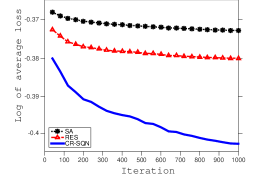
Figure 1: CR-SQN vs. RES vs. SA - $\gamma_{0}=0.01$

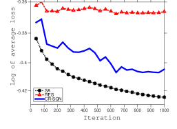
Figure 2: CR-SQN vs. RES vs. SA - $\gamma_{0}=0.1$

To perform a sensitivity analysis, we compare CR-SQN with RES and SA in Table I and II. In Table I, we report the averaged loss function of CR-SQN and RES for different settings of regularization. We maintain the initial regularization parameter of CR-SQN, $\mu_{0}$ and the regularization parameter of RES, $\mu$ to be equal. We observe that in all settings, CR-SQN attains a lower averaged loss value. In Table II, we observe that by changing the initial stepsize $\gamma_{0}$, except for the case $\gamma_{0}=0.1$, CR-SQN outperforms the SA scheme.

CR-SQN		RES
$\mu_{0}$	ave. loss	$\mu$	ave. loss
$1$	$0.6684$	$1$	$0.6839$
$0.1$	$0.6683$	$0.1$	$0.6949$
$0.01$	$0.8205$	$0.01$	$0.9017$
$0.001$	$4.3090$	$0.001$	$5.0424$

TABLE I: CR-SQN vs. RES: varying regularization parameter

CR-SQN		SA
$\gamma_{0}$	ave. loss	$\gamma_{0}$	ave. loss
$0.1$	$0.6673$	$0.1$	$0.6540$
$0.01$	$0.6683$	$0.01$	$0.6888$
$0.001$	$0.6901$	$0.001$	$0.6927$
$0.0001$	$0.6928$	$0.0001$	$0.6931$

TABLE II: CR-SQN vs. SA: varying initial stepsize

V Concluding remarks

To address stochastic optimization problems in the absence of strong convexity, we developed a cyclic regularized stochastic SQN method where at each iteration, the gradient mapping and the Hessian approximate matrix are regularized. To maintain the secant condition and carry out the convergence analysis, we do the regularization in a cyclic manner. Under specific update rules for stepsize and regularization parameters, our algorithm generates a sequence that converges to an optimal solution of the original problem in both almost sure and expected senses. Importantly, our scheme is characterized by a derived convergence rate in terms of the objective function values. Our preliminary empirical analysis on a binary classification problem is promising.

References

[1]
J. C. Spall, Introduction to Stochastic Search and Optimization:
Estimation, Simulation, and Control. Wiley, Hoboken, NJ, 2003.
[2]
Y. M. Ermoliev, “Stochastic quasigradient methods,” in Numerical
Techniques for Stochastic Optimization. Sringer-Verlag, 1983, pp. 141–185.
[3]
V. S. Borkar and S. P. Meyn, “The O.D.E. method for convergence of
stochastic approximation and reinforcement learning,” SIAM J. Control
Optim., vol. 38, no. 2, pp. 447–469 (electronic), 2000.
[4]
F. Facchinei and J.-S. Pang, Finite-dimensional variational inequalities
and complementarity problems. Vols. I,II, ser. Springer Series in
Operations Research. New York:
Springer-Verlag, 2003.
[5]
L. Bottou, “Large-scale machine learning with stochastic gradient descent,”
in Proceedings of the 19th International Conference on Computational
Statistics, Y. Lechevallier and G. Saporta, Eds. Paris, France: Springer, 2010, pp. 177–187.
[6]
R. H. Byrd, S. L. Hansen, J. Nocedal, and Y. Singer, “A stochastic
Quasi-Newton method for large-scale optimization,” 2015, arXiv:1401.7020v2
[math.OC].
[7]
R. Tibshirani, “Regression shrinkage and selection via the lasso,”
Journal of Royal Statistical Society, vol. 58, no. 1, pp. 267–288,
1996.
[8]
A. Shapiro, “Monte Carlo sampling methods,” in Handbook in Operations
Research and Management Science. Amsterdam: Elsevier Science, 2003, vol. 10, pp. 353–426.
[9]
H. Robbins and S. Monro, “A stochastic approximation method,” Ann.
Math. Statistics, vol. 22, pp. 400–407, 1951.
[10]
A. Nemirovski, A. Juditsky, G. Lan, and A. Shapiro, “Robust stochastic
approximation approach to stochastic programming,” SIAM Journal on
Optimization, vol. 19, no. 4, pp. 1574–1609, 2009.
[11]
F. Yousefian, A. Nedić, and U. V. Shanbhag, “Self-tuned stochastic
approximation schemes for non-Lipschitzian stochastic multi-user
optimization and nash games,” IEEE Transactions on Automatic
Control, 2015, to appear.
[12]
D. C. Liu and J. Nocedal, “On the limited memory bfgs method for large scale
optimization,” Math. Program., vol. 45, no. 3, pp. 503–528, Dec.
1989. [Online]. Available: http://dx.doi.org/10.1007/BF01589116
[13]
J. Nocedal and S. J. Wright, Numerical Optimization, 2nd ed. New York: Springer, 2006.
[14]
D.-H. Li and M. Fukushima, “A modified BFGS method and its global
convergence in nonconvex minimization,” Journal of Computational and
Applied Mathematics, vol. 129, pp. 15–35, 2001.
[15]
A. Bordes and L. B. N. P. Gallinari, “SGD-QN: Careful quasi-newton
stochastic gradient descent,” Journal of Machine Learning Research,
vol. 10, pp. 1737–1754, 2009.
[16]
N. N. Schraudolph, J. Yu, and S. Gunter, “A stochastic quasi-newton method for
online convex optimization,” In Proc. 11th Intl. Conf. on Artificial
Intelligence and Statistics (AIstats), pp. 433–440, 2007.
[17]
A. Mokhtari and A. Ribeiro, “RES: regularized stochastic BFGS algorithm,”
IEEE Transactions on Signal Processing, vol. 62, no. 23, pp.
6089–6104, 2014.
[18]
——, “Global convergence of online limited memory BFGS,” Journal
of Machine Learning Research, vol. 16, pp. 3151–3181, 2015.
[19]
X. Wang, S. Ma, and W. Liu, “Stochastic quasi-Newton methods for nonconvex
stochastic optimization,” 2014, arXiv:1412.1196 [math.OC].
[20]
A. Lucchi, B. McWilliams, and T. Hofmann, “A variance reduced stochastic
newton method,” arXiv preprint arXiv:1503.08316 (2015).
[21]
A. Nedić and S. Lee, “On stochastic subgradient mirror-descent algorithm
with weighted averaging,” SIAM Journal on Optimization, vol. 24,
no. 1, pp. 84–107, 2014.
[22]
B. Polyak, Introduction to optimization. New York: Optimization Software, Inc., 1987.
[23]
I. C. Yeh and C. H. Lien, “The comparisons of data mining techniques for the
predictive accuracy of probability of default of credit card clients,”
Expert Systems with Applications, vol. 36, no. 2, pp. 2473–2480,
2007.