Simple and Accurate Dependency Parsing
Using Bidirectional LSTM Feature Representations

Abstract

We present a simple and effective scheme for dependency parsing which is based on bidirectional-LSTMs (BiLSTMs). Each sentence token is associated with a BiLSTM vector representing the token in its sentential context, and feature vectors are constructed by concatenating a few BiLSTM vectors. The BiLSTM is trained jointly with the parser objective, resulting in very effective feature extractors for parsing. We demonstrate the effectiveness of the approach by applying it to a greedy transition-based parser as well as to a globally optimized graph-based parser. The resulting parsers have very simple architectures, and match or surpass the state-of-the-art accuracies on English and Chinese.

1 Introduction

The focus of this paper is on feature representation for dependency parsing, using recent techniques from the neural-networks (“deep learning”) literature. Modern approaches to dependency parsing can be broadly categorized into graph-based and transition-based parsers [Kübler et al. (2009]. Graph-based parsers [McDonald (2006] treat parsing as a search-based structured prediction problem in which the goal is learning a scoring function over dependency trees such that the correct tree is scored above all other trees. Transition-based parsers [Nivre (2004, Nivre (2008] treat parsing as a sequence of actions that produce a parse tree, and a classifier is trained to score the possible actions at each stage of the process and guide the parsing process. Perhaps the simplest graph-based parsers are arc-factored (first order) models [McDonald (2006], in which the scoring function for a tree decomposes over the individual arcs of the tree. More elaborate models look at larger (overlapping) parts, requiring more sophisticated inference and training algorithms [Martins et al. (2009, Koo and Collins (2010]. The basic transition-based parsers work in a greedy manner, performing a series of locally-optimal decisions, and boast very fast parsing speeds. More advanced transition-based parsers introduce some search into the process using a beam [Zhang and Clark (2008] or dynamic programming [Huang and Sagae (2010].

Regardless of the details of the parsing framework being used, a crucial step in parser design is choosing the right feature function for the underlying statistical model. Recent work (see Section 2.2 for an overview) attempt to alleviate parts of the feature function design problem by moving from linear to non-linear models, enabling the modeler to focus on a small set of “core” features and leaving it up to the machine-learning machinery to come up with good feature combinations [Chen and Manning (2014, Pei et al. (2015, Lei et al. (2014, Taub-Tabib et al. (2015]. However, the need to carefully define a set of core features remains. For example, the work of ?) uses 18 different elements in its feature function, while the work of ?) uses 21 different elements. Other works, notably ?) and ?), propose more sophisticated feature representations, in which the feature engineering is replaced with architecture engineering.

In this work, we suggest an approach which is much simpler in terms of both feature engineering and architecture engineering. Our proposal (Section 3) is centered around BiRNNs [Irsoy and Cardie (2014, Schuster and Paliwal (1997], and more specifically BiLSTMs [Graves (2008], which are strong and trainable sequence models (see Section 2.3). The BiLSTM excels at representing elements in a sequence (i.e., words) together with their contexts, capturing the element and an “infinite” window around it. We represent each word by its BiLSTM encoding, and use a concatenation of a minimal set of such BiLSTM encodings as our feature function, which is then passed to a non-linear scoring function (multi-layer perceptron). Crucially, the BiLSTM is trained with the rest of the parser in order to learn a good feature representation for the parsing problem. If we set aside the inherent complexity of the BiLSTM itself and treat it as a black box, our proposal results in a pleasingly simple feature extractor.

We demonstrate the effectiveness of the approach by using the BiLSTM feature extractor in two parsing architectures, transition-based (Section 4) as well as a graph-based (Section 2). In the graph-based parser, we jointly train a structured-prediction model on top of a BiLSTM, propagating errors from the structured objective all the way back to the BiLSTM feature-encoder. To the best of our knowledge, we are the first to perform such end-to-end training of a structured prediction model and a recurrent feature extractor for non-sequential outputs.

Aside from the novelty of the BiLSTM feature extractor and the end-to-end structured training, we rely on existing models and techniques from the parsing and structured prediction literature. We stick to the simplest parsers in each category – greedy inference for the transition-based architecture, and a first-order, arc-factored model for the graph-based architecture. Despite the simplicity of the parsing architectures and the feature functions, we achieve near state-of-the-art parsing accuracies in both English (93.1 UAS) and Chinese (86.6 UAS), using a first-order parser with two features and while training solely on Treebank data, without relying on semi-supervised signals such as pre-trained word embeddings [Chen and Manning (2014], word-clusters [Koo et al. (2008], or techniques such as tri-training [Weiss et al. (2015]. When also including pre-trained word embeddings, we obtain further improvements, with accuracies of 93.9 UAS (English) and 87.6 UAS (Chinese) for a greedy transition-based parser with 11 features, and 93.6 UAS (En) / 87.4 (Ch) for a greedy transition-based parser with 4 features.

2 Background and Notation

Notation

We use $x_{1:n}$ to denote a sequence of $n$ vectors $x_{1},\cdots,x_{n}$. $F_{\theta}(\cdot)$ is a function parameterized with parameters $\theta$. We write $F_{L}(\cdot)$ as shorthand for $F_{\theta_{L}}$ – an instantiation of $F$ with a specific set of parameters $\theta_{L}$. We use $\circ$ to denote a vector concatenation operation, and $v[i]$ to denote an indexing operation taking the $i$th element of a vector $v$.

2.1 Feature Functions in Dependency Parsing

Traditionally, state-of-the-art parsers rely on linear models over hand-crafted feature functions. The feature functions look at core components (e.g. “word on top of stack”, “leftmost child of the second-to-top word on the stack”, “distance between the head and the modifier words”), and are comprised of several templates, where each template instantiates a binary indicator function over a conjunction of core elements (resulting in features of the form “word on top of stack is X and leftmost child is Y and …”). The design of the feature function – which components to consider and which combinations of components to include – is a major challenge in parser design. Once a good feature function is proposed in a paper it is usually adopted in later works, and sometimes tweaked to improve performance. Examples of good feature functions are the feature-set proposed by ?) for transition-based parsing (including roughly 20 core components and 72 feature templates), and the feature-set proposed by ?) for graph-based parsing, with the paper listing 18 templates for a first-order parser, while the first order feature-extractor in the actual implementation’s code (MSTParser) includes roughly a hundred feature templates.

The core features in a transition-based parser usually look at information such as the word-identity and part-of-speech (POS) tags of a fixed number of words on top of the stack, a fixed number of words on the top of the buffer, the modifiers (usually left-most and right-most) of items on the stack and on the buffer, the number of modifiers of these elements, parents of words on the stack, and the length of the spans spanned by the words on the stack. The core features of a first-order graph-based parser usually take into account the word and POS of the head and modifier items, as well as POS-tags of the items around the head and modifier, POS tags of items between the head and modifier, and the distance and direction between the head and modifier.

2.2 Related Research Efforts

Coming up with a good feature-set for a parser is a hard and time consuming task, and many researchers attempt to reduce the required manual effort. The work of ?) suggests a low-rank tensor representation to automatically find good feature combinations. ?) suggest a kernel-based approach to implicitly consider all possible feature combinations over sets of core-features. The recent popularity of neural networks prompted a move from templates of sparse, binary indicator features to dense core feature encodings fed into non-linear classifiers. ?) encode each core feature of a greedy transition-based parser as a dense low-dimensional vector, and the vectors are then concatenated and fed into a non-linear classifier (multi-layer perceptron) which can potentially capture arbitrary feature combinations. ?) showed further gains using the same approach coupled with a somewhat improved set of core features, a more involved network architecture with skip-layers, beam search-decoding, and careful hyper-parameter tuning. ?) apply a similar methodology to graph-based parsing. While the move to neural-network classifiers alleviates the need for hand-crafting feature-combinations, the need to carefully define a set of core features remain. For example, the feature representation in ?) is a concatenation of 18 word vectors, 18 POS vectors and 12 dependency-label vectors.

The above works tackle the effort in hand-crafting effective feature combinations. A different line of work attacks the feature-engineering problem by suggesting novel neural-network architectures for encoding the parser state, including intermediately-built subtrees, as vectors which are then fed to non-linear classifiers. Titov and Henderson encode the parser state using incremental sigmoid-belief networks [Titov and Henderson (2007]. In the work of ?), the entire stack and buffer of a transition-based parser are encoded as a stack-LSTMs, where each stack element is itself based on a compositional representation of parse trees. ?) encode each tree node as two compositional representations capturing the inside and outside structures around the node, and feed the representations into a reranker. A similar reranking approach, this time based on convolutional neural networks, is taken by ?). Finally, in ?) we present an Easy-First parser based on a novel hierarchical-LSTM tree encoding.

In contrast to these, the approach we present in this work results in much simpler feature functions, without resorting to elaborate network architectures or compositional tree representations.

Work by ?) employs a sequence-to-sequence with attention architecture for constituency parsing. Each token in the input sentence is encoded in a deep-BiLSTM representation, and then the tokens are fed as input to a deep-LSTM that predicts a sequence of bracketing actions based on the already predicted bracketing as well as the encoded BiLSTM vectors. A trainable attention mechanism is used to guide the parser to relevant BiLSTM vectors at each stage. This architecture shares with ours the use of BiLSTM encoding and end-to-end training. The sequence of bracketing actions can be interpreted as a sequence of Shift and Reduce operations of a transition-based parser. However, while the parser of Vinyals et al. relies on a trainable attention mechanism for focusing on specific BiLSTM vectors, parsers in the transition-based family we use in Section 4 use a human designed stack and buffer mechanism to manually direct the parser’s attention. While the effectiveness of the trainable attention approach is impressive, the stack-and-buffer guidance of transition-based parsers results in more robust learning. Indeed, work by ?), published while working on the camera-ready version of this paper, show that the same methodology as ours is highly effective also for greedy, transition-based constituency parsing, surpassing the beam-based architecture of Vinyals et al. (88.3F vs. 89.8F points) when trained on the Penn Treebank dataset and without using orthogonal methods such as ensembling and up-training.

2.3 Bidirectional Recurrent Neural Networks

Recurrent neural networks (RNNs) are statistical learners for modeling sequential data. An RNN allows one to model the $i$th element in the sequence based on the past – the elements $x_{1:i}$ up to and including it. The RNN model provides a framework for conditioning on the entire history $x_{1:i}$ without resorting to the Markov assumption which is traditionally used for modeling sequences. RNNs were shown to be capable of learning to count, as well as to model line lengths and complex phenomena such as bracketing and code indentation [Karpathy et al. (2015]. Our proposed feature extractors are based on a bidirectional recurrent neural network (BiRNN), an extension of RNNs that take into account both the past $x_{1:i}$ and the future $x_{i:n}$. We use a specific flavor of RNN called a long short-term memory network (LSTM). For brevity, we treat RNN as an abstraction, without getting into the mathematical details of the implementation of the RNNs and LSTMs. For further details on RNNs and LSTMs, the reader is referred to ?) and ?).

The recurrent neural network (RNN) abstraction is a parameterized function $\textsc{Rnn}_{\theta}(x_{1:n})$ mapping a sequence of $n$ input vectors $x_{1:n}$, $x_{i}\in\mathbb{R}^{d_{in}}$ to a sequence of $n$ output vectors $h_{1:n},h_{i}\in\mathbb{R}^{d_{out}}$. Each output vector $h_{i}$ is conditioned on all the input vectors $x_{1:i}$, and can be thought of as a summary of the prefix $x_{1:i}$ of $x_{1:n}$. In our notation, we ignore the intermediate vectors $h_{1:{n-1}}$ and take the output of $\textsc{Rnn}_{\theta}(x_{1:n})$ to be the vector $h_{n}$.

A bidirectional RNN is composed of two RNNs, $\textsc{Rnn}_{F}$ and $\textsc{Rnn}_{R}$, one reading the sequence in its regular order, and the other reading it in reverse. Concretely, given a sequence of vectors $x_{1:n}$ and a desired index $i$, the function $\textsc{BiRnn}_{\theta}(x_{1:n},i)$ is defined as:

$$\textsc{BiRnn}_{\theta}(x_{1:n},i) =\textsc{Rnn}_{F}(x_{1:i})\circ\textsc{Rnn}_{R}(x_{n:i})$$

The vector $v_{i}=\textsc{BiRnn}(x_{1:n},i)$ is then a representation of the $i$th item in $x_{1:n}$, taking into account both the entire history $x_{1:i}$ and the entire future $x_{i:n}$ by concatenating the matching Rnns. We can view the BiRNN encoding of an item $i$ as representing the item $i$ together with a context of an infinite window around it.

Computational Complexity

Computing the BiRNN vectors encoding of the $i$th element of a sequence $x_{1:n}$ requires $O(n)$ time for computing the two RNNs and concatenating their outputs. A naive approach of computing the bidirectional representation of all $n$ elements result in $O(n^{2})$ computation. However, it is trivial to compute the BiRNN encoding of all sequence items in linear time by pre-computing $\textsc{RNN}_{F}(x_{1:n})$ and $\textsc{RNN}_{R}(x_{n:1})$, keeping the intermediate representations, and concatenating the required elements as needed.

BiRNN Training

Initially, the BiRNN encodings $v_{i}$ do not capture any particular information. During training, the encoded vectors $v_{i}$ are fed into further network layers, until at some point a prediction is made, and a loss is incurred. The back-propagation algorithm is used to compute the gradients of all the parameters in the network (including the BiRNN parameters) with respect to the loss, and an optimizer is used to update the parameters according to the gradients. The training procedure causes the BiRNN function to extract from the input sequence $x_{1:n}$ the relevant information for the task task at hand.

Going deeper

We use a variant of deep bidirectional RNN (or $k$-layer BiRNN) which is composed of $k$ BiRNN functions $\textsc{BiRnn}_{1},\cdots,\textsc{BiRnn}_{k}$ that feed into each other: the output $\textsc{BiRnn}_{\ell}(x_{1:n},1),\dots,\textsc{BiRnn}_{\ell}(x_{1:n},n)$ of $\textsc{BiRnn}_{\ell}$ becomes the input of $\textsc{BiRnn}_{\ell+1}$. Stacking BiRNNs in this way has been empirically shown to be effective [Irsoy and Cardie (2014]. In this work, we use BiRNNs and deep-BiRNNs interchangeably, specifying the number of layers when needed.

Historical Notes

RNNs were introduced by ?), and extended to BiRNNs by ?). The LSTM variant of RNNs is due to ?). BiLSTMs were recently popularized by ?), and deep BiRNNs were introduced to NLP by ?), who used them for sequence tagging. In the context of parsing, ?) and ?) use a BiLSTM sequence tagging model to assign a CCG supertag for each token in the sentence. ?) feeds the resulting supertags sequence into an A* CCG parser. ?) adds an additional layer of LSTM which receives the BiLSTM representation together with the k-best supertags for each word and outputs the most likely supertag given previous tags, and then feeds the predicted supertags to a discriminitively trained parser. In both works, the BiLSTM is trained to produce accurate CCG supertags, and is not aware of the global parsing objective.

3 Our Approach

We propose to replace the hand-crafted feature functions in favor of minimally-defined feature functions which make use of automatically learned Bidirectional LSTM representations.

Given $n$-words input sentence $s$ with words $w_{1},\dots,w_{n}$ together with the corresponding POS tags $t_{1},\dots,t_{n}$, we associate each word $w_{i}$ and POS $t_{i}$ with embedding vectors $e(w_{i})$ and $e(t_{i})$, and create a sequence of input vectors $x_{1:n}$ in which each $x_{i}$ is a concatenation of the corresponding word and POS vectors:

$$x_{i}=e(w_{i})\circ e(p_{i})$$

The embeddings are trained together with the model. This encodes each word in isolation, disregarding its context. We introduce context by representing each input element as its (deep) BiLSTM vector, $v_{i}$:

$$v_{i} =\textsc{BiLstm}(x_{1:n},i)$$

Our feature function $\phi$ is then a concatenation of a small number of BiLSTM vectors. The exact feature function is parser dependent and will be discussed when discussing the corresponding parsers. The resulting feature vectors are then scored using a non-linear function, namely a multi-layer perceptron with one hidden layer (MLP):

$$MLP_{\theta}(x)=W^{2}\cdot\tanh(W^{1}\cdot x+b^{1})+b^{2}$$

where $\theta=\{W^{1},W^{2},b^{1},b^{2}\}$ are the model parameters.

Beside using the BiLSTM-based feature functions, we make use of standard parsing techniques. Crucially, the BiLSTM is trained jointly with the rest of the parsing objective. This allows it to learn representations which are suitable for the parsing task.

Consider a concatenation of two BiLSTM vectors ($v_{i}\circ v_{j}$) scored using an MLP. The scoring function has access to the words and POS-tags of $v_{i}$ and $v_{j}$, as well as the words and POS-tags of the words in an infinite window surrounding them. As LSTMs are known to capture length and sequence position information, it is very plausible that the scoring function can be sensitive also to the distance between $i$ and $j$, their ordering, and the sequential material between them.

Parsing-time Complexity

Once the BiLSTM is trained, parsing is performed by first computing the BiLSTM encoding $v_{i}$ for each word in the sentence (a linear time operation). Then, parsing proceeds as usual, where the feature extraction involves a concatenation of a small number of the pre-computed $v_{i}$ vectors.

4 Transition-based Parser

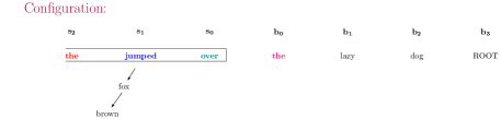
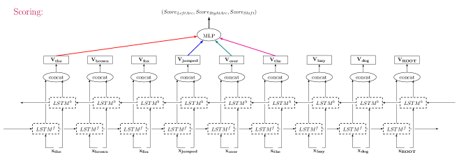
Figure 1: Illustration of the neural model scheme of the transition-based parser when calculating the scores of the possible transitions in a given configuration. The configuration (stack and buffer) is depicted on the top. Each transition is scored using an MLP that is fed the BiLSTM encodings of the first word in the buffer and the three words at the top of the stack (the colors of the words correspond to colors of the MLP inputs above), and a transition is picked greedily. Each $x_{i}$ is a concatenation of a word and a POS vector, and possibly an additional external embedding vector for the word. The figure depicts a single-layer BiLSTM, while in practice we use two layers. When parsing a sentence, we iteratively compute scores for all possible transitions and apply the best scoring action until the final configuration is reached.

We begin by integrating the feature extractor in a transition-based parser [Nivre (2008]. We follow the notation in ?). The transition-based parsing framework assumes a transition system, an abstract machine that processes sentences and produces parse trees. The transition system has a set of configurations and a set of transitions which are applied to configurations. When parsing a sentence, the system is initialized to an initial configuration based on the input sentence, and transitions are repeatedly applied to this configuration. After a finite number of transitions, the system arrives at a terminal configuration, and a parse tree is read off the terminal configuration. In a greedy parser, a classifier is used to choose the transition to take in each configuration, based on features extracted from the configuration itself. The parsing algorithm is presented in Algorithm 1 below.

Algorithm 1 Greedy transition-based parsing

1:Input: sentence $s=w_{1},\dots,x_{w},\;t_{1},\dots,t_{n}$, parameterized function $\textsc{Score}_{\mathbf{\theta}}(\cdot)$ with parameters $\mathbf{\theta}$.

2:$c\leftarrow\textsc{Initial}(s)$

3:while not $\textsc{Terminal}(c)$ do

4:   $\hat{t}\leftarrow\operatorname*{arg\,max}_{t\in\textsc{Legal}(c)}\textsc{Score}_{\mathbf{\theta}}\big{(}\phi(c),t\big{)}$

5:   $c\leftarrow\hat{t}(c)$

6:return $tree(c)$

Given a sentence $s$, the parser is initialized with the configuration $c$ (line 2). Then, a feature function $\phi(c)$ represents the configuration $c$ as a vector, which is fed to a scoring function Score assigning scores to (configuration,transition) pairs. Score scores the possible transitions $t$, and the highest scoring transition $\hat{t}$ is chosen (line 4). The transition $\hat{t}$ is applied to the configuration, resulting in a new parser configuration. The process ends when reaching a final configuration, from which the resulting parse tree is read and returned (line 6).

Transition systems differ by the way they define configurations, and by the particular set of transitions available to them. A parser is determined by the choice of a transition system, a feature function $\phi$ and a scoring function Score. Our choices are detailed below.

The Arc-Hybrid System

Many transition systems exist in the literature. In this work, we use the arc-hybrid transition system [Kuhlmann et al. (2011], which is similar to the more popular arc-standard system [Nivre (2004], but for which an efficient dynamic oracle is available [Goldberg and Nivre (2012, Goldberg and Nivre (2013]. In the arc-hybrid system, a configuration $c=(\sigma,\beta,T)$ consists of a stack $\sigma$, a buffer $\beta$, and a set $T$ of dependency arcs. Both the stack and the buffer hold integer indices pointing to sentence elements. Given a sentence $s=w_{1},\dots,w_{n},\;t_{1},\dots,t_{n}$, the system is initialized with an empty stack, an empty arc set, and $\beta=1,\dots,n,\mathtt{ROOT}$ , where $\mathtt{ROOT}$ is the special root index. Any configuration $c$ with an empty stack and a buffer containing only $\mathtt{ROOT}$ is terminal, and the parse tree is given by the arc set $T_{c}$ of $c$. The arc-hybrid system allows 3 possible transitions, Shift, $\textsc{Left}_{\ell}$ and $\textsc{Right}_{\ell}$, defined as:

$\textsc{Shift}[(\sigma,\;\;b_{0}|\beta,\;\;T)]$	$=(\sigma|b_{0},\;\;\beta,\;\;T)$
$\textsc{Left}_{\ell}[(\sigma|s_{1}|s_{0},\;\;b_{0}|\beta,\;\;T)]$	$=(\sigma|s_{1},\;\;b_{0}|\beta,\;\;T\cup\{(b_{0},s_{0},\ell)\})$
$\textsc{Right}_{\ell}[(\sigma|s_{1}|s_{0},\;\;\beta,\;\;T)]$	$=(\sigma|s_{1},\;\;\beta,\;\;T\cup\{(s_{1},s_{0},\ell)\})$

The Shift transition moves the first item of the buffer ($b_{0}$) to the stack. The Left_ℓ transition removes the first item on top of the stack ($s_{0}$) and attaches it as a modifier to $b_{0}$ with label $\ell$, adding the arc $(b_{0},s_{0},\ell)$. The Right_ℓ transition removes $s_{0}$ from the stack and attaches it as a modifier to the next item on the stack ($s_{1}$), adding the arc $(s_{1},s_{0},\ell)$.

Scoring Function

Traditionally, the scoring function $\textsc{Score}_{\mathbf{\theta}}(x,t)$ is a discriminative linear model of the form $\textsc{Score}_{W}(x,t)=(W\cdot x)[t]$. The linearity of Score required the feature function $\phi(\cdot)$ to encode non-linearities in the form of combination features. We follow Chen and Manning [Chen and Manning (2014] and replace the linear scoring model with an MLP.

$$\textsc{Score}_{\mathbf{\theta}}(x,t)=MLP_{\mathbf{\theta}}(x)[t]$$

Simple Feature Function

The feature function $\phi(c)$ is typically complex (see Section 2.1). Our feature function is the concatenated BiLSTM vectors of the top 3 items on the stack and the first item on the buffer. I.e., for a configuration $c=(\dots|s_{2}|s_{1}|s_{0},\;\;b_{0}|\dots,\;\;T)$ the feature extractor is defined as:

$$\phi(c) =v_{s_{2}}\circ v_{s_{1}}\circ v_{s_{0}}\circ v_{b_{0}}$$

$$v_{i} =\textsc{BiLstm}(x_{1:n},i)$$

This feature function is rather minimal: it takes into account the BiLSTM representations of $s_{1},s_{0}$ and $b_{0}$, which are the items affected by the possible transitions being scored, as well as one extra stack context $s_{2}$. Figure 1 depicts transition scoring with our architecture and this feature function. Note that, unlike previous work, this feature function does not take into account $T$, the already built structure. The high parsing accuracies in the experimental sections suggest that the BiLSTM encoding is capable of estimating a lot of the missing information based on the provided stack and buffer elements and the sequential content between them.

While not explored in this work, relying on only four word indices for scoring an action results in very compact state signatures, making our proposed feature representation very appealing for use in transition-based parsers that employ dynamic-programming search [Huang and Sagae (2010, Kuhlmann et al. (2011].

Extended Feature Function

One of the benefits of the greedy transition-based parsing framework is precisely its ability to look at arbitrary features from the already built tree. If we allow somewhat less minimal feature function, we could add the BiLSTM vectors corresponding to the right-most and left-most modifiers of $s_{0}$, $s_{1}$ and $s_{2}$, as well as the left-most modifier of $b_{0}$, reaching a total of 11 BiLSTM vectors. We refer to this as the extended feature set. As we’ll see in Section 6, using the extended set does indeed improve parsing accuracies when using pre-trained word embeddings, but has a minimal effect in the fully-supervised case.

4.1 Details of the Training Algorithm

The training objective is to set the score of correct transitions above the scores of incorrect transitions. We use a margin-based objective, aiming to maximize the margin between the highest scoring correct action and the highest scoring incorrect action. The hinge loss at each parsing configuration $c$ is defined as:

$$max\Big{(}0,1- \max_{t_{o}\in G}MLP\big{(}\phi(c)\big{)}[t_{o}]$$

$$+ \max_{t_{p}\in A\setminus G}MLP\big{(}\phi(c)\big{)}[t_{p}]\Big{)}$$

where $A$ is the set of possible transitions and $G$ is the set of correct (gold) transitions at the current stage. At each stage of the training process the parser scores the possible transitions $A$, incurs a loss, selects a transition to follow, and moves to the next configuration based on it. The local losses are summed throughout the parsing process of a sentence, and the parameters are updated with respect to the sum of the losses at sentence boundaries. The gradients of the entire network (including the MLP and the BiLSTM) with respect to the sum of the losses are calculated using the backpropagation algorithm. As usual, we perform several training iterations over the training corpus, shuffling the order of sentences in each iteration.

Error-Exploration and Dynamic Oracle Training

We follow ?);?) in using error exploration training with a dynamic-oracle, which we briefly describe below.

At each stage in the training process, the parser assigns scores to all the possible transitions $t\in A$. It then selects a transition, applies it, and moves to the next step. Which transition should be followed? A common approach follows the highest scoring transition that can lead to the gold tree. However, when training in this way the parser sees only configurations that result from following correct actions, and as a result tends to suffer from error propagation at test time. Instead, in error-exploration training the parser follows the highest scoring action in $A$ during training even if this action is incorrect, exposing it to configurations that result from erroneous decisions. This strategy requires defining the set $G$ such that the correct actions to take are well-defined also for states that cannot lead to the gold tree. Such a set $G$ is called a dynamic oracle. We perform error-exploration training using the dynamic-oracle defined by ?).

Aggressive Exploration

We found that even when using error-exploration, after one iteration the model remembers the training set quite well, and does not make enough errors to make error-exploration effective. In order to expose the parser to more errors, we follow an aggressive-exploration scheme: we sometimes follow incorrect transitions also if they score below correct transitions. Specifically, when the score of the correct transition is greater than that of the wrong transition but the difference is smaller than a margin constant, we chose to follow the incorrect action with probability $p_{agg}$ (we use $p_{agg}=0.1$ in our experiments).

Summary

The greedy transition-based parser follows standard techniques from the literature (margin-based objective, dynamic oracle training, error exploration, MLP-based non-linear scoring function). We depart from the literature by replacing the hand-crafted feature function over carefully selected components of the configuration with a concatenation of BiLSTM representations of a few prominent items on the stack and the buffer, and training the BiLSTM encoder jointly with the rest of the network.

5 Graph-based Parser

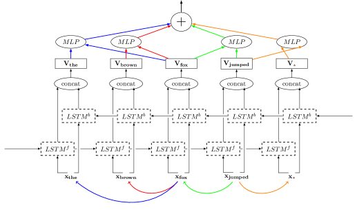
Figure 2: Illustration of the neural model scheme of the graph-based parser when calculating the score of a given parse tree. The parse tree is depicted below the sentence. Each dependency arc in the sentence is scored using an MLP that is fed the BiLSTM encoding of the words at the arc’s end points (the colors of the arcs correspond to colors of the MLP inputs above), and the individual arc scores are summed to produce the final score. All the MLPs share the same parameters. The figure depicts a single-layer BiLSTM, while in practice we use two layers. When parsing a sentence, we compute scores for all possible $n^{2}$ arcs, and find the best scoring tree using a dynamic-programming algorithm.

Graph-based parsing follows the common structured prediction paradigm [Taskar et al. (2005, McDonald et al. (2005]:

$$predict(s) =\operatorname*{arg\,max}_{y\in\mathcal{Y}(s)}score_{global}(s,y)$$

$$score_{global}(s,y) =\sum_{part\in y}score_{local}(s,part)$$

Given an input sentence $s$ (and the corresponding sequence of vectors $x_{1:n}$) we look for the highest-scoring parse tree $y$ in the space $\mathcal{Y}(s)$ of valid dependency trees over $s$. In order to make the search tractable, the scoring function is decomposed to the sum of local scores for each part independently.

In this work, we focus on arc-factored graph based approach presented in ?). Arc-factored parsing decomposes the score of a tree to the sum of the score of its head-modifier arcs $(h,m)$:

$$parse(s)=\operatorname*{arg\,max}_{y\in\mathcal{Y}(s)}\sum_{(h,m)\in y}score\big{(}\phi(s,h,m)\big{)}$$

Given the scores of the arcs the highest scoring projective tree can be efficiently found using Eisner’s decoding algorithm [Eisner (1996]. McDonald et al. and most subsequent work estimate the local score of an arc by a linear model parameterized by a weight vector $w$, and a feature function $\phi(s,h,m)$ assigning a sparse feature vector for an arc linking modifier $m$ to head $h$. We follow ?) and replace the linear scoring function with an MLP.

The feature extractor $\phi(s,h,m)$ is usually complex, involving many elements (see Section 2.1). In contrast, our feature extractor uses merely the BiLSTM encoding of the head word and the modifier word:

$$\phi(s,h,m)=\textsc{BiRnn}(x_{1:n},h)\circ\textsc{BiRnn}(x_{1:n},m)$$

The final model is:

$$parse(s) =\operatorname*{arg\,max}_{y\in\mathcal{Y}(s)}score_{global}(s,y)$$

$$=\operatorname*{arg\,max}_{y\in\mathcal{Y}(s)}\sum_{(h,m)\in y}score\big{(}\phi(s,h,m)\big{)}$$

$$=\operatorname*{arg\,max}_{y\in\mathcal{Y}(s)}\sum_{(h,m)\in y}MLP(v_{h}\circ v_{m})$$

$$v_{i} =\textsc{BiRnn}(x_{1:n},i)$$

The architecture is illustrated in Figure 2.

Training

The training objective is to set the score function such that correct tree $y$ is scored above incorrect ones. We use a margin-based objective [McDonald et al. (2005, LeCun et al. (2006], aiming to maximize the margin between the score of the gold tree $y$ and the highest scoring incorrect tree $y^{\prime}$. We define a hinge loss with respect to a gold tree $y$ as:

$$max\Big{(}0,1-\max_{y^{\prime}\neq y} \sum_{(h,m)\in y^{\prime}}{MLP(v_{h}\circ v_{m})}$$

$$+ \sum_{(h,m)\in y}{MLP(v_{h}\circ v_{m})}\Big{)}$$

Each of the tree scores is then calculated by activating the MLP on the arc representations. The entire loss can viewed as the sum of multiple neural networks, which is sub-differentiable. We calculate the gradients of the entire network (including to the BiLSTM encoder and word embeddings).

Labeled Parsing

Up to now, we described unlabeled parsing. A possible approach for adding labels is to score the combination of an unlabeled arc $(h,m)$ and its label $\ell$ by considering the label as part of the arc $(h,m,\ell)$. This results in $|Labels|\times|Arcs|$ parts that need to be scored, leading to slow parsing speeds and arguably a harder learning problem.

Instead, we chose to first predict the unlabeled structure using the model given above, and then predict the label of each resulting arc. Using this approach, the number of parts stays small, enabling fast parsing.

The labeling of an arc $(h,m)$ is performed using the same feature representation $\phi(s,h,m)$ fed into a different MLP predictor:

$$label(h,m)=\operatorname*{arg\,max}_{\ell\in labels}MLP_{LBL}(v_{h}\circ v_{m})[\ell]$$

As before we use a margin based hinge loss. The labeler is trained on the gold trees. The BiLSTM encoder responsible for producing $v_{h}$ and $v_{m}$ is shared with the arc-factored parser: the same BiLSTM encoder is used in the parer and the labeler. This sharing of parameters can be seen as an instance of multi-task learning [Caruana (1997]. As we show in Section 6, the sharing is effective: training the BiLSTM feature encoder to be good at predicting arc-labels significantly improves the parser’s unlabeled accuracy.

Loss augmented inference

In initial experiments, the network learned quickly and overfit the data. In order to remedy this, we found it useful to use loss augmented inference [Taskar et al. (2005]. The intuition behind loss augmented inference is to update against trees which have high model scores and are also very wrong. This is done by augmenting the score of each part not belonging to the gold tree by adding a constant to its score. Formally, the loss transforms as follows:

$$max(0,1+score(x,y)-$$

$$\max_{y^{\prime}\neq y}{\sum_{part\in y^{\prime}}(score_{local}(x,part)+\mathbbm{1}_{part\not\in y})})$$

Speed improvements

The arc-factored model requires the scoring of $n^{2}$ arcs. Scoring is performed using an MLP with one hidden layer, resulting in $n^{2}$ matrix-vector multiplications from the input to the hidden layer, and $n^{2}$ multiplications from the hidden to the output layer. The first $n^{2}$ multiplications involve larger dimensional input and output vectors, and are the most time consuming. Fortunately, these can be reduced to $2n$ multiplications and $n^{2}$ vector additions, by observing that the multiplication $W\cdot(v_{h}\circ v_{m})$ can be written as $W^{1}\cdot v_{h}+W^{2}\cdot v_{m}$ where $W^{1}$ and $W^{1}$ are are the first and second half of the matrix $W$ and reusing the products across different pairs.

Summary The graph-based parser is straight-forward first-order parser, trained with a margin-based hinge-loss and loss-augmented inference. We depart from the literature by replacing the hand-crafted feature function with a concatenation of BiLSTM representations of the head and modifier words, and training the BiLSTM encoder jointly with the structured objective. We also introduce a novel multi-task learning approach for labeled parsing by training a second-stage arc-labeler sharing the same BiLSTM encoder with the unlabeled parser.

6 Experiments and Results

System	Method	Representation	Emb	PTB-YM	PTB-SD		CTB
				UAS	UAS	LAS	UAS	LAS
This work	graph, 1st order	2 BiLSTM vectors	–	–	93.1	91.0	86.6	85.1
This work	transition (greedy, dyn-oracle)	4 BiLSTM vectors	–	–	93.1	91.0	86.2	85.0
This work	transition (greedy, dyn-oracle)	11 BiLSTM vectors	–	–	93.2	91.2	86.5	84.9
ZhangNivre11	transition (beam)	large feature set (sparse)	–	92.9	–	–	86.0	84.4
Martins13 (TurboParser)	graph, 3rd order+	large feature set (sparse)	–	92.8	93.1	–	–	–
Pei15	graph, 2nd order	large feature set (dense)	–	93.0	–	–	–	–
Dyer15	transition (greedy)	Stack-LSTM + composition	–	–	92.4	90.0	85.7	84.1
Ballesteros16	transition (greedy, dyn-oracle)	Stack-LSTM + composition	–	–	92.7	90.6	86.1	84.5
This work	graph, 1st order	2 BiLSTM vectors	YES	–	93.0	90.9	86.5	84.9
This work	transition (greedy, dyn-oracle)	4 BiLSTM vectors	YES	–	93.6	91.5	87.4	85.9
This work	transition (greedy, dyn-oracle)	11 BiLSTM vectors	YES	–	93.9	91.9	87.6	86.1
Weiss15	transition (greedy)	large feature set (dense)	YES	–	93.2	91.2	–	–
Weiss15	transition (beam)	large feature set (dense)	YES	–	94.0	92.0	–	–
Pei15	graph, 2nd order	large feature set (dense)	YES	93.3	–	–	–	–
Dyer15	transition (greedy)	Stack-LSTM + composition	YES	–	93.1	90.9	87.1	85.5
Ballesteros16	transition (greedy, dyn-oracle)	Stack-LSTM + composition	YES	–	93.6	91.4	87.6	86.2
LeZuidema14	reranking /blend	inside-outside recursive net	YES	93.1	93.8	91.5	–	–
Zhu15	reranking /blend	recursive conv-net	YES	93.8	–	–	85.7	–

Table 1: Test-set parsing results of various state-of-the-art parsing systems on the English (PTB) and Chinese (CTB) datasets. The systems that use embeddings may use different pre-trained embeddings. English results use predicted POS tags (different systems use different taggers), while Chinese results use gold POS tags. PTB-YM: English PTB, Yamada and Matsumoto head rules. PTB-SD: English PTB, Stanford Dependencies (different systems may use different versions of the Stanford converter). CTB: Chinese Treebank. reranking /blend in Method column indicates a reranking system where the reranker score is interpolated with the base-parser’s score. The different systems and the numbers reported from them are taken from: ZhangNivre11: [Zhang and Nivre (2011]; Martins13: [Martins et al. (2013]; Weiss15 [Weiss et al. (2015]; Pei15: [Pei et al. (2015]; Dyer15 [Dyer et al. (2015]; Ballesteros16 [Ballesteros et al. (2016]; LeZuidema14 [Le and Zuidema (2014]; Zhu15: [Zhu et al. (2015].

We evaluated our parsing model on English and Chinese data. For comparison purposes we follow the setup of ?).

Data

For English, we used the Stanford Dependency (SD) [de Marneffe and Manning (2008] conversion of the Penn Treebank [Marcus et al. (1993], using the standard train/dev/test splits with the same predicted POS-tags as used in ?);?). This dataset contains a few non-projective trees. Punctuation symbols are excluded from the evaluation.

For Chinese, we use the Penn Chinese Treebank 5.1 (CTB5), using the train/test/dev splits of [Zhang and Clark (2008, Dyer et al. (2015] with gold part-of-speech tags, also following [Dyer et al. (2015, Chen and Manning (2014].

When using external word embeddings, we also use the same data as ?).

Implementation Details

The parsers are implemented in python, using the PyCNN toolkit for neural network training. The code is available at the github repository https://github.com/elikip/bist-parser. We use the LSTM variant implemented in PyCNN, and optimize using the Adam optimizer [Kingma and Ba (2015]. Unless otherwise noted, we use the default values provided by PyCNN (e.g. for random initialization, learning rates etc).

The word and POS embeddings $e(w_{i})$ and $e(p_{i})$ are initialized to random values and trained together with the rest of the parsers’ networks. In some experiments, we introduce also pre-trained word embeddings. In those cases, the vector representation of a word is a concatenation of its randomly-initialized vector embedding with its pre-trained word vector. Both are tuned during training. We use the same word vectors as in ?)

During training, we employ a variant of word dropout [Iyyer et al. (2015], and replace a word with the unknown-word symbol with probability that is inversely proportional to the frequency of the word. A word $w$ appearing $\#(w)$ times in the training corpus is replaced with the unknown symbol with probability $p_{unk}(w)=\frac{\alpha}{\#(w)+\alpha}$. If a word was dropped the external embedding of the word is also dropped with probability $0.5$.

We train the parsers for up to 30 iterations, and choose the best model according to the UAS accuracy on the development set.

Hyperparameter Tuning

We performed a very minimal hyper-parameter search with the graph-based parser, and use the same hyper-parameters for both parsers. The hyper-parameters of the final networks used for all the reported experiments are detailed in Table 2.

Word embedding dimension	100
POS tag embedding dimension	25
Hidden units in $MLP$	100
Hidden units in $MLP_{LBL}$	100
BI-LSTM Layers	2
BI-LSTM Dimensions (hidden/output)	125 / 125
$\alpha$ (for word dropout)	0.25
$p_{agg}$ (for exploration training)	0.1

Table 2: Hyper-parameter values used in experiments

Main Results Table 1 lists the test-set accuracies of our best parsing models, compared to other state-of-the-art parsers from the literature.

It is clear that our parsers are very competitive, despite using very simple parsing architectures and minimal feature extractors. When not using external embeddings, the first-order graph-based parser with 2 features outperforms all other systems that are not using external resources, including the third-order TurboParser. The greedy transition based parser with 4 features also matches or outperforms most other parsers, including the beam-based transition parser with heavily engineered features of Zhang and Nivre (2011) and the Stack-LSTM parser of ?), as well as the same parser when trained using a dynamic oracle [Ballesteros et al. (2016]. Moving from the simple (4 features) to the extended (11 features) feature set leads to some gains in accuracy for both English and Chinese.

Interestingly, when adding external word embeddings the accuracy of the graph-based parser degrades. We are not sure why this happens, and leave the exploration of effective semi-supervised parsing with the graph-based model for future work. The greedy parser does manage to benefit from the external embeddings, and using them we also see gains from moving from the simple to the extended feature set. Both feature sets result in very competitive results, with the extended feature set yielding the best reported results for Chinese, and ranked second for English, after the heavily-tuned beam-based parser of ?).

Additional Results

We perform some ablation experiments in order to quantify the effect of the different components on our best models (Table 3).

	PTB		CTB
	UAS	LAS	UAS	LAS
Graph (no ext. emb)	93.3	91.0	87.0	85.4
–POS	92.9	89.8	80.6	76.8
–ArcLabeler	92.7	–	86.2	–
–Loss Aug.	81.3	79.4	52.6	51.7
Greedy (ext. emb)	93.8	91.5	87.8	86.0
–POS	93.4	91.2	83.4	81.6
–DynOracle	93.5	91.4	87.5	85.9

Table 3: Ablation experiments results (dev set) for the graph-based parser without external embeddings and the greedy parser with external embeddings and extended feature set.

Loss augmented inference is crucial for the success of the graph-based parser, and the multi-task learning scheme for the arc-labeler contributes nicely to the unlabeled scores. Dynamic oracle training yields nice gains for both English and Chinese.

7 Conclusion

We presented a pleasingly effective approach for feature extraction for dependency parsing based on a BiLSTM encoder that is trained jointly with the parser, and demonstrated its effectiveness by integrating it into two simple parsing models: a greedy transition-based parser and a globally optimized first-order graph-based parser, yielding very competitive parsing accuracies in both cases.

Acknowledgements

This research is supported by the Intel Collaborative Research Institute for Computational Intelligence (ICRI-CI) and the Israeli Science Foundation (grant number 1555/15). We thank Lillian Lee for her important feedback and efforts invested in editing this paper. We also thank the reviewers for their valuable comments.

References

- [Ballesteros et al. (2016] Miguel Ballesteros, Yoav Goldberg, Chris Dyer, and Noah A. Smith. 2016. Training with exploration improves a greedy stack-LSTM parser. CoRR, abs/1603.03793.
- [Caruana (1997] Rich Caruana. 1997. Multitask learning. Machine Learning, 28:41–75, July.
- [Chen and Manning (2014] Danqi Chen and Christopher Manning. 2014. A fast and accurate dependency parser using neural networks. In Proceedings of the 2014 Conference on Empirical Methods in Natural Language Processing (EMNLP), pages 740–750, Doha, Qatar, October. Association for Computational Linguistics.
- [Chiu and Nichols (2016] Jason P.C. Chiu and Eric Nichols. 2016. Named entity recognition with bidirectional LSTM-CNNs. Transactions of the Association for Computational Linguistics, 4. To appear.
- [Cho (2015] Kyunghyun Cho. 2015. Natural language understanding with distributed representation. CoRR, abs/1511.07916.
- [Cross and Huang (2016] James Cross and Liang Huang. 2016. Incremental parsing with minimal features using bi-directional LSTM. In Proceedings of the 54th Annual Meeting of the Association for Computational Linguistics, Berlin, Germany, August. Association for Computational Linguistics.
- [de Marneffe and Manning (2008] Marie-Catherine de Marneffe and Christopher D. Manning. 2008. Stanford dependencies manual. Technical report, Stanford University.
- [Dyer et al. (2015] Chris Dyer, Miguel Ballesteros, Wang Ling, Austin Matthews, and Noah A. Smith. 2015. Transition-based dependency parsing with stack long short-term memory. In Proceedings of the 53rd Annual Meeting of the Association for Computational Linguistics and the 7th International Joint Conference on Natural Language Processing (Volume 1: Long Papers), pages 334–343, Beijing, China, July. Association for Computational Linguistics.
- [Eisner (1996] Jason Eisner. 1996. Three new probabilistic models for dependency parsing: An exploration. In 16th International Conference on Computational Linguistics, Proceedings of the Conference, COLING 1996, Center for Sprogteknologi, Copenhagen, Denmark, August 5-9, 1996, pages 340–345.
- [Elman (1990] Jeffrey L. Elman. 1990. Finding structure in time. Cognitive Science, 14(2):179–211.
- [Goldberg and Nivre (2012] Yoav Goldberg and Joakim Nivre. 2012. A dynamic oracle for arc-eager dependency parsing. In Proceedings of COLING 2012, pages 959–976, Mumbai, India, December. The COLING 2012 Organizing Committee.
- [Goldberg and Nivre (2013] Yoav Goldberg and Joakim Nivre. 2013. Training deterministic parsers with non-deterministic oracles. Transactions of the Association for Computational Linguistics, 1:403–414.
- [Goldberg (2015] Yoav Goldberg. 2015. A primer on neural network models for natural language processing. CoRR, abs/1510.00726.
- [Graves (2008] Alex Graves. 2008. Supervised sequence labelling with recurrent neural networks. Ph.D. thesis, Technical University Munich.
- [Hochreiter and Schmidhuber (1997] Sepp Hochreiter and Jürgen Schmidhuber. 1997. Long short-term memory. Neural Computation, 9(8):1735–1780.
- [Huang and Sagae (2010] Liang Huang and Kenji Sagae. 2010. Dynamic programming for linear-time incremental parsing. In Proceedings of the 48th Annual Meeting of the Association for Computational Linguistics, pages 1077–1086, Uppsala, Sweden, July. Association for Computational Linguistics.
- [Irsoy and Cardie (2014] Ozan Irsoy and Claire Cardie. 2014. Opinion mining with deep recurrent neural networks. In Proceedings of the 2014 Conference on Empirical Methods in Natural Language Processing (EMNLP), pages 720–728, Doha, Qatar, October. Association for Computational Linguistics.
- [Iyyer et al. (2015] Mohit Iyyer, Varun Manjunatha, Jordan Boyd-Graber, and Hal Daumé III. 2015. Deep unordered composition rivals syntactic methods for text classification. In Proceedings of the 53rd Annual Meeting of the Association for Computational Linguistics and the 7th International Joint Conference on Natural Language Processing (Volume 1: Long Papers), pages 1681–1691, Beijing, China, July. Association for Computational Linguistics.
- [Karpathy et al. (2015] Andrej Karpathy, Justin Johnson, and Fei-Fei Li. 2015. Visualizing and understanding recurrent networks. CoRR, abs/1506.02078.
- [Kingma and Ba (2015] Diederik P. Kingma and Jimmy Ba. 2015. Adam: A method for stochastic optimization. In Proceedings of the 3rd International Conference for Learning Representations, San Diego, California.
- [Kiperwasser and Goldberg (2016] Eliyahu Kiperwasser and Yoav Goldberg. 2016. Easy-first dependency parsing with hierarchical tree LSTMs. Transactions of the Association for Computational Linguistics, 4. To appear.
- [Koo and Collins (2010] Terry Koo and Michael Collins. 2010. Efficient third-order dependency parsers. In Proceedings of the 48th Annual Meeting of the Association for Computational Linguistics, pages 1–11, Uppsala, Sweden, July. Association for Computational Linguistics.
- [Koo et al. (2008] Terry Koo, Xavier Carreras, and Michael Collins. 2008. Simple semi-supervised dependency parsing. In Proceedings of the 46th Annual Meeting of the Association for Computational Linguistics, pages 595–603, Columbus, Ohio, June. Association for Computational Linguistics.
- [Kübler et al. (2009] Sandra Kübler, Ryan T. McDonald, and Joakim Nivre. 2009. Dependency Parsing. Synthesis Lectures on Human Language Technologies. Morgan & Claypool Publishers.
- [Kuhlmann et al. (2011] Marco Kuhlmann, Carlos Gómez-Rodríguez, and Giorgio Satta. 2011. Dynamic programming algorithms for transition-based dependency parsers. In Proceedings of the 49th Annual Meeting of the Association for Computational Linguistics: Human Language Technologies, pages 673–682, Portland, Oregon, USA, June. Association for Computational Linguistics.
- [Lample et al. (2016] Guillaume Lample, Miguel Ballesteros, Sandeep Subramanian, Kazuya Kawakami, and Chris Dyer. 2016. Neural architectures for named entity recognition. In Proceedings of the 2016 Conference of the North American Chapter of the Association for Computational Linguistics: Human Language Technologies, pages 260–270, San Diego, California, June. Association for Computational Linguistics.
- [Le and Zuidema (2014] Phong Le and Willem Zuidema. 2014. The inside-outside recursive neural network model for dependency parsing. In Proceedings of the 2014 Conference on Empirical Methods in Natural Language Processing (EMNLP), pages 729–739, Doha, Qatar, October. Association for Computational Linguistics.
- [LeCun et al. (2006] Yann LeCun, Sumit Chopra, Raia Hadsell, Marc’Aurelio Ranzato, and Fu Jie Huang. 2006. A tutorial on energy-based learning. Predicting structured data, 1.
- [Lei et al. (2014] Tao Lei, Yu Xin, Yuan Zhang, Regina Barzilay, and Tommi Jaakkola. 2014. Low-rank tensors for scoring dependency structures. In Proceedings of the 52nd Annual Meeting of the Association for Computational Linguistics (Volume 1: Long Papers), pages 1381–1391, Baltimore, Maryland, June. Association for Computational Linguistics.
- [Lewis et al. (2016] Mike Lewis, Kenton Lee, and Luke Zettlemoyer. 2016. LSTM CCG parsing. In Proceedings of the 2016 Conference of the North American Chapter of the Association for Computational Linguistics: Human Language Technologies, pages 221–231, San Diego, California, June. Association for Computational Linguistics.
- [Marcus et al. (1993] Mitchell P. Marcus, Beatrice Santorini, and Mary Ann Marcinkiewicz. 1993. Building a large annotated corpus of English: The Penn Treebank. Computational Linguistics, 19(2):313–330.
- [Martins et al. (2009] Andre Martins, Noah A. Smith, and Eric Xing. 2009. Concise integer linear programming formulations for dependency parsing. In Proceedings of the Joint Conference of the 47th Annual Meeting of the ACL and the 4th International Joint Conference on Natural Language Processing of the AFNLP, pages 342–350, Suntec, Singapore, August. Association for Computational Linguistics.
- [Martins et al. (2013] Andre Martins, Miguel Almeida, and Noah A. Smith. 2013. Turning on the turbo: Fast third-order non-projective turbo parsers. In Proceedings of the 51st Annual Meeting of the Association for Computational Linguistics (Volume 2: Short Papers), pages 617–622, Sofia, Bulgaria, August. Association for Computational Linguistics.
- [McDonald et al. (2005] Ryan McDonald, Koby Crammer, and Fernando Pereira. 2005. Online large-margin training of dependency parsers. In Proceedings of the 43rd Annual Meeting of the Association for Computational Linguistics (ACL’05), pages 91–98, Ann Arbor, Michigan, June. Association for Computational Linguistics.
- [McDonald (2006] Ryan McDonald. 2006. Discriminative Training and Spanning Tree Algorithms for Dependency Parsing. Ph.D. thesis, University of Pennsylvania.
- [Nivre (2004] Joakim Nivre. 2004. Incrementality in deterministic dependency parsing. In Frank Keller, Stephen Clark, Matthew Crocker, and Mark Steedman, editors, Proceedings of the ACL Workshop Incremental Parsing: Bringing Engineering and Cognition Together, pages 50–57, Barcelona, Spain, July. Association for Computational Linguistics.
- [Nivre (2008] Joakim Nivre. 2008. Algorithms for deterministic incremental dependency parsing. Computational Linguistics, 34(4):513–553.
- [Pei et al. (2015] Wenzhe Pei, Tao Ge, and Baobao Chang. 2015. An effective neural network model for graph-based dependency parsing. In Proceedings of the 53rd Annual Meeting of the Association for Computational Linguistics and the 7th International Joint Conference on Natural Language Processing (Volume 1: Long Papers), pages 313–322, Beijing, China, July. Association for Computational Linguistics.
- [Schuster and Paliwal (1997] Mike Schuster and Kuldip K. Paliwal. 1997. Bidirectional recurrent neural networks. IEEE Trans. Signal Processing, 45(11):2673–2681.
- [Taskar et al. (2005] Benjamin Taskar, Vassil Chatalbashev, Daphne Koller, and Carlos Guestrin. 2005. Learning structured prediction models: A large margin approach. In Machine Learning, Proceedings of the Twenty-Second International Conference (ICML 2005), Bonn, Germany, August 7-11, 2005, pages 896–903.
- [Taub-Tabib et al. (2015] Hillel Taub-Tabib, Yoav Goldberg, and Amir Globerson. 2015. Template kernels for dependency parsing. In Proceedings of the 2015 Conference of the North American Chapter of the Association for Computational Linguistics: Human Language Technologies, pages 1422–1427, Denver, Colorado, May–June. Association for Computational Linguistics.
- [Titov and Henderson (2007] Ivan Titov and James Henderson. 2007. A latent variable model for generative dependency parsing. In Proceedings of the Tenth International Conference on Parsing Technologies, pages 144–155, Prague, Czech Republic, June. Association for Computational Linguistics.
- [Vaswani et al. (2016] Ashish Vaswani, Yonatan Bisk, Kenji Sagae, and Ryan Musa. 2016. Supertagging with LSTMs. In Proceedings of the 15th Annual Conference of the North American Chapter of the Association for Computational Linguistics (Short Papers), San Diego, California, June.
- [Vinyals et al. (2015] Oriol Vinyals, Lukasz Kaiser, Terry Koo, Slav Petrov, Ilya Sutskever, and Geoffrey E. Hinton. 2015. Grammar as a foreign language. In Advances in Neural Information Processing Systems 28: Annual Conference on Neural Information Processing Systems 2015, December 7-12, 2015, Montreal, Quebec, Canada, pages 2773–2781.
- [Weiss et al. (2015] David Weiss, Chris Alberti, Michael Collins, and Slav Petrov. 2015. Structured training for neural network transition-based parsing. In Proceedings of the 53rd Annual Meeting of the Association for Computational Linguistics and the 7th International Joint Conference on Natural Language Processing (Volume 1: Long Papers), pages 323–333, Beijing, China, July. Association for Computational Linguistics.
- [Zhang and Clark (2008] Yue Zhang and Stephen Clark. 2008. A tale of two parsers: Investigating and combining graph-based and transition-based dependency parsing. In Proceedings of the 2008 Conference on Empirical Methods in Natural Language Processing, pages 562–571, Honolulu, Hawaii, October. Association for Computational Linguistics.
- [Zhang and Nivre (2011] Yue Zhang and Joakim Nivre. 2011. Transition-based dependency parsing with rich non-local features. In Proceedings of the 49th Annual Meeting of the Association for Computational Linguistics: Human Language Technologies, pages 188–193, Portland, Oregon, USA, June. Association for Computational Linguistics.
- [Zhu et al. (2015] Chenxi Zhu, Xipeng Qiu, Xinchi Chen, and Xuanjing Huang. 2015. A re-ranking model for dependency parser with recursive convolutional neural network. In Proceedings of the 53rd Annual Meeting of the Association for Computational Linguistics and the 7th International Joint Conference on Natural Language Processing (Volume 1: Long Papers), pages 1159–1168, Beijing, China, July. Association for Computational Linguistics.