An optimal regret algorithm for bandit convex optimization

Abstract

We consider the problem of online convex optimization against an arbitrary adversary with bandit feedback, known as bandit convex optimization. We give the first $\tilde{O}(\sqrt{T})$-regret algorithm for this setting based on a novel application of the ellipsoid method to online learning. This bound is known to be tight up to logarithmic factors. Our analysis introduces new tools in discrete convex geometry.

1 Introduction

In the setting of Bandit Convex Optimization (BCO), a learner repeatedly chooses a point in a convex decision set. The learner then observes a loss which is equal to the value of an adversarially chosen convex loss function. The only feedback available to the learner is the loss — a single real number. Her goal is to minimize the regret, defined to be the difference between the sum of losses incurred and the loss of the best fixed decision (point in the decision set) in hindsight.

This fundamental decision making setting is extremely general, and has been used to efficiently model online prediction problems with limited feedback such as online routing, online ranking and ad placement, and many others (see [8] and [17] chapter 6 for applications and a detailed survey of BCO). This generality and importance is accompanied by significant difficulties: BCO allows for an adversarially chosen cost functions, and extremely limited information is available to the leaner in the form of a single scalar per iteration. The extreme exploration-exploitation tradeoff common in bandit problems is accompanied by the additional challenge of polynomial time convex optimization to make this problem one of the most difficult encountered in learning theory.

As such, the setting of BCO has been extremely well studied in recent years and the state-of-the-art significantly advanced. For example, in case the adversarial cost functions are linear, efficient algorithms are known that guarantee near-optimal regret bounds [2, 9, 18]. A host of techniques have been developed to tackle the difficulties of partial information, exploration-exploitation and efficient convex optimization. Indeed, most known optimization and algorithmic techniques have been applied, including interior point methods [2], random walk optimization [23], continuous multiplicative updates [13], random perturbation [6], iterative optimization methods [15] and many more.

Despite this impressive and the long lasting effort and progress, the main question of BCO remains unresolved: construct an efficient and optimal regret algorithm for the full setting of BCO. Even the optimal regret attainable is yet unresolved in the full adversarial setting.

A significant breakthrough was recently made by [10], who show that in the oblivious setting and in the special case of 1-dimensional BCO, $O(\sqrt{T})$ regret is attainable. Their result is existential in nature, showing that the minimax regret for the oblivious BCO setting (in which the adversary decides upon a distribution over cost functions independently of the learners’ actions) behaves as $\tilde{\Theta}(\sqrt{T})$. This result was very recently extended to any dimension by [11], still with an existential bound rather than an explicit algorithm and in the oblivious setting.

In this paper we advance the state of the art in bandit convex optimization and show the following results:

1. We show that minimax regret for the full adversarial BCO setting is $\tilde{\Theta}(\sqrt{T})$.

2. We give an explicit algorithm attaining this regret bound. Such an explicit algorithm was unknown previously even for the oblivious setting.

3. The algorithm guarantees $\tilde{\Theta}(\sqrt{T})$ regret with high probability and exponentially decaying tails. Specifically, the algorithm guarantees regret of $\tilde{\Theta}(\sqrt{T}\log\frac{1}{\delta})$ with probability at least $1-\delta$.

It is known that any algorithm for BCO must suffer regret $\Omega(\sqrt{T})$ in the worst case, even for oblivious adversaries and linear cost functions. Thus, up to logarithmic factors, our results close the gap of the attainable regret in terms of the number of iterations.

To obtain these results we introduce some new techniques into online learning, namely a novel online variant of the ellipsoid algorithm, and define some new notions in discrete convex geometry.

What remains open?

Our algorithms depend exponentially on the dimensionality of the decision set, both in terms of regret bounds as well as in computational complexity. As of the time of writing, we do not know whether this dependencies are tight or can be improved to be polynomial in terms of the dimension, and we leave it as an open problem to resolve this question.

1.1 Prior work

The best known upper bound in the regret attainable for adversarial BCO with general convex loss functions is $\tilde{O}(T^{5/6})$ due to [15] and [21] . A lower bound of $\Omega(\sqrt{T})$ is folklore, even the easier full-information setting of online convex optimization, see e.g. [17].

The special case of bandit linear optimization (BCO in case where the adversary is limited to using linear losses) is significantly simper. Informally, this is since the average of the function value on a sphere around a center point equals the value of the function in the center, regardless of how large is the sphere. This allows for very efficient exploration, and was first used by [13] to devise the Geometric Hedge algorithm that achieves an optimal regret rate of $\tilde{O}(\sqrt{T})$. An efficient algorithm inspired by interior point methods was later given by [2] with the same optimal regret bound. Further improvements in terms of the dimension and other constants were subsequently given in [9, 18].

The first gradient-descent-based method for BCO was given by [15]. Their regret bound was subsequently improved for various special cases of loss functions using ideas from [2]. For convex and smooth losses, [24] attained an upper bound on the regret of of $\tilde{O}(T^{2/3})$. This was recently improved to by [14] to $\tilde{O}(T^{5/8})$. [3] obtained a regret bound of $\tilde{O}(T^{2/3})$ for strongly-convex losses. For the special case of strongly-convex and smooth losses, [3] obtained a regret of $\tilde{O}(\sqrt{T})$ in the unconstrained case, and [19] obtain the same rate even in the constrained cased. [25] gives a lower bound of $\Omega(\sqrt{T})$ for the setting of strongly-convex and smooth BCO.

A comprehensive survey by Bubeck and Cesa-Bianchi [8], provides a review of the bandit optimization literature in both stochastic and online setting.

Another very relevant line of work is that on zero-order convex optimization. This is the setting of convex optimization in which the only information available to the optimizer is a valuation oracle that given $x\in\mathcal{K}$ for some convex set $\mathcal{K}\subseteq{\mathbb{R}}^{d}$, returns $f(x)$ for some convex function $f:\mathcal{K}\mapsto{\mathbb{R}}$ (or a noisy estimate of this number). This is considered one of the hardest areas in convex optimization (although strictly a special case of BCO), and a significant body of work has culminated in a polynomial time algorithm, see [12]. Recently, [4] give a polynomial time algorithm for regret minimization in the stochastic setting of zero-order optimization, greatly improving upon the known running times.

1.2 Paper structure

In the next section we give some basic definitions and constructs that will be of use. In section 3 we survey a natural approach, motivated by zero-order optimization, and explain why completely new tools are necessary to apply it. We proceed to give the new mathematical constructions for discrete convex geometry in section 4. This is followed by our main technical lemma, the discretization lemma, in section 5. We proceed to give the new algorithm and the main result statement in section 6.

2 Preliminaries

The setting of bandit convex optimization (BCO) is a repeated game between an online learner and an adversary (see e.g. [17] chapter 6). Iteratively, the learner makes a decision which is a point in a convex decision set, which is a subset of Euclidean space $x_{t}\in\mathcal{K}\subseteq{\mathbb{R}}^{d}$. Meanwhile, the adversary responds with an arbitrary Lipschitz convex loss function $f_{t}:\mathcal{K}\mapsto{\mathbb{R}}$. The only feedback available to the learner is the loss, $f_{t}(x_{t})\in{\mathbb{R}}$, and her goal is to minimize regret, defined as

$$\mathcal{R}_{T}=\sum_{t}f_{t}(x_{t})-\min_{x^{*}\in\mathcal{K}}\sum_{t}f_{t}(x^{*})$$

Let $\mathcal{K}\subseteq{\mathbb{R}}^{d}$ be a convex compact and closed subset in Euclidean space. We denote by ${\mathcal{E}}_{\mathcal{K}}$ the minimal volume enclosing ellipsoid (MVEE) in $\mathcal{K}$, also known as the John ellipsoid [20, 7]. For simplicity, assume that ${\mathcal{E}}_{\mathcal{K}}$ is centered at zero.

Given an ellipsoid ${\mathcal{E}}=\{\sum_{i}\alpha_{i}v_{i}\,:\,\sum_{i}\alpha_{i}^{2}\leq 1\}$, we shall use the notation $\|x\|_{{\mathcal{E}}}\equiv\sqrt{x^{\top}(VV^{\top})^{-1}x}$ to denote the (Minkowski) semi-norm defined by the ellipsoid, where $V$ is the matrix with the vectors $v_{i}$’s as columns.

John’s theorem says that if we shrink MVEE of $\mathcal{K}$ by a factor of $1/d$, then it will be inside $\mathcal{K}$. For connivence, we denote by $\|\cdot\|_{\mathcal{K}}$ the norm according to $\frac{1}{d}{\mathcal{E}}_{\mathcal{K}}$, which is the matrix norm corresponding to the (shrinked by factor $1/d$) MVEE ellipsoid of $\mathcal{K}$ . To be specific, Let ${\mathcal{E}}$ be the MVEE of $\mathcal{K}$,

$$\|x\|_{\mathcal{K}}=d\|x\|_{{\mathcal{E}}}=\|x\|_{\frac{1}{d}{\mathcal{E}}}$$

We use $d\|x\|_{{\mathcal{E}}}$ inside of $\|x\|_{{\mathcal{E}}}$ merely to insure $\forall x\notin\mathcal{K}$, $\|x\|_{\mathcal{K}}\geq 1$, which simplifies our expression.

Enclosing box.

Denote by $C_{\mathcal{K}}$ the bounding box of the ellipsoid ${\mathcal{E}}_{\mathcal{K}}$, which is obtained by the box with axis parallel to the eigenpoles of ${\mathcal{E}}_{\mathcal{K}}$. The containing box $C_{\mathcal{K}}$ can be computed by first computing ${\mathcal{E}}_{\mathcal{K}}$, then the diagonal transformation of this ellipsoid into a ball, computing the minimal enclosing cube of this ball, and performing the inverse diagonal transformation into a box.

Definition 2.1 (Minkowski Distance of a convex set).

Given a convex set $\mathcal{K}\subset{\mathbb{R}}^{d}$ and $x\in{\mathbb{R}}^{d}$, the Minkowski distance $\gamma(x,\mathcal{K})$ is defined as

$$\gamma(x,\mathcal{K})=||x-x_{0}||_{\mathcal{K}-x_{0}}$$

Where $x_{0}$ is the center of the MVEE of $\mathcal{K}$. $\mathcal{K}-x_{0}$ denotes shifting $\mathcal{K}$ by $-x_{0}$ (so its MVEE is centered at zero)

Definition 2.2 (Scaled set).

For $\beta>0$, define $\beta\mathcal{K}$ as the scaled set

$$\beta\mathcal{K}=\{y\mid\gamma(y,\mathcal{K})\leq\beta\}$$

Henceforth we will require a discrete representation of convex sets, which we call grids, as constructed in Algorithm 1.

Algorithm 1 construct grid

1:  Input: convex set ${\mathcal{K}}\in{\mathbb{R}}^{d}$, resolution $\alpha$.

2:  Compute the MVEE ${\mathcal{E}}^{\prime}$ of ${\mathcal{K}}$. Let ${\mathcal{E}}=\frac{1}{d}{\mathcal{E}}^{\prime}$

3:  Let $A$ be the (unique) linear transformation such that $A({\mathcal{E}})=\mathbb{B}_{\alpha}(0)$ (unit ball of radius $\alpha$ centered at 0).

4:  Let $\mathcal{Z}^{d}=\{(x_{1},...,x_{d}),\ x_{i}\in Z\}$ be $d$-dimensional integer lattice.

5:  Output: $\operatorname{grid}=A^{-1}(\mathcal{Z})\cap{\mathcal{K}}$.

Claim 2.1.

For every $\mathcal{K}\in{\mathbb{R}}^{d}$, $\operatorname{grid}=\operatorname{grid}(\mathcal{K},\alpha)$ contains at most $(2d\alpha)^{d}$ many points

Lemma 2.1 (Property of the grid).

Let ${\mathcal{K}}^{\prime}\subseteq\mathcal{K}\subseteq{\mathbb{R}}^{d}$ be two convex sets. For every $\beta,\gamma$ such that $\beta>\gamma>1$, $\beta>d$, for every $\alpha\geq 2(\gamma+1)\beta^{2}\sqrt{d}$ such that the following holds. Let $\operatorname{grid}=\operatorname{grid}(\beta{\mathcal{K}}^{\prime}\cap\mathcal{K},\alpha)$, then we have:

1. For every $x\in{\mathcal{K}}^{\prime}$: $\exists x_{g}\in\operatorname{grid}$ such that $x_{g}+\gamma(x_{g}-x)\in\frac{1}{2\beta}{{\mathcal{K}}^{\prime}}$

2. For every $x\notin{\mathcal{K}}^{\prime}$, $x\in{\mathcal{K}}$: $\exists x_{g}\in\operatorname{grid}$ such that $x_{g}+\frac{\gamma}{\gamma(x,{\mathcal{K}}^{\prime})}(x_{g}-x)\in\frac{1}{2\beta}{{\mathcal{K}}^{\prime}}$

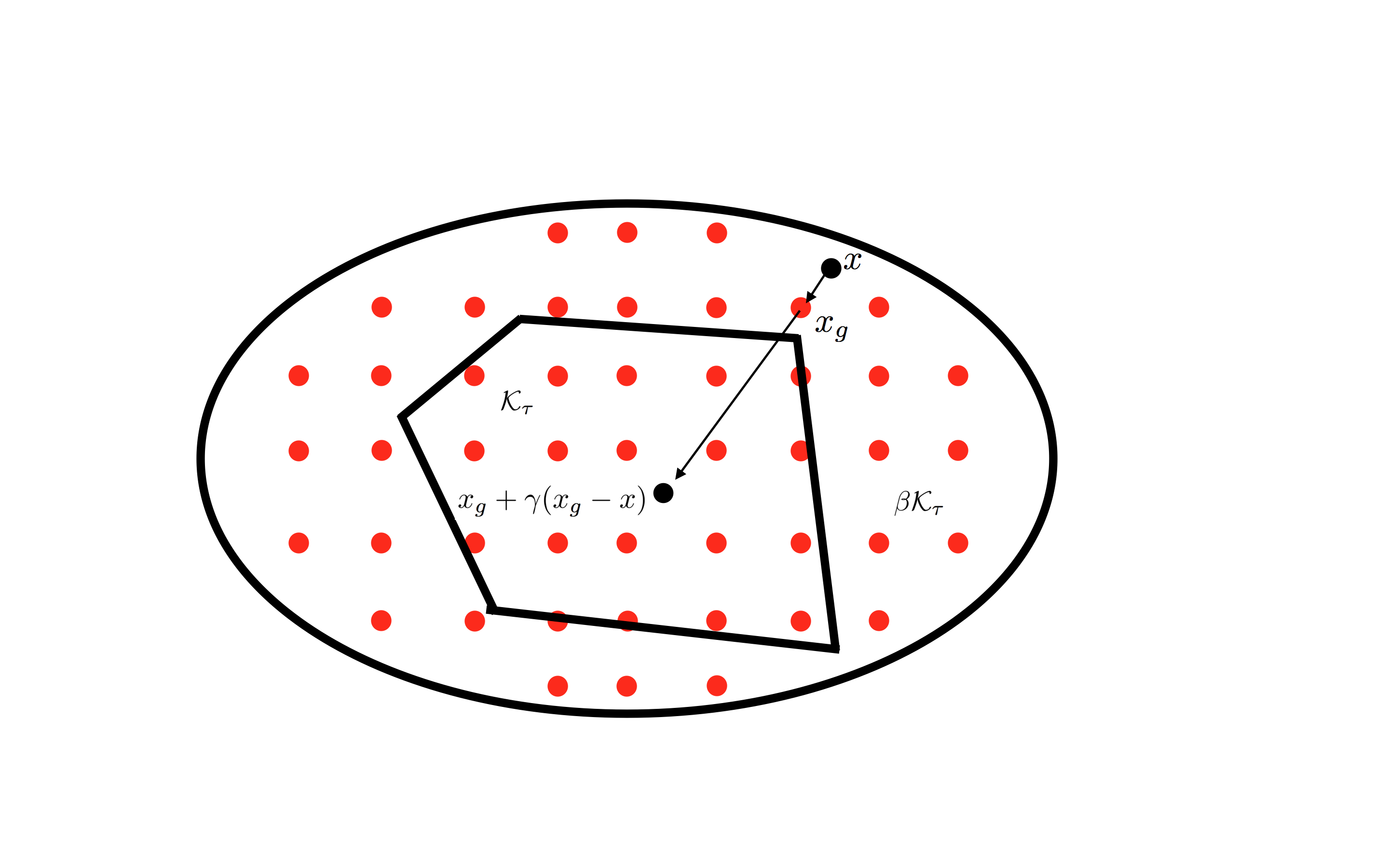
Figure 1: The property of the grid

Proof of Lemma 2.1.

Since $\beta>d$, by John’s theorem, $\mathcal{K}^{\prime}\subset\beta\mathcal{K}^{\prime}$. Moreover, since we only interested in the distance ratio, we can assume that the MVEE ${\mathcal{E}}^{\prime}$ of $\beta{\mathcal{K}}^{\prime}\cap\mathcal{K}$ is the ball centered at $0$ of radius $d\alpha$, and $\operatorname{grid}$ are all the integer points intersected with $\beta{\mathcal{K}}^{\prime}\cap\mathcal{K}$. Let ${\mathcal{E}}=\frac{1}{d}{\mathcal{E}}^{\prime}=\mathbb{B}_{\alpha}(0)$, by John’s Theorem, we know that ${\mathcal{E}}\subseteq\beta{\mathcal{K}}^{\prime}\cap\mathcal{K}\subseteq d{\mathcal{E}}$.

(a). For every $x\in{\mathcal{K}}^{\prime}$, consider point $z=\frac{\gamma}{\gamma+1}x$. Since ${\mathcal{E}}=\mathbb{B}_{\alpha}(0)\subseteq\beta{\mathcal{K}}^{\prime}$, we know that $\mathbb{B}_{\frac{\alpha}{\beta}}(0)\subseteq\mathcal{K}^{\prime}$. Therefore, $\mathbb{B}_{\frac{\alpha}{\gamma\beta}}(z)\subseteq\mathcal{K}^{\prime}$, which implies when $\alpha\geq\gamma\beta\sqrt{d}$, we can find $x_{g}\in\operatorname{grid}$ such that $\|x_{g}-z\|_{2}\leq\sqrt{d}$. Therefore,

$$\|x_{g}+\gamma(x_{g}-x)\|_{2} = \|\left[z+\gamma(z-x)\right]+\left[x_{g}-z+\gamma(x_{g}-z)\right]\|_{2}$$

$$= ||x_{g}-z+\gamma(x_{g}-z)||_{2}\quad\quad\mbox{ since $z+\gamma(z-x)=0$}$$

$$= (\gamma+1)\|x_{g}-z\|_{2}\leq(\gamma+1)\sqrt{d}\quad\quad\mbox{ by $\|x_{g}-z\|\leq\sqrt{d}$}$$

Moreover, $\frac{1}{2\beta}{\mathcal{K}}\supseteq\frac{1}{2\beta^{2}}{\mathcal{E}}=\frac{1}{2\beta^{2}}\mathbb{B}_{\alpha}(0)$ contains all points with norm $\frac{\alpha}{2\beta^{2}}$, and in particular it contains $x_{g}+\gamma(x_{g}-x)$ when $\alpha\geq 2(\gamma+1)\beta^{2}\sqrt{d}$.

(b). For every $x\notin{\mathcal{K}}^{\prime}$ but $x\in\mathcal{K}$, take $z=\frac{\gamma}{\gamma(x,{\mathcal{K}}^{\prime})+\gamma}x$. When $\beta>2\gamma$, we know that $z\in\frac{1}{2}\beta\mathcal{K}^{\prime}$. With same idea as (a), we can also conclude that

$$\mathbb{B}_{\frac{\gamma(x,{\mathcal{K}}^{\prime})}{\gamma(x,{\mathcal{K}}^{\prime})+\gamma}\frac{\alpha}{\beta^{2}}}(z)\subseteq\beta{\mathcal{K}}^{\prime}\cap\mathcal{K}$$

Since $\gamma(x,{\mathcal{K}}^{\prime})\geq 1$ for $x\notin\mathcal{K}^{\prime}$, we can find $x_{g}\in\operatorname{grid}$ be such that $\|x_{g}-z\|_{2}\leq\sqrt{d}$ when $\alpha\geq(\gamma+1)\beta^{2}\sqrt{d}$. Therefore,

$$\left\|x_{g}+\frac{\gamma}{\gamma(x,{\mathcal{K}})}(x_{g}-x)\right\|_{2}$$

$$= \left\|\left[z+\frac{\gamma}{\gamma(x,{\mathcal{K}})}(z-x)\right]+\left[x_{g}-z+\frac{\gamma}{\gamma(x,{\mathcal{K}})}(x_{g}-z)\right]\right\|_{2}$$

$$= \left\|x_{g}-z+\frac{\gamma}{\gamma(x,{\mathcal{K}})}(x_{g}-z)\right\|_{2}\quad\quad\mbox{ since $z+\frac{\gamma}{\gamma(x,{\mathcal{K}})}(z-x)=0$}$$

$$= \left(1+\frac{\gamma}{\gamma(x,{\mathcal{K}})}\right)\|x_{g}-z\|_{2}\leq\left(\frac{\gamma}{\gamma(x,{\mathcal{K}})}+1\right)\sqrt{d}$$

$$\leq (1+{\gamma})\sqrt{d}\quad\quad\mbox{ since $\gamma(x,{\mathcal{K}})\geq 1$}$$

As before, this implies that when $\alpha\geq 2(\gamma+1)\beta^{2}\sqrt{d}$, it holds that $x_{g}+\frac{\gamma}{\gamma(x,{\mathcal{K}})}(x_{g}-x)\in\frac{1}{2\beta}{{\mathcal{K}}}$.

∎

2.1 Non-stochastic bandit algorithms

Define the following

$$(p_{t},v_{t},\sigma_{t})\leftarrow\mathcal{A}(S,\{p_{t-1},f_{1:t-1}\})$$

$p_{t}$: A probability distribution over the discrete set $S$

$v_{t}$: Estimation of the values of $F^{t}=\sum_{i=1}^{t}f_{i}$ on $S$.

$\sigma_{t}$: Variance, such that for every $x\in S$, $v_{t}(x)-\sigma_{t}(x)\leq F_{t}(x)\leq v_{t}(x)+\sigma_{t}(x)$.

For $x_{t}$ picking according to distribution $p_{t}$, define the regret of $\mathcal{A}$ as:

$$\mathcal{R}_{T}=\sum_{t}f_{t}(x_{t})-\min_{x}\left\{\sum_{t}f_{t}(x)\right\}$$

The following theorem was essentially established in [5] (although the original version was stated for gains instead of losses, and had known horizon parameter), for the algorithm called EXP3.P, which is given in Appendix 8 for completeness:

Theorem 2.1 ([5]).

Algorithm EXP3.P over $N$ arms guarantees that with probability at least $1-\delta$,

$$\mathcal{R}_{T}=\sum_{t}f_{t}(x_{t})-\min_{x}\left\{\sum_{t}f_{t}(x)\right\}\leq 8\sqrt{TN\log\frac{TN}{\delta}}$$

3 The insufficiency of convex regression

Before proceeding to give the main technical contributions of this paper, we give some description of the technical difficulties that are encountered and intuition as to how they are resolved.

A natural approach for BCO, and generally for online learning, is to borrow ideas from the less general setting of stochastic zero-order optimization. Till recently, the only polynomial time algorithm for zero-order optimization was based on the ellipsoid method [16]. Roughly speaking, the idea is to maintain a subset, usually an ellipsoid, in space in which the minimum resides, and iteratively reduce the volume of this region till it is ultimately found.

In order to reduce the volume of the ellipsoid one has to find a hyperplane separating the minimum and a large constant fraction of the current ellipsoid in terms of volume. In the stochastic case, such a hyperplane can be found by sampling and estimating a sufficiently indicative region of space. A simple way to estimate the underlying convex function in the stochastic setting is called convex regression (although much more time and query-efficient methods are known, e.g. [4]).

Formally, given noisy observations from a convex function $f:\mathcal{K}\mapsto{\mathbb{R}}^{d}$, denoted $\{v(x_{1}),...,v(x_{n})\}$, such that $v(x_{i})$ is a random variable whose expectation is $f(x_{i})$, the problem of convex regression is to create an estimator of the value of $f$ over the entire space which is consistent, i.e. approaches its expectation as the number of observations increases $n\mapsto\infty$. The methodology of convex regression proceeds by solving a convex program to minimize the mean square error and ensuring convexity by adding gradient constraints, formally,

$$\min\sum_{i=1}^{n}(v(x_{i})-y_{i})^{2}$$

$$y_{j}\geq y_{i}+\nabla_{i}^{\top}(x_{j}-x_{i})$$

In this convex program $\{\nabla_{i},y_{i}\}$ are variables, points $x_{i}$ are chosen by the algorithm designer to observe, and $v(x_{i})$ the observed values from sampling. Intuitively, there are $nd+n$ degrees of freedom ($n$ scalars and $n$ vectors in $d$ dimensions) and $O(n^{2})$ constraints, which ensures that this convex program has a unique solution and generates a consistent estimator for the values of $f$ w.h.p. (see [22] for more details).

The natural approach of iteratively applying convex regression to find a separating hyperplane within an ellipsoid algorithm fails for BCO because of the following difficulties:

1. The ellipsoid method was thus far not applied successfully in online learning, since the optimum is not fixed and can change in response to the algorithms’ behavior. Even within a particular ellipsoid, the optimal strategy is not stationary.

2. Estimation using convex regression over a fixed grid is insufficient, since arbitrarily deep “valleys” can hide between the grid points.

Our algorithm and analysis below indeed follows the general ellipsoidal scheme, and overcomes these difficulties by:

1. The ellipsoid method is applied with an optional “restart button”. If the algorithm finds that the optimum is not within the current ellipsoidal set, it restarts from scratch. We show that by the time this happens, the algorithm has accumulated so much negative regret that it only helps the player. Further, inside each ellipsoid we use the standard multiarmed bandit algorithm EXP3.P due to [5], to exploit and explore it.

2. A new estimation procedure is required to ensure that no valleys are missed. For this reason we develop some new machinery in convex geometry and convex regression that we call the lower convex envelope of a function. This is a convex lower bound on the original function that ensures there are no valleys missed, and in addition needs only constant-precision grids for being consistent with the original function.

   This contribution is the most technical part of the paper, as culminates in the ”discretization lemma”, and can be skimmed at first read.

4 Geometry of discrete convex function

4.1 Lower convex envelopes of continuous and discrete convex functions

Bandit algorithms generate a discrete set of evaluations, which we have to turn into convex functions. The technical definitions that allow this are called lower convex envelopes (LCE), which we define below. First, for continuous but non-convex function $f$, we can define the LCE denoted $F_{\textsf{LCE}}(f)$ as the maximal convex function that bounds $f$ from below, or formally,

Definition 4.1 (Simple Lower Convex Envelope).

Given a function $f:\mathcal{K}\to{\mathbb{R}}$ (not necessarily convex) where $\mathcal{K}\subset{\mathbb{R}}^{d}$, the simple lower convex envelope $F_{\textsf{SLCE}}=\textsf{SLCE}(f):\mathcal{K}\to{\mathbb{R}}$ is a convex function defined as:

$$F_{\textsf{SLCE}}(x)=\min\left\{\sum_{i=1}^{s}\lambda_{i}f(y_{i})\ \right|\ \left.\exists s\in\mathbb{N}^{*},y_{1},...,y_{s}\in\mathcal{K}:\exists(\lambda_{1},...,\lambda_{s})\in\Delta^{s},x=\sum_{i}\lambda_{i}y_{i}\right\}$$

It can be seen that $F_{\textsf{SLCE}}$ is always convex, by showing for every $x,y\in\mathcal{K}$ that $f(\frac{1}{2}x+\frac{1}{2}y)\leq\frac{1}{2}f(x)+\frac{1}{2}f(y)$, which follows from the definition. Further, for a convex function, $F_{\textsf{SLCE}}(f)=f$, since for a convex function any convex combination of points satisfy $f(\sum_{i}\lambda_{i}y_{i})\leq\sum_{i}\lambda_{i}f(y_{i})$, and the minimum in the definition is realized at the point $x$ itself.

For a discrete function, the SLCE is defined to be the SLCE of the piecewise linear continuation.

We will henceforth need a significant generalization of this notion, both for the setting above, and for the setting in which the discrete function is given as a random variable - on each point in the grid we have a value estimation and variance estimate. We first define the minimal extension, and then the SLCE of this minimal extension.

Definition 4.2 (Random Discrete Function).

A Random Discrete Function (RDF), denoted $(X,v,\sigma)$, is a mapping $f:X\to{\mathbb{R}}^{2}$ on a discrete domain $X=\{x_{1},...,x_{k}\}\subseteq\mathcal{K}\subseteq{\mathbb{R}}^{d}$, and range of values and variances denoted $\{v(x),\sigma(x),x\in X\}$ such that $f(x_{i})=(v(x_{i}),\sigma(x_{i}))$.

Definition 4.3 (Minimal Extension of a Random Discrete Function).

Given a RDF $(X,v,\sigma)$, we define $\tilde{f}^{i}_{\min}(X,v,\sigma):\mathcal{K}\to{\mathbb{R}}$ as

$$\tilde{f}^{i}_{\min}(x)=\min_{h\in{\mathbb{R}}^{d}:\forall x_{j},\langle h,x_{j}-x_{i}\rangle\leq v(x_{j})+\sigma(x_{j})-[v(x_{i})-\sigma(x_{i})]}\left\{\langle h,x-x_{i}\rangle+[v(x_{i})-\sigma(x_{i})]\right\}$$

The minimal extension $\tilde{f}_{\min}(X,v,\sigma)$ is now defined as

$$\tilde{f}_{\min}(x)=\max_{i\in[k]}\tilde{f}^{i}_{\min}(x)$$

We can now define the LCE of a discrete random function

Definition 4.4 (Lower convex envelope of a random discrete function).

Given a RDF $(X,v,\sigma)$ over domain $X=\operatorname{grid}\subseteq\mathcal{K}\subseteq{\mathbb{R}}^{d}$, for the grid for $\mathcal{K}$ as constructed in Algorithm 1, its lower convex envelope is defined to be

$$F_{\textsf{LCE}}(X,v,\sigma)=F_{\textsf{SLCE}}(\tilde{f}_{\min}(X,v,\sigma))$$

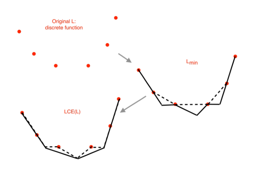
Figure 2: The minimal extension and LCE of a discrete function

We now address the question of computation of an LCE of a discrete function, or how to provide oracle access to the LCE efficiently. The following theorem and algorithm establish the computational part of this section, whose proof is deferred to the appendix.

Algorithm 2 Fit-LCE

1:  Input: RDF $(X,v,\sigma)$, and a convex set ${\mathcal{K}}$ where $X\subseteq{\mathcal{K}}$.

2:  (minimal extension): Compute the minimal extension $\tilde{f}_{\min}(X,v,\sigma):\mathcal{C}_{{\mathcal{K}}}\to{\mathbb{R}}$ (see Section 2 for definition of the bounding box $\mathcal{C}$)

3:  (LCE) Compute and return $F_{\textsf{LCE}}=\textsf{SLCE}(\tilde{f}_{\min})$.

Theorem 4.1 (LCE computation).

Given a discrete random function over $k$ points $\{x_{1},...,x_{k}\}$ in a polytope $\mathcal{K}\subseteq{\mathbb{R}}^{d}$ defined by $N=\mathop{\mbox{\rm poly}}(d)$ halfspaces, with confidence intervals $[v(x_{i})-\sigma(x_{i}),v(x_{i})+\sigma(x_{i})]$ for each point $x_{i}$, then for every $x\in\mathcal{K}$, the value $F_{\textsf{LCE}}(x)$ can be computed in time $O\left(k^{d^{2}}\right)$

To prove the running time of LCE computation, we need the following Lemma:

Lemma 4.1 (LCE properties).

The lower convex envelope (LCE) has the follow properties:

1. $\tilde{f}_{\min}$ is a piece-wise linear function with $k^{O(d^{2})}$ different regions, each region is a polytope with $d+1$ vertices. We denote all the vertices of all regions as $v_{1},...,v_{n}$ where $n=k^{O(d^{2})}$, where each $v_{i}$ and its value $\tilde{f}_{\min}(v_{i})$ are computable in time $k^{O(d^{2})}$.

2. $$F_{\textsf{LCE}}(x)=\min\left\{\sum_{i\in[n]}\lambda_{i}\tilde{f}_{\min}(v_{i})\right|\left.\sum_{i\in[n]}\lambda_{i}v_{i}=x,(\lambda_{1},...,\lambda_{n})\in\Delta^{n}\right\}$$

Proof.

Recall the definition of $\tilde{f}^{i}_{\min}:{\mathcal{K}}\to{\mathbb{R}}$ as

$$\tilde{f}^{i}_{\min}(x)=\min_{h\in{\mathbb{R}}^{d}:\forall x_{j},\langle h,x_{j}-x_{i}\rangle\leq v(x_{j})+\sigma(x_{j})-[v(x_{i})-\sigma(x_{i})]}\left\{\langle h,x-x_{i}\rangle+[v(x_{i})-\sigma(x_{i})]\right\}$$

The vector $h$ in the above expression is the result of a linear program. Therefore, it belongs to the vertex set of the polyhedral set given by the inequalities $\langle h,x_{j}-x_{i}\rangle\leq v(x_{j})+\sigma(x_{j})-[v(x_{i})-\sigma(x_{i})]$, or the objective is unbounded, a case which we can ignore since $\tilde{f}_{\min}$ is finite. The number of vertices of a polyhedral set in ${\mathbb{R}}^{d}$ defined by $k$ hyperplanes is bounded by ${k\choose d}\leq k^{d}$.

Thus, $\tilde{f}^{i}_{\min}$ is the minimal of a finite set of linear functions at any point in space. This implies that it is a piecewise linear function with at most $k^{d}$ regions. More generally, the minimum of $s$ linear functions is a piece-wise linear function of at most $s$ regions, as we now prove:

Lemma 4.1.

The minimum (or maximum) of $s$ linear functions is a piecewise linear function with at most $s$ regions.

Proof.

Let $f(x)=\min_{i\in[s]}f_{i}(x)$ for linear functions $\{f_{i}\}$, the proof for $\max_{i\in[s]}f_{i}(x)$ is analoguous. Consider the sets $S_{i}=\{x\mid f(x)=f_{i}(x)\}$, inside which $f=f_{i}$ is linear. It suffices to show that each $S_{i}$ is a convex set, and thus each $S_{i}$ is a polyhedral region with at most $s$ faces. Now suppose $x_{1},x_{2}\in S_{i}$, we want to argue that $x_{3}=\frac{x_{1}+x_{2}}{2}\in S_{i}$: Observe that for every $j$, $f_{j}(x_{3})=\frac{f_{j}(x_{1})+f_{j}(x_{2})}{2}$ (this is because $f_{j}$ is linear). If there is a $j$ such that $f_{j}(x_{3})<f_{i}(x_{3})$, then either $f_{j}(x_{1})<f_{i}(x_{1})$ or $f_{j}(x_{2})<f_{i}(x_{2})$, contradict to the fact that $x_{1},x_{2}\in S_{i}$. ∎

Next we consider

$$\tilde{f}_{\min}(x)=\max_{i\in[k]}\tilde{f}^{i}_{\min}(x)$$

Recall that each $\tilde{f}_{\min}^{i}$ is piecewise linear with $s=k^{d}$ regions who are determined by at most $s$ hyperplanes. Consider regions in which all these functions are jointly linear, we would like to bound the number of such regions. These regions are created by the hyperplanes that create the regions of the functions $\tilde{f}_{\min}^{i}$, a total of at most $ks$ hyperplanes, plus $N$ hyperplanes of the bounding polytope $\mathcal{K}$. The number of regions these hyperplanes create is at most $(N+ks)^{2}$ [1]. In each such region, the functions $\tilde{f}_{\min}^{i}$ are linear, and according to the previous lemma there are at most $k$ sub-regions, giving a total of $k\times(N+ks)^{2}\leq kN^{2}+k^{3d}$ polyhedral regions within which the function $\tilde{f}_{\min}$ is linear.

The vertices of these regions can be computed by taking all $d$ intersections of the $(N+ks)^{2}$ hyperplanes and solving a system of $d$ equations, in overall time $(N+ks)^{2d}=k^{O(d^{2})}$.

2. By definition of $F_{\textsf{LCE}}$, there exists points $p_{1},...,p_{m}\in{\mathcal{K}}$ and $(\lambda_{1},...,\lambda_{m})\in\Delta^{m}$ such that

$$F_{\textsf{LCE}}(x)=\sum_{i\in[m]}\lambda_{i}\tilde{f}_{\min}(p_{i}),\sum_{i\in[m]}\lambda_{i}p_{i}=x$$ (1)

By part 1, $\tilde{f}_{\min}$ is a piece-wise linear function, we know that for every $i\in[m]$, there exists $d+1$ vertices $v_{i_{1}},...,v_{i_{d+1}}$ such that there exists $(\lambda_{i_{1}},...,\lambda_{i_{d+1}})\in\Delta^{d+1}$ with $\sum_{j\in[d+1]}\lambda_{i_{j}}\tilde{f}_{\min}(v_{i_{j}})=\tilde{f}_{\min}(p_{i}),\sum_{j\in[d+1]}\lambda_{i_{j}}v_{i_{j}}=p_{i}$. Put it into Equation 1 we get the result. ∎

Having Lemma 4.1, we can calculate $F_{\textsf{LCE}}$ by first finding vertices $v_{1},...,v_{n}$ and then solve an LP on $\lambda_{i}$. The algorithm runs in time $k^{O(d^{2})}$

5 The discretization lemma

The tools for discrete convex geometry developed in the previous section, and in particular the lower convex envelope, are culminated in the discretization lemma that shows consistency of the LCE for discrete random functions which we prove in this section.

Informally, the discretization lemma asserts that for any value of a given RDF, the LCE has a point with value at least as large not too far away. Convexity is crucial for this lemma to be true at all, as demonstrated in Figure 3.

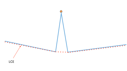
Figure 3: The LCE cannot capture global behavior for non-convex functions.

We now turn to a precise statement of this lemma and its proof:

Lemma 5.1 (Discretization).

. Let $(X,v,\sigma)$ be a RDF on $X=\mathcal{Z}^{d}\cap\mathcal{K}$ such that $v,\sigma$ are non-negative, moreover, for all $x\in X,v(x)-(8d^{2}+1)\sigma(x)\geq 0$. Assume further that there exists a convex function $F:{\mathbb{R}}^{d}\mapsto{\mathbb{R}}$ such that for all $x\in X$, $F(x)\in[v(x)-\sigma(x),v(x)+\sigma(x)]$. Let $\mathcal{K}^{\prime}=\mathcal{C}_{\mathcal{K}}$ be the enclosing bounding box for $\mathcal{K}$ such that $\mathbb{B}_{2^{4d^{2}}}(0)\subseteq\frac{4}{d^{2}}\mathcal{K}^{\prime}\subseteq\mathcal{K}\subseteq\mathcal{K}^{\prime}$ . Define $F_{\textsf{LCE}}=\textsf{LCE}(X,v,\sigma):\mathcal{K}^{\prime}\to{\mathbb{R}}$ as in Definition 4.4.

Then there exists a value $r=2^{3d^{2}}$ such that for every $y\in\frac{1}{4}\mathcal{K}$ with $\mathbb{B}_{r}(y)\subseteq\mathcal{K}$, there exists a point $y^{\prime}\in\mathbb{B}_{r}(y)$ with $F_{\textsf{LCE}}(y^{\prime})\geq\frac{1}{2}F(y)$.

5.1 Proof intuition in one dimension

The discretization lemma is the main technical challenge of our result, and as such we first give intuition for the proof for one dimension, for readability purposes only, and for the special case that the input DRF is actually a deterministic function (i.e. all variances are zero, and $v(x_{i})=F(x_{i})$ for a convex function $F$. The full proof is deferred to the appendix.

Proof.

Please refer to Figure 4 for an illustration.

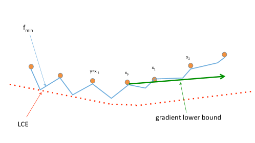
Figure 4: Discretization lemma in 1-d

Assume w.l.o.g. that $y\in\mathcal{Z}$, otherwise take the nearest point. Assume w.l.o.g that $f^{\prime}(y)>0$, and thus all points $x>y$ have value larger than $F(y)$. Consider the discrete points $\{y=x_{-1},x_{0},x_{1},....,\}$, and the value of $\tilde{f}_{\min}$ on these integer points, which by definition has to be equal to $F$, and thus larger than $F(y)$.

Since $F$ is increasing in the positive direction, we have that $\tilde{f}_{\min}(x_{0})\leq\tilde{f}_{\min}(x_{1})$, and by the definition of $\tilde{f}_{\min}$, the gradient from $x_{0}$ to $x_{1}$, implies that

$$\forall z\geq x_{1},\ \tilde{f}_{\min}(z)\geq\tilde{f}_{\min}(x_{0})$$

In the open interval $[x_{2},\infty)$, the value of the LCE is by definition a convex combination of values $\tilde{f}_{\min}(x)$ only for points in the range $x\in[x_{1},\infty)$. Thus, the function $F_{\textsf{LCE}}$ obtains a value larger than $\tilde{f}_{\min}(x_{1})\geq F(y)$ on all points within this range, which is within a distance of two from $y$. ∎

The proof of the Discretization Lemma requires the following lemmas:

Lemma 5.2 (Convex cover).

For every $k\in\mathbb{N}^{*}$, $r\in{\mathbb{R}}^{*}$, if $k$ convex sets $\mathcal{S}_{1},...,\mathcal{S}_{k}$ covers a ball in ${\mathbb{R}}^{d}$ of radius $r$, then there exists a set $\mathcal{S}_{i}$ that contains a ball of radius $\frac{r}{kd^{d}}$.

Proof of Lemma 5.2.

Consider the maximum volume contained Ellipsoid $\mathcal{E}_{i}$ of $\mathcal{S}_{i}\cap\mathbb{B}_{r}(0)$, we know that the volume of $\mathcal{E}_{i}$ is at least $1/d^{d}$ the volume of $\mathcal{S}_{i}\cap\mathbb{B}_{r}(0)$. Now, since $\mathcal{S}_{1},...,\mathcal{S}_{k}$ covers $\mathbb{B}_{r}(0)$, there exists a set $\mathcal{S}_{i}\cap\mathbb{B}_{r}(0)$ of volume at least $1/k$ fraction of the volume of $\mathbb{B}_{r}(0)$. Which implies that $\mathcal{E}_{i}$ has volume at least $1/(kd^{d})$ of $\mathbb{B}_{r}(0)$, note that $\mathcal{E}_{i}\subseteq\mathbb{B}_{r}(0)$, therefore, it contains a ball of radius $\frac{r}{kd^{d}}$. ∎

Lemma 5.3 (Approximation of polytope with integer points).

Suppose a polytope $\mathcal{P}_{o}=\mathop{\mbox{\rm conv}}\{v_{1},...,v_{d+1}\}\subseteq{\mathbb{R}}^{d}$ contains $\mathbb{B}_{4d^{8}}(0)$, then there exists $d+1$ integer points $g_{1},...,g_{d+1}\in\frac{2}{d^{2}}\mathcal{P}_{o}$ such that:

1. Let $(\lambda_{1},...,\lambda_{d+1})\in\Delta^{d+1}$ be the coefficient such that $\sum_{i}\lambda_{i}v_{i}=0$, then there exists $(\lambda_{1}^{\prime},...,\lambda_{d+1}^{\prime})\in\Delta^{d+1}$ such that $\sum_{i}\lambda_{i}^{\prime}g_{i}=0$. Moreover, $\frac{1}{2}\lambda_{i}^{\prime}\leq\lambda_{i}\leq 2\lambda_{i}^{\prime}$

2. For every $i\in[d+1]$, there exists $\{\lambda^{i}_{j}\in\Delta^{d+1}\}$ such that $\lambda_{i}^{i}\geq\frac{1}{2d^{2}}$ and

   $$g_{i}=\lambda^{i}_{i}v_{i}+\sum_{j\not=i}\lambda_{j}^{i}g_{j}$$

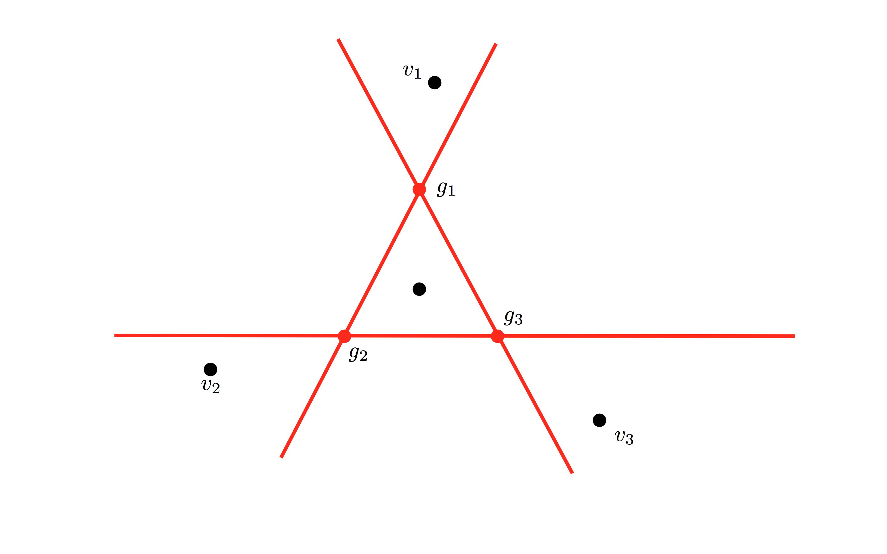
Figure 5: Approximation Lemma

Proof of Lemma 5.3.

Property 1:

Let $u_{i}=\frac{1}{d^{2}}v_{i}$. For every $i\in[n]$, since $\mathbb{B}_{4d^{8}}(0)\subseteq\mathop{\mbox{\rm conv}}\{v_{1},...,v_{d+1}\}$, it holds that

$$\mathbb{B}_{d}\left(u_{i}\right)\subseteq\mathop{\mbox{\rm conv}}\{v_{1},...,v_{d+1}\}$$

Therefore, we can find integer points around $u_{i}$ in $\mathop{\mbox{\rm conv}}\{v_{1},...,v_{d+1}\}$. Now, let $g_{i}$ be the closest integer point to $u_{i}$, which has distance at most $d$ to $u_{i}$, i.e. $\|g_{i}-u_{i}\|_{2}\leq d$. Observe that

$$\mathbb{B}_{d^{6}}\left(0\right)\subseteq\mathop{\mbox{\rm conv}}\{2u_{1},...,2u_{d+1}\}$$

Which implies that for every $i\in[d+1]$, $\mathbb{B}_{d^{6}/2}\left(u_{i}\right)\subseteq\mathop{\mbox{\rm conv}}\{2u_{1},...,2u_{d+1}\}$. Therefore, $g_{i}\in\mathop{\mbox{\rm conv}}\{2u_{1},...,2u_{d+1}\}=\frac{2}{d^{2}}\mathcal{P}_{o}$

Now we want to show that $0\in\mathop{\mbox{\rm conv}}\{g_{1},...,g_{d+1}\}$.

Consider a function $f:\mathop{\mbox{\rm conv}}\{u_{1},u_{2},...,u_{d+1}\}\to{\mathbb{R}}^{d}$ defined as: for $x=\sum_{i}\lambda_{i}^{\prime}u_{i}$ where $(\lambda_{1}^{\prime},\lambda_{2}^{\prime},...,\lambda_{d+1}^{\prime})\in\Delta^{d+1}$:

$$f(x)=\sum_{i}\lambda_{i}^{\prime}g_{i}$$

Observe that

$$\|f(x)-x\|_{2}=\left\|\sum_{i=1}^{d+1}\lambda_{i}^{\prime}\left(u_{i}-g_{i}\right)\right\|_{2}\leq d$$

Notice that for $x_{1},x_{2}\in\mathop{\mbox{\rm conv}}\{u_{1},u_{2},...,u_{d+1}\}$,

$$f\left(\frac{x_{1}+x_{2}}{2}\right)=\frac{f(x_{1})+f(x_{2})}{2}$$

Which implies that $f$ is a linear transformation. Moreover, $\mathbb{B}_{d^{2}}(0)\subseteq\mathop{\mbox{\rm conv}}\{u_{1},u_{2},...,u_{d+1}\}$. Therefore, $f(\mathbb{B}_{d^{2}}(0))=\cup_{x\in\mathbb{B}_{d^{2}}(0)}\{f(x)\}$ is a convex set, since a linear transformation preserves convexity.

Now, we want to show that $0\in f(\mathbb{B}_{d^{2}}(0))$. Suppose on the contrary $0\notin f(\mathbb{B}_{d^{2}}(0))$, then we know there is a separating hyperplane going through $0$ that separates $0$ and $f(\mathbb{B}_{d^{2}}(0))$. Which implies that there is a point $g^{\prime}\in\partial\mathbb{B}_{d^{2}}(0)$ such that

$$\textsf{dist}(g^{\prime},f(\mathbb{B}_{d^{2}}(0)))=\min_{x\in f(\mathbb{B}_{d^{2}}(0))}\|x-g^{\prime}\|\geq d^{2}$$

In particular, since $f(g^{\prime})\in f(\mathbb{B}_{d^{2}}(0))$, the above equality implies $\textsf{dist}(g^{\prime},f(g^{\prime}))\geq d^{2}$, in contradiction to $\|f(x)-x\|_{2}\leq d$. Therefore, $0\in f(\mathbb{B}_{d^{2}}(0))\subseteq\mathop{\mbox{\rm conv}}\{g_{1},...,g_{d}\}$.

We proceed to argue about the coefficients. Denote $g_{i}=u_{i}+b_{i}$, and by the above $\|b_{i}\|_{2}\leq d$. By symmetry it suffices to show that $\frac{1}{2}\lambda_{1}^{\prime}\leq\lambda_{1}\leq 2\lambda_{1}^{\prime}$.

Let $\{\lambda^{\prime}_{i}\}\in\Delta^{d+1}$ be such that $\sum_{i}\lambda_{i}^{\prime}g_{i}=\sum_{i}\lambda_{i}^{\prime}(u_{i}+b_{i})=0$. Then

$$\sum_{i}\lambda_{i}^{\prime}u_{i}=-\sum_{i}\lambda_{i}^{\prime}b_{i}$$

Since $\|b_{i}\|_{2}\leq d$, by the triangle inequality it holds that $\|\sum_{i}\lambda_{i}^{\prime}b_{i}\|_{2}\leq d$, which implies

$$\ \left\|\sum_{i}\lambda_{i}^{\prime}u_{i}\right\|\leq d$$

Let $H$ be the hyperplane going through $u_{2},...,u_{d+1}$. Without lost of generality, we can apply a proper rotation (unitary transformation) to put $H=\{x_{1}=-a\}$ for some value $a>0$, where $x_{1}$ denotes the first axis.

Now, (after rotation) Define $b=(b_{1},...,b_{d})=\sum_{i}\lambda_{i}^{\prime}u_{i}$ and denote $u_{1}=(a_{1},...,a_{d})$. The point $b$ is a convex combination of $u_{1}$ and $c:=\frac{1}{1-\lambda_{1}^{\prime}}\sum_{j\geq 2}\lambda_{j}^{\prime}u_{j}$. In addition we know that $c_{1}=-a$. Thus, we can write $\lambda_{1}^{\prime}$ as:

$$\lambda_{1}^{\prime}=\frac{b_{1}-c_{1}}{(u_{1})_{1}-c_{1}}=\frac{b_{1}+a}{a_{1}+a}$$

On the other hand, by $\sum_{i}\lambda_{i}u_{i}=0$, we know that

$$\lambda_{1}=\frac{a}{a_{1}+a}$$

Note that $\|b\|_{2}\leq d$, which implies $|b_{1}|<d$. However, by assumption there is a ball centered at $0$ of radius $4d^{6}$ in $\mathop{\mbox{\rm conv}}\{u_{1},...,u_{d+1}\}$, which implies $a\geq 4d^{6}\geq 4|b_{1}|$.

Therefore $\frac{1}{2}\lambda_{1}^{\prime}\leq\lambda_{1}\leq 2\lambda_{1}^{\prime}$.

Property 2:

By symmetry, it suffices to show for $v_{1}$. there exists $\lambda_{1}^{1}\geq\frac{1}{2d^{2}}$ and $\lambda_{j}^{1}\geq 0(j=2,3,...,d+1)$, $\lambda_{1}^{1}+\sum_{j=2}^{d+1}\lambda_{j}^{1}=1$ such that

$$g_{1}=\lambda_{1}^{1}v_{1}+\sum_{j=2}^{d+1}\lambda_{j}^{1}g_{j}$$

Consider a function $f:\mathop{\mbox{\rm conv}}\{v_{1},u_{2},...,u_{d+1}\}\to{\mathbb{R}}^{d}$ defined as: for $x=\lambda^{\prime}v_{1}+\sum_{j=2}^{d+1}\lambda_{j}^{\prime}u_{j}$ where $(\lambda^{\prime},\lambda_{2}^{\prime},...,\lambda_{d+1}^{\prime})\in\Delta^{d+1}$:

$$f(x)=\lambda^{\prime}v_{i}+\sum_{j=2}^{d+1}\lambda_{j}^{\prime}g_{j}$$

Observe that

$$\|f(x)-x\|_{2}=\left\|\sum_{j=2}^{d+1}\lambda_{j}^{\prime}\left(u_{j}-g_{j}\right)\right\|_{2}\leq d$$

Notice that for $x_{1},x_{2}\in\mathop{\mbox{\rm conv}}\{v_{1},u_{2},...,u_{d+1}\}$,

$$f\left(\frac{x_{1}+x_{2}}{2}\right)=\frac{f(x_{1})+f(x_{2})}{2}$$

Which implies that $f$ is a linear transformation. Moreover, $\mathbb{B}_{d^{2}}(g_{1})\subseteq\mathbb{B}_{2d^{2}}\left(u_{1}\right)\subseteq\mathop{\mbox{\rm conv}}\{v_{1},u_{2},...,u_{d+1}\}$. Therefore, $f(\mathbb{B}_{d^{2}}(g_{1}))=\cup_{x\in\mathbb{B}_{d^{2}}(g_{1})}\{f(x)\}$ is a convex set, since a linear transformation preserves convexity.

Now, we want to show that $g_{1}\in f(\mathbb{B}_{d^{2}}(g_{1}))$. Suppose on the contrary $g_{1}\notin f(\mathbb{B}_{d^{2}}(g_{1}))$, then we know there is a separating hyperplane going through $g_{1}$ that separates $g_{1}$ and $f(\mathbb{B}_{d^{2}}(g_{1}))$. Which implies that there is a point $g^{\prime}\in\mathbb{B}_{d^{2}}(g_{1})$ such that

$$\textsf{dist}(g^{\prime},f(\mathbb{B}_{d^{2}}(g_{1})))=\min_{x\in f(\mathbb{B}_{d^{2}}(g_{1}))}\|x-g^{\prime}\|=d^{2}$$

In particular, since $f(g^{\prime})\in f(\mathbb{B}_{d^{2}}(g_{1}))$, the above equality implies $\textsf{dist}(g^{\prime},f(g^{\prime}))\geq d^{2}$, in contradiction to $\|f(x)-x\|_{2}\leq d$ for all $x\in\mathop{\mbox{\rm conv}}\{v_{1},u_{2},...,u_{d+1}\}$.

Therefore, there is a point $g\in\mathbb{B}_{d^{2}}(g_{1})$ such that $f(g)=g_{1}$, i.e. $g_{1}$ can be written as

$$g_{1}=\lambda^{\prime}v_{1}+\sum_{j=2}^{d+1}\lambda_{j}^{\prime}g_{j}\quad(\lambda^{\prime},\lambda_{2}^{\prime},...,\lambda_{d+1}^{\prime})\in\Delta^{d+1}$$

We proceed to give a bound on the coefficients. Since $g_{1}=f(g)$, we know that

$$g=\lambda^{\prime}v_{1}+\sum_{j=2}^{d+1}\lambda_{j}^{\prime}u_{j}$$

On the other hand, observe that (since $\sum_{j}\lambda_{j}u_{j}=0$ as defined in Property 1)

$$u_{1}=\frac{1}{d^{2}}v_{1}+\left(1-\frac{1}{d^{2}}\right)\sum_{j=1}^{d+1}\lambda_{j}u_{j}$$

By $\|g-u_{1}\|_{2}\leq 2d^{2}$, using the same method as Property 1 we can obtain: $\lambda^{\prime}\geq\frac{1}{2d^{2}}$

Which completes the proof.

∎

Now we can prove the discretization Lemma. The proof goes by the following steps:

1. First, suppose the Lemma does not hold, then we can find a large hypercube that is contained inside $\mathcal{K}^{\prime}$ and has entirely small LCE compared to the value of the point $y$.

2. We proceed to identify the points whose $\tilde{f}_{min}$ value is associated with the LCE of the large hypercube, these $\tilde{f}_{min}$ have small values (compare to $F(y)$) and span a large region.

3. We find a simplex of $d+1$ points that span a large region in which the same holds, i.e. $\tilde{f}_{\min}$ value compared to $v(y)$.

4. Using the approximation Lemma, we find an inner simplex of $d+1$ discrete points inside the previous simplex. These discrete points all have $\tilde{f}_{\min}$ value larger than $f(y)$ by the fact that they are inside the first large region.

5. We use the definition of $\tilde{f}_{\min}$ to show that one of the vertices of the outer simplex has value of $\tilde{f}_{\min}$ larger than $f(y)$, in contradiction to the previous observations.

Proof of Lemma 5.1.

Step 1:

Consider a point $y\in P$ with $\mathbb{B}_{r}(y)\in\mathcal{K}$. By convexity of $F$, there is a hyperplane $H$ going $y$ such that on one side of the hyperplane, all the points have larger or equal $F$ value than $F(y)$. Therefore, there exists a point $y^{\prime}$, a cube $\mathcal{Q}_{r^{\prime}}(y^{\prime})\subset\mathbb{B}_{r}(y)$ centered at $y^{\prime}$ with radius $r^{\prime}=\frac{r}{2\sqrt{d}}$ such that for all integer points $z\in\mathcal{Q}_{r^{\prime}}(y^{\prime})$, $F(z)\geq F(y)$. Let $v_{1},...,v_{2^{d}}$ be the vertex of this cube.

If there exists $i\in[2^{d}]$ such that $F_{\textsf{LCE}}(v_{i})\geq\frac{1}{2}F(y)$, then we already conclude the proof. Therefore, we can assume that for all $i\in[2^{d}]$, $F_{\textsf{LCE}}(v_{i})<\frac{1}{2}F(y)$. Step 2:

By the definition of $F_{\textsf{LCE}}$, we know that for every $i\in[2^{d}]$, there exists $p_{i,1},....,p_{i,m}\in\mathcal{K}^{\prime}$ such that $v_{i}=\sum_{j}\lambda_{i,j}p_{i,j},(\lambda_{i,1},...,\lambda_{i,m})\in\Delta^{m}$ with

$$F_{\textsf{LCE}}(v_{i})=\sum\lambda_{i,j}\tilde{F}_{\min}(p_{i,j})<\frac{1}{2}F(y)$$

Moreover, by Carath odory’s theorem , we can make $m=d+1$.

Now we get a set of $(d+1)2^{d}$ many points $P_{o}=\{p_{i,j}\}_{i\in[2^{d}],j\in[d+1]}$. Consider a size $d+1$ subset $J=\{p_{i_{1},j_{1}},...,p_{i_{d+1},j_{d+1}}\}$ of $P_{o}$, define convex set

$$S_{J}=\left\{x\in\mathcal{Q}_{r^{\prime}}(y^{\prime})\mid\exists(\lambda_{1},...,\lambda_{d+1})\in\Delta^{d+1}:x=\sum_{s}\lambda_{s}p_{i_{s},j_{s}},\sum_{s}\lambda_{s}\tilde{F}_{\min}(p_{i_{s},j_{s}})<\frac{1}{2}F(y)\right\}$$

We claim that

$$\mathop{\bigcup}_{J\subseteq P_{0},|J|=d+1}S_{J}=\mathcal{Q}_{r^{\prime}}(y^{\prime})$$

This is because for every $x\in\mathcal{Q}_{r^{\prime}}(y^{\prime})$, there exists $v_{i_{1}},...,v_{i_{d+1}}$ and $\lambda_{1},...,\lambda_{d+1}\in\Delta^{d+1}$ such that

$$\sum_{s\in[d+1]}\lambda_{s}v_{i_{s}}=x$$

Moreover, for each $v_{i}$, $v_{i}=\sum_{j}\lambda_{i,j}p_{i,j}$. Therefore:

$$x=\sum_{s\in[d+1]}\lambda_{s}\left(\sum_{j}\lambda_{i_{s},j}p_{i_{s},j}\right)$$

On the other hand, $\sum_{s\in[d+1]}\lambda_{s}\left(\sum_{j}\lambda_{i_{s},j}\tilde{F}_{\min}(p_{i_{s},j})\right)<\frac{1}{2}F(y)$. By Carath odory’s theorem, we can make the sum only contains $d+1$ such $p_{i_{s},j}$, which proves the claim.

Step 3:

By lemma 5.2, we know that there exists $J^{*}$ such that $S_{J^{*}}$ contains a ball $\mathbb{B}_{r^{\prime\prime}}(y^{\prime\prime})$ inside $Q_{r^{\prime}}(y^{\prime})$ of radius $r^{\prime\prime}=\frac{r^{\prime}}{2\sqrt{d}kd^{d}}$ where $k={(d+1)2^{d}\choose d+1}\leq 2^{2d^{2}}$ and $y^{\prime\prime}$ is an integer point.

For simplicity, we denote $J^{*}=\{p_{1},...,p_{d+1}\}$. By the definition of $S_{J^{*}}$, there exists $(\lambda_{1}^{\prime\prime},...,\lambda_{d+1}^{\prime\prime})\in\Delta^{d+1}$ such that

1. $$\sum_{i}\lambda_{i}^{\prime\prime}p_{i}=y^{\prime\prime}$$

2. $$\sum_{i}\lambda_{i}^{\prime\prime}\tilde{F}_{\min}(p_{i})<\frac{1}{2}F(y)$$

Step 4:Let $P=\mathop{\mbox{\rm conv}}\{p_{1},...,p_{d+1}\}$ with center $y^{\prime\prime}$. The above argument implies that $\mathbb{B}_{r^{\prime\prime}}(y^{\prime\prime})\subseteq\mathop{\mbox{\rm conv}}\{p_{1},...,p_{d+1}\}$, when $r^{\prime\prime}=\frac{r^{\prime}}{2\sqrt{d}kd^{d}}\geq\frac{r}{(2d)^{2d^{2}}}\geq 4d^{8}$. By lemma 5.3, there exists integer points $g_{1},...,g_{d+1}\in\frac{2}{d^{2}}P$ (where $\frac{2}{d^{2}}P$ denotes shrink $P$ of factor $\frac{2}{d^{2}}$ according to center $y^{\prime\prime}$) with

1. $y^{\prime\prime}\in\mathop{\mbox{\rm conv}}\{g_{1},...,g_{d+1}\}$

2. For every $i\in[d+1]$, there exists $\{\lambda^{i}_{j}\in\Delta^{d+1}\}$ such that $\lambda_{i}^{i}\geq\frac{1}{2d^{2}}$ and

   $$g_{i}=\lambda^{i}_{i}p_{i}+\sum_{j\not=i}\lambda_{j}^{i}g_{j}$$

The conditions of the lemma assert that $\frac{2}{d^{2}}\mathcal{K}^{\prime}\subseteq\frac{1}{2}\mathcal{K}$, by $y^{\prime\prime}\in\frac{1}{2}\mathcal{K},P\subseteq\mathcal{K}^{\prime}$, we know that $\frac{2}{d^{2}}P\subseteq\mathcal{K}$. This implies that $g_{i}\in\mathcal{Z}^{d}\cap\mathcal{K}$, over which the RDF is defined, and we have values $v(g_{i})$ and $\sigma(g_{i})$ to construct $\tilde{F}_{\min}$.

Step 5:

By the fact that $g_{i}=\lambda_{i}p_{i}^{i}+\sum_{j\not=i}\lambda_{j}^{i}g_{j}$ and the definition of $\tilde{F}_{\min}$, we know that

$$\tilde{F}_{\min}(p_{i})\geq\frac{1}{\lambda_{i}^{i}}\left(v(g_{i})-\sigma(g_{i})-\sum_{j\not=i}\lambda_{j}^{i}[v(g_{j})+\sigma(g_{j})]\right)$$

Let us write $y^{\prime\prime}=\sum_{i}\lambda_{i}^{\prime}g_{i}:(\lambda_{1}^{\prime},...,\lambda_{d+1}^{\prime})\in\Delta^{d+1}$. By the fact that $p_{i}=\frac{1}{\lambda_{i}^{i}}(g_{i}-\sum_{j\not=i}\lambda_{j}^{i}g_{j})$ We can calculate:

$$y^{\prime\prime}=\sum_{i}\lambda_{i}^{\prime\prime}p_{i},\quad\text{where }\frac{\lambda_{i}^{\prime\prime}}{\lambda_{i}^{i}}-\sum_{j\not=i}\frac{\lambda^{\prime\prime}_{j}\lambda_{i}^{j}}{\lambda_{j}^{j}}=\lambda^{\prime}_{i}$$

From Lemma 5.3 we also obtain that $\lambda_{i}^{\prime\prime}\leq 2\lambda_{i}^{\prime}$.

Moreover, for the interpolation:

$$\sum_{i}\lambda_{i}^{\prime\prime}\tilde{F}_{\min}(p_{i})$$

$$\geq \sum_{i}\frac{\lambda_{i}^{\prime\prime}}{\lambda_{i}^{i}}\left(v(g_{i})-\sigma(g_{i})-\sum_{j\not=i}\lambda_{j}^{i}[v(g_{j})+\sigma(g_{j})]\right)$$

$$= \sum_{i}\frac{\lambda_{i}^{\prime\prime}}{\lambda_{i}^{i}}\left(v(g_{i})+\sigma(g_{i})-\sum_{j\not=i}\lambda_{j}^{i}[v(g_{j})+\sigma(g_{j})]\right)-2\sum_{i}\frac{\lambda_{i}^{\prime\prime}}{\lambda_{i}^{i}}\sigma(g_{i})$$

$$= \sum_{i}\left(\left[\frac{\lambda_{i}^{\prime\prime}}{\lambda_{i}^{i}}-\sum_{j\not=i}\frac{\lambda_{j}^{\prime\prime}\lambda_{i}^{j}}{\lambda_{j}^{j}}\right][v(g_{i})+\sigma(g_{i})]\right)-2\sum_{i}\frac{\lambda_{i}^{\prime\prime}}{\lambda_{i}^{i}}\sigma(g_{i})$$

$$= \sum_{i}\lambda_{i}^{\prime}[v(g_{i})+\sigma(g_{i})]-2\sum_{i}\frac{\lambda_{i}^{\prime\prime}}{\lambda_{i}^{i}}\sigma(g_{i})$$

$$\geq \sum_{i}\lambda_{i}^{\prime}[v(g_{i})+\sigma(g_{i})]-4d^{2}\sum_{i}\lambda_{i}^{\prime}\sigma(g_{i})\quad\quad\mbox{ since $\lambda_{i}^{i}\geq\frac{1}{d^{2}}$,$\lambda_{i}^{\prime\prime}\leq 2\lambda_{i}^{\prime}$ }$$

$$= \sum_{i}\lambda_{i}^{\prime}[v(g_{i})-(4d^{2}-1)\sigma(g_{i})]$$

By assumption, since $g_{i}$ is a integer point, we get $v(g_{i})-(8d^{2}+1)\sigma(g_{i})\geq 0$

$$v(g_{i})-(4d^{2}-1)\sigma(g_{i}) \geq v(g_{i})+\sigma(g_{i})-4d^{2}\sigma(g_{i})$$

$$\geq F(g_{i})-4d^{2}\sigma(g_{i})\quad\quad\text{ since by definition }v(g_{i})+\sigma(g_{i})\geq F(g_{i})$$

$$\geq F(g_{i})-\frac{v(g_{i})-\sigma(g_{i})}{2}\quad\quad\text{ since }(8d^{2}+1)\sigma(g_{i})\leq v(g_{i})$$

$$\geq \frac{1}{2}F(g_{i})\quad\quad\text{ since by definition }v(g_{i})-\sigma(g_{i})\leq F(g_{i})$$

Note that by the convexity of $F$, $\sum_{i}\lambda_{i}^{\prime}F(g_{i})\geq F(y^{\prime\prime})\geq F(y)$ (last inequality is due to our choice of $y^{\prime\prime}$). Thus,

$$\sum_{i}\lambda_{i}^{\prime\prime}\tilde{F}_{\min}(p_{i})\geq\sum_{i}\frac{1}{2}\lambda_{i}^{\prime}F(g_{i})\geq\frac{1}{2}F(y)$$

By contradiction we complete the proof.

∎

6 Algorithm and statement of results

6.1 Algorithm statement and parameter setting

1. $\delta>0$ - an upper bound on the failure probability of the algorithm

2. The desired regret bound $\ell=\left(2^{d^{4}}(\log T)^{2d}\log\frac{1}{\delta}\right)\sqrt{T}$

3. resolution of the grid: $\alpha=2^{3d^{2}}\log^{3}T\geq\gamma\beta^{2}\sqrt{d}$.

4. Scaling factor $\beta=4096d^{4}\log T$.

5. Extension ratio: $\gamma=2048d^{4}\log T$.

6. Blow up factor $\eta=8d^{2}+1$.

7. Upper bound on the number of epoch $\tau\leq 8d^{2}\log T$.

Algorithm 3 Bandit Ellipsoid

1:  Input: A convex set $\mathcal{K}\subseteq{\mathbb{R}}^{d}$, $\mathcal{A}$: a high-probability low regret bandit algorithm on discrete set of points

2:  Initialize: Epoch $\tau=0$, epoch set $\Gamma_{\tau}=\emptyset$, $\mathcal{K}_{\tau}=\mathcal{K}$, Grid $\operatorname{grid}_{\tau}=\operatorname{grid}(\beta\mathcal{K}_{\tau}\cap\mathcal{K})$

3:  for $t=1$ to $T$ do

4:     Apply the low-regret algorithm on current grid:

$$(p_{t},v_{t},\sigma_{t})\leftarrow\mathcal{A}(\operatorname{grid}_{\tau},\{p_{i},x_{i},f_{i}(x_{i})\mid i\in\Gamma_{\tau}\})$$

where $p_{t},v_{t},\sigma_{t}$ are defined as in section 2.1.

5:     Play a point $x_{t}\in\operatorname{grid}_{\tau}$ from distribution $p_{t}(x_{t})$, observe value $f_{t}(x_{t})$. Set $\Gamma_{\tau}=\Gamma_{\tau}\cup\{t\}$.

6:     (Shift): Shift $v_{t}$ by a constant so that $\min_{x\in\operatorname{grid}_{\tau}}\{v_{t}(x)-\eta\sigma_{t}(x)\}=0$, for simplicity we just keep the same notation for the new $v_{t}$. Moreover, we can shift $F^{\tau}=\sum_{j\in\Gamma_{\tau}}f_{j}$ by the same constant and assume that adversary presents us the (shifted) $f_{j}$. For simplicity we also keep the same notation for the new $F^{\tau}$.

7:     Compute $F_{\textsf{LCE}}^{\tau}=\text{FitLCE}(\beta\mathcal{K}_{\tau}\cap\mathcal{K},[\operatorname{grid}_{\tau},v_{\tau},\sigma_{\tau}])$.

8:     if  $\forall x\in\mathcal{K}_{\tau},\exists j\leq\tau,F_{\textsf{LCE}}^{j}(x)>\frac{\ell}{4}$ then

9:        RESTART (goto Initialize)

10:     end if

11:     if (DecideMove)  $\exists\tilde{x}_{\tau}\in\frac{\mathcal{K}_{\tau}}{\beta}$ such that $F_{\textsf{LCE}}^{\tau}(\tilde{x}_{\tau})\geq\ell$  then

12:        $\mathcal{K}_{\tau+1}=\text{ShrinkSet}(\mathcal{K}_{\tau},\tilde{x}_{\tau},F_{\textsf{LCE}}^{\tau},\operatorname{grid}_{\tau},\{v_{t},\sigma_{t}\})$

13:        Set $\Gamma_{\tau+1}=\emptyset$, $\operatorname{grid}_{\tau+1}=\text{grid}(\beta\mathcal{K}_{\tau+1}\cap\mathcal{K},\alpha)$, $\tau=\tau+1$.

14:     end if

15:  end for

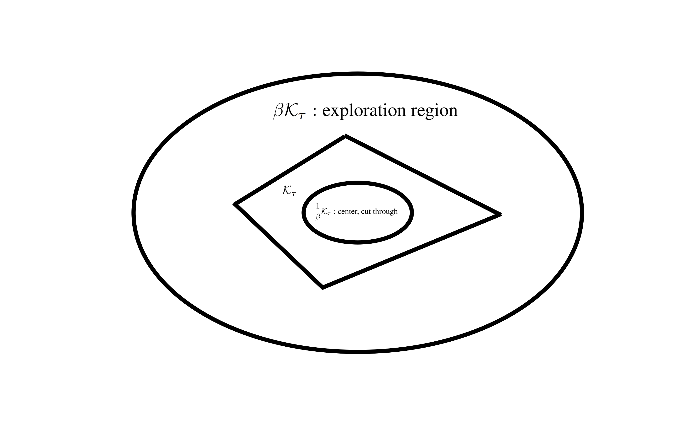
Figure 6: Depiction of the algorithm

This algorithm calls upon two subroutines, FitLCE which was defined in section 4, and ShrinkSet which we now define.

Algorithm 4 ShrinkSet

1:  Input: Convex set $\mathcal{K}_{\tau}$, convex function $F_{\textsf{LCE}}^{\tau}$, point $\tilde{x}_{\tau}\in\mathcal{K}_{\tau}$, Grid $\operatorname{grid}_{\tau}$, value estimation $v_{t}$ and variance estimation $\sigma_{t}$.

2:  Compute a separation hyperplane $H_{\tau}^{\prime}$ through $\tilde{x}_{\tau}$ between $\tilde{x}_{\tau}$ and $\{y\mid F_{\textsf{LCE}}^{\tau}(y)<\ell\}$. Assume $H_{\tau}^{\prime}=\{x\mid\langle h_{\tau},x\rangle=w_{\tau}\}$ and $\{y\mid F_{\textsf{LCE}}^{\tau}(y)<\ell\}\subseteq\{y\mid\langle h_{\tau},x\rangle\leq w_{\tau}\}$

3:  Let $x_{\tau}$ be the center of the MVEE ${\mathcal{E}}_{\tau}$ of $\mathcal{K}_{\tau}$.

4:  (Amplify Distance). Let $H_{\tau}=\{x\mid\langle h_{\tau},x\rangle=z_{\tau}\}$ for some $z_{\tau}\geq 0$ such that the following holds:

1. $\{y\mid F_{\textsf{LCE}}^{\tau}(y)<\ell\}\subseteq\{y\mid\langle h_{\tau},y\rangle\leq z_{\tau}\}$

2. $\textsf{dist}(x_{\tau},H_{\tau})=2\textsf{dist}(x_{\tau},H_{\tau}^{\prime})$.

3. $\langle h_{\tau},x_{\tau}\rangle\leq z_{\tau}$.

5:  Return $\mathcal{K}_{\tau+1}=\left(\mathcal{K}_{\tau}\cap\{y\mid\langle h_{\tau},y\rangle\leq z_{\tau}\}\right)$

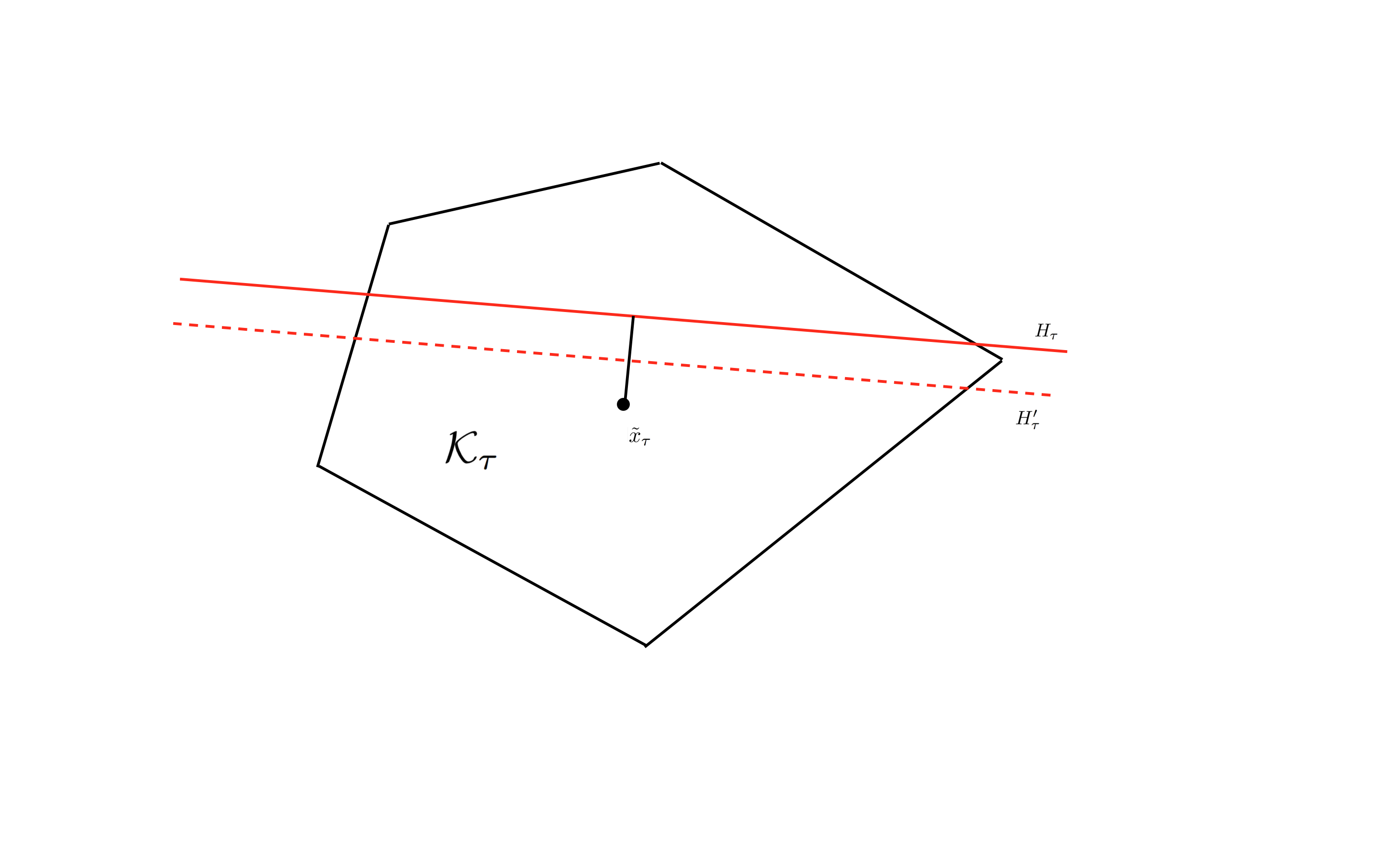
Figure 7: Depiction of the ShrinkSet procedure

6.2 Statement of main theorem

Theorem 6.1 (Main, full algorithm).

Suppose for all time $t$ in all epoch $\tau$, $\mathcal{A}$ outputs $v_{t}$ and $\sigma_{t}$ such that for all $x\in\operatorname{grid}_{\tau}$, $\left(\sum_{j\in\Gamma_{\tau},j\leq t}f_{j}(x)\right)\in[v_{t}(x)-\sigma_{t}(x),v_{t}(x)+\sigma_{t}(x)]$. Moreover, $\mathcal{A}$ achieves a value

$$v_{\tau}(\mathcal{A})=\sum_{j\in\Gamma_{\tau},j\leq t}f_{j}(x_{j})\leq\min_{x\in\operatorname{grid}_{\tau}}\left\{v_{t}(x)-\eta\sigma_{t}(x)\right\}+\frac{\ell}{1024d^{3}\log T}$$

then Algorithm 3 satisfies

$$\sum_{t}f_{t}(x_{t})-\min_{x^{*}}\sum_{t}f_{t}(x^{*})\leq\ell$$

Corollary 6.1 (Exp3.P.).

Algorithm 3 with $\mathcal{A}$ being Exp3.P satisfies the condition in Theorem 6.1 with probability $1-\delta$ for

$$\ell=\left(2^{d^{4}}(\log T)^{2d}\log\frac{1}{\delta}\right)\sqrt{T}$$

6.3 Running time

Our algorithm runs in time $O\left((\log T)^{\mathop{\mbox{\rm poly}}(d)}\right)$, which follows from Theorem 4.1 and the running time of Exp3.P on $K\leq(2d\alpha)^{d}$ Experts

6.4 Analysis sketch

Before going to the details, we briefly discuss the steps of the proof.

Step 1: In the algorithm, we shift the input function so that the player can achieve a value $\leq\sqrt{T}$. Therefore, to get the regret bound, we can just focus on the minimal value of $\sum_{t}f_{t}$.

Step 2: We follow the standard Ellipsoid argument, maintaining a shrinking set, which at epoch $\tau$ is denoted $\mathcal{K}_{\tau}$. We show the volume of this set decreases by a factor of at least $1-\frac{1}{d}$, and hence the number of epochs between iterative RESTART operations can be bounded by $O(d^{2}\log T)$ (when the diameter of $\mathcal{K}_{\tau}$ along one direction decreases below $\frac{1}{\sqrt{T}}$, we do not need to further discretizate along that direction).

Step 3: We will show that inside each epoch $\tau$, for every $x\in\mathcal{K}_{\tau}$, $\sum_{t:t\text{ in epoch }\tau}f_{t}(x)$ is lower bounded by $-\frac{2\ell}{\gamma}$ for $\ell\approx\sqrt{T},\gamma\geq 1$. For point $x$ outside the $\mathcal{K}_{\tau}$, $\sum_{t:t\text{ in epoch }\tau}f_{t}(x)$ is lower bounded by $-\frac{2\ell}{\gamma}\gamma(x,\mathcal{K}_{\tau})$.

Step 4: We will show that when one epoch $\tau$ ends, for every point $x$ cut off by the separation hyperplane, $\sum_{t:t\text{ in epoch }\tau}f_{t}(x)$ is lower bounded by $\frac{\ell}{2}\gamma(x,\mathcal{K}_{\tau})$

Step 5: Putting the result of 3, 4 together, we know that for a point outside the current set $\mathcal{K}_{\tau}$, it must be cut off by a separation hyperplane at some epoch $j\leq\tau$. Moreover, we can find such $j$ with $\gamma(x,\mathcal{K}_{j})\geq\frac{\gamma(x,\mathcal{K}_{\tau})}{d}$. Which implies that

$$\sum_{t}f_{t}(x)=\sum_{t:t\text{ in epoch }1,2,...,j-1,j+1,...,\tau}f_{t}(x)+\sum_{t:t\text{ in epoch }j}f_{t}(x)\geq-\frac{2\tau\ell}{\gamma}\gamma(x,\mathcal{K}_{\tau})+\frac{\ell\gamma(x,\mathcal{K}_{\tau})}{2d}\approx\sqrt{T}$$

By our choice of $\gamma\geq 8d\tau$. Therefore, when the adversary wants to move the optimal outside the current set $\mathcal{K}_{\tau}$, the player has zero regret. Moreover, by the result of 3, inside current set $\mathcal{K}_{\tau}$, the regret is bounded by $\tau\frac{2\ell}{\gamma}\approx\sqrt{T}$.
The crucial steps in our proof are Step 3 and Step 4. Here we briefly discuss about the intuition to prove the two steps.

Intuition of Step 3: For $x\in\mathcal{K}_{\tau}$, we use the grid property (Property of grid, 2.1) to find a grid $x_{g}$ point such that $x_{c}=x_{g}+\gamma(x_{g}-x)$ is close to the center of $\mathcal{K}_{\tau}$. Since $x_{g}$ is a grid point, by shifting we know that

$$\sum_{t:t\text{ in epoch }\tau}f_{t}(x_{g})\geq 0$$

Therefore, if $\sum_{t:t\text{ in epoch }\tau}f_{t}(x)<-\frac{2\ell}{\gamma}$, by convexity of $f_{t}$, we know that $\sum_{t:t\text{ in epoch }\tau}f_{t}(x_{c})\geq 2\ell$. Now, apply discretization Lemma 5.1, we know that there is a point $x^{\prime}_{c}$ near $x_{c}$ such that $F_{\textsf{LCE}}^{\tau}(x_{c}^{\prime})\geq\ell$, by our DecideMove condition, the epoch $\tau$ should end. Same argument can be applied to $x\notin\mathcal{K}_{\tau}$.

Intuition of Step 4: We use the fact that the algorithm does not RESTART, therefore, according to our condition, there is a point $x_{0}\in\mathcal{K}_{\tau}$ with $F_{\textsf{LCE}}^{\tau}(x_{0})\leq\frac{\ell}{4}$. Observe that the separation hyperplane of our algorithm separates $x_{0}$ with points whose $F_{\textsf{LCE}}^{\tau}\geq\ell$. Using the convexity of $F_{\textsf{LCE}}$, we can show that $F_{\textsf{LCE}}^{\tau}(x)\geq\frac{\ell}{2}\gamma(x,\mathcal{K}_{\tau})$. Apply the fact that $F_{\textsf{LCE}}^{\tau}$ is a lower bound of $\sum_{t:t\text{ in epoch }\tau}f_{t}$ we can conclude $\sum_{t:t\text{ in epoch }\tau}f_{t}(x)\geq\frac{\ell}{2}\gamma(x,\mathcal{K}_{\tau})$.

Notice that here we use the convexity of $F_{\textsf{LCE}}$, and also the fact that it is a lower bound on $F$ (standard convex regression is not a lower bound on $F$, see section 3 for further discussion on this issue).

Now we can present the proof for general dimension $d$

To prove the main theorem we need the following lemma, starting from the following corollary of Lemma 5.1:

Corollary 6.2.

(1). For every epoch $\tau$, $\forall x\in\beta\mathcal{K}_{\tau}\cap\mathcal{K}$,

$$F_{\textsf{LCE}}^{\tau}(x)\leq F^{\tau}(x)=\sum_{i\in\Gamma_{\tau}}f_{i}(x)$$

.
(2). For every epoch $\tau$, let $x_{\tau}$ be the center of the MVEE of $\mathcal{K}_{\tau}$, then $F^{\tau}(x)=\sum_{i\in\Gamma}f_{i}(x)\leq 2\ell$.

Proof.

(1) is just due to the definition of LCE. (2) is due to the Geometry Lemma on $F^{\tau}$: for every $x\in\frac{\mathcal{K}}{2\beta}$, there exists $x^{\prime}\in\left(x+\frac{\mathcal{K}_{\tau}}{2\beta}\right)\subseteq\frac{\mathcal{K}_{\tau}}{\beta}$ such that $F_{\textsf{LCE}}^{\tau}(x^{\prime})\geq\frac{1}{2}F^{\tau}(x)$ ∎

Lemma 6.1 (During an epoch).

During every epoch $\tau$ the following holds:

$$F^{\tau}(x)\geq{\left\{\begin{array}[]{ll}{-\frac{2\ell}{\gamma}}&{x\in\mathcal{K}\cap\mathcal{K}_{\tau}}\\ \\ {-\frac{2\gamma(x,\mathcal{K}_{\tau})\ell}{\gamma}}&{x\in\mathcal{K}\cap\mathcal{K}_{\tau}^{c}}\end{array}\right.}$$

Lemma 6.2 (Number of epoch).

There are at most $8d^{2}\log T$ many epochs before RESTART.

Proof of 6.2.

Let $\mathcal{E}_{\tau}$ be the minimal volume enclosing Ellipsoid of $\mathcal{K}_{\tau}$, we will show that

$$\mbox{\rm vol}(\mathcal{E}_{\tau+1})\leq\left(1-\frac{1}{8d}\right)\mbox{\rm vol}(\mathcal{E}_{\tau})$$

First note that $\mathcal{K}_{\tau+1}=\mathcal{K}_{\tau}\cap\mathcal{H}$ for some half space $\mathcal{H}$ corresponding to the separating hyperplane going through $\frac{1}{\beta}\mathcal{E}_{\tau}$, therefore, $\mathcal{K}_{\tau+1}\subset\mathcal{E}_{\tau}\cap\mathcal{H}$.

Let $\mathcal{E}_{\tau+1}^{\prime}$ be the minimal volume enclosing Ellipsoid of $\mathcal{E}_{\tau}\cap\mathcal{H}$, we know that

$$\mbox{\rm vol}(\mathcal{E}_{\tau})\leq\mbox{\rm vol}(\mathcal{E}_{\tau+1}^{\prime})$$

Without lose of generality, we can assume that $\mathcal{E}_{\tau}$ is centered at 0. Let $A$ be a linear operator on $\mathbb{R}^{d}$ such that $A(\mathcal{E}_{\tau})$ is the unit ball $\mathbb{B}_{1}(0)$, observe that

$$\frac{\mbox{\rm vol}(\mathcal{E}_{\tau+1}^{\prime})}{\mbox{\rm vol}(\mathcal{E}_{\tau})}=\frac{\mbox{\rm vol}(A\mathcal{E}_{\tau+1}^{\prime})}{\mbox{\rm vol}(A\mathcal{E}_{\tau})}$$

Since $A\mathcal{E}_{\tau+1}^{\prime}$ is the MVEE of $A\mathcal{E}_{\tau}\cap A\mathcal{H}$, where $A\mathcal{H}$ is the halfspace corresponding to the separating hyperplane going through $\mathbb{B}_{\frac{1}{\beta}}(0)$. Without lose of generality, we can assume that $\mathcal{H}=\{x\in{\mathbb{R}}^{d}\mid x_{1}\geq a\}$ for some $a$ such that $|a|\leq\frac{1}{\beta}\leq\frac{1}{d^{2}}$.

Observe that

$$A\mathcal{E}_{\tau}\cap A\mathcal{H}\subseteq\left\{x\in{\mathbb{R}}^{d}\left|\right.\frac{(x_{1}-\frac{1}{4d})^{2}}{\left(1-\frac{1}{4d}\right)^{2}}+\frac{x_{2}^{2}}{1+\frac{1}{12d^{2}}}+...+\frac{x_{d}^{2}}{1+\frac{1}{12d^{2}}}\leq 1\right\}=\mathcal{E}$$

Therefore,

$$\mbox{\rm vol}(A\mathcal{E}_{\tau+1}^{\prime})\leq\mbox{\rm vol}(\mathcal{E})\leq 1-\frac{1}{8d}.$$

Now, observe that the algorithm will not cut through one eigenvector of the MVEE of $\mathcal{K}_{\tau}$ if its length is smaller than $\frac{1}{\sqrt{T}}$, and the algorithm will stop when all its eigenvectors have length smaller than $\frac{1}{\sqrt{T}}$. Therefore, the algorithm will make at most

$$d\log_{1-\frac{1}{8d}}\left(\frac{1}{\sqrt{T}}\right)=8d^{2}\log T$$

many epochs. ∎

Lemma 6.3 (Beginning of each epoch).

For every $\tau\geq 0$:

$$\sum_{i=0}^{\tau-1}F^{i}(x)\geq{\left\{\begin{array}[]{ll}{-\tau\frac{2\ell}{\gamma}}&{x\in\mathcal{K}\cap\mathcal{K}_{\tau}}\\ \\ {\frac{\gamma(x,\mathcal{K}_{\tau})\ell}{64d}}&{x\in\mathcal{K}\cap\mathcal{K}_{\tau}^{c}}\end{array}\right.}$$

Lemma 6.4 (Restart).

(After shifting) If $\mathcal{A}$ obtains a value $v_{j}(\mathcal{A})=\sum_{t\in\Gamma_{j}}f_{t}(x_{t})\leq\frac{\ell}{1024d^{3}\log T}$ for each epoch $j$, then when the algorithm RESTART, $\mbox{Regret}=0$.

6.5 Proof of main theorem

Now we can prove the regret bound assuming all the lemmas above, whose proof we defer to the next section.

Proof of Theorem 6.1.

Using Lemma 6.4, we can only consider epochs between two RESTART. Now, for epoch $\tau$, we know that for $x\in\mathcal{K}\cap\mathcal{K}_{\tau}^{c}$,

$$\sum_{i\in\Gamma_{0}\cup...\cup\Gamma_{\tau-1}}f_{i}(x)\geq\frac{\gamma(x,\mathcal{K}_{\tau})\ell}{64d}$$

$$\sum_{i\in\Gamma_{\tau}}f_{i}(x)\geq-\frac{2\gamma(x,\mathcal{K}_{\tau})\ell}{\gamma}$$

Therefore, for $x\in\mathcal{K}\cap\mathcal{K}_{\tau}^{c}$

$$\sum_{i\in\Gamma_{0}\cup...\cup\Gamma_{\tau}}f_{i}(x)\geq{\gamma(x,\mathcal{K}_{\tau})\ell}\left(\frac{1}{64d}-\frac{2}{\gamma}\right)\geq 0$$

By our choice of $\gamma=2048d^{4}\log T$.

In the same manner, we know that for $x\in\mathcal{K}\cap\mathcal{K}_{\tau}$,

$$\sum_{i\in\Gamma_{0}\cup...\cup\Gamma_{\tau}}f_{i}(x)\geq-\frac{2(\tau+1)\ell}{\gamma}\geq-\frac{\ell}{2}$$

By $\tau\leq 8d^{2}\log T$.

Which implies that for every $x\in\mathcal{K}$, $\sum_{i\in\Gamma_{0}\cup...\cup\Gamma_{\tau}}f_{i}(x)\geq-\frac{\ell}{2}$.

Denote by $v_{j}(\mathcal{A})=\sum_{i\in\Gamma_{j},i\leq t}f_{j}(x_{j})$ the overall loss incurred by the algorithm in epoch $j$ before time $t$. The low-regret algorithm $\mathcal{A}$ guarantees that in each epoch:

$$v_{j}(\mathcal{A}) = \sum_{i\in\Gamma_{\tau},i\leq t}f_{i}(x_{i})$$

$$\leq \min_{x\in\operatorname{grid}_{\tau}}\left\{v_{t}(x)-\eta\sigma_{t}(x)\right\}+\frac{\ell}{1024d^{3}\log T}$$

$$\leq \frac{\ell}{1024d^{3}\log T}\quad\quad\mbox{ by shifting }\min_{x\in\operatorname{grid}_{\tau}}\left\{v_{t}(x)-\eta\sigma_{t}(x)\right\}=0$$

Thus $\mathcal{A}$ obtains over all epochs a total value of at most

$$\sum_{0\leq j\leq\tau}\frac{\ell}{1024d^{3}\log T}=(\tau+1)\times\frac{\ell}{1024d^{3}\log T}\leq\frac{\ell}{2}.$$

Therefore,

$$\mbox{Regret}=\sum_{0\leq j\leq\tau}v_{j}(\mathcal{A})-\sum_{i\in\Gamma_{0}\cup...\cup\Gamma_{\tau}}f_{i}(x^{*})\leq\ell$$

∎

7 Analysis and proof of main lemmas

7.1 Proof of Lemma 6.1

Proof of 6.1.

Part 1:

Consider any $x\in\mathcal{K}_{\tau}$. By Lemma 2.1 part 1, we know that there exists $x_{g}\in\operatorname{grid}_{\tau}$ such that $x_{c}=x_{g}+\gamma(x-x_{g})\in\frac{\mathcal{K}_{\tau}}{2\beta}$. Any convex function $f$ satisfies for any two points $y,z$ that $f(\gamma x+(1-\gamma)y)\leq\gamma f(x)+(1-\gamma)f(y)$. Applying this to the convex function $F^{\tau}$ over the line on which the points $x,x_{c},x_{g}$ reside and observe $\gamma=\frac{\|x_{c}-x_{g}\|_{2}}{\|x_{g}-x\|_{2}}$, we have

$${F^{\tau}(x_{c})-F^{\tau}(x_{g})}\geq\frac{||x_{c}-x_{g}||_{2}}{||x_{g}-x||_{2}}({F^{\tau}(x_{g})-F^{\tau}(x)})=\gamma({F^{\tau}(x_{g})-F^{\tau}(x)})$$

Since $x_{g}\in\operatorname{grid}$ and we shifted all losses on the grid to be nonnegative, $F^{\tau}(x_{g})\geq 0$. Thus, we can simplify the above to:

$$F^{\tau}(x_{c})\geq-\gamma F^{\tau}(x)$$

Since the epoch is ongoing, the conditions of DecideMove are not yet satisfied, and hence $\forall x^{\prime}\in\frac{1}{\beta}\mathcal{K}_{\tau},\ F_{\textsf{LCE}}^{\tau}(x^{\prime})\leq\ell$. By (2) of Lemma 6.2 for all points $x^{\prime\prime}$ in $\frac{1}{2\beta}\mathcal{K}_{\tau}$ it holds that $F^{\tau}(x^{\prime\prime})\leq 2\ell$, in particular $F^{\tau}(x_{c})\leq 2\ell$. The above simplifies to

$$F^{\tau}(x)\geq-\frac{1}{\gamma}F^{\tau}(x_{c})\geq-\frac{2\ell}{\gamma}$$

Part 2:

For $x\in\mathcal{K}_{\tau}^{c}\cap\mathcal{K}$ By Lemma 2.1 part 2, we know that there exists $x_{g}\in\operatorname{grid}_{\tau}$ such that $x_{c}=x_{g}+\frac{\gamma}{\gamma(x,\mathcal{K}_{\tau})}(x-x_{g})\in\frac{\mathcal{K}_{\tau}}{\beta^{2}}$. Now, by the convexity of $F^{\tau}$, we know that

$${F^{\tau}(x_{c})-F^{\tau}(x_{g})}{}\geq\frac{||x_{c}-x_{g}||_{2}}{||x_{g}-x||_{2}}\left(F^{\tau}(x_{g})-F^{\tau}(x)\right)=\frac{\gamma}{\gamma(x,\mathcal{K}_{\tau})}\left(F^{\tau}(x_{g})-F^{\tau}(x)\right)$$

Since $x_{g}\in\operatorname{grid}$ and we shifted all losses on the grid to be nonnegative, $F^{\tau}(x_{g})\geq 0$. Thus, we can simplify the above to:

$${F^{\tau}(x_{c})}\geq-\frac{\gamma}{\gamma(x,\mathcal{K}_{\tau})}F^{\tau}(x)$$

Since the epoch is ongoing, the conditions of DecideMove are not yet satisfied, and hence $\forall x^{\prime}\in\frac{1}{\beta}\mathcal{K}_{\tau},\ F_{\textsf{LCE}}^{\tau}(x^{\prime})\leq\ell$. By (2) of Lemma 6.2 for all points $x^{\prime\prime}$ in $\frac{1}{2\beta}\mathcal{K}_{\tau}$ it holds that $F^{\tau}(x^{\prime\prime})\leq 2\ell$, in particular $F^{\tau}(x_{c})\leq 2\ell$. The above simplifies to

$$F^{\tau}(x)\geq-\frac{\gamma(x,\mathcal{K}_{\tau})}{\gamma}F^{\tau}(x_{c})\geq-\frac{2\gamma(x,\mathcal{K}_{\tau})\ell}{\gamma}$$

∎

7.2 Proof of Lemma 6.3

Proof of Lemma 6.3.

Part 1: For every $x\in\mathcal{K}\cap\mathcal{K}_{\tau}$, since $K_{\tau}\subseteq\mathcal{K}_{\tau-1}\subseteq...\subseteq\mathcal{K}_{0}=\mathcal{K}$, we have $x\in\mathcal{K}_{j}$ for every $0\leq j\leq\tau$. Therefore, by Lemma 6.1 we get $F^{j}(x)\geq-\frac{2\ell}{\gamma}$. Summing over the epochs,

$$\sum_{i=0}^{\tau-1}F^{i}(x)\geq-\tau\frac{2\ell}{\gamma}$$

Part 2: Figure 8 illustrates the proof.

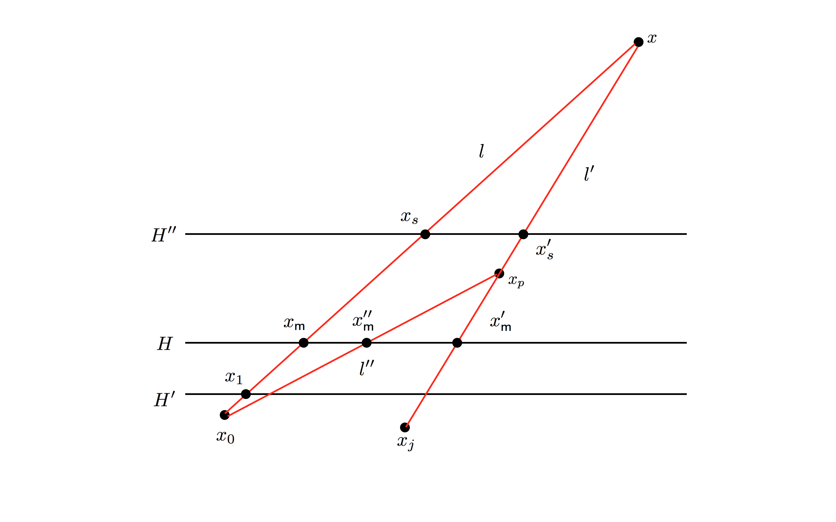
Figure 8: geometric intution for the proof

For every $x\in\mathcal{K}\cap\mathcal{K}_{\tau}^{c}$, since the Algorithm does not RESTART, therefore, there must be a point $x_{0}\in\mathcal{K}_{\tau}$ such that

$$\forall\tau^{\prime}\leq\tau,F_{\textsf{LCE}}^{\tau^{\prime}}(x_{0})\leq\frac{\ell}{4}$$ (2)

Let $l$ be the line segment between $x$ and $x_{0}$. Since $x\notin\mathcal{K}_{\tau}$, the line $l$ intersects $\mathcal{K}_{\tau}$, and denote $x_{\textsf{m}}$ be the intersection point between $l$ and $\mathcal{K}_{\tau}$: $\{x_{\textsf{m}}\}=l\cap\mathcal{K}_{\tau}$. The corresponding boundary of $\mathcal{K}_{\tau}$ was constructed in an epoch $j\leq\tau$, and a hyperplane which separates the $\ell$-level set of $\mathcal{K}_{j}$, namely $H=\{x_{\textsf{m}}\mid\langle h_{j},x_{\textsf{m}}\rangle=z_{j}\})$ (See ShrinkSet for definition of $h_{j},z_{j}$) such that $H\cap l=\{x_{\textsf{m}}\}$.

Now, by the definition of Minkowski Distance, we know that (Since Minkowski Distance is the distance ratio to $\frac{1}{d}{\mathcal{E}}_{\tau}$ where ${\mathcal{E}}_{\tau}$ is the MVEE of $\mathcal{K}_{\tau}$, $\frac{1}{d}{\mathcal{E}}_{\tau}$ can be $1/d$ smaller than $\mathcal{K}_{\tau}$, and $x_{\textsf{m}}$ is the intersection point to $\mathcal{K}_{\tau}$)

$$\frac{||x-x_{\textsf{m}}||_{2}}{||x_{\textsf{m}}-x_{0}||_{2}}\geq\frac{\gamma(x,\mathcal{K}_{\tau})-1}{2d}$$

We know that (by the convexity of $F_{\textsf{LCE}}^{j}$)

$$\frac{F_{\textsf{LCE}}^{j}(x)-F_{\textsf{LCE}}^{j}(x_{\textsf{m}})}{F_{\textsf{LCE}}^{j}(x_{\textsf{m}})-F_{\textsf{LCE}}^{j}(x_{0})}\geq\frac{||x-x_{\textsf{m}}||_{2}}{||x_{\textsf{m}}-x_{0}||_{2}}\geq\frac{\gamma(x,\mathcal{K}_{\tau})-1}{2d}$$

where the denominator is non-negative, by equation (2), $F_{\textsf{LCE}}^{j}(x_{0})\leq\frac{\ell}{4}$, and by the definition of $H$ (separation hyperplane of the $\ell$-level-set of $F_{\textsf{LCE}}^{j}$), $F_{\textsf{LCE}}^{j}(x_{\textsf{m}})\geq\ell$. This implies

$$F_{\textsf{LCE}}^{j}(x)\geq\frac{(\gamma(x,\mathcal{K}_{\tau})-1)\cdot\frac{3}{4}\ell}{2d}+\ell\geq\frac{\gamma(x,\mathcal{K}_{\tau})\ell}{4d}$$

We consider the following two cases: (a). $x\in\beta\mathcal{K}_{j}$, (b). $x\notin\beta\mathcal{K}_{j}$.

case (a): $x\in\beta\mathcal{K}_{j}$

The LCE is a lower bound of the original function only for $x$ in the LCE fitting domain, here LCE = $F_{\textsf{LCE}}^{j}$, original function $F^{j}:\beta\mathcal{K}_{j}\cap\mathcal{K}\to{\mathbb{R}}$, so it is only true for $x\in\beta\mathcal{K}_{j}\cap\mathcal{K}$. Now, by (1) in Lemma 6.2, we know that $F^{j}(x)\geq F_{\textsf{LCE}}^{j}(x)\geq\frac{\gamma(x,\mathcal{K}_{\tau})\ell}{4d}$.

For other epoch $i<\tau$, we can apply Lemma 6.1 and get $F^{i}(x)\geq-\frac{2\gamma(x,\mathcal{K}_{i})\ell}{\gamma}$. Since the set $\mathcal{K}_{\tau}\subseteq\mathcal{K}_{\tau-1}\subseteq...\subseteq\mathcal{K}_{0}$, By John’s theorem, we can conclude that $\gamma(x,\mathcal{K}_{i})\leq 2d\gamma(x,\mathcal{K}_{\tau})$

which implies

$$\sum_{i=0}^{\tau-1}F^{i}(x) \geq \sum_{i\not=j}F^{i}(x)+F^{j}(x)$$

$$\geq \frac{\gamma(x,\mathcal{K}_{\tau})\ell}{4d}-\tau\times\frac{4d\gamma(x,\mathcal{K}_{\tau})\ell}{\gamma}\geq\frac{\gamma(x,\mathcal{K}_{\tau})\ell}{32d}$$

by our choice of parameters $\tau\leq 8d^{2}\log T$ and $\gamma=2048d^{4}\log T$.

case (b): $x\notin\beta\mathcal{K}_{j}$, $x\in\mathcal{K}$

This part of the proof consists of three steps. First, We find a point $x_{j}$ in center of $\mathcal{K}_{j}$ that has low $F^{j}$ value. Then we find a point $x_{p}$ inside $\beta\mathcal{K}_{j}$, on the line between $x_{j}$ and $x$, with large $F_{\textsf{LCE}}^{j}$ value, which implies by lemma 6.2 it has large $F^{j}$ value. Finally, we use both $x_{0},x_{p}$ to deduce the large value of $F^{j}(x)$.

Step1: Let $x_{j}$ be the center of MVEE ${\mathcal{E}}_{j}$ of $\mathcal{K}_{j}$. By (2) in Lemma 6.2, we know that $F^{j}(x_{j})\leq 2\ell$.

Step 2: Define $H^{\prime}=\{y\mid\langle y,h_{j}\rangle=w_{j}\}$ to be the hyperplane parallel to $H$ such that $\textsf{dist}(x_{j},H^{\prime})=\frac{1}{2}\textsf{dist}(x_{j},H)$, and $H^{\prime\prime}=\{y\mid\langle y,h_{j}\rangle=u_{j}\}$ to be the hyperplane parallel to $H$ such that $\textsf{dist}(x_{0},H^{\prime\prime})=9\textsf{dist}(x_{0},H)$.

We can assume $\langle x_{0},h_{j}\rangle<w_{j}$ ($x_{0},H$ are in different side of $H^{\prime}$), since we know that $F_{\textsf{LCE}}^{j}(x_{0})\leq\frac{\ell}{4}$ by definition, and the hyperplane $H^{\prime}$ separates such that all points with $\langle x_{0},h_{j}\rangle\geq w_{j}$ (See ShrinkSet for definition of $H$, $H^{\prime}$) have value $F_{\textsf{LCE}}^{j}(x)\geq\ell$.

Note $\langle x_{0},h_{j}\rangle<w_{j}$ implies $\textsf{dist}(x_{0},H)\geq\frac{1}{2}\textsf{dist}(x_{j},H)=\textsf{dist}(H,H^{\prime})$ , which implies that

$$\textsf{dist}(x_{j},H^{\prime\prime})\geq\textsf{dist}(H,H^{\prime\prime})=8\textsf{dist}(x_{0},H)\geq 4\textsf{dist}(x_{j},H).$$

Now, let $x_{s}=l\cap H^{\prime\prime}$ be the intersection point between $H^{\prime\prime}$ and $l$, we can get: $x_{s}=x_{\textsf{m}}+8(x_{\textsf{m}}-x_{0})$. Since $x_{0},x_{\textsf{m}}\in\mathcal{K}_{j}$ , we can obtain $x_{s}\in\frac{\beta}{2}\mathcal{K}_{j}$ by our choice of $\beta\geq 64d^{2}$. Let $x_{s}^{\prime}=l^{\prime}\cap H^{\prime\prime}$ be the intersection point of $H^{\prime\prime}$ and the line segment $l^{\prime}$ of $x$ and $x_{j}$. Let $x_{1}$ be the intersection point of $H^{\prime}$ and $l$: $\{x_{1}\}=H^{\prime}\cap l$.

Consider the plane defined by $x_{0},x_{j},x$. Define $x_{p}$ to be the intersecting point of the ray shooting from $x_{s}$ towards the interval $[x,x_{j}]$, that is parallel to the line from $x_{1}$ to $x_{j}$.

Note that $\|x_{s}-x_{p}\|\leq\|x_{1}-x_{j}\|$, we have:

$$x_{p}=x_{s}+(x_{p}-x_{s})=x_{s}+(x_{j}-x_{1})\frac{||x_{s}-x_{p}||}{||x_{1}-x_{j}||}$$

We know that $x_{1},x_{j}\in\mathcal{K}_{j}$, $x_{s}\in\frac{\beta}{2}\mathcal{K}_{j}$, therefore, $x_{s}+(x_{j}-x_{1})\frac{||x_{s}-x_{p}||}{||x_{1}-x_{j}||}\in\beta\mathcal{K}_{j}$, which means $x_{p}\in\beta\mathcal{K}_{j}$. Moreover, we know that $||x_{s}^{\prime}-x_{p}||_{2}\leq||x_{p}-x_{\textsf{m}}^{\prime}||_{2}$ due to the fact that $||x_{s}^{\prime}-x_{p}||_{2}\leq||x_{\textsf{m}}^{\prime}-x_{j}||_{2}\leq\frac{1}{2}\|x_{\textsf{m}}^{\prime}-x_{s}^{\prime}\|_{2}$ (last inequality by $\textsf{dist}(x_{j},H^{\prime\prime})\geq 4\textsf{dist}(x_{j},H)$).

We also note that $||x_{s}^{\prime}-x_{p}||_{2}\leq||x_{p}-x_{\textsf{m}}^{\prime}||_{2}$ implies

$$\textsf{dist}(x_{p},H)\geq\frac{1}{2}\textsf{dist}(x_{s}^{\prime},H).$$

Now, let $l^{\prime\prime}$ be the line segment between $x_{p}$ and $x_{0}$, let $x_{\textsf{m}}^{\prime\prime}$ be the intersection point of $H$ and $l^{\prime\prime}$: $H\cap l^{\prime\prime}=\{x_{\textsf{m}}^{\prime\prime}\}$.

Consider the value of $F^{j}(x_{p})$, by (1) in Lemma 6.2 and $x_{p}\in\beta\mathcal{K}_{j}$, we know that $F^{j}(x_{p})\geq F_{\textsf{LCE}}^{j}(x_{p})$. By the convexity of $F_{\textsf{LCE}}^{j}$, we obtain:

$$\frac{F_{\textsf{LCE}}^{j}(x_{p})-F_{\textsf{LCE}}^{j}(x_{\textsf{m}}^{\prime\prime})}{F_{\textsf{LCE}}^{j}(x_{\textsf{m}}^{\prime\prime})-F_{\textsf{LCE}}^{j}(x_{0})} \geq \frac{||x_{p}-x_{\textsf{m}}^{\prime\prime}||_{2}}{||x_{\textsf{m}}^{\prime\prime}-x_{0}||_{2}}$$

$$= \frac{\textsf{dist}(x_{p},H)}{\textsf{dist}(x_{0},H)}$$

$$\geq \frac{\frac{1}{2}\textsf{dist}(x_{s}^{\prime},H)}{\textsf{dist}(x_{0},H)}$$

$$= \frac{\frac{1}{2}\textsf{dist}(H^{\prime\prime},H)}{\textsf{dist}(x_{0},H)}=4$$

Note that $F_{\textsf{LCE}}^{j}(x_{\textsf{m}}^{\prime\prime})\geq\ell$, $F_{\textsf{LCE}}^{j}(x_{0})\leq\frac{\ell}{4}$, therefore, $F_{\textsf{LCE}}^{j}(x_{p})\geq 3\ell$. Which implies $F^{j}(x_{p})\geq F_{\textsf{LCE}}^{j}(x_{p})\geq 3\ell$.

Step 3:

Due to $x\notin\beta\mathcal{K}_{j}$ and $x_{m}\in\mathcal{K}_{j}$, by our choice of $x_{s}$ and $\beta$, we know that $||x-x_{\textsf{m}}||_{2}\geq 8||x_{s}-x_{\textsf{m}}||_{2}$.

We ready to bound the value of $F^{j}(x)$: By the convexity of $F^{j}$, we have:

$$\frac{F^{j}(x)-F^{j}(x_{p})}{F^{j}(x_{p})-F^{j}(x_{j})} \geq \frac{||x-x_{p}||_{2}}{||x_{p}-x_{j}||_{2}}=\frac{||x-x_{s}||_{2}}{||x_{s}-x_{1}||_{2}}\quad\quad\text{triangle similarity}$$

$$= \frac{||x-x_{\textsf{m}}||_{2}-||x_{s}-x_{\textsf{m}}||_{2}}{||x_{\textsf{m}}-x_{1}||_{2}+||x_{s}-x_{\textsf{m}}||_{2}}$$

$$\geq \frac{||x-x_{\textsf{m}}||_{2}}{2||x_{s}-x_{\textsf{m}}||_{2}}\quad\quad\mbox{ by $||x_{s}-x_{\textsf{m}}||_{2}\geq 8||x_{\textsf{m}}-x_{1}||$}$$

$$\geq \frac{||x-x_{\textsf{m}}||_{2}}{||x_{\textsf{m}}-x_{0}||_{2}}\times\frac{||x_{\textsf{m}}-x_{0}||_{2}}{2||x_{s}-x_{\textsf{m}}||_{2}}$$

$$\geq \frac{\gamma(x,\mathcal{K}_{\tau})-1}{32d}$$

The last inequality is due to $\frac{||x_{\textsf{m}}-x_{0}||_{2}}{||x_{s}-x_{\textsf{m}}||_{2}}=\frac{1}{8}$ and $\frac{||x-x_{\textsf{m}}||_{2}}{||x_{\textsf{m}}-x_{0}||_{2}}\geq\frac{\gamma(x,\mathcal{K}_{\tau})-1}{2d}$

Putting together, we obtain (by $F^{j}(x_{j})\leq 2\ell$):

$$F^{j}(x)\geq\frac{\gamma(x,\mathcal{K}_{\tau})-1}{32d}\left(F^{j}(x_{p})-F^{j}(x_{j})\right)\geq\frac{\gamma(x,\mathcal{K}_{\tau})-1}{32d}$$

Same as case (a) , we can sum over rest epoch to obtain:

$$\sum_{i=0}^{\tau-1}F^{i}(x)\geq\frac{(\gamma(x,\mathcal{K}_{\tau})-1)\ell}{32d}-\tau\times\frac{4d\gamma(x,\mathcal{K}_{\tau})\ell}{\gamma}\geq\frac{\gamma(x,\mathcal{K}_{\tau})\ell}{64d}$$

by our choice of parameters $\tau\leq 8d^{2}\log T$ and $\gamma=2048d^{4}\log T$.

∎

7.3 Proof of Lemma 6.4

Proof of Lemma 6.4.

Suppose algorithm RESTART at epoch $\tau$, then $\sum_{j\leq\tau}v_{j}(\mathcal{A})\leq\frac{\ell}{128d}$. Therefore, we just need to show that for every $x\in\mathcal{K}$,

$$\sum_{i\in\Gamma_{0}\cup...\cup\Gamma_{\tau}}f_{i}(x)\geq\frac{\ell}{128d}$$

.

(a). Since the algorithm RESTART, by the RESTART condition, for every $x\in\mathcal{K}_{\tau}$, we know that $\exists j\leq\tau$ such that $F^{j}(x)=\sum_{i\in\Gamma_{j}}f_{i}(x)\geq F_{\textsf{LCE}}^{j}(x)>\frac{\ell}{4}$. Using Lemma 6.1, we know that for every $j^{\prime}\leq\tau,j^{\prime}\not=j$: $F^{j^{\prime}}(x)=\sum_{i\in\Gamma_{j^{\prime}}}f_{i}(x)\geq-\frac{2\ell}{\gamma}$.

Which implies that

$$\sum_{i\in\Gamma_{0}\cup...\cup\Gamma_{\tau}}f_{i}(x)\geq\frac{\ell}{4}-\tau\frac{2\ell}{\gamma}\geq\frac{\ell}{8}$$

(b). For every $x\notin\mathcal{K}_{\tau}$, by Lemma 6.3, we know that

$$\sum_{i\in\Gamma_{0}\cup...\cup\Gamma_{\tau-1}}f_{i}(x)\geq\frac{\gamma(x,\mathcal{K}_{\tau})\ell}{64d}$$

Moreover, by Lemma 6.1, we know that

$$\sum_{i\in\Gamma_{\tau}}f_{i}(x)\geq-\frac{2\gamma(x,\mathcal{K}_{\tau})\ell}{\gamma}$$

Putting together we have:

$$\sum_{i\in\Gamma_{0}\cup...\cup\Gamma_{\tau}}f_{i}(x)\geq\gamma(x,\mathcal{K}_{\tau})\left(\frac{\ell}{64d}-\frac{2\ell}{\gamma}\right)\geq\frac{\ell}{128d}$$

∎

8 The EXP3 algorithm

For completeness, we give in this section the definition of the EXP3.P algorithm of [5], in slight modification which allows for unknown time horizon and output of the variances.

Algorithm 5 Exp3.P

1:  Initial: $T=1$.

2:  Input: $K$ experts, unknown rounds. In round $t$ the cost function is given by $f_{t}$.

3:  Let $\gamma=\sqrt{\frac{K\ln K}{T}}$, $\alpha=\sqrt{\ln\left(\frac{KT}{\delta}\right)}$,

4:  for $j=1,...,K$ do

5:     set

$$w_{1}(j)=\exp\left(\eta\alpha\gamma\sqrt{\frac{T}{K}}\right)$$

6:  end for

7:  for $t=T,...,2T-1$ do

8:     for $j=1,...,K$ do

9:        

$$p_{t}(j)=(1-\gamma)\frac{w_{t}(j)}{\sum_{j^{\prime}}w_{t}(j^{\prime})}+\frac{\gamma}{K}$$

10:     end for

11:     pick $j_{t}$ at random according to $p_{t}(j)$, play expert $j_{t}$ and receive $f_{t}(j_{t})$

12:     for $j=1,...,K$ do

13:        Let

$$\hat{f}_{t}(j)=\left\{\begin{array}[]{ll}\frac{f_{t}(j)}{p_{t}(j)}&\mbox{if $j=j_{t}$};\\ 0&\mbox{otherwise}.\end{array}\right.$$

14:        And

$$\hat{g}_{t}(j)=\left\{\begin{array}[]{ll}\frac{1-f_{t}(j)}{p_{t}(j)}&\mbox{if $j=j_{t}$};\\ 0&\mbox{otherwise}.\end{array}\right.$$

15:     end for

16:     Update

$$w_{t+1}(j)=w_{t}(j)\exp\left(\frac{\gamma}{K}\left(\hat{g}_{t}(j)+\frac{\eta\alpha}{p_{t}(j)\sqrt{TK}}\right)\right)$$

17:     return  

$$v_{t}(j)=\sum_{i=1}^{t}\hat{f}_{i}(j)$$

and

$$\sigma_{t}(j)=\sum_{i=1}^{t}\frac{\alpha}{p_{i}(j)\sqrt{TK}}$$

18:  end for

19:  Set $T=2T$ and Goto 3.

9 Acknowledgements

We would like to thank Aleksander Madry for very helpful conversations during the early stages of this work.

References

- [1] Rediet Abebe. Counting regions in hyperplane arrangements. Harvard College Math Review, 5.
- [2] Jacob Abernethy, Elad Hazan, and Alexander Rakhlin. Competing in the dark: An efficient algorithm for bandit linear optimization. In COLT, pages 263–274, 2008.
- [3] Alekh Agarwal, Ofer Dekel, and Lin Xiao. Optimal algorithms for online convex optimization with multi-point bandit feedback. In COLT, pages 28–40, 2010.
- [4] Alekh Agarwal, Dean P. Foster, Daniel Hsu, Sham M. Kakade, and Alexander Rakhlin. Stochastic convex optimization with bandit feedback. SIAM Journal on Optimization, 23(1):213–240, 2013.
- [5] Peter Auer, Nicolò Cesa-Bianchi, Yoav Freund, and Robert E. Schapire. The nonstochastic multiarmed bandit problem. SIAM J. Comput., 32(1):48–77, January 2003.
- [6] Baruch Awerbuch and Robert Kleinberg. Online linear optimization and adaptive routing. J. Comput. Syst. Sci., 74(1):97–114, 2008.
- [7] Keith Ball. An elementary introduction to modern convex geometry. In Flavors of Geometry, pages 1–58. Univ. Press, 1997.
- [8] Sébastien Bubeck and Nicolo Cesa-Bianchi. Regret analysis of stochastic and nonstochastic multi-armed bandit problems. Foundations and Trends in Machine Learning, 5(1):1–122, 2012.
- [9] Sébastien Bubeck, Nicolò Cesa-Bianchi, and Sham M. Kakade. Towards minimax policies for online linear optimization with bandit feedback. Journal of Machine Learning Research - Proceedings Track, 23:41.1–41.14, 2012.
- [10] Sébastien Bubeck, Ofer Dekel, Tomer Koren, and Yuval Peres. Bandit convex optimization: \(\sqrt{T}\) regret in one dimension. In Proceedings of The 28th Conference on Learning Theory, COLT 2015, Paris, France, July 3-6, 2015, pages 266–278, 2015.
- [11] Sébastien Bubeck and Ronen Eldan. Multi-scale exploration of convex functions and bandit convex optimization. CoRR, abs/1507.06580, 2015.
- [12] Andrew R Conn, Katya Scheinberg, and Luis N Vicente. Introduction to Derivative-Free Optimization, volume 8. Society for Industrial and Applied Mathematics, 2009.
- [13] Varsha Dani, Thomas P. Hayes, and Sham Kakade. The price of bandit information for online optimization. In NIPS, 2007.
- [14] Ofer Dekel, Ronen Eldan, and Tomer Koren. Bandit smooth convex optimization: Improving the bias-variance tradeoff. In Advances in Neural Information Processing Systems 28: Annual Conference on Neural Information Processing Systems 2015, 2015.
- [15] Abraham Flaxman, Adam Tauman Kalai, and H. Brendan McMahan. Online convex optimization in the bandit setting: gradient descent without a gradient. In SODA, pages 385–394, 2005.
- [16] M. Grötschel, L. Lovász, and A. Schrijver. Geometric algorithms and combinatorial optimization. Algorithms and combinatorics. Springer-Verlag, 1993.
- [17] Elad Hazan. DRAFT: Introduction to online convex optimimization. Foundations and Trends in Machine Learning, XX(XX):1–168, 2015.
- [18] Elad Hazan and Zohar Karnin. Hard-margin active linear regression. In 31st International Conference on Machine Learning (ICML 2014), 2014.
- [19] Elad Hazan and Kfir Y. Levy. Bandit convex optimization: Towards tight bounds. In Advances in Neural Information Processing Systems 27: Annual Conference on Neural Information Processing Systems 2014, December 8-13 2014, Montreal, Quebec, Canada, pages 784–792, 2014.
- [20] F. John. Extremum Problems with Inequalities as Subsidiary Conditions. In K. O. Friedrichs, O. E. Neugebauer, and J. J. Stoker, editors, Studies and Essays: Courant Anniversary Volume, pages 187–204. Wiley-Interscience, New York, 1948.
- [21] Robert D Kleinberg. Nearly tight bounds for the continuum-armed bandit problem. In NIPS, volume 17, pages 697–704, 2004.
- [22] Eunji Lim and Peter W. Glynn. Consistency of multidimensional convex regression. Oper. Res., 60(1):196–208, January 2012.
- [23] Hariharan Narayanan and Alexander Rakhlin. Random walk approach to regret minimization. In Advances in Neural Information Processing Systems 23: 24th Annual Conference on Neural Information Processing Systems 2010. Proceedings of a meeting held 6-9 December 2010, Vancouver, British Columbia, Canada., pages 1777–1785, 2010.
- [24] Ankan Saha and Ambuj Tewari. Improved regret guarantees for online smooth convex optimization with bandit feedback. In AISTATS, pages 636–642, 2011.
- [25] Ohad Shamir. On the complexity of bandit and derivative-free stochastic convex optimization. In Conference on Learning Theory, pages 3–24, 2013.