Mixed and stabilized finite element methods for the obstacle problem

Abstract

We discretize the Lagrange multiplier formulation of the obstacle problem by mixed and stabilized finite element methods. A priori and a posteriori error estimates are derived and numerically verified.

65N30

1 Introduction

In its classical form, the obstacle problem is an archtype example of a variational inequality [35]. The problem corresponds to finding the equilibrium position of an elastic membrane constrained to lie above a rigid obstacle. Other examples of obstacle-type problems are found, e.g., in lubrication theory [40], in flows through porous media [22], in control theory [38] and in financial mathematics [18].

Discretization of the primal variational formulation of the obstacle problem by the finite element method has been extensively studied since the 1970’s. Error estimates for the membrane displacement in the $H^{1}$-norm have been obtained, e.g., by Falk [19], Mosco–Strang [36] and Brezzi–Hager–Raviart [10]. For an overview of the early progress on the subject and the respective references, see the monograph of Glowinski [23].

Instead of focusing on the primal formulation, we study an alternative variational formulation based on the method of Lagrange multipliers [2, 9, 11, 27]. The Lagrange multiplier formulation introduces an additional physically relevant unknown, the reaction force between the membrane and the obstacle, which in itself can be a useful tool—especially in the context of contact mechanics, cf. Hlaváček et al. [31] or, more recently, Wohlmuth [49]. Furthermore, the alternative formulation leads naturally to an effective solution strategy based on the semismooth Newton method [30, 46] and provides also a straightforward justification for the related Nitsche-type method that follows from the local elimination of the Lagrange multiplier in the stabilized discrete problem [44].

A priori error analysis for finite element methods based on a Lagrange multiplier formulation of the obstacle problem has been performed by Haslinger et al. [28], Weiss–Wohlmuth [48] and Schröder et al. [42, 3]. A posteriori error estimates were derived, e.g., in Bürg–Schröder [13] or Banz–Stephan [4] and, using a similar Lagrange multiplier formulation, in Veeser [47], Braess [6] and Gudi–Porwal [26].

The purpose of this paper is to readdress the Lagrange multiplier formulation of the obstacle problem. We consider two methods. The first is a mixed method in which the stability is achieved by adding bubble degrees of freedom to the displacement. The second approach is a residual-based stabilized method similar to the methods used successfully for the Stokes problem [32, 20]. The latter technique has been applied to variational inequalities arising from contact problems in Hild–Renard [29].

Until our recent article on the Stokes problem [45], error estimates on stabilized methods were always built upon the assumption that the exact solution is regular enough, with the additional regularity assumptions arising from the stabilizing terms. In [45], we realized that these extra regularity requirements can be dropped and only the loading term needs to be in $L^{2}$. In this work, we extend these ideas to variational inequalities. We emphasize that the improved error estimates can only be established if the discrete stability bound is proven in correct norms, i.e. in the norms of the continuous problem and not in mesh dependent norms as, for example, in Hild–Renard [29] where the authors need to assume that the solution to the Signorini problem is in $H^{s}$, with $s>3/2$.

We perform the analysis in a unified manner. First, we prove a stability result for the continuous problem in proper norms. This estimate becomes useful in deriving the a posteriori estimates. As for the discretizations, we start by proving stability with respect to a mesh dependent norm. This discrete stability result implies stability in the continuous norms and yields quasi optimal a priori estimates without additional regularity assumptions. For the stabilized methods, we use a technique first suggested by Gudi [25].

The stabilized formulation of the classical Babu$\check{\rm s}$ka’s method of Lagrange multipliers for approximating Dirichlet boundary conditions is known to be closely related to Nitsche’s method [37]. This connection has been used for the contact problem in Hild–Renard [29] and Chouly–Hild [16], and for the obstacle problem in [14]. We show that a similar relationship holds here as well and observe that for the lowest order method it leads to the penalty formulation.

We end the paper by reporting on extensive numerical computations.

2 Problem definition

Consider finding the equilibrium position $u=u(x,y)$ of an elastic, homogeneous membrane constrained to lie above an obstacle represented by $g=g(x,y)$. The membrane is loaded by a normal force $f=f(x,y)$ and its boundary is held fixed. The problem can be formulated as

(2.1) $$-\Delta u-f \geq 0 {\rm in}~{}\Omega,$$

$$u-g \geq 0 {\rm in}~{}\Omega,$$

$$(u-g)(\Delta u+f) =0 {\rm in}~{}\Omega,$$

$$u =0 {\rm on}~{}\partial\Omega,$$

where $\Omega\subset\mathbb{R}^{2}$ is a smooth bounded domain or a convex polygon, and where we assume that $g=0$ at $\partial\Omega$. Let $V=H^{1}_{0}(\Omega)$. The problem (2.1) can be recast as the following variational inequality: find $u\in\mathcal{V}$ such that

(2.2) $$\big{(}\nabla u,\nabla(v-u)\big{)}\geq(f,v-u)\quad\forall v\in\mathcal{V},$$

where

(2.3) $$\mathcal{V}=\{v\in V:v\geq g~{}{\rm a.e.~{}in}\ \Omega\}.$$

It is well known that, given $f\in L^{2}(\Omega)$ and $g\in H^{1}(\Omega)\cap C(\overline{\Omega})$, problem (2.2) admits a unique solution $u\in\mathcal{V}$, cf. Lions–Stampacchia [35], or Kinderlehrer–Stampacchia [34]. Given that the second derivatives of $u$ have a jump across the free boundary separating the contact region from the region free of contact, one cannot expect the solution to be more regular than $C^{1,1}(\Omega)$, cf. Caffarelli [15]. However, the second derivatives are bounded if the data is smooth [22]. In particular, if $f\in L^{2}(\Omega)$ and $g\in H^{2}(\Omega)$, the solution $u\in\mathcal{V}\cap H^{2}(\Omega)$, cf. Brezis–Stampacchia [8].

Introducing a non-negative Lagrange multiplier function $\lambda:\Omega\rightarrow\mathbb{R}$, we can rewrite the obstacle problem as

(2.4) $$-\Delta u-\lambda =f {\rm in}~{}\Omega,$$

$$u-g \geq 0 {\rm in}~{}\Omega,$$

$$\lambda \geq 0 {\rm in}~{}\Omega,$$

$$(u-g)\,\lambda =0 {\rm in}~{}\Omega,$$

$$u =0 {\rm on}~{}\partial\Omega.$$

The Lagrange multiplier is in the dual space to $H_{0}^{1}(\Omega)$, i.e.

$$Q=H^{-1}(\Omega),$$

with the norm

(2.5) $$\|\xi\|_{-1}=\sup_{v\in V}\frac{\langle v,\xi\rangle}{\|v\|_{1}},$$

where $\langle\cdot,\cdot\rangle:V\times Q\rightarrow\mathbb{R}$ denotes the duality pairing.

The corresponding variational formulation becomes: find $(u,\lambda)\in V\times\Lambda$ such that

(2.6) $$(\nabla u,\nabla v)-\langle v,\lambda\rangle =(f,v) \forall v\in V,$$

$$\langle u-g,\mu-\lambda\rangle \geq 0 \forall\mu\in\Lambda,$$

where

$$\Lambda=\{\mu\in Q:\langle v,\mu\rangle\geq 0~{}~{}\forall v\in V,~{}v\geq 0~{}{\rm a.e.~{}in}~{}\Omega\}.$$

Existence of a unique solution $(u,\lambda)\in V\times\Lambda$ to the mixed problem (2.6) and equivalence between formulations (2.2) and (2.6) has been proven, e.g., in Haslinger et al. [28].

Let $U=V\times Q$ and define the bilinear form $\mathcal{B}:U\times U\rightarrow\mathbb{R}$ and the linear form $\mathcal{L}:U\rightarrow\mathbb{R}$ through

$$\mathcal{B}(w,\xi;v,\mu) =(\nabla w,\nabla v)-\langle v,\xi\rangle-\langle w,\mu\rangle\,,$$

$$\mathcal{L}(v,\mu) =(f,v)-\langle g,\mu\rangle\,.$$

Problem (2.6) can now be written in a compact way as: find $(u,\lambda)\in V\times\Lambda$ such that

(2.7) $$\begin{array}[]{rl}\mathcal{B}(u,\lambda;v,\mu-\lambda)\leq\mathcal{L}(v,\mu-\lambda)\qquad\forall(v,\mu)\in V\times\Lambda\,.\end{array}$$

Our analysis is built upon the following stability condition. Note that we often write $a\gtrsim b$ (or $a\lesssim b$) when $a\geq Cb$ (or $a\leq Cb$) for some positive constant $C$ independent of the finite element mesh.

Theorem 2.1.

For all $(v,\xi)\in V\times Q$ there exists $w\in V$ such that

(2.8) $${\mathcal{B}}(v,\xi;w,-\xi)\gtrsim\big{(}\|v\|_{1}+\|\xi\|_{-1}\big{)}^{2}$$

and

(2.9) $$\|w\|_{1}\lesssim\|v\|_{1}+\|\xi\|_{-1}.$$

Proof 2.2.

Suppose the pair $(v,\xi)\in V\times Q$ is given and let $w=v-q$, where $q\in V$ satisfies

(2.10) $$(\nabla q,\nabla z)+(q,z)=\langle z,\xi\rangle\quad\forall z\in V.$$

Choosing the test function $z=q$, gives

(2.11) $$\langle q,\xi\rangle=(\nabla q,\nabla q)+(q,q)=\|q\|_{1}^{2},$$

and hence we obtain

(2.12) $$\|q\|_{1}=\frac{\langle\xi,q\rangle}{\|q\|_{1}}\leq\sup_{z\in V}\frac{\langle\xi,z\rangle}{\|z\|_{1}}=\|\xi\|_{-1}.$$

The norm of $\xi$ can be bounded from above using (2.10) and the Cauchy–Schwarz inequality as follows:

(2.13) $$\|\xi\|_{-1} =\sup_{z\in V}\frac{\langle z,\xi\rangle}{\|z\|_{1}}=\sup_{z\in V}\frac{(\nabla q,\nabla z)+(q,z)}{\|z\|_{1}}\leq\|q\|_{1}.$$

This implies that $\|q\|_{1}=\|\xi\|_{-1}$. Using now the results (2.12) and (2.13) and Poincaré’s and Cauchy–Schwarz inequalities, we conclude that

$$\mathcal{B}(v,\xi;w,-\xi) =(\nabla v,\nabla w)+\langle v-w,\xi\rangle$$

$$=(\nabla v,\nabla v)-(\nabla v,\nabla q)+\langle q,\xi\rangle$$

$$\geq\|\nabla v\|_{0}^{2}-\|\nabla v\|_{0}\|\nabla q\|_{0}+\|q\|_{1}^{2}$$

$$\gtrsim\left(\|v\|_{1}+\|\xi\|_{-1}\right)^{2}.$$

Finally, from the triangle inequality it follows that

$$\|w\|_{1} =\|v-q\|_{1}\leq\|v\|_{1}+\|q\|_{1}=\|v\|_{1}+\|\xi\|_{-1}.$$

We will consider finite element spaces based on a conforming shape-regular triangulation ${\mathcal{C}}_{h}$ of $\Omega$, which we henceforth assume to be polygonal. By ${\mathcal{E}}_{h}$ we denote the interior edges of $\Omega$. The finite element subspaces are

$$V_{h}\subset V,\quad Q_{h}\subset Q.\$$

Moreover, we define

$$\Lambda_{h}=\{\mu_{h}\in Q_{h}:\mu_{h}\geq 0\ {\rm in}\ \Omega\}\subset\Lambda.$$

Remark 2.3.

When $Q_{h}$ are piecewise polynomials of degree two or higher, the condition $\mu_{h}\geq 0$ becomes difficult to satisfy in practice. In that case, one option would be to implement this condition in discrete points, as is done in [3]. We do not pursue this path however since it would lead to a nonconforming method with $\Lambda_{h}\not\subset\Lambda$ and require a separate analysis.

We first consider methods corresponding to the continuous problem (2.7).

3 Mixed methods

The mixed finite element method for problem (2.7) reads as follows.

The mixed method. Find $(u_{h},\lambda_{h})\in V_{h}\times\Lambda_{h}$ such that

(3.1) $$\begin{array}[]{rl}{\mathcal{B}}(u_{h},\lambda_{h};v_{h},\mu_{h}-\lambda_{h})\leq\mathcal{L}(v_{h},\mu_{h}-\lambda_{h})\qquad\forall(v_{h},\mu_{h})\in V_{h}\times\Lambda_{h}.\end{array}$$

For this class of methods, the finite element spaces have to satisfy the “Babu$\check{\rm s}$ka–Brezzi” condition

(3.2) $$\sup_{v_{h}\in V_{h}}\frac{\langle v_{h},\xi_{h}\rangle}{\|v_{h}\|_{1}}\gtrsim\|\xi_{h}\|_{-1}\quad\forall\xi_{h}\in Q_{h}.$$

The Babu$\check{\rm s}$ka–Brezzi condition implies the following discrete stability estimate.

Theorem 3.1.

If condition (3.2) is valid, then for all $(v_{h},\xi_{h})\in V_{h}\times Q_{h}$, there exists $w_{h}\in V_{h}$, such that

(3.3) $${\mathcal{B}}(v_{h},\xi_{h};w_{h},-\xi_{h})\gtrsim\big{(}\|v_{h}\|_{1}+\|\xi_{h}\|_{-1}\big{)}^{2}$$

and

(3.4) $$\|w_{h}\|_{1}\lesssim\|v_{h}\|_{1}+\|\xi_{h}\|_{-1}.$$

Proof 3.2.

Let $w_{h}=v_{h}-q_{h}$, where $q_{h}\in V_{h}$ is such that

$$(\nabla q_{h},\nabla z_{h})+(q_{h},z_{h})=\langle z_{h},\xi_{h}\rangle\quad\forall z_{h}\in V_{h}.$$

By condition (3.2) and the Cauchy–Schwarz inequality we have

$$\|\xi_{h}\|_{-1} \lesssim\sup_{z_{h}\in V_{h}}\frac{\langle z_{h},\xi_{h}\rangle}{\|z_{h}\|_{1}}=\sup_{z_{h}\in V_{h}}\frac{(\nabla q_{h},\nabla z_{h})+(q_{h},z_{h})}{\|z_{h}\|_{1}}\leq\|q_{h}\|_{1}.$$

Similarly as in the proof of Theorem 2.1, we get

$$\mathcal{B}(v_{h},\xi_{h};w_{h},-\xi_{h}) =(\nabla v_{h},\nabla w_{h})+\langle\xi_{h},q_{h}\rangle$$

$$=\|\nabla v_{h}\|_{0}^{2}-(\nabla v_{h},\nabla q_{h})+\|q_{h}\|_{1}^{2}$$

$$\gtrsim\|\nabla v_{h}\|_{0}^{2}+\|q_{h}\|_{1}^{2}$$

$$\gtrsim\left(\|v_{h}\|_{1}+\|\xi_{h}\|_{-1}\right)^{2}.$$

Finally,

$$\|w_{h}\|_{1} =\|v_{h}-q_{h}\|_{1}\leq\|v_{h}\|_{1}+\|q_{h}\|_{1}\lesssim\|v_{h}\|_{1}+\|\xi_{h}\|_{-1}.$$

We will use the technique of bubble functions to define a family of stable finite element pairs. With $b_{K}\in P_{3}(K)\cap H^{1}_{0}(K)$ we denote the bubble function scaled to have a maximum value of one and define

(3.5) $$B_{l+1}(K)=\{z\in H^{1}_{0}(K):z=b_{K}w,\ w\in\widetilde{P}_{l-2}(K)\},$$

where $\widetilde{P}_{l-2}(K)$ denotes the space of homogeneous polynomials of degree $l-2$. Let $k\geq 1$ be the degree of the finite element spaces defined by

(3.6) $$V_{h}=\begin{cases}\{v_{h}\in V:v_{h}|_{K}\in P_{1}(K)\oplus B_{3}(K)\ \forall K\in{\mathcal{C}}_{h}\}&\mbox{ for }k=1,\\ \{v_{h}\in V:v_{h}|_{K}\in P_{k}(K)\oplus B_{k+1}(K)\ \forall K\in{\mathcal{C}}_{h}\}&\mbox{ for }k\geq 2,\end{cases}$$

and let

(3.7) $$Q_{h}=\begin{cases}\{\xi_{h}\in Q:\xi_{h}|_{K}\in P_{0}(K)\ \forall K\in{\mathcal{C}}_{h}\}&\mbox{ for }k=1,\\ \{\xi_{h}\in Q:\xi_{h}|_{K}\in P_{k-2}(K)\ \forall K\in{\mathcal{C}}_{h}\}&\mbox{ for }k\geq 2.\end{cases}$$

Note that the approximation orders of the finite element spaces are balanced, i.e.

(3.8) $$\inf_{v_{h}\in V_{h}}\|u-v_{h}\|_{1}={\mathcal{O}}(h^{k})\ \mbox{ and }\ \inf_{\xi_{h}\in Q_{h}}\|\lambda-\xi_{h}\|_{-1}={\mathcal{O}}(h^{k}),$$

when $u\in H^{k+1}(\Omega)$ and $\lambda\in H^{k-1}(\Omega)$.

We will use the following discrete negative norm in proving the stability condition:

(3.9) $$\|\xi_{h}\|_{-1,h}^{2}=\sum_{K\in{\mathcal{C}}_{h}}h_{K}^{2}\|\xi_{h}\|_{0,K}^{2}\quad\forall\xi_{h}\in Q_{h}.$$

Analogously to the Stokes problem [43], we will need the following auxiliary result. Note that the result holds independently of the choice of the finite element spaces.

Lemma 3.3.

There exist positive constants $C_{1}$ and $C_{2}$ such that

(3.10) $$\sup_{v_{h}\in V_{h}}\frac{\langle v_{h},\xi_{h}\rangle}{\|v_{h}\|_{1}}\geq C_{1}\|\xi_{h}\|_{-1}-C_{2}\|\xi_{h}\|_{-1,h}\quad\forall\xi_{h}\in Q_{h}.$$

Proof 3.4.

The continous stability (Theorem 2.1) implies that there exists $w\in H^{1}_{0}(\Omega)$ and $C>0$ such that

(3.11) $$\langle w,\xi_{h}\rangle\geq C\|w\|_{1}\|\xi_{h}\|_{-1}$$

for all $\xi_{h}\in Q_{h}$. Let $\widetilde{w}\in V_{h}$ be the Clément interpolant [17] of $w$. Since $\xi_{h}\in L^{2}(\Omega)$ the duality pairing equals to the $L^{2}$-inner product. Then (3.11) and the Cauchy–Schwarz inequality give

(3.12) $$\langle\widetilde{w},\xi_{h}\rangle =\langle\widetilde{w}-w,\xi_{h}\rangle+\langle w,\xi_{h}\rangle$$

$$=\sum_{K\in\mathcal{C}_{h}}(w-\widetilde{w},\xi_{h})_{K}+C\|w\|_{1}\|\xi_{h}\|_{-1}$$

$$\geq-\sum_{K\in\mathcal{C}_{h}}\|w-\widetilde{w}\|_{0,K}\|\xi_{h}\|_{0,K}+C\|w\|_{1}\|\xi_{h}\|_{-1}$$

$$=-\sum_{K\in\mathcal{C}_{h}}h_{K}^{-1}\|w-\widetilde{w}\|_{0,K}h_{K}\|\xi_{h}\|_{0,K}+C\|w\|_{1}\|\xi_{h}\|_{-1}$$

$$\geq-\Big{(}\sum_{K\in\mathcal{C}_{h}}h_{K}^{-2}\|w-\widetilde{w}\|_{0,K}^{2}\Big{)}^{\frac{1}{2}}\|\xi_{h}\|_{-1,h}+C\|w\|_{1}\|\xi_{h}\|_{-1}.$$

From the properties of the Clément interpolant, we have

$$\Big{(}\sum_{K\in{\mathcal{C}}_{h}}h_{K}^{-2}\|w-\widetilde{w}\|^{2}_{0,K}\Big{)}^{\frac{1}{2}}\leq C^{\prime}|w|_{1,K}\quad\text{and}\quad\|\widetilde{w}\|_{1}\leq C^{\prime\prime}\|w\|_{1}$$

which together with (3.12) shows that

$$\langle\widetilde{w},\xi_{h}\rangle \geq-C^{\prime}|w|_{1}\|\xi_{h}\|_{-1,h}+C\|w\|_{1}\|\xi_{h}\|_{-1}$$

$$\geq-C^{\prime}\|w\|_{1}\|\xi_{h}\|_{-1,h}+C\|w\|_{1}\|\xi_{h}\|_{-1}$$

$$\geq C^{\prime\prime}(C\|\xi_{h}\|_{-1}-C^{\prime}\|\xi_{h}\|_{-1,h})\|\widetilde{w}\|_{1}.$$

Dividing by $\|\widetilde{w}\|_{1}$ provides the claim.

Using this result one proves the following.

Lemma 3.5.

If we have stability in the discrete norm, i.e.

(3.13) $$\sup_{w_{h}\in V_{h}}\frac{\langle w_{h},\xi_{h}\rangle}{\|w_{h}\|_{1}}\gtrsim\|\xi_{h}\|_{-1,h}\quad\forall\xi_{h}\in Q_{h}$$

then the Babu$\check{\rm s}$ka–Brezzi condition (3.2) holds.

Proof 3.6.

Suppose (3.13) holds. Then by Lemma 3.3, for $t>0$ we have

(3.14) $$\sup_{w_{h}\in V_{h}}\frac{\langle w_{h},\xi_{h}\rangle}{\|w_{h}\|_{1}} =t\sup_{w_{h}\in V_{h}}\frac{\langle w_{h},\xi_{h}\rangle}{\|w_{h}\|_{1}}+(1-t)\sup_{w_{h}\in V_{h}}\frac{\langle w_{h},\xi_{h}\rangle}{\|w_{h}\|_{1}}$$

$$\geq t(C_{1}\|\xi_{h}\|_{-1}-C_{2}\|\xi_{h}\|_{-1,h})+(1-t)C_{3}\|\xi_{h}\|_{-1,h}$$

$$=tC_{1}\|\xi_{h}\|_{-1}+(C_{3}-C_{3}t-C_{2}t)\|\xi_{h}\|_{-1,h}.$$

Thus, if we choose  $t=\frac{1}{2}C_{3}(C_{2}+C_{3})^{-1}$, the second term on the right hand side of (3.14) is positive and hence

$$\sup_{w_{h}\in V_{h}}\frac{\langle w_{h},\xi_{h}\rangle}{\|w_{h}\|_{1}}\geq\frac{C_{1}C_{3}}{2(C_{2}+C_{3})}\|\xi_{h}\|_{-1}\quad\forall\xi_{h}\in Q_{h}.$$

The advantage in using the intermediate step in proving the stability in the mesh-dependent norm is that the discrete negative norm can be computed elementwise in contrast to the continuous norm which is global.

Lemma 3.7.

The finite element spaces (3.6) and (3.7) satisfy the Babu$\check{\rm s}$ka–Brezzi condition (3.2).

Proof 3.8.

We begin by showing stability in the discrete norm $\|\cdot\|_{-1,h}$ and then apply Lemma 3.5 to get the stability in the continuous norm. Given $\xi_{h}\in Q_{h}$, we can define $w_{h}\in V_{h}$ by

(3.15) $$w_{h}|_{K}=b_{K}h_{K}^{2}\xi_{h}|_{K}.$$

Then we estimate

(3.16) $$\langle w_{h},\xi_{h}\rangle =\sum_{K\in\mathcal{C}_{h}}(w_{h},\xi_{h})_{K}=\sum_{K\in\mathcal{C}_{h}}\int_{K}b_{K}h_{K}^{2}\xi_{h}^{2}\,\mathrm{d}x\gtrsim\|\xi_{h}\|_{-1,h}^{2}.$$

Moreover, using the inverse inequality and the definition (3.15) we get

(3.17) $$\|w_{h}\|_{1}^{2} \lesssim\sum_{K\in\mathcal{C}_{h}}h_{K}^{-2}\|w_{h}\|_{0,K}^{2}\lesssim\sum_{K\in\mathcal{C}_{h}}h_{K}^{2}\|\xi_{h}\|_{0,K}^{2}=\|\xi_{h}\|_{-1,h}^{2}.$$

Combining estimates (3.16) and (3.17) proves stability in the discrete norm. Finally, we apply Lemma 3.5 to conclude the result.

Lemma 3.9.

The following inverse estimate holds

$$\|\xi_{h}\|_{-1,h}\lesssim\|\xi_{h}\|_{-1}\quad\forall\xi_{h}\in Q_{h}.$$

Proof 3.10.

In the preceeding lemma, we showed that

$$\sup_{w_{h}\in V_{h}}\frac{\langle w_{h},\xi_{h}\rangle}{\|w_{h}\|_{1}}\gtrsim\|\xi_{h}\|_{-1,h}\quad\forall\xi_{h}\in Q_{h}.$$

The assertion thus follows from the fact that

$$|\langle w_{h},\xi_{h}\rangle|\lesssim\|w_{h}\|_{1}\|\xi_{h}\|_{-1}.$$

Remark 3.11.

Note that the above inverse inequality is valid in an arbitrary piecewise polynomial finite element space $\Lambda_{h}$, since one can always use the bubble function technique to construct a space $V_{h}$ in which the discrete stability inequality is valid.

The a priori error estimate now follows from the discrete stability estimate of Theorem 3.4.

Theorem 3.12.

The following error estimate holds

$$\|u-u_{h}\|_{1}+\|\lambda-\lambda_{h}\|_{-1}\lesssim\inf_{v_{h}\in V_{h}}\|u-v_{h}\|_{1}+\inf_{\mu_{h}\in\Lambda_{h}}\big{(}\|\lambda-\mu_{h}\|_{-1}+\sqrt{\langle u-g,\mu_{h}\rangle}\,\big{)}\,.$$

Proof 3.13.

Let $(v_{h},\mu_{h})\in V_{h}\times\Lambda_{h}$ be arbitrary. In view of the stability estimate, there exists $w_{h}\in V_{h}$ such that

(3.18) $$\|w_{h}\|_{1}\lesssim\|u_{h}-v_{h}\|_{1}+\|\lambda_{h}-\mu_{h}\|_{-1}$$

and

(3.19) $$\big{(}\|u_{h}-v_{h}\|_{1}+\|\lambda_{h}-\mu_{h}\|_{-1}\big{)}^{2}\,\lesssim\mathcal{B}(u_{h}-v_{h},\lambda_{h}-\mu_{h};w_{h},\mu_{h}-\lambda_{h}).$$

Given the discrete problem statement and the bilinearity of $\mathcal{B}$, by adding and subtracting $\mathcal{B}(u,\lambda;w_{h},\mu_{h}-\lambda_{h})$, we obtain

(3.20) $$\mathcal{B}(u_{h}-v_{h},\lambda_{h}-\mu_{h};w_{h},\mu_{h}-\lambda_{h})$$

$$=\mathcal{B}(u_{h},\lambda_{h};w_{h},\mu_{h}-\lambda_{h})-\mathcal{B}(v_{h},\mu_{h};w_{h},\mu_{h}-\lambda_{h})$$

$$\leq\mathcal{B}(u-v_{h},\lambda-\mu_{h};w_{h},\mu_{h}-\lambda_{h})+\mathcal{L}(w_{h},\mu_{h}-\lambda_{h})-\mathcal{B}(u,\lambda;w_{h},\mu_{h}-\lambda_{h})$$

$$=\mathcal{B}(u-v_{h},\lambda-\mu_{h};w_{h},\mu_{h}-\lambda_{h})+\langle u-g,\mu_{h}-\lambda_{h}\rangle$$

$$\leq\mathcal{B}(u-v_{h},\lambda-\mu_{h};w_{h},\mu_{h}-\lambda_{h})+\langle u-g,\mu_{h}-\lambda\rangle\,,$$

where in the last two lines we have used the continuous problem, i.e.

$$0\leq\langle u-g,\lambda_{h}-\lambda\rangle.$$

The continuity of the bilinear form $\mathcal{B}$ and the bound (3.18) imply

(3.21) $$\mathcal{B}(u-v_{h},\lambda-\mu_{h};w_{h},\mu_{h}-\lambda_{h})$$

$$\lesssim\big{(}\|u-v_{h}\|_{1}+\|\lambda-\mu_{h}\|_{-1}\big{)}\,\big{(}\|u_{h}-v_{h}\|_{1}+\|\lambda_{h}-\mu_{h}\|_{-1}\big{)}.$$

Combining the estimates (3.19), (3.20) and (3.21) gives

$$\left(\|u_{h}-v_{h}\|_{1}+\|\lambda_{h}-\mu_{h}\|_{-1}\right)^{2}$$

$$\lesssim(\|u-v_{h}\|_{1}+\|\lambda-\mu_{h}\|_{-1})(\|u_{h}-v_{h}\|_{1}+\|\lambda_{h}-\mu_{h}\|_{-1})+\langle u-g,\mu_{h}-\lambda\rangle.$$

Applying Young’s inequality to the first term on the right hand side and completing the square gives

$$\|u_{h}-v_{h}\|_{1}+\|\lambda_{h}-\mu_{h}\|_{-1}\lesssim\|u-v_{h}\|_{1}+\|\lambda-\mu_{h}\|_{-1}+\sqrt{\,\langle u-g,\mu_{h}-\lambda\rangle}.$$

Since $\langle u-g,\lambda\rangle=0$, the triangle inequality yields

$$\|u-u_{h}\|_{1}+\|\lambda-\lambda_{h}\|_{-1} \leq\|u-v_{h}\|_{1}+\|u_{h}-v_{h}\|_{1}+\|\lambda-\mu_{h}\|_{-1}+\|\lambda_{h}-\mu_{h}\|_{-1}$$

$$\lesssim\inf_{v_{h}\in V_{h}}\|u-v_{h}\|_{1}+\inf_{\mu_{h}\in\Lambda_{h}}\!\!\left(\|\lambda-\mu_{h}\|_{-1}+\sqrt{\langle u-g,\mu_{h}\rangle}\right)\!.$$

Remark 3.14.

This error estimate is known in the literature, cf. [27, Theorem 5, Remark 3] and [28, Lemma 4.3, Remark 4.9]. However, we perform the analysis more in the spirit of Babuška [1, 2] than that of Brezzi [9] which seems to be the common approach.

Next we derive the a posteriori estimate. We define the local error estimators $\eta_{K}$ and $\eta_{E}$ by

$$\eta_{K}^{2} =h_{K}^{2}\,\|\Delta u_{h}+\lambda_{h}+f\|_{0,K}^{2},$$

$$\eta_{E}^{2} =h_{E}\,\|\llbracket\nabla u_{h}\cdot{\bm{n}}\rrbracket\|_{0,E}^{2}.$$

Further, we define

$$\eta^{2} =\sum_{K\in\mathcal{C}_{h}}\eta_{K}^{2}+\sum_{E\in\mathcal{E}_{h}}\eta_{E}^{2},$$

$$S_{m} =\|(g-u_{h})_{+}\|_{1}+\sqrt{\langle(g-u_{h})_{+},\lambda_{h}\rangle},$$

where $w_{+}=\max\{w,0\}$ denotes the positive part of $w$.

Theorem 3.15.

The following a posteriori estimate holds

$$\|u-u_{h}\|_{1}+\|\lambda-\lambda_{h}\|_{-1}\lesssim\eta+S_{m}.$$

Proof 3.16.

By the stability of the continuous problem (Theorem 2.1), there exists $w\in V$ such that

(3.22) $$\|w\|_{1}\lesssim\|u-u_{h}\|_{1}+\|\lambda-\lambda_{h}\|_{-1}$$

and

(3.23) $$\big{(}\|u-u_{h}\|_{1}+\|\lambda-\lambda_{h}\|_{-1}\big{)}^{2}\lesssim\mathcal{B}(u-u_{h},\lambda-\lambda_{h};w,\lambda_{h}-\lambda).$$

Let $\widetilde{w}\in V_{h}$ be the Clément interpolant of $w$. The problem statement gives

$$0\leq-\mathcal{B}(u_{h},\lambda_{h};-\widetilde{w},0)+\mathcal{L}(-\widetilde{w},0).$$

It follows that

$$\big{(}\|u-u_{h}\|_{1}+\|\lambda-\lambda_{h}\|_{-1}\big{)}^{2}$$

$$\lesssim\mathcal{B}(u,\lambda;w,\lambda_{h}-\lambda)-\mathcal{B}(u_{h},\lambda_{h};w,\lambda_{h}-\lambda)$$

$$\lesssim\mathcal{B}(u,\lambda;w,\lambda_{h}-\lambda)-\mathcal{B}(u_{h},\lambda_{h};w,\lambda_{h}-\lambda)-\,\mathcal{B}(u_{h},\lambda_{h};-\widetilde{w},0)+\mathcal{L}(-\widetilde{w},0)$$

$$\lesssim\mathcal{L}(w,\lambda_{h}-\lambda)-\mathcal{B}(u_{h},\lambda_{h};w-\widetilde{w},\lambda_{h}-\lambda)+\mathcal{L}(-\widetilde{w},0)$$

$$\lesssim\mathcal{L}(w-\widetilde{w},\lambda_{h}-\lambda)-\mathcal{B}(u_{h},\lambda_{h};w-\widetilde{w},\lambda_{h}-\lambda).$$

Opening up the right hand side and combining terms, results in

$$\left(\|u-u_{h}\|_{1}+\|\lambda-\lambda_{h}\|_{-1}\right)^{2}$$

$$\lesssim(f,w-\widetilde{w})-\langle g,\lambda_{h}-\lambda\rangle-(\nabla u_{h},\nabla(w-\widetilde{w}))+\langle w-\widetilde{w},\lambda_{h}\rangle+\langle u_{h},\lambda_{h}-\lambda\rangle$$

$$=\sum_{K\in{\mathcal{C}}_{h}}(\Delta u_{h}+\lambda_{h}+f,w-\widetilde{w})_{K}-\sum_{E\in{\mathcal{E}}_{h}}(\llbracket\nabla u_{h}\cdot\bm{n}\rrbracket,w-\widetilde{w})_{E}+\langle u_{h}-g,\lambda_{h}-\lambda\rangle.$$

The first two terms are estimated as usual; recall that the Clément interpolant satisfies

$$\Big{(}\sum_{K\in\mathcal{C}_{h}}h_{K}^{-2}\|w-\widetilde{w}\|^{2}_{0,K}+\sum_{E\in\mathcal{E}_{h}}h_{E}^{-1}\|w-\widetilde{w}\|_{0,E}^{2}\Big{)}^{\frac{1}{2}}\lesssim\|w\|_{1}.$$

The last term is bounded as follows:

$$\langle u_{h}-g,\lambda_{h}-\lambda\rangle =\langle g-u_{h},\lambda\rangle$$

$$\leq\langle(g-u_{h})_{+},\lambda\rangle$$

$$=\langle(g-u_{h})_{+},\lambda-\lambda_{h}\rangle+\langle(g-u_{h})_{+},\lambda_{h}\rangle$$

$$\leq\|(g-u_{h})_{+}\|_{1}\|\lambda-\lambda_{h}\|_{-1}+\langle(g-u_{h})_{+},\lambda_{h}\rangle.$$

To derive lower bounds, let $f_{h}\in Q_{h}$ be the $L^{2}$-projection of $f$ and define

(3.24) $${\rm osc}_{K}(f) =h_{K}\|f-f_{h}\|_{0,K}\ \mbox{ and }$$

(3.25) $${\rm osc}(f)^{2} =\sum_{K\in{\mathcal{C}}_{h}}{\rm osc}_{K}(f)^{2}.$$

A function $w\in H^{1}_{0}(U)$, with $U\subset\Omega$, we extend by zero into $\Omega\setminus U$, and and for functions in $\mu\in\Lambda$ we then define

(3.26) $$\|\mu\|_{-1,U}=\sup_{v\in H_{0}^{1}(U)}\frac{\langle v,\mu\rangle}{\|v\|_{1,U}}.$$

We let $\omega(E)$ be the union of the two elements sharing $E$.

Lemma 3.17.

For all $v_{h}\in V_{h}$ and $\mu_{h}\in Q_{h}$, it holds

(3.27) $$h_{K}\|\Delta v_{h}+\mu_{h}+f\|_{0,K}\lesssim\|u-v_{h}\|_{1,K}+\|\lambda-\mu_{h}\|_{-1,K}+{\rm osc}_{K}(f),$$

(3.28) $$\Big{(}\sum_{K\in{\mathcal{C}}_{h}}h_{K}^{2}\|\Delta v_{h}+\mu_{h}+f\|_{0,K}^{2}\Big{)}^{\frac{1}{2}}\lesssim\|u-v_{h}\|_{1}+\|\lambda-\mu_{h}\|_{-1}+{\rm osc}(f),$$

(3.29) $$h_{E}^{1/2}\,\|\llbracket\nabla v_{h}\cdot{\bm{n}}\rrbracket\|_{0,E}\lesssim\|u-v_{h}\|_{1,\omega(E)}+\|\lambda-\mu_{h}\|_{-1,\omega(E)}+\sum_{K\subset\omega(E)}{\rm osc}_{K}(f),$$

(3.30) $$\Big{(}\sum_{E\in{\mathcal{E}}_{h}}h_{E}\|\llbracket\nabla v_{h}\cdot{\bm{n}}\rrbracket\|_{0,E}^{2}\Big{)}^{\frac{1}{2}}\lesssim\|u-v_{h}\|_{1}+\|\lambda-\mu_{h}\|_{-1}+{\rm osc}(f).$$

Proof 3.18.

Using the bubble function $b_{K}\in P_{3}(K)\cap H^{1}_{0}(K)$, we define $\gamma_{K}$ by

$$\gamma_{K}=h_{K}^{2}b_{K}(\Delta v_{h}+\mu_{h}+f_{h})\ \mbox{ in }K,\quad\text{and}\quad\gamma_{K}=0~{}~{}\mbox{~{}in~{}}\Omega\setminus K.$$

Testing with $\gamma_{K}$ in (2.6)₁ yields

(3.31) $$(\nabla u,\nabla\gamma_{K})_{K}-\langle\gamma_{K},\lambda\rangle=(f,\gamma_{K})_{K}.$$

Using this and the norm equivalence in polynomial spaces, we obtain

(3.32) $$h_{K}^{2}\|\Delta v_{h}+\mu_{h}+f_{h}\|_{0,K}^{2}$$

$$\lesssim h^{2}_{K}\|\sqrt{b_{K}}(\Delta v_{h}+\mu_{h}+f_{h})\|_{0,K}^{2}$$

$$=(\Delta v_{h}+\mu_{h}+f_{h},\gamma_{K})_{K}$$

$$=(\Delta v_{h}+\mu_{h},\gamma_{K})_{K}+(f,\gamma_{K})_{K}+(f_{h}-f,\gamma_{K})_{K}$$

$$=(\Delta v_{h}+\mu_{h},\gamma_{K})_{K}+(\nabla u,\nabla\gamma_{K})_{K}-\langle\gamma_{K},\lambda\rangle+(f_{h}-f,\gamma_{K})_{K}$$

$$=(\nabla(u-v_{h}),\nabla\gamma_{K})_{K}+\langle\gamma_{K},\mu_{h}-\lambda\rangle+(f_{h}-f,\gamma_{K})_{K}.$$

The right hand side above can be estimated as follows

$$(\nabla(u-v_{h}),\nabla\gamma_{K})_{K}+\langle\gamma_{K},\mu_{h}-\lambda\rangle+(f_{h}-f,\gamma_{K})_{K}$$

$$\leq\|\nabla(u-v_{h})\|_{0,K}\|\nabla\gamma_{K}\|_{0,K}+\|\mu_{h}-\lambda\|_{-1,K}\|\gamma_{K}\|_{1,K}+{\rm osc}_{K}(f)h_{K}^{-1}\|\gamma_{K}\|_{0,K}.$$

By inverse inequalities, we have

(3.33) $$\|\gamma_{K}\|_{1,K}^{2} \lesssim h_{K}^{-2}\|\gamma_{K}\|_{0,K}^{2}$$

$$=h^{2}_{K}\|b_{K}(\Delta v_{h}+\mu_{h}+f_{h})\|_{0,K}^{2}$$

$$\lesssim h^{2}_{K}\|\Delta v_{h}+\mu_{h}+f_{h}\|_{0,K}^{2}.$$

Combining (3.32)–(3.33) gives the first estimate (3.27).

To prove (3.28), we write $\gamma=\sum_{K\in{\mathcal{C}}_{h}}\gamma_{K}$ and sum the inequality (3.32) over all elements. This yields

(3.34) $$\sum_{K\in{\mathcal{C}}_{h}}h_{K}^{2}\|\Delta v_{h}+\mu_{h}+f_{h}\|_{0,K}^{2}$$

$$\lesssim\sum_{K\in{\mathcal{C}}_{h}}\big{\{}(\nabla(u-v_{h}),\nabla\gamma_{K})_{K}+\langle\gamma_{K},\mu_{h}-\lambda\rangle+(f_{h}-f,\gamma_{K})_{K}\big{\}}$$

$$=(\nabla(u-v_{h}),\nabla\gamma)+\langle\gamma,\mu_{h}-\lambda\rangle+(f_{h}-f,\gamma)$$

$$\leq\|u-v_{h}\|_{1}\|\gamma\|_{1}+\|\mu_{h}-\lambda\|_{-1}\|\gamma\|_{1}+{\rm osc}(f)\Big{(}\sum_{K\in{\mathcal{C}}_{h}}h_{K}^{-2}\|\gamma\|_{0,K}^{2}\Big{)}^{\frac{1}{2}}.$$

Summing estimates (3.33) over ${K\in{\mathcal{C}}_{h}}$, leads to (3.28).

Next, let $b_{E}$ be the bubble on $E$, and denote $w_{E}={b_{E}\mathcal{X}}_{E}(\llbracket\nabla v_{h}\cdot{\bm{n}}\rrbracket)$, where ${\mathcal{X}}_{E}$ is the standard extension operator onto $H_{0}^{1}(\omega(E))$ cf. Braess [7]. By scaling and Poincaré’s inequality we have

(3.35) $$\|\llbracket\nabla v_{h}\cdot{\bm{n}}\rrbracket\|_{0,E} \approx\|\sqrt{b_{E}}\llbracket\nabla v_{h}\cdot{\bm{n}}\rrbracket\|_{0,E}\approx h_{E}^{-1/2}\|w_{E}\|_{0,\omega(E)}$$

$$\approx h_{E}^{1/2}\|\nabla w_{E}\|_{0,\omega(E)}\approx h_{E}^{1/2}\|w_{E}\|_{1,\omega(E)}.$$

Using this, Green’s formula, and the variational formulation (2.6), yield

(3.36) $$\|\llbracket\nabla v_{h}\cdot{\bm{n}}\rrbracket\|_{0,E}^{2}$$

$$\lesssim\|\sqrt{b_{E}}\llbracket\nabla v_{h}\cdot{\bm{n}}\rrbracket\|_{0,E}^{2}=(\llbracket\nabla v_{h}\cdot{\bm{n}}\rrbracket,w_{E})_{E}$$

$$=(\Delta v_{h},w_{E})_{\omega(E)}+(\nabla v_{h},\nabla w_{E})_{\omega(E)}$$

$$=(\Delta v_{h},w_{E})_{\omega(E)}+(\nabla(v_{h}-u),\nabla w_{E})_{\omega(E)}+(\nabla u,\nabla w_{E})_{\omega(E)}$$

$$=(\Delta v_{h},w_{E})_{\omega(E)}+(\nabla(v_{h}-u),\nabla w_{E})_{\omega(E)}+(f,w_{E})_{\omega(E)}+\langle\lambda,w_{E}\rangle$$

$$=(\Delta v_{h}+\mu_{h}+f,w_{E})_{\omega(E)}+(\nabla(v_{h}-u),\nabla w_{E})_{\omega(E)}+\langle\lambda-\mu_{h},w_{E}\rangle.$$

Hence, it holds

(3.37) $$\|\llbracket\nabla v_{h}\cdot{\bm{n}}\rrbracket\|_{0,E}^{2} \lesssim\|\Delta v_{h}+\mu_{h}+f\|_{0,\omega(E)}\|w_{E}\|_{0,\omega(E)}$$

$$\phantom{=}+\|\nabla(u-v_{h})\|_{0,\omega(E)}\|\nabla w_{E}\|_{0,\omega(E)}$$

$$\phantom{=}+\|\lambda-\mu_{h}\|_{-1,\omega(E)}\|w_{E}\|_{1,\omega(E)},$$

and (3.35) gives

(3.38) $$h_{E}^{1/2}\|\llbracket\nabla v_{h}\cdot{\bm{n}}\rrbracket\|_{0,E} \lesssim h_{E}\|\Delta v_{h}+\mu_{h}+f\|_{0,\omega(E)}+\|\nabla(u-v_{h})\|_{0,\omega(E)}$$

$$\phantom{=}+\|\lambda-\mu_{h}\|_{-1,\omega(E)},$$

and (3.29) follows from the already proved estimate (3.27).

In order to prove (3.30), we use (3.36) to obtain

(3.39) $$\sum_{E\in{\mathcal{E}}_{h}}h_{E}\|\llbracket\nabla v_{h}\cdot{\bm{n}}\rrbracket\|_{0,E}^{2} \lesssim\sum_{E\in{\mathcal{E}}_{h}}h_{E}(\Delta v_{h}+\mu_{h}+f,w_{E})_{\omega(E)}$$

$$\phantom{=}+\sum_{E\in{\mathcal{E}}_{h}}h_{E}(\nabla(v_{h}-u),\nabla w_{E})_{\omega(E)}$$

$$\phantom{=}+\sum_{E\in{\mathcal{E}}_{h}}h_{E}\langle\lambda-\mu_{h},w_{E}\rangle.$$

Since each $E\in{\mathcal{E}}_{h}$ contains two elements of ${\mathcal{C}}_{h}$, we get from (3.35)

(3.40) $$\sum_{E\in{\mathcal{E}}_{h}} h_{E}(\Delta v_{h}+\mu_{h}+f,w_{E})_{\omega(E)}$$

$$\leq\Big{(}\sum_{E\in{\mathcal{E}}_{h}}h_{E}^{2}\|\Delta v_{h}+\mu_{h}+f\|^{2}_{0,\omega(E)}\Big{)}^{\frac{1}{2}}\Big{(}\sum_{E\in{\mathcal{E}}_{h}}h_{E}^{2}\|w_{E}\|_{0,\omega(E)}^{2}\Big{)}^{\frac{1}{2}}$$

$$\lesssim\Big{(}\sum_{K\in{\mathcal{C}}_{h}}h_{K}^{2}\|\Delta v_{h}+\mu_{h}+f\|^{2}_{0,K}\Big{)}^{\frac{1}{2}}\Big{(}\sum_{E\in{\mathcal{E}}_{h}}h_{E}\|\llbracket\nabla v_{h}\cdot{\bm{n}}\rrbracket\|_{0,E}^{2}\Big{)}^{\frac{1}{2}},$$

(3.41) $$\sum_{E\in{\mathcal{E}}_{h}}h_{E} (\nabla(u-v_{h}),\nabla w_{E})_{\omega(E)},$$

$$\leq\Big{(}\sum_{E\in{\mathcal{E}}_{h}}\|\nabla(u-v_{h})\|^{2}_{0,\omega(E)}\Big{)}^{\frac{1}{2}}\Big{(}\sum_{E\in{\mathcal{E}}_{h}}\|\nabla w_{E}\|_{\omega(E)}^{2}\Big{)}^{\frac{1}{2}}$$

$$\lesssim\|\nabla(u-v_{h})\|_{0}\Big{(}\sum_{E\in{\mathcal{E}}_{h}}h_{E}\|\llbracket\nabla v_{h}\cdot{\bm{n}}\rrbracket\|_{0,E}^{2}\Big{)}^{\frac{1}{2}},$$

and

(3.42) $$\sum_{E\in{\mathcal{E}}_{h}}h_{E} \langle w_{E},\lambda-\mu_{h}\rangle=\Big{\langle}\sum_{E\in{\mathcal{E}}_{h}}h_{E}w_{E},\lambda-\mu_{h}\Big{\rangle}$$

$$\lesssim\|\lambda-\mu_{h}\|_{-1}\Big{\|}\sum_{E\in{\mathcal{E}}_{h}}h_{E}w_{E}\Big{\|}_{1}$$

$$\lesssim\|\lambda-\mu_{h}\|_{-1}\Big{(}\sum_{E\in{\mathcal{E}}_{h}}h_{E}\|\llbracket\nabla v_{h}\cdot{\bm{n}}\rrbracket\|_{0,E}^{2}\Big{)}^{\frac{1}{2}}$$

The asserted estimate now follows by combining (3.39)–(3.42) and (3.28).

Choosing $v_{h}=u_{h}$ and $\mu_{h}=\lambda_{h}$ above, we obtain the local lower bounds

(3.43) $$\eta_{K} \lesssim \|u-u_{h}\|_{1,K}+\|\lambda-\lambda_{h}\|_{-1,K}+{\rm osc}_{K}(f),$$

(3.44) $$\eta_{E} \lesssim \|u-u_{h}\|_{1,\omega(E)}+\sum_{K\subset\omega(E)}\big{(}\|\lambda-\lambda_{h}\|_{-1,K}+{\rm osc}_{K}(f)\big{)},$$

and the global bound

(3.45) $$\eta\lesssim\|u-u_{h}\|_{1}+\|\lambda-\lambda_{h}\|_{-1}+{\rm osc}(f).$$

Remark 3.19.

These estimates have appeared in the literature, cf. [3, 6, 13]. For completeness, we have given a proof based on our approach.

Remark 3.20.

In proving Lemma 3.17, we never used the fact that $(u_{h},\lambda_{h})$ solves the mixed problem. The estimates thus hold also for the stabilized methods that will be presented in the next section. In fact, they turn out to be crucial for the a priori error analysis of these methods.

4 Stabilized methods

From the Stokes problem, it is known that the technique of using stabilizing bubble degrees of freedom can be avoided by the so-called residual-based stabilizing [33, 21]. Below we will show that this approach applies also to the present problem. The resulting formulation, stability and error estimates are valid for any finite element pair $(V_{h},\Lambda_{h})$.

Let us start by introducing the bilinear and linear forms $\mathcal{S}_{h}$ and $\mathcal{F}_{h}$ by

$$\mathcal{S}_{h}(w,\xi;v,\mu) =\sum_{K\in\mathcal{C}_{h}}h_{K}^{2}(-\Delta w-\xi,-\Delta v-\mu)_{K},$$

$$\mathcal{F}_{h}(v,\mu) =\sum_{K\in\mathcal{C}_{h}}h_{K}^{2}(f,-\Delta v-\mu)_{K},$$

and then define the forms $\mathcal{B}_{h}$ and $\mathcal{L}_{h}$ through

$$\mathcal{B}_{h}(w,\xi;v,\mu) =\mathcal{B}(w,\xi;v,\mu)-\alpha\,\mathcal{S}_{h}(w,\xi;v,\mu),$$

$$\mathcal{L}_{h}(v,\mu) =\mathcal{L}(v,\mu)-\alpha\,\mathcal{F}_{h}(v,\mu),$$

where $\alpha>0$ is a stabilization parameter.

Note that with the assumption $f\in L^{2}(\Omega)$ it holds that $\Delta u+\lambda\in L^{2}(\Omega)$, even if $\Delta u\not\in L^{2}(\Omega)$ and $\lambda\not\in L^{2}(\Omega)$. Hence it holds

(4.1) $$\mathcal{S}_{h}(u,\lambda;v_{h},\mu_{h})=\mathcal{F}_{h}(v_{h},\mu_{h})\quad\forall(v_{h},\mu_{h})\in V_{h}\times\Lambda_{h}.$$

This motivates the following stabilized finite element method.

The stabilized method. Find $(u_{h},\lambda_{h})\in V_{h}\times\Lambda_{h}$ such that

(4.2) $$\mathcal{B}_{h}(u_{h},\lambda_{h};v_{h},\mu_{h}-\lambda_{h})\leq\mathcal{L}_{h}(v_{h},\mu_{h}-\lambda_{h})\quad\forall(v_{h},\mu_{h})\in V_{h}\times\Lambda_{h}.$$

In our analysis, we need an inverse inequality which we write as: there exists a positive constant $C_{I}$ such that

(4.3) $$C_{I}\sum_{K\in{\mathcal{C}}_{h}}h_{K}^{2}\|\Delta v_{h}\|_{0,K}^{2}\leq\|\nabla v_{h}\|_{0}^{2}\quad\forall v_{h}\in V_{h}.$$

The following stability condition holds.

Theorem 4.1.

Suppose that $0<\alpha<C_{I}$. It then holds: for all $(v_{h},\xi_{h})\in V_{h}\times Q_{h}$, there exists $w_{h}\in V_{h}$, such that

(4.4) $${\mathcal{B}}_{h}(v_{h},\xi_{h};w_{h},-\xi_{h})\gtrsim\big{(}\|v_{h}\|_{1}+\|\xi_{h}\|_{-1}\big{)}^{2}$$

and

(4.5) $$\|w_{h}\|_{1}\lesssim\|v_{h}\|_{1}+\|\xi_{h}\|_{-1}.$$

Proof 4.2.

Let $(v_{h},\xi_{h})\in V_{h}\times Q_{h}$ be arbitrary. With the assumption $0<\alpha<C_{I}$, the inverse estimate (4.3) gives

$$\mathcal{B}_{h}(v_{h},\xi_{h};v_{h},-\xi_{h})=\|\nabla v_{h}\|_{0}^{2}-\alpha\sum_{K\in{\mathcal{C}}_{h}}h_{K}^{2}\|\Delta v_{h}\|_{0,K}^{2}+\alpha\|\xi_{h}\|_{-1,h}^{2}$$

$$\geq\Big{(}1-\frac{\alpha}{C_{I}}\Big{)}\|\nabla v_{h}\|_{0}^{2}+\alpha\|\xi_{h}\|_{-1,h}^{2}$$

$$\geq C_{3}\big{(}\|\nabla v_{h}\|_{0}^{2}+\|\xi_{h}\|_{-1,h}^{2}\big{)},$$

which guarantees stability with respect to the mesh-dependent norm for functions in $\Lambda_{h}$. To prove stability in the $H^{-1}$-norm, we let $q_{h}$ be the function for which the supremum in Lemma 3.3 is obtained, viz.

(4.6) $$\frac{\langle q_{h},\xi_{h}\rangle}{\|q_{h}\|_{1}}\geq C_{1}\|\xi_{h}\|_{-1}-C_{2}\|\xi_{h}\|_{-1,h}.$$

By homogeneity we can assign the equality

(4.7) $$\|q_{h}\|_{1}=\|\xi_{h}\|_{-1}.$$

Using the above relations, estimate (4.3), and the Young’s inequality, with $\varepsilon>0$, gives

$$\mathcal{B}_{h} (v_{h},\xi_{h};q_{h},0)=(\nabla v_{h},\nabla q_{h})+\langle q_{h},\xi_{h}\rangle-\alpha\sum_{K\in{\mathcal{C}}_{h}}h_{K}^{2}(\Delta v_{h}+\xi_{h},\Delta q_{h})_{K}$$

$$\geq-\|\nabla v_{h}\|_{0}\|\nabla q_{h}\|_{0}+C_{1}\|\xi_{h}\|_{-1}^{2}-C_{2}\|\xi_{h}\|_{-1,h}\|\xi_{h}\|_{-1}$$

$$\quad-\alpha\Big{(}\sum_{K\in{\mathcal{C}}_{h}}h_{K}^{2}\|\Delta v_{h}\|_{0,K}^{2}\Big{)}^{\frac{1}{2}}\Big{(}\sum_{K\in{\mathcal{C}}_{h}}h_{K}^{2}\|\Delta q_{h}\|_{0,K}^{2}\Big{)}^{\frac{1}{2}}-\alpha\|\xi_{h}\|_{-1,h}\Big{(}\sum_{K\in{\mathcal{C}}_{h}}h_{K}^{2}\|\Delta q_{h}\|_{0,K}^{2}\Big{)}^{\frac{1}{2}}$$

$$\geq-\Big{(}1+\frac{\alpha}{C_{I}}\Big{)}\|\nabla v_{h}\|_{0}\|\nabla q_{h}\|_{0}+C_{1}\|\xi_{h}\|_{-1}^{2}-C_{2}\|\xi_{h}\|_{-1,h}\|\xi_{h}\|_{-1}-\frac{\alpha}{\sqrt{C_{I}}}\|\xi_{h}\|_{-1,h}\|\nabla q_{h}\|_{0}$$

$$\geq-\Big{(}1+\frac{\alpha}{C_{I}}\Big{)}\|\nabla v_{h}\|_{0}\|\xi_{h}\|_{-1}+C_{1}\|\xi_{h}\|_{-1}^{2}-C_{2}\|\xi_{h}\|_{-1,h}\|\xi_{h}\|_{-1}-\frac{\alpha}{\sqrt{C_{I}}}\|\xi_{h}\|_{-1,h}\|\xi_{h}\|_{-1}$$

$$\geq\Big{(}C_{1}-\frac{\varepsilon}{2}(1+\frac{\alpha}{C_{I}}+C_{2}+\alpha)\Big{)}\|\xi_{h}\|_{-1}^{2}-\frac{1}{2\varepsilon}\Big{(}\Big{(}1+\frac{\alpha}{C_{I}}\Big{)}\|\nabla v_{h}\|_{0}^{2}+(C_{2}+\frac{\alpha}{C_{I}})\|\xi_{h}\|_{-1,h}^{2}\Big{)}$$

$$\geq C_{4}\|\xi_{h}\|_{-1}^{2}-C_{5}\big{(}\|\nabla v_{h}\|_{0}^{2}+\|\xi_{h}\|_{-1,h}^{2}\big{)},$$

where $\varepsilon$ has been chosen small enough. Hence

(4.8) $$\mathcal{B}_{h}(v_{h},\xi_{h};v_{h}+\delta q_{h},-\xi_{h})\geq\delta C_{4}\|\xi_{h}\|_{-1}^{2}+(C_{3}-\delta C_{5})\big{(}\|\nabla v_{h}\|_{0}^{2}+\|\xi_{h}\|_{-1,h}^{2}\big{)}$$

and the assertion follows by choosing $0<\delta<C_{3}/C_{5}$.

Next, we derive the a priori estimate. We follow our analysis for the Stokes problem, see [45], and use a technique introduced by Gudi [25]. The key ingredient is a tool from the a posteriori error analysis, namely the estimate (3.28) of Lemma 3.17.

Theorem 4.3.

The following a priori estimate holds

$$\|u-u_{h}\|_{1}+\|\lambda-\lambda_{h}\|_{-1}\lesssim\inf_{v_{h}\in V_{h}}\|u-v_{h}\|_{1}+\inf_{\mu_{h}\in\Lambda_{h}}\big{(}\|\lambda-\mu_{h}\|_{-1}+\sqrt{\langle u-g,\mu_{h}\rangle}\,\big{)}+{\rm osc}(f)$$

Proof 4.4.

Theorem 4.1 implies that there exists $w_{h}\in V_{h}$ such that

$$\|w_{h}\|_{1}\lesssim\|u_{h}-v_{h}\|_{1}+\|\lambda_{h}-\mu_{h}\|_{-1}$$

and

$$\left(\|u_{h}-v_{h}\|_{1}+\|\lambda_{h}-\mu_{h}\|_{-1}\right)^{2}\lesssim\mathcal{B}_{h}(u_{h}-v_{h},\lambda_{h}-\mu_{h};w_{h},\mu_{h}-\lambda_{h}).$$

We then estimate, similarly to the bound (3.20) of Theorem 3.12,

$$\mathcal{B}_{h}(u_{h}-v_{h},\lambda_{h}-\mu_{h};w_{h},\mu_{h}-\lambda_{h})$$

$$=\mathcal{B}_{h}(u_{h},\lambda_{h};w_{h},\mu_{h}-\lambda_{h})-\mathcal{B}_{h}(v_{h},\mu_{h};w_{h},\mu_{h}-\lambda_{h})$$

$$\leq\mathcal{B}(u-v_{h},\lambda-\mu_{h};w_{h},\mu_{h}-\lambda_{h})+\mathcal{L}(w_{h},\mu_{h}-\lambda_{h})-\mathcal{B}(u,\lambda;w_{h},\mu_{h}-\lambda_{h})$$

$$\phantom{=}-\alpha\sum_{K\in{\mathcal{C}}_{h}}h_{K}^{2}(-\Delta(u-v_{h})-(\lambda-\mu_{h}),-\Delta w_{h}-(\mu_{h}-\lambda_{h}))_{K}$$

$$\leq\mathcal{B}(u-v_{h},\lambda-\mu_{h};w_{h},\mu_{h}-\lambda_{h})+\langle u-g,\mu_{h}-\lambda_{h}\rangle$$

$$\phantom{=}+\alpha\sum_{K\in{\mathcal{C}}_{h}}h_{K}^{2}\|\Delta v_{h}+\mu_{h}+f\|_{0,K}\|\Delta w_{h}+\mu_{h}-\lambda_{h}\|_{0,K}.$$

The first two terms are as in Theorem 3.12. The last term is estimated using the triangle and Cauchy–Schwarz inequalities, Lemma 3.17, and the inverse inequality of Lemma 3.9:

$$\sum_{K\in{\mathcal{C}}_{h}}h_{K}^{2}\|\Delta v_{h}+\mu_{h}+f\|_{0,K}\|\Delta w_{h}+\mu_{h}-\lambda_{h}\|_{0,K}$$

$$\leq\Big{(}\sum_{K\in{\mathcal{C}}_{h}}h_{K}^{2}\|\Delta v_{h}+\mu_{h}+f\|^{2}_{0,K}\Big{)}^{\frac{1}{2}}\Big{(}\sum_{K\in{\mathcal{C}}_{h}}h_{K}^{2}\|\Delta w_{h}\|_{0,K}^{2}\Big{)}^{\frac{1}{2}}$$

$$\phantom{=}+\Big{(}\sum_{K\in{\mathcal{C}}_{h}}h_{K}^{2}\|\Delta v_{h}+\mu_{h}+f\|^{2}_{0,K}\Big{)}^{\frac{1}{2}}\Big{(}\sum_{K\in{\mathcal{C}}_{h}}h_{K}^{2}\|\mu_{h}-\lambda_{h}\|_{0,K}^{2}\Big{)}^{\frac{1}{2}}$$

$$\lesssim(\|u-v_{h}\|_{1}+\|\lambda-\mu_{h}\|_{-1}+{\rm osc}(f))(\|\nabla w_{h}\|_{0}+\|\mu_{h}-\lambda_{h}\|_{-1,h})$$

$$\lesssim(\|u-v_{h}\|_{1}+\|\lambda-\mu_{h}\|_{-1}+{\rm osc}(f))(\|\nabla w_{h}\|_{0}+\|\mu_{h}-\lambda_{h}\|_{-1}).$$

For the a posteriori estimate we define

(4.9) $$S_{s}=\|(g-u_{h})_{+}\|_{1}+\sqrt{\langle(u_{h}-g)_{+},\lambda_{h}\rangle}.$$

Theorem 4.5.

The following a posteriori estimate holds

$$\|u-u_{h}\|_{1}+\|\lambda-\lambda_{h}\|_{-1}\lesssim\eta+S_{s}.$$

Proof 4.6.

By the continuous stability there exists $w\in V$ with the properties

(4.10) $$\|w\|_{1}\lesssim\|u-u_{h}\|_{1}+\|\lambda-\lambda_{h}\|_{-1},$$

and

(4.11) $$\left(\|u-u_{h}\|_{1}+\|\lambda-\lambda_{h}\|_{-1}\right)^{2}\lesssim\mathcal{B}(u-u_{h},\lambda-\lambda_{h};w,\lambda_{h}-\lambda).$$

Using the problem statement we have

$$0\leq-\mathcal{B}_{h}(u_{h},\lambda_{h};-\widetilde{w},0)+\mathcal{L}_{h}(-\widetilde{w},0),$$

where $\widetilde{w}$ is the Clément interpolant of $w$. It follows that

(4.12) $$\left(\|u-u_{h}\|_{1}+\|\lambda-\lambda_{h}\|_{-1}\right)^{2}$$

$$\lesssim\mathcal{B}(u,\lambda;w,\lambda_{h}-\lambda)-\mathcal{B}(u_{h},\lambda_{h};w,\lambda_{h}-\lambda)$$

$$\lesssim\mathcal{L}(w,\lambda_{h}-\lambda)-\mathcal{B}(u_{h},\lambda_{h};w,\lambda_{h}-\lambda)-\mathcal{B}_{h}(u_{h},\lambda_{h};-\widetilde{w},0)+\mathcal{L}_{h}(-\widetilde{w},0)$$

$$\lesssim\mathcal{L}(w-\widetilde{w},\lambda_{h}-\lambda)-\mathcal{B}(u_{h},\lambda_{h},w-\widetilde{w},\lambda_{h}-\lambda)$$

$$\phantom{=}+\alpha\sum_{K\in{\mathcal{C}}_{h}}h_{K}^{2}(-\Delta u_{h}-\lambda_{h}-f,\Delta\widetilde{w})_{K}.$$

The first two terms are estimated similarly as in the proof of Theorem 3.15 with the exception of the term $\langle u_{h}-g,\lambda_{h}-\lambda\rangle$. For the stabilized method, $\langle u_{h}-g,\lambda_{h}\rangle\neq 0$, and therefore

$$\langle u_{h}-g,\lambda_{h}-\lambda\rangle \leq\langle(g-u_{h})_{+},\lambda\rangle-\langle g-u_{h},\lambda_{h}\rangle$$

$$=\langle(g-u_{h})_{+},\lambda-\lambda_{h}\rangle+\langle(u_{h}-g)_{+},\lambda_{h}\rangle$$

$$\leq\|(g-u_{h})_{+}\|_{1}\|\lambda-\lambda_{h}\|_{-1}+\langle(u_{h}-g)_{+},\lambda_{h}\rangle.$$

The last term in (4.12) is bounded using the Cauchy–Schwarz inequality and inverse estimate as

$$\sum_{K\in\mathcal{C}_{h}}h_{K}^{2}(-\Delta u_{h}-\lambda_{h}-f,\Delta\widetilde{w})_{K}\lesssim\Big{(}\sum_{K\in\mathcal{C}_{h}}h_{K}^{2}\|\Delta u_{h}+\lambda_{h}+f\|_{0}^{2}\Big{)}^{\frac{1}{2}}\|\nabla\widetilde{w}\|_{0}$$

and by the properties of the Clément interpolant we have that $\|\nabla\widetilde{w}\|_{0}\lesssim\|w\|_{1}$.

Note that we have not explicitly defined the finite element spaces, and hence the method is stable and the estimate holds for all choices of finite element pairs. The optimal choice is dictated by the approximation properties and is

(4.13) $$V_{h}=\{v_{h}\in V:v_{h}|_{K}\in P_{k}(K)\ \forall K\in{\mathcal{C}}_{h}\},$$

and

(4.14) $$Q_{h}=\begin{cases}\{\xi_{h}\in Q:\xi_{h}|_{K}\in P_{0}(K)\ \forall K\in{\mathcal{C}}_{h}\}&\mbox{ for }k=1,\\ \{\xi_{h}\in Q:\xi_{h}|_{K}\in P_{k-2}(K)\ \forall K\in{\mathcal{C}}_{h}\}&\mbox{ for }k\geq 2.\end{cases}$$

Remark 4.7.

For the lowest order mixed method, i.e. for the method (3.1) with $k=1$ in (3.6) and (3.7), a local elimination of the bubble degrees of freedom gives the stabilized formulation with $k=1$, for which we have

$$\mathcal{S}_{h}(w,\xi;v,\mu)=\sum_{K\in\mathcal{C}_{h}}h_{K}^{2}(\xi,\mu)_{K}\ \mbox{ and }\ \mathcal{F}_{h}(v,\mu)=-\sum_{K\in\mathcal{C}_{h}}h_{K}^{2}(f,\mu)_{K}.$$

This is in complete analogy with the relationship between the MINI and the Brezzi–Pitkäranta methods for the Stokes equations, cf. [12, 39]. Note also that no upper bound needs to be imposed on $\alpha$ in this case.

5 Iterative solution algorithms

The contact area, i.e. the subset of $\Omega$ where the solution satisfies $u=g$, is unknown and must be solved as a part of the solution process. Let us first consider the mixed method (3.1). The weak form corresponding to problem (3.1) reads: find $(u_{h},\lambda_{h})\in V_{h}\times\Lambda_{h}$ such that

(5.1) $$(\nabla u_{h},\nabla v_{h})-(\lambda_{h},v_{h}) =(f,v_{h}),\quad \forall v_{h}\in V_{h},$$

(5.2) $$(u_{h}-g,\mu_{h}-\lambda_{h}) \geq 0,\quad \forall\mu_{h}\in\Lambda_{h}.$$

Testing the inequality (5.2) with $\mu_{h}=0$ and $\mu_{h}=2\lambda_{h}$ leads to the system

$$(\nabla u_{h},\nabla v_{h})-(\lambda_{h},v_{h}) =(f,v_{h}),\quad \forall v_{h}\in V_{h},$$

$$(u_{h}-g,\mu_{h}) \geq 0,\quad \forall\mu_{h}\in\Lambda_{h},$$

$$(u_{h}-g,\lambda_{h}) =0.$$

We consider the case of low order elements with $1\leq k\leq 3$, and let $\xi_{j}$, $j\in\{1,\dots\!\,,M\}$, be the Lagrange (nodal) basis for $Q_{h}$. When writing $\mu_{h}=\sum_{j=1}^{M}\mu_{j}\xi_{j}$, we then have the characterization

(5.3) $$\Lambda_{h}=\Big{\{}\mu_{h}=\sum_{j=1}^{M}\mu_{j}\xi_{j}\ |\,\mu_{j}\geq 0\,\Big{\}}.$$

By letting $\varphi_{j}$, $j\in\{1,\dots\!\,,N\}$, be the basis for $V_{h}$, and writing $u_{h}=\sum_{j=1}^{N}u_{j}\varphi_{j}$, we arrive at the finite dimensional complementarity problem

(5.4) $$\bm{A}\bm{u}-\bm{B}^{T}\bm{\lambda} =\bm{f},$$

(5.5) $$\bm{B}\bm{u} \geq\bm{g},$$

(5.6) $$\bm{\lambda}^{T}(\bm{B}\bm{u}-\bm{g}) =0,$$

(5.7) $$\bm{\lambda} \geq\bm{0},$$

where

$$\bm{A} \in\mathbb{R}^{N\times N}\quad (\bm{A})_{ij} =(\nabla\varphi_{i},\nabla\varphi_{j}),\qquad \bm{B} \in\mathbb{R}^{M\times N}\quad (\bm{B})_{ij} =(\xi_{i},\varphi_{j}),$$

$$\bm{f} \in\mathbb{R}^{N}\quad ~{}(\bm{f})_{i} =(f,\varphi_{i}),\qquad ~{}\bm{g} \in\mathbb{R}^{M}\quad ~{}(\bm{g})_{i} =(g,\xi_{i}),$$

$$\bm{u} \in\mathbb{R}^{N}\quad ~{}(\bm{u})_{i} =u_{i},\qquad ~{}\bm{\lambda} \in\mathbb{R}^{M}\quad ~{}(\bm{\lambda})_{i} =\lambda_{i}.$$

Remark 5.1.

For higher order methods with $k>3$ and a nodal basis the inequalities $\lambda_{h}\geq 0$ and $\bm{\lambda}\geq\bm{0}$ are not equivalent and another solution strategy is required if one wants the solution space to span all positive piecewise polynomials.

Following e.g. Ulbrich [46] the three constraints (5.5)–(5.7) can be written as a single nonlinear equation to get

(5.8) $$\bm{A}\bm{u}-\bm{B}^{T}\bm{\lambda} =\bm{f},$$

$$\bm{\lambda}-\max\{\bm{0},\bm{\lambda}+c(\bm{g}-\bm{B}\bm{u})\} =\bm{0},$$

with any $c>0$. Application of the semismooth Newton method to the system (5.8) leads to Algorithm 1 [30]. In the algorithm definition we use a notation similar to Golub–Van Loan [24] where, given a matrix $\bm{C}$ and a row position vector $\bm{i}$, we denote by $\bm{C}(\bm{i},:)$ the submatrix formed by the rows of $\bm{C}$ marked by the index vector $\bm{i}$. Similarly, $\bm{b}(\bm{i})$ consists of the components of vector $\bm{b}$ whose indices appear in vector $\bm{i}$. Note that the linear system to be solved at each iteration step (Step 8) has the saddle point structure. For this class of problems there exists numerous efficient solution methods, cf. Benzi et al. [5].

Algorithm 1 Primal-dual active set method for the mixed problem

1:$k=0$; $\bm{\lambda}^{0}=\bm{0}$

2:Solve $\bm{A}\bm{u}^{0}=\bm{f}$

3:while $k<1$ or $\|\bm{\lambda}^{k}-\bm{\lambda}^{k-1}\|>\it{TOL}$ do

4:     $\bm{s}^{k}=\bm{\lambda}^{k}+c(\bm{g}-\bm{B}\bm{u}^{k})$

5:     Let $\bm{i}^{k}$ consist of the indices of the nonpositive elements of $\bm{s}^{k}$

6:     Let $\bm{a}^{k}$ consist of the indices of the positive elements of $\bm{s}^{k}$

7:     $\bm{\lambda}^{k+1}(\bm{i}^{k})=\bm{0}$

8:     Solve

$$\begin{bmatrix}\bm{A}&-\bm{B}(\bm{a}^{k},:)^{T}\\ -\bm{B}(\bm{a}^{k},:)&\bm{0}\end{bmatrix}\begin{bmatrix}\bm{u}^{k+1}\\ \bm{\lambda}^{k+1}(\bm{a}^{k})\end{bmatrix}=\begin{bmatrix}\bm{f}\\ -\bm{g}(\bm{a}^{k})\end{bmatrix}$$

9:     $k=k+1$

10:end while

Let us next consider the stabilized method (4.2). The respective discrete weak formulation is: find $(u_{h},\lambda_{h})\in V_{h}\times\Lambda_{h}$ such that

$$(\nabla u_{h},\nabla v_{h})-(\lambda_{h},v_{h})-\alpha\!\!\sum_{K\in\mathcal{C}_{h}}\!\!h_{K}^{2}(\Delta u_{h}\!+\!\lambda_{h},\Delta v_{h})_{K} =(f,v_{h})+\alpha\!\!\sum_{K\in\mathcal{C}_{h}}\!\!h_{K}^{2}(f,\Delta v_{h})_{K},$$

$$(u_{h}\!-\!g,\mu_{h}\!-\!\lambda_{h})+\alpha\!\!\sum_{K\in\mathcal{C}_{h}}\!\!h_{k}^{2}(\Delta u_{h}\!+\!\lambda_{h}\!+\!f,\mu_{h}\!-\!\lambda_{h})_{K} \geq 0,$$

hold for every $(v_{h},\mu_{h})\in V_{h}\times\Lambda_{h}$.

Through similar steps as in the mixed case we arrive at the algebraic system

(5.9) $$\bm{A}_{\alpha}\bm{u}-\bm{B}^{T}_{\alpha}\bm{\lambda} =\bm{f}_{\alpha},$$

(5.10) $$\bm{B}_{\alpha}\bm{u}+\bm{C}_{\alpha}\bm{\lambda} \geq\bm{g}_{\alpha},$$

(5.11) $$\bm{\lambda}^{T}(\bm{B}_{\alpha}\bm{u}+\bm{C}_{\alpha}\bm{\lambda}-\bm{g}_{\alpha}) =0,$$

(5.12) $$\bm{\lambda} \geq\bm{0},$$

where

$$\bm{A}_{\alpha} \in\mathbb{R}^{N\times N}\quad (\bm{A}_{\alpha})_{ij} =(\nabla\varphi_{i},\nabla\varphi_{j})-\alpha\!\!\sum_{K\in\mathcal{C}_{h}}h_{K}^{2}(\Delta\varphi_{i},\Delta\varphi_{j})_{K},$$

$$\bm{B}_{\alpha} \in\mathbb{R}^{M\times N}\quad (\bm{B}_{\alpha})_{ij} =(\xi_{i},\varphi_{j})+\alpha\!\!\sum_{K\in\mathcal{C}_{h}}h_{K}^{2}(\xi_{i},\Delta\varphi_{j})_{K},$$

$$\bm{C}_{\alpha} \in\mathbb{R}^{M\times M}\quad (\bm{C}_{\alpha})_{ij} =\alpha\!\!\sum_{K\in\mathcal{C}_{h}}h_{K}^{2}(\xi_{i},\xi_{j})_{K},$$

$$\bm{f}_{\alpha} \in\mathbb{R}^{N}\quad ~{}(\bm{f}_{\alpha})_{i} =(f,\varphi_{i})+\alpha\!\!\sum_{K\in\mathcal{C}_{h}}h_{K}^{2}(f,\Delta\varphi_{i})_{K},$$

$$\bm{g}_{\alpha} \in\mathbb{R}^{M}\quad ~{}(\bm{g}_{\alpha})_{i} =(g,\xi_{i})-\alpha\!\!\sum_{K\in\mathcal{C}_{h}}h_{K}^{2}(f,\xi_{i})_{K}.$$

The system corresponding to (5.8) reads

(5.13) $$\bm{A}_{\alpha}\bm{u}-\bm{B}_{\alpha}^{T}\bm{\lambda} =\bm{f}_{\alpha},$$

$$\bm{\lambda}-\max\{\bm{0},\bm{\lambda}+c(\bm{g}_{\alpha}-\bm{B}_{\alpha}\bm{u}-\bm{C}_{\alpha}\bm{\lambda})\} =\bm{0},$$

which leads to Algorithm 2. Note that the inversion of the matrix $\bm{C}_{\alpha}$ is performed on each element separately, and that equation to be solved in Step 6 is symmetric and positive-definite. It has a condition number of $\mathcal{O}(h^{-2})$ and hence standard iterative solvers can be used.

Algorithm 2 Primal-dual active set method for the stabilized problem

1:$k=0$

2:Solve $\bm{A}_{\alpha}\bm{u}^{0}=\bm{f}_{\alpha}$

3:$\bm{\lambda}^{0}=\bm{C}_{\alpha}^{-1}(\bm{g}_{\alpha}-\bm{B}_{\alpha}\bm{u}^{0})$

4:while $k<1$ or $\|\bm{\lambda}^{k}-\bm{\lambda}^{k-1}\|>\it{TOL}$ do

5:     Let $\bm{a}^{k}$ consist of the indices of the positive elements of $\bm{\lambda}^{k}$

6:     Solve

$$\left(\bm{A}_{\alpha}+\bm{B}_{\alpha}(\bm{a}^{k},:)^{T}\bm{C}_{\alpha}(\bm{a}^{k},\bm{a}^{k})^{-1}\bm{B}_{\alpha}(\bm{a}^{k},:)\right)\bm{u}^{k+1}$$

$$\qquad=\bm{f}_{\alpha}+\bm{B}_{\alpha}(\bm{a}^{k},:)^{T}\bm{C}_{\alpha}(\bm{a}^{k},\bm{a}^{k})^{-1}\bm{g}_{\alpha}(\bm{a}_{k})$$

7:     $\bm{\lambda}^{k+1}=\max\{\bm{0},\bm{C}_{\alpha}^{-1}(\bm{g}_{\alpha}-\bm{B}_{\alpha}\bm{u}^{k+1})\}$

8:     $k=k+1$

9:end while

6 Nitsche and penalty methods

Consider the stabilized method and recall that the stability and error estimates hold for any finite element subspace $\Lambda_{h}$ for the reaction force. Let $\Omega^{c}_{h}$ denote the contact region and assume, for the time being, that its boundary lies on the inter-element edges. We will derive the Nitsche’s formulation by the following line of argument.

Noting that the functions of $\Lambda_{h}$ are discontinuous, we may eliminate the variable $\lambda_{h}$ locally on each element. Testing with $(0,\mu_{h})$ in the stabilized problem (4.2) gives

$$(u_{h},\mu_{h}-\lambda_{h})+\alpha\!\!\sum_{K\in\mathcal{C}_{h}}h_{K}^{2}(\Delta u_{h}+\lambda_{h},\mu_{h}-\lambda_{h})_{K}\geq(g,\mu_{h}-\lambda_{h})-\alpha\!\!\sum_{K\in\mathcal{C}_{h}}h_{K}^{2}(f,\mu_{h}-\lambda_{h})_{K}$$

for every $\mu_{h}\in\Lambda_{h}$. Since the contact area $\Omega^{c}_{h}$ is assumed to be known, this reads

$$(u_{h},\mu_{h})+\alpha\!\!\sum_{K\subset\Omega^{c}_{h}}h_{K}^{2}(\Delta u_{h}+\lambda_{h},\mu_{h})_{K}=(g,\mu_{h})-\alpha\!\!\sum_{K\subset\Omega^{c}_{h}}h_{K}^{2}(f,\mu_{h})_{K}$$

giving locally

(6.1) $$\lambda_{h}|_{K}=(\alpha h_{K}^{2})^{-1}(\Pi_{h}g-\Pi_{h}u_{h})|_{K}-\Pi_{h}f|_{K}-\Pi_{h}\Delta u_{h}|_{K}\quad\forall K\subset\Omega^{c}_{h},$$

where $\Pi_{h}$ is the $L^{2}$-projection onto $\Lambda_{h}$. Testing with $(v_{h},0)$ in (4.2) and substituting (6.1) into the resulting equation gives the problem: find $u_{h}\in V_{h}$ such that

$$(\nabla u_{h},\nabla v_{h})+\sum_{K\subset\Omega^{c}_{h}}(\Pi_{h}u_{h},\Pi_{h}\Delta v_{h})_{K}+\sum_{K\subset\Omega^{c}_{h}}(\Pi_{h}\Delta u_{h},\Pi_{h}v_{h})_{K}$$

$$+\alpha^{-1}\!\!\sum_{K\subset\Omega^{c}_{h}}h_{K}^{-2}(\Pi_{h}u_{h},\Pi_{h}v_{h})_{K}+\alpha\!\!\sum_{K\subset\Omega^{c}_{h}}h_{K}^{2}((I-\Pi_{h})\Delta u_{h},(I-\Pi_{h})\Delta v_{h})_{K}$$

$$-\alpha\!\!\sum_{K\subset\Omega\setminus\Omega^{c}_{h}}h_{K}^{2}(\Delta u_{h},\Delta v_{h})_{K}$$

$$=(f,v_{h})_{\Omega\setminus\Omega^{c}_{h}}+((I-\Pi_{h})f,v_{h})_{\Omega^{c}_{h}}+\alpha\!\!\sum_{K\subset\Omega^{c}_{h}}h_{K}^{2}((I-\Pi_{h})f,\Delta v_{h})_{K}$$

$$\phantom{=}+\sum_{K\subset\Omega^{c}_{h}}(\Pi_{h}g,\Pi_{h}\Delta v_{h})_{K}+\alpha^{-1}\!\!\sum_{K\subset\Omega^{c}_{h}}h_{K}^{-2}(\Pi_{h}g,\Pi_{h}v_{h})_{K}$$

$$\phantom{=}+\alpha\!\!\sum_{K\subset\Omega\setminus\Omega^{c}_{h}}h_{K}^{2}(f,\Delta v_{h})_{K},$$

for every $v_{h}\in V_{h}$.

Now we are free to choose

$$Q_{h}=\{\xi_{h}\in Q:\xi_{h}|_{K}\in P_{k}(K)\ \forall K\in{\mathcal{C}}_{h}\}.$$

Then the formulation simplifies to: find $u_{h}\in V_{h}$ such that

$$(\nabla u_{h},\nabla v_{h})+\sum_{K\subset\Omega^{c}_{h}}(u_{h},\Delta v_{h})_{K}+\sum_{K\subset\Omega^{c}_{h}}(\Delta u_{h},v_{h})_{K}+\alpha^{-1}\!\!\sum_{K\subset\Omega^{c}_{h}}h_{K}^{-2}(u_{h},v_{h})_{K}$$

$$-\alpha\!\!\sum_{K\subset\Omega\setminus\Omega^{c}_{h}}h_{K}^{2}(\Delta u_{h},\Delta v_{h})_{K}$$

$$=(f,v_{h})_{\Omega\setminus\Omega^{c}_{h}}+\sum_{K\subset\Omega^{c}_{h}}(g,\Delta v_{h})_{K}+\alpha^{-1}\!\!\sum_{K\subset\Omega^{c}_{h}}h_{K}^{-2}(g,v_{h})_{K}+\alpha\!\!\sum_{K\subset\Omega\setminus\Omega^{c}_{h}}h_{K}^{2}(f,\Delta v_{h})_{K},$$

holds for every $v_{h}\in V_{h}$. Note that the only thing that now remains of the discrete Lagrange multiplier is the rule to determine the contact region, i.e. the elements $K$ for which formula (6.1) yields a positive value for $\lambda_{h}$.

This motivates the formulation of Nitsche’s method in the general case where the contact region is arbitrary. Given $v_{h}\in V_{h}$ and the local mesh lengths $h_{K}$, we define the $L^{2}(\Omega)$ functions $\mathpzc{h}$ and $\Delta_{h}v_{h}$ by

(6.2) $$\mathpzc{h}|_{K}=h_{K},\ \mbox{ and }\ \Delta_{h}v_{h}|_{K}=\Delta v_{h}|_{K},\ K\in{\mathcal{C}}_{h},$$

respectively. The discrete contact force is then defined as

(6.3) $$\lambda_{h}(x,y)=\max\{0,\big{(}(\alpha\mathpzc{h}^{2})^{-1}(g-u_{h})-f-\Delta_{h}u_{h}\big{)}(x,y)\,\}$$

and the contact region is

(6.4) $$\Omega^{c}_{h}=\{\,(x,y)\in\Omega\,|\,\lambda_{h}(x,y)>0\,\}.$$

The Nitsche’s method. Find $u_{h}\in V_{h}$ and $\Omega^{c}_{h}=\Omega^{c}_{h}(u_{h})$, such that

$$(\nabla u_{h},\nabla v_{h})+(u_{h},\Delta_{h}v_{h})_{\Omega^{c}_{h}}+(\Delta_{h}u_{h},v_{h})_{\Omega^{c}_{h}}+\alpha^{-1}(\mathpzc{h}^{-2}u_{h},v_{h})_{\Omega^{c}_{h}}$$

$$-\alpha(\mathpzc{h}^{2}\Delta_{h}u_{h},\Delta_{h}v_{h})_{\Omega\setminus\Omega^{c}_{h}}$$

$$=(f,v_{h})_{\Omega\setminus\Omega^{c}_{h}}+(g,\Delta_{h}v_{h})_{\Omega^{c}_{h}}+\alpha^{-1}(\mathpzc{h}^{-2}g,v_{h})_{\Omega^{c}_{h}}+\alpha(\mathpzc{h}^{2}f,\Delta_{h}v_{h})_{\Omega\setminus\Omega^{c}_{h}},$$

holds for every $v_{h}\in V_{h}$.

The iteration in Algorithm 2 corresponds now to solving the problem by updating the contact force through

(6.5) $$\lambda_{h}^{k+1}(x,y)=\max\{0,\big{(}(\alpha\mathpzc{h}^{2})^{-1}(g-u_{h}^{k})-f-\Delta_{h}u_{h}^{k}\big{)}(x,y)\,\}$$

and computing the contact area from

(6.6) $$\Omega^{c}_{h,k+1}=\{\,(x,y)\in\Omega\,|\,\lambda_{h}^{k+1}(x,y)>0\,\},$$

with the stopping criterion

(6.7) $$\|\lambda_{h}^{k}-\lambda_{h}^{k-1}\|_{-1,h}\leq TOL.$$

For the lowest order method, with

(6.8) $$V_{h}=\{v_{h}\in V:v_{h}|_{K}\in P_{1}(K)\ \forall K\in{\mathcal{C}}_{h}\},$$

the Nitsche’s method reduces to

(6.9) $$(\nabla u_{h},\nabla v_{h})+\alpha^{-1}(\mathpzc{h}^{-2}u_{h},v_{h})_{\Omega^{c}_{h}}=(f,v_{h})_{\Omega\setminus\Omega^{c}_{h}}+\alpha^{-1}(\mathpzc{h}^{-2}g,v_{h})_{\Omega^{c}_{h}},$$

which (except for $(f,v_{h})_{\Omega\setminus\Omega^{c}_{h}}$ instead of $(f,v_{h})_{\Omega}$) is the standard penalty formulation, cf. Scholtz [41].

Note that the a posteriori estimate of Theorem 4.5 still holds when the reaction force is computed from (6.3).

Our conclusion is that the stabilized method can be implemented in a straightforward way using the above Nitsche’s formulation. In practice, one can replace $f$ and $g$ in (6.5) with their interpolants in $V_{h}$.

7 Numerical results

Let $\Omega=\{(x,y)\in\mathbb{R}^{2}:x^{2}+y^{2}<4\}$ and consider problem (2.4) with

(7.1) $$\left\{\begin{aligned} f(x,y)&=-1,\\ g(r)&=\begin{cases}\sqrt{1-r^{2}}&\text{if $r<0.9$,}\\ c_{1}r+c_{2}&\text{otherwise,}\end{cases}\end{aligned}\right.$$

where $r=\sqrt{x^{2}+y^{2}}$ is the distance from the origin and $c_{1},c_{2}$ are chosen such that the obstacle is $C^{1}$ in the whole domain.

The radial symmetry reduces (2.4) to the ordinary differential equation

(7.2) $$\frac{\partial^{2}u}{\partial r^{2}}+\frac{1}{r}\frac{\partial u}{\partial r}=1,\ \ a<r<2,\quad u(2)=0,\quad u(a)=g(a),\quad u^{\prime}(a)=g^{\prime}(a),$$

where the unknowns are the function $u=u(r)$ and the radius $a$ of the contact area. Evidently $\lambda=0$ for $r>a$, and when $r<a$ the solution $(u,\lambda)$ satisfies

(7.3) $$u=g,\quad\text{and}\quad\lambda=1-\Delta g.$$

Solving (7.2) leads to

$$u(r) =\left(1+a\log\frac{r}{2}\right)\left(\frac{r^{2}}{4}-1\right)+g^{\prime}(r)a\log\frac{r}{2},\quad\text{and}\quad a\approx 0.829\,.$$

The solution $u$ has a step discontinuity in the second derivative in radial direction. Hence, it is globally only in $H^{5/2-\varepsilon}(\Omega),\ \varepsilon>0,$ but smooth in both the contact subregion and its complement.

First, the prescribed problem is solved by mixed and stabilized methods using two mesh families: one that follows the boundary of the true contact region (a conforming family of meshes) and an arbitrary mesh (nonconforming mesh)—see Fig. 1 for examples of the two different types of meshes. In Fig. 2, the analytical solution is compared against the discrete solutions obtained by the $P_{2}-P_{0}$ and $P_{1}-P_{0}$ stabilized methods. Note that the $P_{1}-P_{0}$ method does not (even for the conforming mesh) yield a reaction force converging in $L^{2}$. For the displacement we only give one picture for each mesh type since both methods give similar results.

The mesh is refined uniformly and the errors of the displacement $u$ in the $H^{1}$-norm and of the Lagrange multiplier $\lambda$ in the discrete $H^{-1}$-norm are computed and tabulated. The resulting convergence curves are visualized in Fig. 3 as a function of the mesh parameter $h=\max_{K\in\mathcal{C}_{h}}h_{K}$. The parameter $p$ stands for the rate of convergence $\mathcal{O}(h^{p})$. The stabilization parameters were chosen through trial-and-error as $\alpha=0.1$ and $\alpha=0.01$ for the $P_{2}-P_{0}$ and $P_{1}-P_{0}$ stabilized methods, respectively.

The numerical example reveals that the limited regularity of the solution due to the unknown contact boundary limits the convergence rate to $O(h^{3/2})$ and that the $H^{1}$-error of the lowest order methods are not affected by it. When comparing the convergence rates of the Lagrange multiplier it can be seen that the lowest order mixed method does not initially perform as well as the lowest order stabilized method. Through local elimination of the bubble functions (cf. Remark 4.7 above) this can be traced to a smaller effective stabilization parameter causing a larger constant in the a priori estimate. If the stabilization parameter of $P_{1}-P_{0}$ method is further decreased, the performance of the two methods will be identical.

It is further investigated whether the limited convergence rate due to the unknown contact boundary can be improved by an adaptive refinement strategy. Based on the a posteriori estimate of the stabilized method we define an elementwise error estimator as follows:

$$\mathcal{E}_{K}(u_{h},\lambda_{h})^{2} =h_{K}^{2}\|\Delta u_{h}+\lambda_{h}+f\|_{0,K}^{2}+\frac{1}{2}h_{K}\|\llbracket\nabla u_{h}\cdot\bm{n}\rrbracket\|_{0,\partial K}^{2}$$

$$\phantom{=}+\|(g-u_{h})_{+}\|_{1,K}^{2}+\int_{K}(u_{h}-g)_{+}\lambda_{h}\,\mathrm{d}x.$$

Refining the triangles with $90\%$ of the total error we create an improved sequence of meshes. See Fig. 4 for examples of the resulting meshes. We repeatedly adaptively refine the mesh and compute the solution and error of $P_{2}-P_{0}$ stabilized method. The resulting convergence rates with respect to the number of degrees of freedom are given in Fig. 5. Note that the for a uniform mesh the relationship between the number of degrees of freedom and the mesh parameter is $N\sim h^{-2}$. Hence, we see that by the adaptivity we regain the optimal rate of convergence with respect to the degrees of freedom for the $P_{2}-P_{0}$ methods.

8 Summary

We have introduced families of bubble-enriched mixed and residual-based stabilized finite element methods for discretizing the Lagrange multiplier formulation of the obstacle problem. We have shown that all methods yield stable approximations and proven the respective a priori and a posteriori error estimates. The lowest order methods have been tested numerically against an analytical solution and shown to lead to convergent solution strategies with optimal convergent rates.

Figure 1: The two different mesh families: first conforming to the true contact boundary (upper panel), the other a general nonconforming family (lower panel).

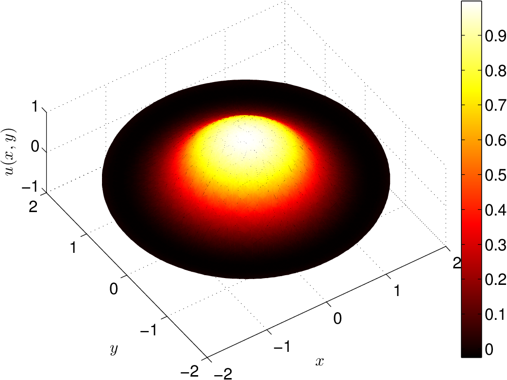
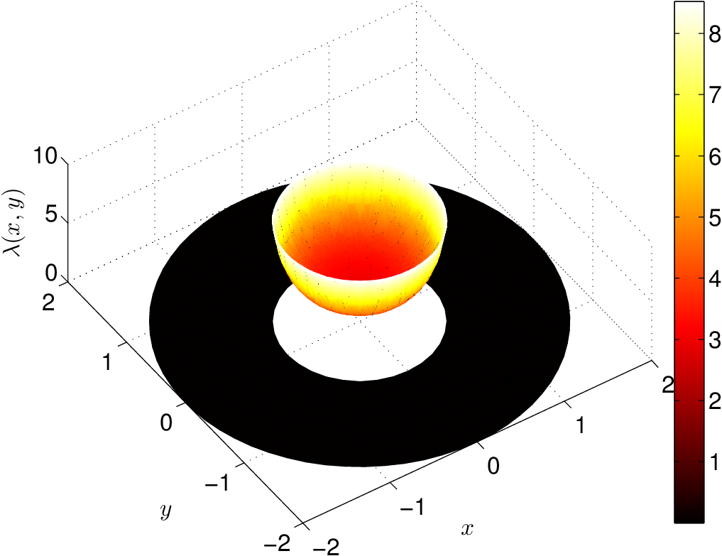
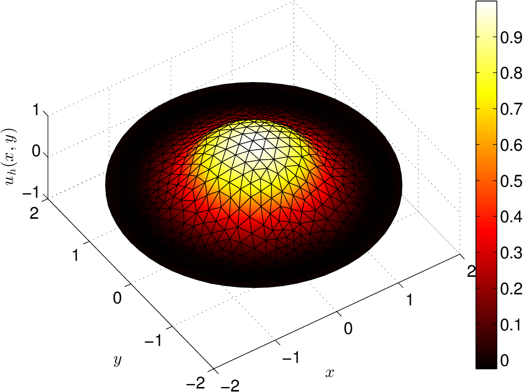
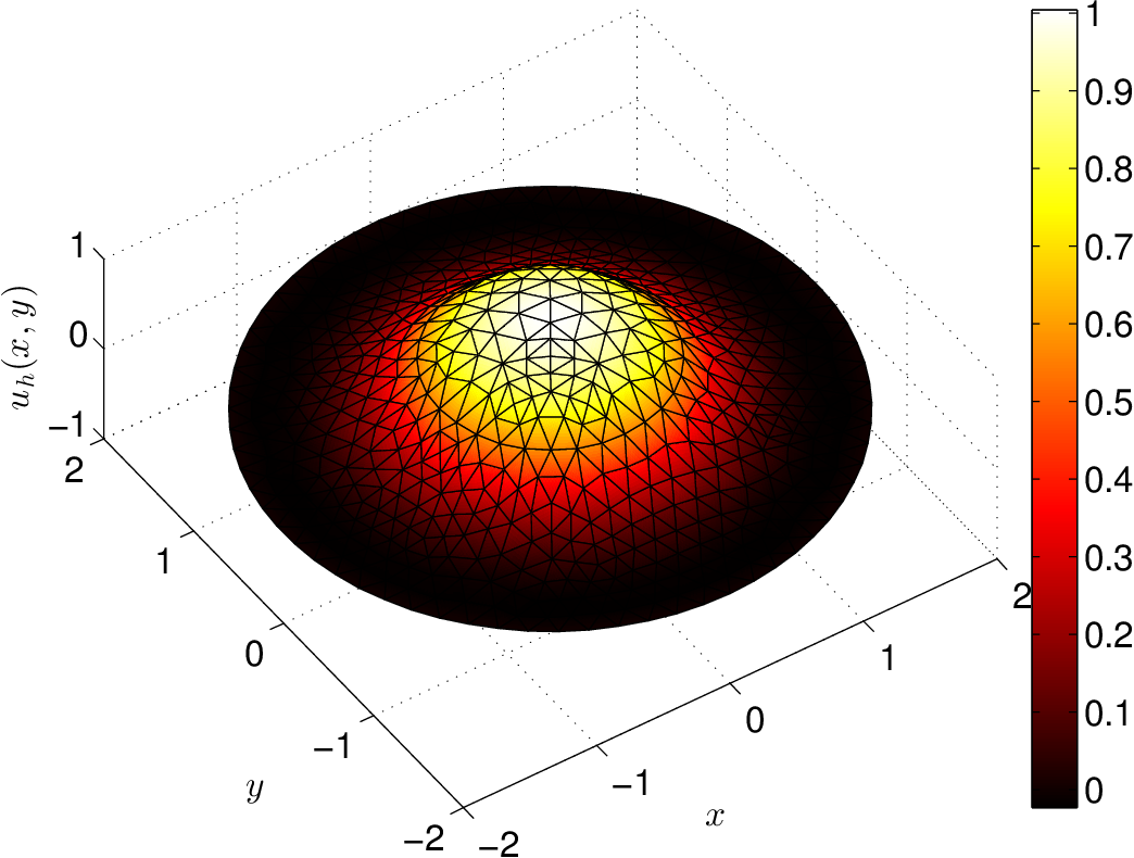
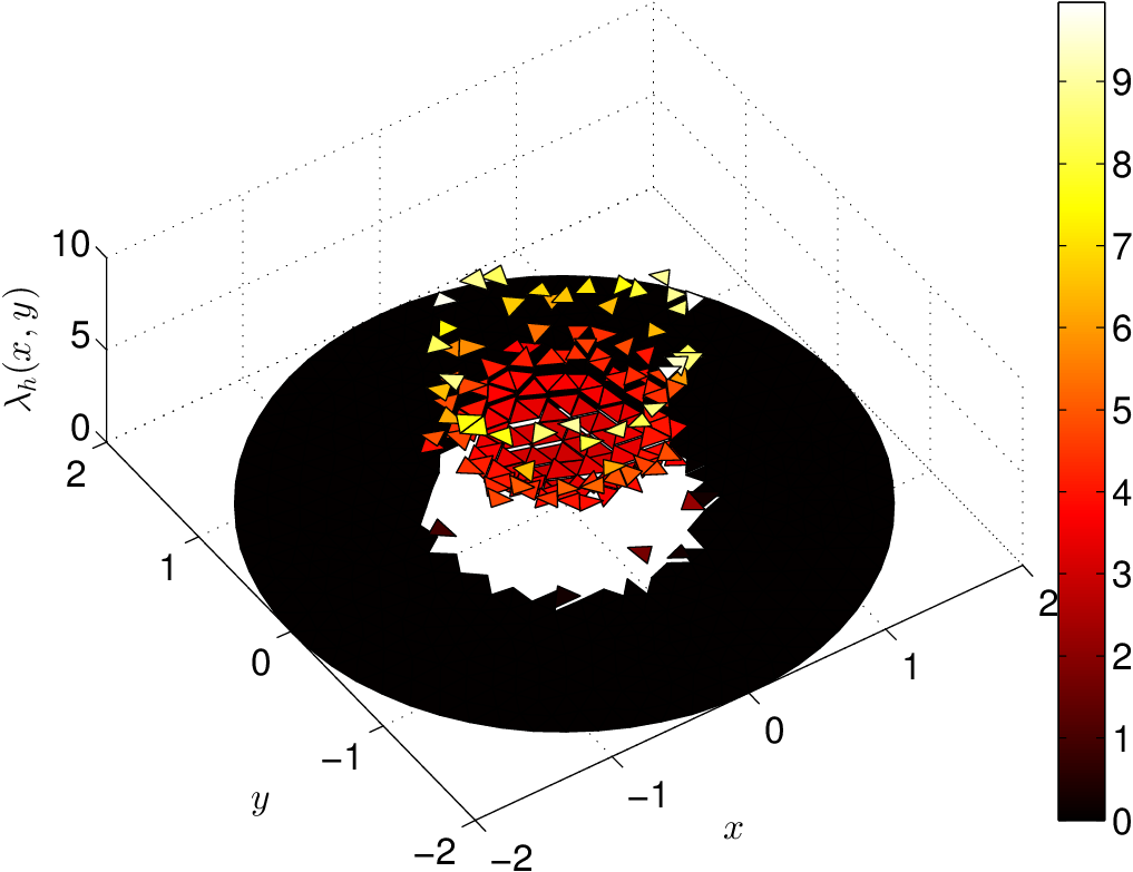
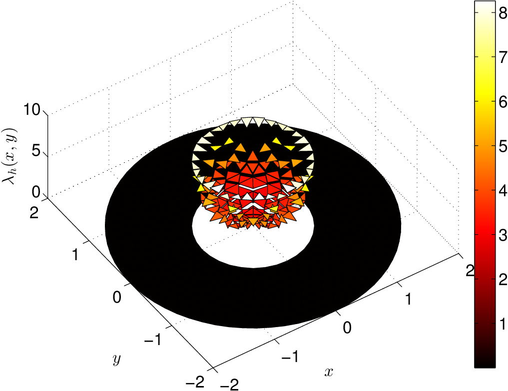
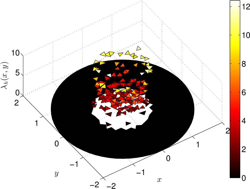
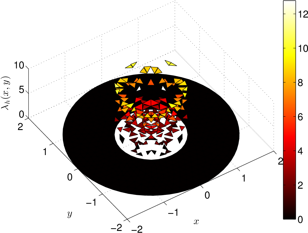
Figure 2: A comparison of analytic (upmost panel) and discrete (lower panels) solutions. The discrete solution was computed using nonconforming (left panel) and conforming (right panel) meshes and stabilized $P_{2}-P_{0}$ (third row) and $P_{1}-P_{0}$ (fourth row) methods.

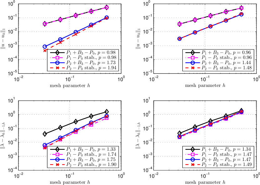
Figure 3: The convergence of the error $u-u_{h}$ in $H^{1}$-norm (upper panel) and the error $\lambda-\lambda_{h}$ in the discrete negative norm (lower panel) for the two different mesh families: conforming (left panel) and non-conforming (right panel).

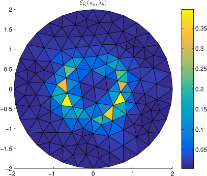
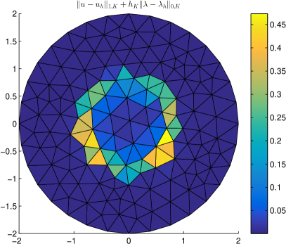
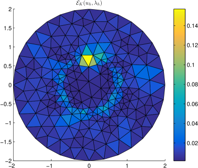
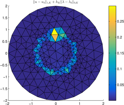
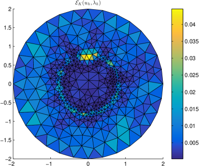
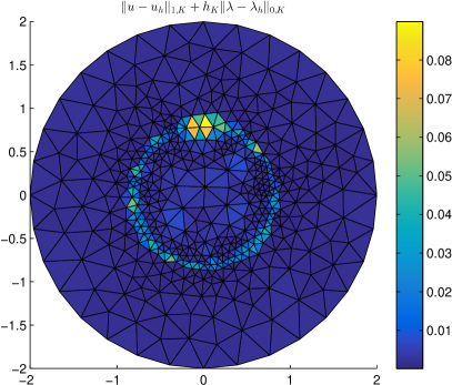
Figure 4: Three meshes arising from the adaptive refinement strategy. The local error estimators (left panels) are compared to the true local error (right panels).

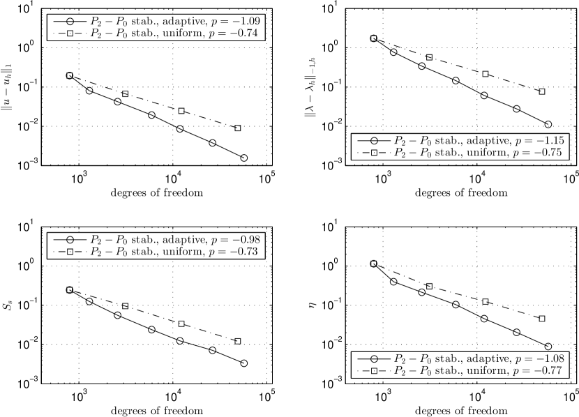
Figure 5: The convergence of the $P_{2}-P_{0}$ stabilized method with uniform and adaptive (nonconforming) refinements. The behavior of the error estimators $\eta$ and $S_{s}$ is shown separately for both cases.

Acknowledgements. Funding from Tekes – the Finnish Funding Agency for Innovation (Decision number 3305/31/2015) and the Finnish Cultural Foundation is gratefully acknowledged.

References

- [1] I. Babuška, Error-bounds for finite element method, Numer. Math., 16 (1970/1971), pp. 322–333.
- [2] , The finite element method with Lagrangian multipliers, Numer. Math., 20 (1973), pp. 179–192.
- [3] L. Banz and A. Schröder, Biorthogonal basis functions in hp-adaptive FEM for elliptic obstacle problems, Computers and Mathematics with Applications, 70 (2015), pp. 1721–1742.
- [4] L. Banz and E. P. Stephan, A posteriori error estimates of -adaptive IPDG-FEM for elliptic obstacle problems, Appl. Numer. Math., 76 (2014), pp. 76–92.
- [5] M. Benzi, G. H. Golub, and J. Liesen, Numerical solution of saddle point problems, Acta Numer., 14 (2005), pp. 1–137.
- [6] D. Braess, A posteriori error estimators for obstacle problems – another look, Numer. Math., 101 (2005), pp. 415–421.
- [7] , Finite elements, Cambridge University Press, Cambridge, third ed., 2007. Theory, fast solvers, and applications in elasticity theory, Translated from the German by Larry L. Schumaker.
- [8] H. R. Brezis and G. Stampacchia, Sur la régularité de la solution d’inéquations elliptiques, Bull. Soc. Math. France, 96 (1968), pp. 153–180.
- [9] F. Brezzi, On the existence, uniqueness and approximation of saddle-point problems arising from Lagrangian multipliers, Rev. Française Automat. Informat. Recherche Opérationnelle Sér. Rouge, 8 (1974), pp. 129–151.
- [10] F. Brezzi, W. W. Hager, and P.-A. Raviart, Error estimates for the finite element solution of variational inequalities, Numer. Math., 28 (1977), pp. 431–443.
- [11] , Error estimates for the finite element solution of variational inequalities. II. Mixed methods, Numer. Math., 31 (1978/79), pp. 1–16.
- [12] F. Brezzi and J. Pitkäranta, On the stabilization of finite element approximations of the Stokes equations, in Efficient solutions of elliptic systems (Kiel, 1984), vol. 10 of Notes Numer. Fluid Mech., Friedr. Vieweg, Braunschweig, 1984, pp. 11–19.
- [13] M. Bürg and A. Schröder, A posteriori error control of -finite elements for variational inequalities of the first and second kind, Comput. Math. Appl., 70 (2015), pp. 2783–2803.
- [14] E. Burman, P. Hansbo, M. G. Larson, and R. Stenberg, Galerkin least squares finite element method for the obstacle problem, Computer Methods in Applied Mechanics and Engineering, 313 (2016), pp. 362–374.
- [15] L. Caffarelli, The obstacle problem revisited, J. Fourier Anal. Appl., 4–5 (1998), pp. 383–402.
- [16] F. Chouly and P. Hild, A Nitsche-based method for unilateral contact problems: numerical analysis, SIAM J. Numer. Anal., 51 (2013), pp. 1295–1307.
- [17] P. Clément, Approximation of finite element functions using local regularization, RAIRO Num. Anal., 9 (1975), pp. 77–84.
- [18] L. C. Evans, An introduction to stochastic differential equations, American Mathematical Society, Providence, RI, 2013.
- [19] R. S. Falk, Error estimates for the approximation of a class of variational inequalities, Math. Comp., 28 (1974), pp. 963–971.
- [20] L. P. Franca and R. Stenberg, Error analysis of Galerkin least squares methods for the elasticity equations, SIAM J. Numer. Anal., 28 (1991), pp. 1680–1697.
- [21] , Error analysis of Galerkin least squares methods for the elasticity equations, SIAM J. Numer. Anal., 28 (1991), pp. 1680–1697.
- [22] A. Friedman, Variational principles and free-boundary problems, Pure and Applied Mathematics, John Wiley & Sons, Inc., New York, 1982. A Wiley-Interscience Publication.
- [23] R. Glowinski, Numerical Methods for Nonlinear Variational Problems, Springer-Verlag Berlin Heidenberg, 1984.
- [24] G. H. Golub and C. F. Van Loan, Matrix computations, Johns Hopkins Studies in the Mathematical Sciences, Johns Hopkins University Press, Baltimore, MD, third ed., 1996.
- [25] T. Gudi, A new error analysis for discontinuous finite element methods for linear elliptic problems, Math. Comp., 79 (2010), pp. 2169–2189.
- [26] T. Gudi and K. Porwal, A reliable residual based a posteriori error estimator for a quadratic finite element method for the elliptic obstacle problem, Comput. Methods. Appl. Math, 15 (2015), pp. 145–160.
- [27] J. Haslinger, Mixed formulation of elliptic variational inequalities and its approximation, Apl. Mat., 26 (1981), pp. 462–475.
- [28] J. Haslinger, I. Hlaváček, and J. Nečas, Numerical methods for unilateral problems in solid mechanics, in Handbook of numerical analysis, Vol. IV, Handb. Numer. Anal., IV, North-Holland, Amsterdam, 1996, pp. 313–485.
- [29] P. Hild and Y. Renard, A stabilized Lagrange multiplier method for the finite element approximation of contact problems in elastostatics, Numer. Math., 115 (2010), pp. 101–129.
- [30] M. Hintermüller, K. Ito, and K. Kunisch, The primal-dual active set strategy as semismooth newton method, SIAM J. Optim., 13 (2003), pp. 865–888.
- [31] I. Hlaváček, J. Haslinger, J. Nečas, and J. Lovíšek, Solution of variational inequalities in mechanics, vol. 66 of Applied Mathematical Sciences, Springer-Verlag, New York, 1988. Translated from the Slovak by J. Jarník.
- [32] T. J. R. Hughes and L. P. Franca, A new finite element formulation for computational fluid dynamics. VII. The Stokes problem with various well-posed boundary conditions: symmetric formulations that converge for all velocity/pressure spaces, Comput. Methods Appl. Mech. Engrg., 65 (1987), pp. 85–96.
- [33] T. J. R. Hughes, L. P. Franca, and M. Balestra, A new finite element formulation for computational fluid dynamics. V. Circumventing the Babuška-Brezzi condition: a stable Petrov-Galerkin formulation of the Stokes problem accommodating equal-order interpolations, Comput. Methods Appl. Mech. Engrg., 59 (1986), pp. 85–99.
- [34] D. Kinderlehrer and G. Stampacchia, An introduction to variational inequalities and their applications, vol. 88 of Pure and Applied Mathematics, Academic Press, Inc. [Harcourt Brace Jovanovich, Publishers], New York-London, 1980.
- [35] J.-L. Lions and G. Stampacchia, Variational inequalities, Comm. Pure Appl. Math., 20 (1967), pp. 493–519.
- [36] U. Mosco and G. Strang, One-sided approximation and variational inequalities, Bulletin of the American Mathematical Society, 80 (1974), pp. 308–312.
- [37] J. Nitsche, Über ein Variationsprinzip zur Lösung von Dirichlet-Problemen bei Verwendung von Teilräumen, die keinen Randbedingungen unterworfen sind, Abh. Math. Sem. Univ. Hamburg, 36 (1971), pp. 9–15. Collection of articles dedicated to Lothar Collatz on his sixtieth birthday.
- [38] A. Petrosyan, H. Shahgholian, and N. Uraltseva, Regularity of free boundaries in obstacle-type problems, vol. 136 of Graduate Studies in Mathematics, American Mathematical Society, Providence, RI, 2012.
- [39] R. Pierre, Simple approximations for the computation of incompressible flows, Comput. Methods Appl. Mech. Engrg., 68 (1988), pp. 205–227.
- [40] J.-F. Rodrigues, Obstacle Problems in Mathematical Physics, North-Holland Mathematics Studies, 1987.
- [41] R. Scholz, Numerical solution of the obstacle problem by the penalty method, Computing, 32 (1984), pp. 297–306.
- [42] A. Schröder, Mixed finite element methods of higher-order for model contact problems, SIAM J. Numer. Anal., 49 (2011), pp. 2323–2339.
- [43] R. Stenberg, A technique for analysing finite element methods for viscous incompressible flow, Internat. J. Numer. Methods Fluids, 11 (1990), pp. 935–948. The Seventh International Conference on Finite Elements in Flow Problems (Huntsville, AL, 1989).
- [44] , On some techniques for approximating boundary conditions in the finite element method, J. Comput. Appl. Math., 63 (1995), pp. 139–148. International Symposium on Mathematical Modelling and Computational Methods Modelling 94 (Prague, 1994).
- [45] R. Stenberg and J. Videman, On the error analysis of stabilized finite element methods for the Stokes problem, SIAM J. Numer. Anal., 53 (2015), pp. 2626–2633.
- [46] M. Ulbrich, Semismooth Newton Methods for Variational Inequalities and Constrained Optimization Problems in Function Spaces, MOS-SIAM Series on Optimization, 2011.
- [47] A. Veeser, Efficient and reliable a posteriori error estimators for elliptic obstacle problems, SIAM J. Numer. Math., 39 (2001), pp. 146–167.
- [48] A. Weiss and B. Wohlmuth, A posteriori error estimator for obstacle problems, SIAM J. Sci. Comput., 32 (2010), pp. 2627–2658.
- [49] B. Wohlmuth, Variationally consistent discretization schemes and numerical algorithms for contact problems, Acta Numerica, 20 (2011), pp. 569–734.