Non-equilibrium ionization by a periodic electron beam

Abstract

Context. Coronal heating is currently thought to proceed via the mechanism of nanoflares, small-scale and possibly recurring heating events that release magnetic energy.

Aims. We investigate the effects of a periodic high-energy electron beam on the synthetic spectra of coronal Fe ions.

Methods. Initially, the coronal plasma is assumed to be Maxwellian with a temperature of 1 MK. The high-energy beam, described by a $\kappa$-distribution, is then switched on every period $P$ for the duration of $P/2$. The periods are on the order of several tens of seconds, similar to exposure times or cadences of space-borne spectrometers. Ionization, recombination, and excitation rates for the respective distributions are used to calculate the resulting non-equilibrium ionization state of Fe and the instantaneous and period-averaged synthetic spectra.

Results. Under the presence of the periodic electron beam, the plasma is out of ionization equilibrium at all times. The resulting spectra averaged over one period are almost always multithermal if interpreted in terms of ionization equilibrium for either a Maxwellian or a $\kappa$-distribution. Exceptions occur, however; the EM-loci curves appear to have a nearly isothermal crossing-point for some values of $\kappa_{\mathrm{s}}$. The instantaneous spectra show fast changes in intensities of some lines, especially those formed outside of the peak of the respective EM$(T)$ distributions if the ionization equilibrium is assumed.

1 Introduction

The solar corona, the upper atmosphere of the Sun, has temperatures of up to several million Kelvin. Its radiation is characterized by a large number of emission lines originating from multiply ionized metal ions, such as Fe, Ca, and Si (e.g., Landi et al., 2002; Curdt et al., 2004; Landi & Young, 2009). This emission typically comes from coronal loops and unresolved background located within active regions (see, e.g., Del Zanna & Mason, 2003; Cirtain, 2005; Young et al., 2009, 2012; Tripathi et al., 2009; Schmelz et al., 2009, 2011; Warren et al., 2012; Ugarte-Urra & Warren, 2012; Teriaca et al., 2012; Del Zanna, 2013b; Subramanian et al., 2014; Gupta et al., 2015, for recent observations).

It is currently thought that the active region corona is heated by nanoflares, i.e., impulsive and possibly recurring processes of unknown origin releasing small quantities of magnetic energy (e.g., Parker, 1988; Cargill, 1994; Cargill & Klimchuk, 2004; Cargill, 2014; Klimchuk, 2006; Klimchuk et al., 2010; Tripathi et al., 2010; Warren et al., 2011; Viall & Klimchuk, 2011a, b, 2015; Bradshaw et al., 2012; Reep et al., 2013; Winebarger et al., 2013; Testa et al., 2013; Klimchuk, 2015). It has been recognized that such impulsive energy releases could occur on timescales shorter than the ionization equilibration timescales (e.g., Bradshaw & Mason, 2003b; Bradshaw & Cargill, 2006; Reale & Orlando, 2008; Smith & Hughes, 2010; Bradshaw & Klimchuk, 2011), leading to significant departures of the ion composition of the plasma from its equilibrium value for the given local electron temperature. This non-equilibrium ionization must then be taken into account when modeling the solar corona and the arising spectra (see, e.g., Bradshaw & Mason, 2003a; Bradshaw, 2009; Olluri et al., 2013b, a, 2015).

The presence of the non-equilibrium ionization, however, may not be the only difficulty connected to the impulsive energy release in nanoflares. Accelerated particles may be present as well, especially if the nanoflares happen via magnetic reconnection (e.g., Fletcher et al., 2011; Cargill et al., 2012; Gontikakis et al., 2013; Gordovskyy et al., 2013, 2014; Burge et al., 2014), wave-particle interactions (Vocks et al., 2008; Che & Goldstein, 2014), or turbulence with a diffusion coefficient inversely proportional to velocity (Hasegawa et al., 1985; Laming & Lepri, 2007; Bian et al., 2014). The presence of energetic particles have been indirectly detected using analyses of emission lines originating in active regions (Dzifčáková et al., 2011; Testa et al., 2014; Dudík et al., 2015).

Nevertheless, the current analyses of coronal spectra are subject to various difficulties and uncertainties involved and therefore the departures from equilibrium are still largely ignored. This paper presents an exploratory study of the combined effects of energetic particles and the non-equilibrium ionization on the coronal spectra. A simple model of a periodic electron beam is assumed in Sect. 2. The resulting behavior of the non-equilibrium plasma is described in Sect. 3, while the consequences for interpretation of observed spectra are given in Sect. 4. A summary is presented in Sect. 5.

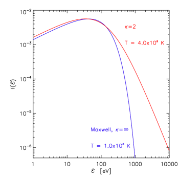
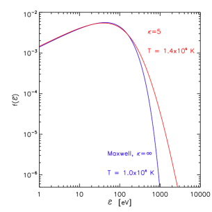
Figure 1: Electron energy distributions considered in the model. The Maxwellian distribution with $T$ = 1 MK is shown in blue, while the $\kappa$-distributions with $\kappa$ = 2 and 5 are shown in the left and right panels, respectively. The corresponding temperatures of the $\kappa$-distributions are indicated.

2 Method

2.1 Periodic electron beam

We consider a simple model where an electron beam passing through the plasma is periodically “switched on” and then “switched off” with a fixed period $P$. Initially, and when the beam is switched off, the plasma is assumed to have a Maxwellian distribution with a temperature $T$ = 1 MK. This temperature is chosen arbitrarily to represent, for example, a typical temperature of a warm coronal loop as derived from observations (e.g., Del Zanna & Mason, 2003; Del Zanna, 2013b; Warren & Winebarger, 2003; Winebarger et al., 2003; Aschwanden & Nightingale, 2005; Aschwanden et al., 2008; Schmelz et al., 2009, 2011; Landi & Young, 2010; Brooks et al., 2011, 2012).

At time $t$ = 0, the electron beam is switched on for the duration of a half-period $P/2$. The electron beam is represented by power-law high-energy tail described by a $\kappa$-distribution (e.g., Vasyliunas, 1968; Owocki & Scudder, 1983; Dzifčáková et al., 2015)

$$f_{\kappa}(E)dE=A_{\kappa}C_{\kappa}\frac{2}{\sqrt{\pi}\left(k_{\mathrm{B}}T_{\kappa}\right)^{3/2}}\frac{E^{1/2}dE}{\left(1+\frac{E}{(\kappa-3/2}k_{\mathrm{B}}T_{\kappa}\right)^{\kappa+1}}\,,$$ (1)

where $A_{\kappa}$ is a normalization constant, $k_{\mathrm{B}}$ is the Boltzmann constant, $C_{\kappa}$ is a multiplication constant determined by matching the peak of the $\kappa$-distribution to the peak of the Maxwellian (Fig. 1), and $T_{\kappa}$ is the temperature of the $\kappa$-distribution that is in principle different from the chosen $T$ = 1 MK for the Maxwellian distribution. The slope of the power-law tail of the $\kappa$-distribution is given by $\kappa+1/2$.

The choice of a $\kappa$-distribution to describe the power-law high-energy tail is made because the $\kappa$-distribution is a distribution with a Maxwellian-like bulk (Oka et al., 2013) and a strong high-energy tail while still being continuous and described by only one extra free parameter, $\kappa$. The values of $C_{\kappa}$ and $T_{\kappa}$ are then dependent on the value of $\kappa$ chosen, with

$$T_{\kappa} = \frac{\kappa}{\kappa-3/2}T,$$ (2)

$$C_{\kappa} = \mathrm{exp}(-1)\frac{\Gamma(\kappa-1/2)}{\Gamma(\kappa+1)}\kappa^{3/2}\left(1+\frac{1}{\kappa}\right)^{\kappa+1},$$ (3)

(cf., Oka et al., 2013). For $\kappa$ = 2, the temperature $T_{\kappa}$ is 4 MK, while for $\kappa$ = 5, it is approximately 1.4 MK. It is not surprising that these $T_{\kappa}$ values are higher than the Maxwellian $T$, since the switch-on of the electron beam effectively adds energetic particles to the emitting plasma considered. The $\kappa$-distributions with $\kappa$ = 5 and 2 adds 19% and 56% particles, respectively (see Eq. 3). Most of these particles are added at energies of several keV or below (see Fig. 1), i.e., at energies undetectable by RHESSI (cf., Hannah et al., 2010).

We note that we do not consider the evolution of the distribution function because of the collisions of the high-energy electrons with the ambient Maxwellian. This is of course only a crude approximation that is analogous to assuming that the $\kappa$-distribution is being generated for the duration of $P/2$ somewhere else along the emitting loop, passes through the plasma whose radiation is being investigated, exits the region of interest after $P/2$, and is thermalized in the chromosphere. Our aim is only to explore the possible effects of periodic electron beams on the coronal spectra without constructing a too specific coronal loop model including geometry, hydrodynamic evolution, and details of particle acceleration and interaction.

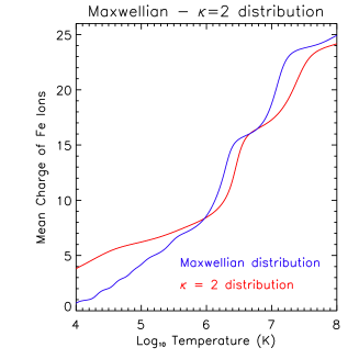
Figure 2: Mean charge of iron in ionization equilibrium as a function of electron temperature for the Maxwellian (blue) and a $\kappa$-distribution with $\kappa$ = 2 (red).

2.2 Non-equilibrium ionization and the effective temperature

At $t$ = 0, the plasma is assumed to be in collisional ionization equilibrium corresponding to the Maxwellian with $T$ = 1 MK. The corresponding relative ion abundances and the ionization and recombination cross-sections are given by the atomic data present in the CHIANTI database, version 7.1 (Dere et al., 1997; Dere, 2007; Landi et al., 2013). At $t$ = 0, the beam is switched on, resulting in a change of the electron distribution including $T$ $\to$ $T_{\kappa}$, with the ionization and recombination rates changing correspondingly. If the period $P$ is less than the ionization equilibration timescale (e.g., Golub et al., 1989; Reale & Orlando, 2008; Smith & Hughes, 2010), the plasma is no longer in ionization equilibrium. These equilibration timescales are typically tens or hundreds of seconds, depending on the temperature, density, and element considered (see Fig. 1 in Smith & Hughes, 2010).

We consider the following equation for ionization non-equilibrium (e.g., Bradshaw & Mason, 2003a, b; Smith & Hughes, 2010)

$$\frac{dY_{i}}{dt}=n_{\mathrm{e}}\left(I_{i-1}Y_{i-1}+R_{i+1}Y_{i+1}-I_{i}Y_{i}-R_{i}Y_{i}\right)\,,$$ (4)

where $Y_{i}$ is the relative ion abundance of the $i$-times ionized ion of the element $Y$, with $\sum_{i}Y_{i}=1$, $n_{\mathrm{e}}$ is electron number density, and $I_{i}$ and $R_{i}$ are the total ionization and recombination coefficients from the ion stage $+i$. The advective term is not considered as we do not consider any specific hydrodynamic model of a coronal loop.

The ionization and recombination processes considered include the direct impact ionization, autoionization, and radiative and dielectronic recombination. For the Maxwellian distribution, these rates are obtained from the CHIANTI database, while for the $\kappa$-distributions the rates were obtained by Dzifčáková & Dudík (2013).

We note that the electron density $n_{\mathrm{e}}$ is not constant throughout the period $P$. In the first half-period, where the distribution is a $\kappa$-distribution, the $n_{\mathrm{e}}$ is $C_{\kappa}$-times higher than during the second, Maxwellian half-period because the change of the distribution to a $\kappa$-one effectively adds particles (Fig. 1). The first-order differential equation (4) is then solved using the Runge-Kutta method with a sufficiently small time step ensuring the stability of the solution and the condition that $\sum_{i}Y_{i}$ = 1 is fulfilled at every time step.

To describe the non-equilibrium ionization state, we used the effective ionization temperature. In ionization equilibrium, the mean charge state of an element is a monotonically increasing function of electron temperature. The shape of the curve depends on $\kappa$; an example for iron is shown in Fig. 2. For $\kappa$ = 2 and log($T$/K) $\lesssim$ 6.2, it is shallower than for the Maxwellian distribution. This is a consequence of the shift of the equilibrium relative ion abundances of Fe towards lower $T$ for low values of $\kappa$ (Dzifčáková & Dudík, 2013). At higher temperatures, the curve is similar to the one for the Maxwellian distribution, but is shifted towards higher $T$ for low values of $\kappa$, again a consequence of the behavior of the ionization equilibrium with $\kappa$.

The monotonic nature of these curves permits us to define the effective temperatures $T_{\mathrm{eff}}^{\kappa=\mathrm{const.}}$ for a respective $\kappa$-distribution. We define it as the temperature corresponding to a particular mean charge of an element if interpreted in terms of ionization equilibrium for a given value of $\kappa$. We note that in ionization equilibrium, the effective ionization temperature is by definition equal to the electron temperature if a correct value of $\kappa$ is used.

In the remainder of this work, we study the non-equilibrium ionization of iron under a periodic electron beam (Sect. 3). The $T_{\mathrm{eff}}$ is calculated from the mean Fe charge in the non-equilibrium ionization state under the assumption that the plasma is either Maxwellian or non-Maxwellian with a constant value of $\kappa$, as done when interpreting the coronal observations (see, e.g., Dudík et al., 2015).

2.3 Synthesis of coronal spectra

Once the relative ion abundances $Y_{i}$ are obtained, we calculate the synthetic Fe VIII–Fe XVII line spectra at wavelengths of 170–290 Å, similar to the wavelength range observed by the Extreme-ultraviolet Imaging Spectrometer (EIS, Culhane et al., 2007) onboard the Hinode satellite (Kosugi et al., 2007). The emissivities $\varepsilon_{i,jk}$ of the Fe lines arising due to the transition $j$ $\to$ $k$ in the ion $Y_{i}$ in the optically thin coronal conditions are given by (e.g., Mason & Mosignori-Fossi, 1994; Phillips et al., 2008)

$$\varepsilon_{i,jk}=\frac{hc}{\lambda_{jk}}\frac{A_{jk}}{n_{\mathrm{e}}}\frac{n_{j}}{n_{i}}Y_{i}A_{\mathrm{Fe}}n_{\mathrm{e}}n_{\mathrm{H}}=A_{\mathrm{Fe}}G_{i,jk}(T,n_{\mathrm{e}},\kappa)n_{\mathrm{e}}n_{\mathrm{H}}\,,$$ (5)

where $\lambda_{jk}$ is the wavelength of the transition, $h$ is the Planck constant, $c$ is the speed of light, $n_{\mathrm{H}}$ is the hydrogen number density, $n_{j}$ is the number density of the $i$-times ionized Fe ion with the electron on the excited upper level $j$, $n_{i}$ = $Y_{i}n_{\mathrm{Fe}}$ and $A_{\mathrm{Fe}}$ = $n_{\mathrm{Fe}}/n_{\mathrm{H}}$ is the iron abundance relative to hydrogen, and $G_{i,jk}(T,n_{\mathrm{e}},\kappa)$ is the line contribution function. The Einstein’s coefficients $A_{jk}$ for the spontaneous radiative transition are taken from the CHIANTI database, version 7.1 (Dere et al., 1997; Landi et al., 2013), as are the collisional excitation and deexcitation rates for the Maxwellian distribution. For the $\kappa$-distributions, these collisonal excitation and deexcitation rates are obtained using the approximative method implemented in the KAPPA database (Dzifčáková et al., 2015). It was shown therein that the relative accuracy of the rates obtained using this approximative method are typically higher than 5% when compared to the rates obtained by direct calculations from the respective cross-sections (Dudík et al., 2014b). We note however that some of the excitation rates have been recently updated in the version 8 of the CHIANTI database (Del Zanna et al., 2015). The influence of these new atomic data on the resulting spectra is discussed in Appendix A. Finally, we adopted the “coronal” value of $A_{\mathrm{Fe}}$ based on the abundance measurements of Feldman et al. (1992).

The corresponding line intensities $I_{i,jk}$ are then obtained by using the formula

$$I_{i,jk}=A_{\mathrm{Fe}}\int_{l}G_{i,jk}(T,n_{\mathrm{e}},\kappa)n_{\mathrm{e}}n_{\mathrm{H}}dl\,,$$ (6)

where $l$ is the observer’s line of sight through the optically thin corona. We note that this equation is commonly recast as

$$I_{i,jk}=A_{\mathrm{Fe}}\int_{T}G_{i,jk}(T,n_{\mathrm{e}},\kappa)\mathrm{DEM}_{\kappa}(T)dT\,$$ (7)

for the purpose of intepretation of observations. Here, the quantity DEM${}_{\kappa}(T)=n_{\mathrm{e}}n_{\mathrm{H}}dl/dT$ is the differential emission measure (see, e.g., chapter 4.6 in Phillips et al., 2008), generalized for the $\kappa$-distributions by Mackovjak et al. (2014). The corresponding emission measure EM${}_{\kappa}(T)$ is then simply given as EM${}_{\kappa}(T)$ = DEM${}_{\kappa}(T)dT$.

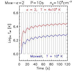
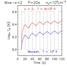
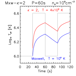
Figure 3: Evolution of the effective ionization temperature (left) and the corresponding EUV spectra during the first (center) and fifth period (right). Individual rows stand for different periods. The assumed electron density is log$(n_{\mathrm{e}}$ [cm^-3]) = 9. Instantaneous spectra at each time step in the calculation are shown in Movies 1–3.

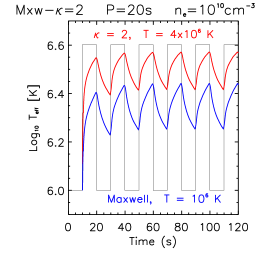
Figure 4: Same as in Fig. 3, but for log$(n_{\mathrm{e}}$ [cm^-3]) = 10. The corresponding instantaneous spectra are shown in Movie 4.

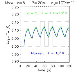
Figure 5: Same as in Fig. 3, but for $\kappa$ = 5. The corresponding instantaneous spectra are shown in Movie 5.

3 Results

3.1 Results for strong beam

To explore the consequences of a periodic high-energy electron beam, we studied several cases described by their respective free parameters. First, we chose the electron density to be $n_{\mathrm{e}}$ = 10⁹ cm^-3, a value typical of the solar corona (e.g., Landi & Landini, 2004; Tripathi et al., 2009; Shestov et al., 2009; O’Dwyer et al., 2011; Dudík et al., 2015; Gupta et al., 2015). This value pertains to the half-period during which the distribution is a $\kappa$-distribution. Next, we selected $\kappa$ = 2, which is the most extreme non-Maxwellian value for which the spectra can be synthesized using the KAPPA package (Dzifčáková et al., 2015). Finally, we chose periods on the order of several tens of seconds to be comparable with the typical exposure times and/or cadence of the EUV coronal spectrometers such as Hinode/EIS (except perhaps for observations of brightest lines, see Culhane et al., 2007) or imagers such as SDO/AIA (Lemen et al., 2012; Boerner et al., 2012). We note that such periods are also of the same order of magnitude as the durations of individual nanoflare heating events (e.g., Bradshaw & Mason, 2003b; Bradshaw & Cargill, 2006; Taroyan et al., 2006, 2011; Reale & Orlando, 2008; Bradshaw, 2009; Bradshaw & Klimchuk, 2011; Bradshaw et al., 2012; Reep et al., 2013; Klimchuk & Bradshaw, 2014; Price et al., 2015).

Figure 3 shows the results for $P$ = 10, 20, and 60 s. Although these values are arbitrary, they are sufficient to capture the typical effects of the periodic electron beam on the spectra. In this figure, the left panel shows the stepwise evolution of the distribution function together with the effective ionization temperatures calculated under the assumption of a $\kappa$ = 2 distribution and a Maxwellian distribution. The middle and right panels show the corresponding spectra averaged over the first and fifth period, respectively. The respective instantaneous spectra at each time step are shown as animations in Movies 1-3.

For the shortest period of 10 s, we find that the $P$ is short enough for the plasma to be out of ionization equilibrium and that it undergoes ionization pumping. This means that during the first half-period $P/2$, when the beam is switched on, the effective ionization temperatures calculated for $\kappa$ = 2 and the Maxwellian distribution both spike from the initial value of $T$ = 1 MK and reach log($T_{\mathrm{eff}}^{\kappa=2}$ [K]) $\approx$ 6.35 and log($T_{\mathrm{eff}}^{\mathrm{Mxw}}$ [K]) $\approx$ 6.17 (Fig. 3, top left, and Movie 1). This is followed by a small drop in the second-half period during which the beam is switched off and the distribution is Maxwellian. In the subsequent periods, the effective ionization temperature continues to rise at a slowing rate until it reaches the maximum values of log($T_{\mathrm{eff}}^{\kappa=2}$ [K]) $\approx$ 6.45 and log($T_{\mathrm{eff}}^{\mathrm{Mxw}}$ [K]) $\approx$ 6.3. There are, however, small saw-like variations in $T_{\mathrm{eff}}$ due to the periodic switching on and off of the beam, so that the plasma is never in ionization equilibrium.

The corresponding spectra averaged over the first and fifth periods are shown in the top row of Fig. 3. During the first period, the average spectrum (black) is dominated by the strong Fe IX–Fe XII lines at 171–195 Å; the Fe XI 180.40 Å line is the strongest one. The higher temperature lines are much weaker, having less than 20% in terms of intensity than the strongest Fe XI line. The Fe XV 284.16 Å line is very weak, having less than about 5% relative intensity. These intensities are not surprising given the values of $T_{\mathrm{eff}}$ during the first period, since this quantity is based on the mean ion charge (see Sect. 2.2).

In contrast, the average spectrum for the fifth period is significantly different. We note that the fifth period is chosen as a representative one and has an average log($T_{\mathrm{eff}}$ [K]), which is not significantly different from the near stationary behavior of the ionization composition, which is lower by less than 0.05 dex. The period-averaged spectrum is now dominated by the Fe XI–Fe XV lines (Fig. 3 top right). The Fe XI 180.40 Å line is still the dominant one, but the intensities of lines belonging to the higher ionization stages have increased significantly, while the Fe IX and Fe X lines have decreased. In particular, the relative intensity of the Fe XV 284.16 Å line is now 0.7. The instantaneous spectra (Movie 1) show fast, subsecond changes especially in the Fe IX 171.07 Å and Fe XV 284.16 Å lines during the first period. These changes are slower during the subsequent periods, when the intensity of Fe XV 284.16 Å line increases.

For $P$ = 20 s, the situation is similar to that of $P$ = 10 s discussed previously, except that the effect of ionization pumping is now weaker. The log$(T_{\mathrm{eff}}^{\kappa=2})$ [K]) reaches a maximum of $\approx$6.4 during the first period and 6.45 during the fifth period, while the maxima of the log$(T_{\mathrm{eff}}^{\mathrm{Mxw}})$ [K]) $\approx$ 6.23 and 6.3 for the first and fifth period, respectively. The intensities of the Fe XIII–Fe XV lines increase with respect to the $P$ = 10 s case, with the Fe XV 284.16 Å line having almost 1.0 relative intensity during the fifth period. The instantaneous spectra show a fast decrease in the Fe IX 171.07 Å line during the first 5 seconds, followed by the appearance of the Fe XV line. The intensity of this line increases on average from the first half-period, and decreases when the distribution is Maxwellian. In the second and subsequent periods the line remains visible, as can be expected from the behavior of the $T_{\mathrm{eff}}$.

The $P$ = 60 s period case exhibits a fast increase in $T_{\mathrm{eff}}$ during the first period to log($T_{\mathrm{eff}}^{\kappa=2}$ [K]) of about 6.45 and log($T_{\mathrm{eff}}^{\mathrm{Mxw}}$ [K]) $\approx$ 6.3, followed by a decrease of about 0.1 dex during the second half-period. In the next periods, the effective temperatures increase to similar maximum values and an oscillatory state is reached within the second period. The averaged spectra are now dominated by the Fe XV 284.16 Å line, with the intensities of lower ionization stages being weaker during the fifth period than during the first period (see the bottom row of Fig. 3). The Fe IX 171.07 Å, Fe XI 180.40 Å, and Fe XII 195.12 Å lines nevertheless remain relatively strong with the relative intensities of about 0.6.

In the instantaneous spectra, however, the Fe IX–Fe XII lines are dominant over the first 12 seconds. During this time, their intensities decrease, while the intensity of Fe XV increases and is dominant approximately in the interval of 12–50 s. After the first half-period (30 s), the Fe XV line intensity decreases and the last 10 seconds of the period are again dominated by lower ionization stages, in particular Fe IX. These changes reflect again the evolution of $T_{\mathrm{eff}}$.

In all the cases presented here, the $T_{\mathrm{eff}}$ is different from the respective $T_{\kappa}$ or $T$, indicating that the plasma is always out of ionization equilibrium.

3.2 Higher electron density

To study the influence of electron density on the evolution, we present the case of $P$ = 20 s calculated assuming an order of magnitude higher density of log($n_{\mathrm{e}}$ [cm^-3]) = 10. The results are shown in Fig. 4.

In this case, the maximum $T_{\mathrm{eff}}$ reaches higher values during the first period compared to the case with lower density, with log$(T_{\mathrm{eff}}^{\kappa=2}$ [K]) = 6.55 and log$(T_{\mathrm{eff}}^{\mathrm{Mxw}}$ [K]) = 6.40. In particular, the value of $T_{\mathrm{eff}}^{\kappa=2}$ is significantly closer to the respective equilibrium value for the first half-period. The enhanced electron density, however, also leads to enhanced recombination. The recombination, dominant in the second half-period, causes a larger drop in $T_{\mathrm{eff}}$, of about 0.15 dex, than in the case with lower density. In the subsequent periods, the maximum values of $T_{\mathrm{eff}}^{\kappa=2}$ increase slightly owing to the weak ionization pumping, but never reach the respective equilibrium value (left panel in Fig. 4).

The average spectra are dominated by Fe XV, in agreement with the values of $T_{\mathrm{eff}}$, but show significant Fe IX 171.07 Å intensities as well. The intensity of this Fe IX spikes and becomes temporarily dominant in the second half-period for the last 6 seconds owing to the enhanced recombination.

Increasing the density by another order of magnitude to 10¹¹ cm^-3 would cause the $T_{\mathrm{eff}}^{\kappa=2}$ to temporarily reach its equilibrium value of 4 MK for nearly the entire second quarter of a period, while the $T_{\mathrm{eff}}^{\mathrm{Mxw}}$ would approach its equilibrium value of 1 MK towards the end of the first period. This means that a sufficient increase in electron density would lead to the plasma being in ionization equilibrium for a non-negligible portion of the half-period, characterized by its respective distribution.

3.3 A weaker beam

To study the effects of weaker beam, we selected $\kappa$ = 5, which is an intermediate value of $\kappa$ in terms of the influence of stationary $\kappa$-distributions on spectra (Dzifčáková & Dudík, 2013; Dudík et al., 2014a, b). The other parameters are set to be log($n_{\mathrm{e}}$ [cm^-3]) = 9 and $P$ = 20 s.

Owing to the lower number of high-energy particles in a $\kappa$ = 5 distribution, the $T_{\mathrm{eff}}$ does not attain values larger than 6.12 in the log. The values of $T_{\mathrm{eff}}^{\kappa=5}$ and $T_{\mathrm{eff}}^{\mathrm{Mxw}}$ are only marginally different, which is likely due to the behavior of the ionization equilibrium (Dzifčáková & Dudík, 2013) and thus the mean ion charge used to define the $T_{\mathrm{eff}}$. The averaged spectra are dominated by the Fe IX line; the Fe XIII–Fe XV lines are strongly suppressed corresponding to the relatively low values of $T_{\mathrm{eff}}$. The spectra of the first and fifth period are similar, which is expected given the absence of a strong ionization pumping. In the instantaneous spectra (Movie 5), the Fe IX 171.07 Å line intensity oscillates by more than a factor of two, while the intensity of the Fe X 174.53 Å line exhibits much weaker changes on the order of 20%.

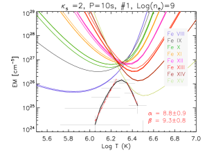
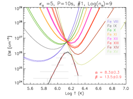
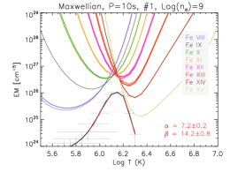
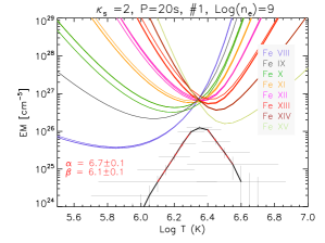
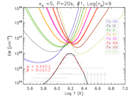
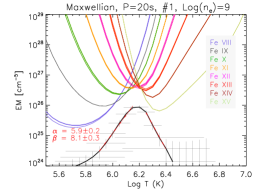
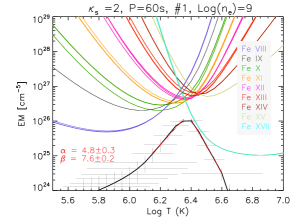
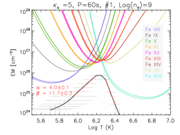
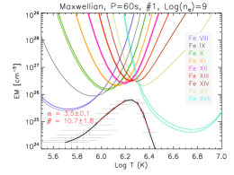
Figure 6: Emission measure distributions EM($T$) derived under the assumption of a constant $\kappa_{\mathrm{s}}$ using the intensities averaged over the first period for $P$ = 10 s (top), 20 s (middle), and 60 s (bottom). The spectra correspond to log$(n_{\mathrm{e}}$ [cm^-3]) = 9. Low-$T$ and high-$T$ power-law slopes of the EM($T$) functions are denoted $\alpha$ and $\beta$, respectively.

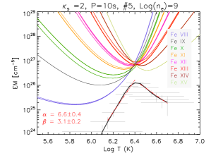
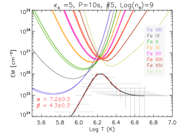
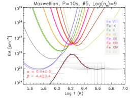
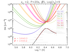
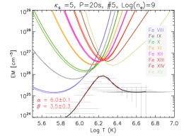
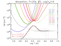
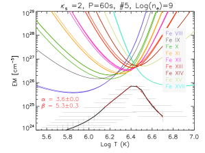
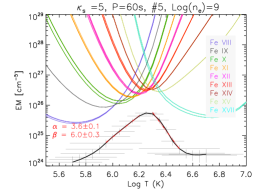
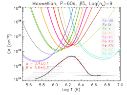
Figure 7: Same as in Fig. 6, but for the fifth period.

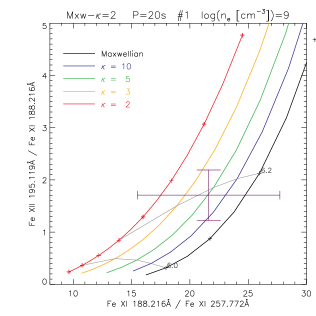
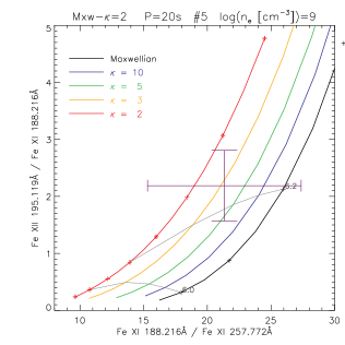
Figure 8: Attempted diagnostics of a stationary $\kappa$-distribution using the period-averaged spectra for the first period (left) and the fifth period (right). Individual colors stand for different values of the stationary $\kappa$-distribution, while the violet cross represents the line intensity ratios with their assumed uncertainties.

4 Consequences for interpretation of observations

In Sect. 3 it was found that all the studied cases are out of ionization equilibrium at all times, and that the respective period-averaged spectra show the presence of lines from multiple ionization stages. We now focus on the interpretation of such spectra, both in terms of plasma multithermality, i.e., using DEM techniques, as well as in terms of diagnosing possible departures from the Maxwellian distribution.

4.1 Multithermality

We first used the period-averaged synthetic intensities to calculate the respective DEMs as a function of $\kappa_{\mathrm{s}}$. Here, we use $\kappa_{\mathrm{s}}$ to denote to a stationary $\kappa$-distribution, i.e., a distribution of electron energies with a constant value of $\kappa_{\mathrm{s}}$, assumed by the prospective observer in analysis of the spectra. This analysis was used by Mackovjak et al. (2014) on the spectra of active region cores and quiet Sun presented by Warren et al. (2012) and Landi & Young (2010), respectively. Mackovjak et al. (2014) found that the slopes of the EM($T$) for the multithermal active region cores did not change with $\kappa_{\mathrm{s}}$, while the quiet Sun spectra were multithermal with a decreasing degree of multithermality with decreasing $\kappa_{\mathrm{s}}$.

In Figs. 6 and 7, we present the EM($T$) distributions calculated using the synthetic intensities from the synthetic spectra presented in Fig. 3, i.e., a periodic beam with $\kappa$ = 2 and log($n_{\mathrm{e}}$ [cm^-3]) = 9. The EM($T$) distributions presented in Fig. 6 correspond to the intensities averaged over the first period, reflecting the case of a single pulse, while those in Fig. 7 correspond to the intensities averaged over the fifth period, representing a near-stationary oscillatory state. The EM($T$) distributions shown in Figs. 6 and 7 were obtained from the respective DEM($T$) calculated using the regularized inversion method of Hannah & Kontar (2012) under the assumption of a constant $\kappa_{\mathrm{s}}$ value. We note that the $\kappa_{\mathrm{s}}$ influences the line contribution functions, which are calculated using the method described in Dzifčáková et al. (2015) under the assumption of the ionization equlibrium. The values of $\kappa_{\mathrm{s}}$ used for the construction of these EM$(T)$ distributions are $\kappa_{\mathrm{s}}$ = 2 (left column), 5 (middle), and $\infty$, i.e., a Maxwellian distribution (right column).

We find that for nearly all the cases presented in Figs. 6 and 7, the plasma is multithermal. The low-temperature and high-temperature slopes, $\alpha$ and $\beta$, respectively, are indicated in each panel of Figs. 6 and 7. These slopes and their respective errors are obtained by linear least-square fitting of the log(EM) as a function of log($T$ [K]). For $P$ = 10, the EM$(T)$ distributions are near-isothermal (cf., Warren et al., 2014, Fig. 4 therein), with $\alpha$ being higher than 7.2 independently of $\kappa_{\mathrm{s}}$. However, for $\kappa_{\mathrm{s}}$ = 5 and the first period, the EM-loci curves (see, e.g., Strong, 1978; Veck et al., 1984; Del Zanna & Mason, 2003) have an almost isothermal crossing point at EM $\approx$ 6 $\times$10²⁶ cm^-5 and log($T$ [K]) $\approx$ 6.15. The corresponding spectrum can then be interpreted, within the limit of observational uncertainties, as isothermal for $\kappa_{\mathrm{s}}$ = 5, even though the spectrum originates in an out-of-equilibrium plasma heated by an electron beam.

A similar situation arises for the $P$ = 10 s and the fifth period (Fig. 7, top); however, the EM-loci curves now indicate a near-isothermal plasma for $\kappa_{\mathrm{s}}$ = 2, with the crossing point at EM $\approx$ 7 $\times$10²⁶ cm^-5 and log($T$ [K]) $\approx$ 6.40. If this spectrum were interpreted as arising in a Maxwellian plasma, as is commonly done, the EM-loci curves would indicate a multithermal plasma with EM$(T)$ somewhat similar to that of the quiet Sun (Landi & Young, 2010; Mackovjak et al., 2014).

With increasing $P$, the spectra become progressively more multithermal, and the value of $\alpha$ decreases with increasing $P$. Furthermore, the spectra averaged over the fifth period are more multithermal than the spectra averaged over the first period. For $P$ = 60 s and $\kappa_{\mathrm{s}}$ corresponding to the Maxwellian distribution, we find $\alpha$ $\approx$ 3.5 with a somewhat higher value for lower $\kappa_{\mathrm{s}}$. These EM$(T)$ distributions are similar to those reported for coronal loops (see, e.g., Del Zanna & Mason, 2003; Brooks et al., 2011, 2012; Schmelz et al., 2009, 2013b, 2013a, 2014; Subramanian et al., 2014; Dudík et al., 2015), although some of these were derived using different observed lines or different DEM methods, which makes the direct comparison difficult. Nevertheless, it is not the purpose of this paper to directly model the observed EM$(T)$ distributions; rather, we emphasize the finding that out-of-equilibrium plasma will nearly always resemble multithermal plasma. This is especially true if the periodic electron beam, or other agent causing the departures from equilibrium ionization, occurs on periods shorter than or comparable to that of the typical integration times of EUV spectrometers such as Hinode/EIS. Finally, we note that the multithermal representation of the period-averaged synthetic spectra is made possible by the changes in the ionization state of the plasma, and that different excitation datasets have only a small effect on the resulting EM-loci and DEMs (see Appendix A).

4.2 Diagnostics of a stationary $\kappa$-distribution

We next attempted to diagnose the $\kappa_{\mathrm{s}}$ from the period-averaged spectra using the method presented in Dudík et al. (2015). There, the observed Hinode/EIS spectra of a transient coronal loop were interpreted in terms of a stationary $\kappa$-distribution with a constant value of $\kappa_{\mathrm{s}}$. It was found that the loop is consistent with a very low value of $\kappa_{\mathrm{s}}$ $\lesssim$ 2. This diagnostics was performed using the ratio-ratio technique, where two line ratios are combined to simultaneously diagnose the temperature $T_{\kappa}$ and the value of $\kappa$. Simultaneous diagnostics is necessary since $T_{\kappa}$ and $\kappa$ are both parameters of the distribution (Eq. 1). The line ratios used by Dudík et al. (2015) involved one ratio from ions in the neighboring ionization stages, Fe XI and Fe XII, which is sensitive to $\kappa_{\mathrm{s}}$ and strongly sensitive to $T_{\kappa}$. The other line ratio was a ratio of two Fe XI lines separated in wavelength, one from the short-wavelength channel of EIS and the other in the long-wavelength EIS channel. The difference in excitation energy thresholds of these two lines causes the ratio to become sensitive to the shape of the distribution, i.e., to both $T_{\kappa}$ and $\kappa_{\mathrm{s}}$.

Here, we use this ratio-ratio technique involving the same lines as Dudík et al. (2015). In Fig. 8, individual colors are used to distinguish the dependence of the Fe XII 195.119 Å/ Fe XI 188.216 Å ratio on the Fe XI 188.216 Å / 257.772 Å ratio as a function of the assumed value of $\kappa_{\mathrm{s}}$. Maxwellian is in black, while red stands for $\kappa_{\mathrm{s}}$ = 2. We see that the individual ratio-ratio curves as a function of $\kappa_{\mathrm{s}}$ are separated and do not cross each other. Subsequently, the period-averaged intensities were used to calculate the values of individual line ratios, and the results are plotted in violet. The errorbars are calculated assuming a 20% uncertainty in line intensities, a value typical for EIS observations (Culhane et al., 2007; Del Zanna, 2013a).

The ratios with their respective error-bars shown in Fig. 8 correspond to the case with $P$ = 20 s, log($n_{\mathrm{e}}$ [cm^-3]) = 9, and the beam described with $\kappa$ = 2. We see that the crosses indicate a moderate value of $\kappa_{\mathrm{s}}$ = 5 for the first period, and $\kappa_{\mathrm{s}}$ = 3 for the fifth period. Unfortunately, the errorbars, resulting from the use of a weak Fe XI 257.772 Å line, are too large to unambiguously diagnose the value of $\kappa_{\mathrm{s}}$. This is the case for all beam parameters investigated in Sect. 3. The only measurable quantity using the ratio-ratio technique is $T_{\kappa}$, ranging from $\approx$6.15 to 6.35, with lower values for the Maxwellian distribution. These values are slightly lower than the respective $T_{\mathrm{eff}}$ (Fig. 3, middle row).

Although the value of $\kappa_{\mathrm{s}}$ cannot be diagnosed using the application of this technique on the intensities obtained in Sect. 3, this result implies that the case of $\kappa_{\mathrm{s}}$ $\lesssim$ 2 diagnosed by Dudík et al. (2015) likely corresponds to a nearly time-independent $\kappa$-distribution rather than periodic high-energy beam.

5 Summary

We investigated the effect of a periodic, high-energy, power-law, electron beam on the coronal spectra of Fe. To do this, a simple model was employed, assuming that the distribution of electron energies switches periodically from a Maxwellian to a $\kappa$-distribution and back every half-period $P/2$. The $\kappa$-distribution was assumed to have nearly the same core and low-energy part as the Maxwellian distribution with the pre-set temperature of $T$ = 1 MK. This situation mimics, for example, the behavior of plasma in a portion of a warm coronal loop being periodically crossed by an electron beam being generated elsewhere along the loop, e.g., during periodically recurring nanoflare-like events.

We found that the periodic occurrence of the electron beam drives the plasma out of ionization equilibrium. The studied periods, $P$ = 10, 20, and 60 s, are on the order of the typical spectrometer exposure times or the nanoflare duration. For all the cases studied here, the plasma is out of ionization equilibrium at all times, unless a sufficiently high electron density, on the order of 10¹¹ cm^-3, is assumed. The presence of the high-energy beam described by a $\kappa$-distribution also leads to an increase in the effective ionization temperature of the plasma, a quantity calculated from the mean charge state of the plasma.

The period-averaged and instantaneous spectra were calculated in order to investigate the possible observables. The instantaneous spectra show fast changes in lines of ions that are formed in equilibrium at temperatures outside of the effective ionization temperature; in our case these lines were typically those of Fe IX and Fe XV. The period-averaged spectra, calculated to approximate the observables obtained by a spectrometer with similar exposure times, were interpreted using the regularized inversion DEM technique under an assumption of a stationary Maxwellian or a $\kappa$-distribution, as is commonly done for the coronal observations. It was found that the out-of-equilibrium plasma nearly always resembles multithermal plasma. However, for some combination of parameters including $\kappa_{\mathrm{s}}$, the EM-loci curves showed an almost isothermal crossing point, which can be misinterpreted as an isothermal plasma with a constant value of $\kappa_{\mathrm{s}}$, even though the periodic occurrence of an electron beam with a $\kappa$-distribution drives the plasma out of ionization equilibrium.

We also attempted to perform a diagnostics of a stationary $\kappa$-distribution from the period-averaged spectra. Moderate departures from the Maxwellian were found; however, taking the realistic observational uncertainties into account can effectively prevent the determination of the $\kappa_{\mathrm{s}}$ using the ratio-ratio technique. This is due to the large error-bars compared to the sensitivity of the ratio-ratio curves to $\kappa_{\mathrm{s}}$.

In summary, we showed that the periodic presence of energetic electrons, possibly created during recurring nanoflare-type reconnection events in a given strand in the solar corona, could be at least a partial explanation for the presence of single structures observed in the solar corona that appear multithermal even after background subtraction, such as some coronal loops. It is likely that multithermality also arises owing to the optically thin nature of the solar corona; however, our results imply that the effects of energetic particles and the resulting out-of-equilibrium ionization on the spectra cannot be discounted when interpreting the coronal spectra and/or modeling the observables produced by nanoflare heating events. Clearly, identifying these non-equilibrium processes – the energetic particles, the non-equilibrium ionization, and their combination – deserve further study. In the meantime, we suggest that fast changes in some of the lines being formed outside of the peak of the respective emission measure distributions could be a potential observable for the presence of a periodic electron beam. Transition-region lines, where fast changes in line intensities are often detected (Doyle et al., 2006; Testa et al., 2013; Régnier et al., 2014; Huang et al., 2014; Vissers et al., 2015), will be the subject of a following paper.

Appendix A Influence of the excitation atomic data on the resulting period-averaged spectra

Recently, the CHIANTI database underwent a significant revision containing new excitation cross-sections for many of the coronal Fe ions in the new version 8 (Del Zanna et al. 2015). Since we use here the atomic data corresponding to the CHIANTI version 7.1, for which the excitation rates are available in the KAPPA database, we now estimate the influence of these new atomic data on the resulting period-averaged spectrum.

The period-averaged intensity $\left<I_{i,jk}\right>$ of a particular spectral line $\lambda_{jk}$ is given by

$$\left<I_{i,jk}\right>=\frac{1}{P}\int_{0}^{P/2}I^{\kappa=2}_{i,jk}(t)dt+\frac{1}{P}\int_{P/2}^{P}I^{\mathrm{Mxw}}_{i,jk}(t)dt\,,$$ (8)

where $t$ is time and $I^{\kappa=2}_{i,jk}$ and $I^{\mathrm{Mxw}}_{i,jk}$ are the corresponding time-dependent intensities during the respective half-periods $P/2$ where the distribution is a $\kappa=2$ or a Maxwellian, respectively. Using Eqs. (5)–(6), we get

$$\left<I_{i,jk}\right> = \frac{1}{P}\frac{hc}{\lambda_{jk}}\frac{A_{jk}}{n_{\mathrm{e}}}A_{\mathrm{Fe}}n_{\mathrm{H}}n_{\mathrm{e}}\left(\frac{n_{j}}{n_{i}}\right)^{\kappa=2}\int_{0}^{P/2}Y_{i}(t)dt+\,$$ (9)

$$+\frac{1}{P}\frac{hc}{\lambda_{jk}}\frac{A_{jk}}{n_{\mathrm{e}}}A_{\mathrm{Fe}}n_{\mathrm{H}}n_{\mathrm{e}}\left(\frac{n_{j}}{n_{i}}\right)^{\mathrm{Mxw}}\int_{P/2}^{P}Y_{i}(t)dt\,.$$

The expression $n_{j}/n_{i}$ represents the excited fraction of an ion $+i$ with an electron on the upper level $j$. These expressions can be brought before the respective integrals since the excitation timescales are much shorter than the ionization and recombination timescales (Phillips et al. 2008), i.e., the level population adjusts nearly instantaneously to reflect the new distributions of electrons, which is either a Maxwellian or a $\kappa$-distribution within the respective half-periods (see Sect. 2.2). Therefore, the $n_{j}/n_{i}$ expression is nearly constant throughout each half-period.

Using this result, the ratio of period-averaged intensities calculated using the excitation cross-sections from CHIANTI v8 to CHIANTI v7.1 are then obtained as

$$\frac{\left<I_{i,jk}\right>_{\mathrm{v8}}}{\left<I_{i,jk}\right>_{\mathrm{v7.1}}}=\frac{{\left(\frac{n_{j}}{n_{i}}\right)^{\kappa=2}_{\mathrm{v8}}\int_{0}^{P/2}Y_{i}(t)dt}+{\left(\frac{n_{j}}{n_{i}}\right)^{\mathrm{Mxw}}_{\mathrm{v8}}\int_{P/2}^{P}Y_{i}(t)dt}}{{\left(\frac{n_{j}}{n_{i}}\right)^{\kappa=2}_{\mathrm{v7.1}}\int_{0}^{P/2}Y_{i}(t)dt}+{\left(\frac{n_{j}}{n_{i}}\right)^{\mathrm{Mxw}}_{\mathrm{v7.1}}\int_{P/2}^{P}Y_{i}(t)dt}}=$$

$$=\frac{\left(\frac{n_{j}}{n_{i}}\right)^{\mathrm{Mxw}}_{\mathrm{v8}}\left(\frac{\left(\frac{n_{j}}{n_{i}}\right)^{\kappa=2}_{\mathrm{v8}}}{\left(\frac{n_{j}}{n_{i}}\right)^{\mathrm{Mxw}}_{\mathrm{v8}}}\int_{0}^{P/2}Y_{i}(t)dt+\int_{P/2}^{P}Y_{i}(t)dt\right)}{\left(\frac{n_{j}}{n_{i}}\right)^{\mathrm{Mxw}}_{\mathrm{v7.1}}\left(\frac{\left(\frac{n_{j}}{n_{i}}\right)^{\kappa=2}_{\mathrm{v7.1}}}{\left(\frac{n_{j}}{n_{i}}\right)^{\mathrm{Mxw}}_{\mathrm{v7.1}}}\int_{0}^{P/2}Y_{i}(t)dt+\int_{P/2}^{P}Y_{i}(t)dt\right)}\,.$$ (10)

Assuming now that the ratio of excitation fractions $(n_{j}/n_{i})^{\kappa=2}/(n_{j}/n_{i})^{\mathrm{Mxw}}$ does not strongly depend on the atomic datasets used (CHIANTI v8 or CHIANTI v7.1), we see that

$$\frac{\left<I_{i,jk}\right>_{\mathrm{v8}}}{\left<I_{i,jk}\right>_{\mathrm{v7.1}}}\approx\frac{\left(\frac{n_{j}}{n_{i}}\right)^{\mathrm{Mxw}}_{\mathrm{v8}}}{\left(\frac{n_{j}}{n_{i}}\right)^{\mathrm{Mxw}}_{\mathrm{v7.1}}}\,.$$ (11)

This assumption is justified if the behavior of the respective collision strengths with incident energy $E$ does not change much between the two atomic datasets. That this is the case can be seen, for example, from the fact that the density-sensitive line ratios do not change substantially for different $\kappa$ or different atomic datasets (see Dudík et al. 2014b), with the exception of Fe XII (see also Del Zanna et al. 2012).

Finally we note that the EM-loci curves shown in Figs. 6 and 7 will not be affected by the atomic datasets, since the change in period-averaged intensities in the numerator and contribution functions in the denominator cancel out under the above mentioned assumption.