Quantum Quenches in the Luttinger model and its close relatives

Abstract

A number of results on quantum quenches in the Luttinger and related models are surveyed with emphasis on post-quench correlations. For the Luttinger model and initial gaussian states, we discuss both sudden and smooth quenches of the interaction and the emergence of a steady state described by a generalized Gibbs ensemble. Comparisons between analytics and numerics, and the question of universality or lack thereof are also discussed. The relevance of the theoretical results to current and future experiments in the fields of ultracold atomic gases and mesoscopic systems of electrons is also briefly touched upon. Wherever possible, our approach is pedagogical and self-contained. This work is dedicated to the memory of our colleague Alejandro Muramatsu.

I Introduction

The study of non-equilibrium dynamics in isolated many-particle systems has become a very active research area in recent years editorial ; review_polkovnikov ; review_rigol . Many review articles have been devoted to various aspects of it review_polkovnikov ; review_rigol . This article focuses on a specific topic which is concerned with the quench dynamics of the Luttinger and related models. Even with this constraint in mind, the number of results that have continued to appear since one of us cazalilla2006 studied the quench of the interaction in this model in 2006 is fairly large.

Almost a decade has gone by, and with a certain perspective, we have tried to provide a historical and personal account of how some of the ideas developed and what the concerns of the community at the time were. Of course, we have attempted to survey some of the most interesting developments in recent years, while providing a (hopefully) pedagogical introduction to the subject. This has forced us to make many choices in order to render the article as self-contained and coherent as possible. For this reason, we would like to stress from the beginning that this work is far from perfect and cannot be considered comprehensive. When undertaking the task of surveying the field, we have tried our best to overcome our personal biases, however difficult this may be. But as humans facing space and time constraints, we may have ended up leaning towards what we know and understand best. Not surprisingly, this also overlaps strongly with our own work in the field.

Nonetheless, we hope that this article will serve as a good starting point (and even as an inspiration!) for those students and non-experts willing learn about this fascinating subject. At the same time, we apologize in advance to all the experts who, after going through the manuscript, find that we did not properly represent the most interesting aspects of their work, or those whose work has been (unintentionally) omitted. Hopefully some of those mistakes can be corrected in the future. Without further ado, let us get started. The rest of the paper is divided in six sections. In the first two, we deal with the dynamics of the post-quench correlations in sudden and smooth quantum quenches. Section V discusses the generalized Gibbs ensemble describing the asymptotic long-time state following a sudden quench, and its relation to the ideas of quantum entanglement. In section VI, we briefly survey some of the results obtained for other models that are related to the Luttinger model. Section VII discusses the relevance of the results for experiments both with quantum gases and in mesoscopic physics. Finally, in section VIII, we provide our conclusions and an outlook. From this point on, we shall work in units where $\hbar=k_{B}=1$.

II The Luttinger model in equilibrium: A brief history

Luttinger luttinger1963 introduced the model that bears his name in 1963 as an example of an exactly solvable model of intreracting spinless fermions. However, the solution that he obtained for his own the model was not entirely correct, as it was shown shortly thereafter by Mattis and Lieb mattislieb1965 .

Luttinger’s assumptions included a linear dispersion for the fermions luttinger1963 . However, since such a dispersion can take arbitrarily large negative values, in order to obtain a physically sensible model with a spectrum bounded from below, Luttinger had to occupy all single-particle levels with negative kinetic energy with an infinite number of fermions. In other words, the ground state of Luttinger’s model is a ‘Dirac sea’. This was quite a departure from the non-relativistic models studied in the theory of quantum many-particle systems up to that point. In those models, such as the gas of interacting fermions with a parabolic dispersion, the single-particle dispersion is bounded from below. Thus, the ground state is a Fermi sea containing a finite number of fermions. By contrast the number of particles in the Dirac sea is infinite and Luttinger’s model is indeed a quantum field theory in disguise. Indeed, in particle physics, the Lorentz-invariant version of Luttinger’s model is known as the Thirring model.

The above observations were made by Mattis and Lieb mattislieb1965 , who emphasized that the Dirac-sea character of the ground state has deep consequences for the structure of the Hilbert space and its operator content. In particular, Luttinger had used a transformation to map the interacting model onto the non-interacting one luttinger1963 . The transformation appears to be canonical but in reality is not mattislieb1965 . Indeed, according to an earlier observation by Schwinger schwinger1959 , the requirement of a Dirac sea makes the commutation relation of certain operators, such as the density, non-vanishing i.e. “anomalous”. This happens independently of whether such operators commute in their first quantized form that applies to systems consisting of a finite number of particles.

After discussing the structure of the (non-interacting) ground state, let us consider the form of the Hamiltonian. In the notation that we shall be following in the rest of the article, the second quantized Hamiltonian can be written as the sum of three terms, i.e. $H_{LM}=H_{0}+H_{2}+H_{4}$, where $H_{0}$ is the kinetic energy of the fermions with linear dispersion:

$$H_{0}=\sum_{p}v_{F}p\left[:\psi^{{\dagger}}_{R}(p)\psi_{R}(p):+:\psi^{{\dagger}}_{L}(p)\psi_{L}(p):\right]\>.$$ (1)

In this expression $v_{F}$ is the Fermi velocity. The term $H_{2}+H_{4}$ describes the interactions:

$$H_{2} =\frac{2\pi}{L}\sum_{pkq}g_{2}(q):\rho_{R}(q)\rho_{L}(q):\,,$$ (2)

$$H_{4} =\frac{\pi}{L}\sum_{pkq}g_{4}(q):\left[\rho_{R}(q)\rho_{R}(-q)+\rho_{L}(q)\rho_{L}(-q)\right]:\,.$$ (3)

In the above equations the operators $\psi_{\alpha}(p)$ ($\psi^{{\dagger}}_{\alpha}(p)$) annihilate (create) fermions with momentum $p$ and chirality (i.e direction of motion) $\alpha=R,L$, and obey $\{\psi_{\alpha}(p),\psi^{{\dagger}}_{\alpha^{\prime}}(p^{\prime})\}=\delta_{\alpha\alpha^{\prime}}\delta_{p,p^{\prime}}$, anti-commuting otherwise. For use further below, it is also useful to define the Fermi field operator:

$$\psi_{\alpha}(x)=\frac{1}{\sqrt{L}}\sum_{p}e^{is_{\alpha}px}\psi_{\alpha}(p),$$ (4)

where $s_{R}=-s_{L}=1$. In order to avoid a degenerate ground state, we assume the field operators to obey anti-periodic boundary conditions, i.e. $\psi_{\alpha}(x+L)=-\psi_{\alpha}(x)$, i.e. $p=\frac{2\pi}{L}\left(n+\frac{1}{2}\right)$, $n$ being an integer. The normal ordering of the operator $O$ is defined as $:O:\>=\>O-\langle 0|O|0\rangle$, where $|0\rangle$ is the ground state of the non-interacting system. In Luttinger’s original model, the functions $g_{2}(q)=g_{4}(q)$, but in modern literature it has become standard to treat them as different. It is also assumed that the interactions have a characteristic range, $R$, beyond which the decay to zero in real space. In terms of the Fourier components $g_{2}(q)$ and $g_{4}(q)$, this means that these functions rapidly vanish for $q\gg R^{-1}$. We shall also assume that they are free of singularities as $q\to 0$.

It was pointed out by Mattis and Lieb that the second-quantized density operators $\rho_{\alpha}(q)=\sum_{p}:\psi^{{\dagger}}_{\alpha}(p+q)\psi_{\alpha}(p):$ satisfy the following algebra mattislieb1965 ; bosonization_new ; giamarchi_book :

$$\left[\rho_{\alpha}(q),\rho_{\alpha^{\prime}}(q^{\prime})\right]=\frac{qL}{2\pi}\delta_{q+q^{\prime}}\delta_{\alpha\alpha^{\prime}}.$$ (5)

In modern literature, this algebra is known as the Abelian [U$(1)$] Kac-Moody (KM) algebra. It was Mattis and Lieb’s realization that the KM algebra is the key to the exact solubility of the model. This is because it is possible to rewrite the KM algebra in terms of the operators:

$$a(q) =-i\sqrt{\frac{2\pi}{|q|L}}\left[\theta(q)\rho_{R}(-q)-\theta(-q)\rho_{L}(q)\right],$$ (6)

$$a^{{\dagger}}(q) =i\sqrt{\frac{2\pi}{|q|L}}\left[\theta(q)\rho_{R}(q)-\theta(-q)\rho_{L}(-q)\right],$$ (7)

such that $\left[a(q),a^{{\dagger}}(q^{\prime})\right]=\delta_{q,q^{\prime}}$ and commute otherwise, as corresponds to canonical bosons. In addition, Mattis and Lieb rediscovered an exact result obtained by Jordan jordan_neutrino in the context of his neutrino theory of light, which states that the kinetic energy of the fermions with linear dispersion can be written as:

$$H_{0}=\sum_{q\neq 0}v_{F}|q|\>a^{{\dagger}}(q)a(q).$$ (8)

Thus, since the interactions $H_{2}$ and $H_{4}$ are quadratic in the density operators, which means they are also quadratic in $a(q)$ and $a^{{\dagger}}(q)$, we obtain with a quadratic Hamiltonian in the bosonic basis, which can be diagonalized by means of a canonical (Bogoliubov) transformation:

$$a(q)=\cosh\varphi(q)b(q)+\sinh\varphi(q)b^{{\dagger}}(-q),$$ (9)

where $\left[a(q),a^{{\dagger}}(q^{\prime})\right]=\delta_{q,q^{\prime}}$. The Bogoliubov angle $\varphi(q)$ is determined from the equation:

$$\mathrm{tanh}\left(2\varphi(q)\right)=\frac{g_{2}(q)}{v_{F}+g_{4}(q)}.$$ (10)

Therefore, the Hamiltonian of the interacting system, $H$, is diagonal in terms of the new bosonic operator basis $\{b(q),b^{{\dagger}}(q)\}$:

$$H_{LM}=\sum_{q\neq 0}v(q)|q|\>b^{{\dagger}}(q)b(q).~{}$$ (11)

where the boson velocity is given by:

$$v(q)=\sqrt{(v_{F}+g_{4}(q))^{2}-(g_{2}(q))^{2}}.$$ (12)

Mattis and Lieb’s solution of the Luttinger model (LM) provided the first concrete example of an interacting Fermi system exhibiting an excitation spectrum that strongly deviates from Landau’s normal “Fermi-liquid” paradigm. The spectrum of the model, as shown in Eq. (54), consists of collective, plasmon-like, bosonic modes known as Tomonaga bosons. These bosonic elementary excitations are quite unlike the fermionic quasi-particles that describe the low-lying states of Fermi liquids.

Perhaps the most striking signature of the failure of the LM to conform to the framework of normal Fermi liquids can be observed in the momentum distribution. Mattis and Lieb noticed that, in the thermodynamic limit (i.e. for $L\to+\infty$) instead of the characteristic discontinuity at the Fermi momentum $p_{F}$, the momentum distribution of the LM exhibits a much weaker, power-law singularity:

$$n(p)=\int dx\,e^{-ipx}C^{GS}_{\psi_{R}}(x)\approx\frac{1}{2}+|p-p_{F}|^{\gamma^{2}_{\mathrm{eq}}}\>\mathrm{sgn}(p-p_{F}),$$ (13)

for $p\approx p_{F}$; the exponent $\gamma^{2}_{\mathrm{eq}}=\cosh\left(2{\varphi(q=0)}\right)-1$ depends on the details of the interaction; $C^{GS}_{\psi_{R}}(x)=\langle\psi^{{\dagger}}_{R}(x)\psi_{R}(0)\rangle$ is the single-particle density matrix (the expectation value $\langle\ldots\rangle$ is taken over the ground state of the interacting system). Mattis and Lieb were able to obtain this result by a method equivalent to bosonization bosonization_old ; bosonization_new . Here, we shall recall the main identities and results of this method, referring the interested reader to the vast available literature on the subject bosonization_new ; giamarchi_book ; cazalilla2004 . The method relies on the following identity:

$$\psi_{\alpha}(x)=\frac{\eta_{\alpha}}{\sqrt{2\pi a}}e^{is_{\alpha}\phi_{\alpha}(x)}.$$ (14)

This allows to express the Fermi fields in terms of the boson field ($s_{R}=-s_{L}=1$):

$$\phi_{\alpha}(x) =s_{\alpha}\phi_{0\alpha}+\frac{2\pi x}{L}N_{\alpha}+\Phi_{\alpha}(x)+\Phi^{{\dagger}}_{\alpha}(x),$$ (15)

$$\Phi_{\alpha}(x) =\sum_{q>0}\left(\frac{2\pi}{qL}\right)^{1/2}e^{-a_{0}q/2}e^{iqx}\,a(s_{\alpha}q),$$

where $a_{0}$ is a short distance cut-off and $\{\eta_{\alpha},\eta_{\alpha^{\prime}}\}=\delta_{\alpha\alpha^{\prime}}$, which ensures the anti-commutation between fermions of different chirality. The operators $\phi_{0\alpha}$ and $N_{\alpha}=\sum_{p}:\psi^{{\dagger}}_{\alpha}(p)\psi_{\alpha}(p):$ are a canonically conjugate pair (i.e. $\left[N_{\alpha},\phi_{0\alpha^{\prime}}\right]=i\delta_{\alpha,\alpha^{\prime}}$). Thus,

$$C^{\mathrm{GS}}_{\psi_{R}}(x)=\frac{1}{2\pi a}\langle e^{i\phi_{R}(x)}e^{-i\phi_{R}(0)}\rangle=Z^{\mathrm{GS}}(x)C^{(0)}_{\psi_{R}}(x),$$ (16)

where

$$C^{(0)}_{\psi_{R}}(x) =\frac{e^{ip_{F}x}}{2iL\sin\left[\pi(x+ia_{0})/L\right]},$$ (17)

$$Z^{\mathrm{GS}}(x) =\left(\frac{R}{d(x|L)}\right)^{\gamma^{2}_{\mathrm{eq}}}$$ (18)

In the above expressions, $C^{(0)}_{\psi_{R}}(x)$ is the non-interacting single-particle density matrix and $d(x|L)=L|\sin(\pi x/L)|/\pi$ the cord function and $\gamma^{2}_{\mathrm{eq}}$ is the equilibrium exponent that has been introduced under Eq. (13) above. Another correlation function of interest is the density correlation function. In terms of the boson field, the density operator $\rho_{\alpha}(x)=\partial_{x}\phi_{\alpha}(x)/2\pi$ bosonization_new ; giamarchi_book , and therefore

$$C^{\mathrm{GS}}_{\rho_{R}}(x)=\langle\rho_{R}(x)\rho_{R}(0)\rangle=-\frac{e^{-2\varphi(0)}}{4\pi^{2}}\left[\frac{1}{d(x|L)}\right]^{2},$$ (19)

which also exhibits an algebraic decay with distance, but with a exponent that is independent of the interaction (although the pre-factor is not).

As pointed out by Mattis and Lieb mattislieb1965 , the solution of the LM shares many interesting properties with the approximate solution of the one-dimensional electron gas obtained by Tomonaga tomonaga1950 in 1950. The striking resemblance was to become more and more important in the course of time. Indeed, after Luttinger’s and Mattis and Lieb’s seminal contributions, the exotic properties of the model turned out to be more than a just a mathematical curiosity. Beginning in the 1970s, the study of one-dimensional interacting systems started to attract an increasingly large amount of attention motivated by the advances in materials synthesis and spurred by Little’s proposal little1964 for a new class of organic high-temperature superconductors based on highly anisotropic materials made up of quasi-one dimensional metallic molecules. Ground breaking work along in this direction was done by Luther and Emery lutheremery1974 by extending the Luttinger model to spinful fermions and finding that, when backscattering processes are taken into account, the system develops spectral gap to spin excitations but remains gapless for charge excitations. Such system, currently known as the Luther-Emery liquid, is the canonical example of a one-dimensional superconductor. In addition, Luther in collaboration with Peschel lutherpeschel1975 provided the first crucial insights into the fundamental observation that the low-temperature behavior of the LM is universal and applies to a general class of 1D models. Building upon the earlier work by Luther and Peschel on the anisotropic Heisenberg XYZ spin-chain model, and in the spirit of Landau’s Ferm liquid theory, Haldane haldane_tll ; haldanejpc coined the name “Luttinger liquids” for this new universality class, which encompasses a large class of one-dimensional models of fermions mattislieb1965 , bosons haldane1981 , and spins lutherpeschel1975 ; haldane_tll .

Indeed, in the language of the renormalization group rg_shankar ; rg_book , the LM turns out to be a fixed point Hamiltonian for this universality class. The fixed point Hamiltonian of a TLL can be written in terms of the (total) density $\phi=(\phi_{R}+\phi_{L})/2$ and phase $\theta=(\phi_{R}-\phi_{L})/2$, as follows:

$$H_{TLL}=\frac{v}{2\pi}\int dx\left[K^{-1}\left(\partial_{x}\phi\right)^{2}+K\left(\partial_{x}\theta\right)^{2}\right],$$ (20)

where the Tomonaga boson velocity is $v=v(q=0)$ (cf. Eq. 12), the so-called Luttinger parameter is $K=e^{-2\varphi(q=0)}$ in terms of Bogoliubov rotation angle at $q=0$ (cf. Eq. 10). Note that the density stiffness is proportional to $vK^{-1}$ and the phase stiffness is related to $vK$. In Galilean-invariant systems $vK=\rho_{0}/m$, where $\rho_{0}$ is the particle density haldane1981 ; giamarchi_book ; cazalilla_rmp . The Hamiltonian in Eq. (20) can be diagonalized and brought to a form similar to Eq. (54), with $v(q)$ replaced by $v=v(q=0)$. Thus, the low-energy excitation spectrum is completely exhausted by the Tomonaga bosons. In recognition to Tomonaga’s pioneering contributions, the universality class has been renamed as “Tomonaga-Luttinger liquids’ (TLLs). The defining properties of the systems in the TLL universality class are a linear dispersion of the Tomonaga bosons, and the power-law correlations at zero temperature. The exponents of the power-laws are parametrized by $K$. Notice that the previous observations apply to systems for which the interactions at $q=0$ are not singular, which implies that both $v$ and $K$ are finite as $q\to 0$. This is not the case when the interactions are long range such like the case of the Coulomb interation. We refer the interested reader to e.g. Ref. giamarchi_book (and references therein) for an account of how the correlations are modified in this case.

III Dynamics after a sudden quench

III.1 Introduction and historical context

In 2006, one of us (MAC) attended a workshop at the Max Planck Institute for Complex Systems in Dresden. The workshop, co-organized by Alejandro Mumamatsu, was devoted to non-equilibrium dynamics in interacting Systems. At the workshop, Rigol reported on the results of his ground-breaking work with Dunjko, Yurovskii, and Olshanii, motivated by experiments performed in Weiss’ group kinoshita2006 . In their work, Rigol and coworkers showed that gas of lattice hardcore bosons in 1D (also known as the XX model) does not thermalize to the standard Gibbs ensemble when prepared in an initial state that is not an eigenstate of the Hamiltonian. In their study, they provided convincing numerical evidence that the system instead relaxes to a ‘generalized’ Gibbs ensemble, which is constructed by using a particular set of integrals of motion of the system (see section V for a description).

Following Rigol’s report at the workshop, ensuing discussions with Muramatsu and Rigol provided enough motivation for one of us (MAC) to search for an analytically-solvable example of such peculiar behavior. Out of the several possible candidates, the Luttinger model seemed the most natural choice. However, several obstacles had to be surmounted. In Rigol et al.’s work, two kinds of initial states had been considered: In one of them, it was assumed the hardcore boson gas is initially trapped in a smaller box and suddenly released into a larger box. The second choice was motivated by one of the experiments reported in Ref. kinoshita2006 , and considered that a bi-periodic potential is applied in the initial state of the lattice boson gas and suddenly switched off at start of the evolution rigoletal2006 .

Neither of the above choices of initial states considered seemed analytically tractable in the case of the LM because they break translational invariance (however, see remarks at the end of section V.2). Instead, what seemed most natural and amenable to analytical calculation was to assume that the interaction between the fermions, described by the terms $H_{2}+H_{4}$ in the Hamiltonian, is suddenly switched-on at the start of the time evolution. An attractive feature of such a quench is that the eigenstates of the non-interacting system can be still described in terms of fermionic eigenmodes. On the other hand, the eigenstates of $H_{LM}=H_{0}+H_{2}+H_{4}$ are described in terms of Tomonaga bosons. Thus, the quench of the interaction allows to study how the fermionic features of the spectrum are dynamically destroyed.

Assuming that the system is prepared in the non-interacting ground state, $|0\rangle$ and it evolves according to $H_{LM}=H_{0}+H_{2}+H_{4}$ for all times $t>0$ is equivalent to a quantum quench of the interaction. The term “quantum quench” was introduced by Cardy and Calabrese cardycalabrese2006 in their 2006 pioneering work (see also this volume) where they studied the evolution of correlations when the system is suddenly driven from a off-critical to a critical state. The main difference with situation considered by Cardy and Calabrese is that the initial state in Ref. cazalilla2006 lacks any characteristic length scale, i.e. it is a critical state.

III.2 Dynamics of the Luttinger model following a quench of the interaction

The solution of the quench of the interaction in the LM can be obtained with minimal use of formalism in the operator language. The solution takes the form of a canonical transformation relating the bosonic operators at times $t=0$ and $t>0$:

$$a(q,t)=e^{iHt}a(q)e^{-iHt}=f(q,t)a(q)+g^{*}(q,t)a^{{\dagger}}(-q),$$ (21)

where the time-dependent (Bogoliubov) coefficients read:

$$f(q,t) =\cos\left(v(q)|q|t\right)-i\cosh\left(2\varphi(q)\right)\>\sin\left(v(q)|q|t\right)$$ (22)

$$g(q,t) =i\sinh\left(2\varphi(q)\right)\>\sin\left(v(q)|q|t\right).$$ (23)

Note that $f(q,t=0)=1$ and $g(q,t=0)=0$, in agreement with the initial state of the system being the non-interacting ground state, $|0\rangle$, which is annihilated by $a(q)$ for all $q\neq 0$. In addition, Eq. (21) shows that the time evolution with the interacting Hamiltonian $H_{LM}$ alters, in a time-dependent way, the entanglement of the modes at opposite momenta $q$ and $-q$, which is a consequence of the translational invariance of both the Hamiltonian and the initial state. We shall return to this point in Section V.

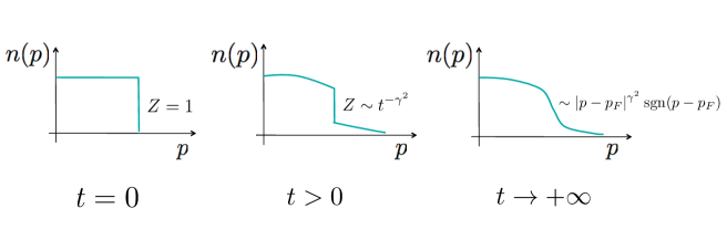
Figure 1: Schematic evolution of the momentum $n(p)$ distribution of the Luttinger model in the neighborhood of the Fermi momentum, $p_{F}$, following a quench of the interaction. The non-equilibrium exponent $\gamma^{2}=(K^{2}+K^{-2}-2)/4$, where $K$ is the Luttinger parameter, which parametrizes the correlations in the ground state, is different from the equilibrium exponent, $\gamma^{2}_{\mathrm{eq}}=(K+K^{-1}-2)/2$

In order to obtain the time evolution of correlations from the initial (non-interacting) state and study how the fermionic features of the non-interacting LM are wiped out, let us consider the instantaneous single-particle density matrix cazalilla2006 :

$$C_{\psi_{R}}(x,t)=\langle 0|e^{iH_{LM}t}\psi^{{\dagger}}_{R}(x)\psi(0)e^{-iH_{LM}t}|0\rangle=\langle 0|\psi^{{\dagger}}_{R}(x,t)\psi_{R}(0,t)|0\rangle,$$ (24)

which can be computed using the bosonization formula, Eq. (14), together with Eq. (21). The calculation proceeds pretty much along the lines of the calculation in the equilibrium case cazalilla2004 ; cazalilla_rmp ; giamarchi_book ; bosonization_new , and yields the following result in the scaling limit (i.e. for $d(x|L),d(2vt|L)\gg R$):

$$C_{\psi_{R}}(x,t) =Z(x,t)C^{(0)}_{\psi_{R}}(x),$$ (25)

$$Z(x,t) =\left[\frac{R}{d(x|L)}\right]^{\gamma^{2}}\left[\frac{d(x-2vt|L)d(x+2vt|L)}{d(2vt)}\right]^{\gamma^{2}/2},$$ (26)

Likewise, we can obtain the density correlations:

$$C_{\rho_{R}}(x,t) =\langle 0|e^{iH_{LM}t}\rho_{R}(x)\rho_{R}(0)e^{-iH_{LM}t}|0\rangle=\langle 0|\rho_{R}(x,t)\rho_{R}(0,t)|0\rangle$$ (27)

$$=-\frac{1}{4\pi}\left\{\frac{1+\gamma^{2}}{\left[d(x|L)\right]^{2}}-\frac{\gamma^{2}}{2\left[d(x-2vt|L)\right]^{2}}-\frac{\gamma^{2}}{2\left[d(x+2vt|L)\right]^{2}}\right\}.$$ (28)

In the avobe expressions $v=v(q=0)$ and $\gamma^{2}=\sinh^{2}\left(2\varphi(q=0)\right)=(K^{2}+K^{-2}-2)/4$, where $K=e^{2\varphi(q=0)}$ is the Luttinger parameter. Note that since the correlation functions are periodic functions of time and will exhibit periodic recurrences with a period $t_{L}=L/2v$. This is the consequence of the finite size of the system. In the thermodynamic limit, $L\to+\infty$, and therefore $t_{L}\to+\infty$. Thus, the cord functions yield power-laws by the replacement $d(z|L)\to|z|$.

For $L\to+\infty$ (or for $|x|,2vt\ll L$), the behavior of the above correlation functions exhibits two clearly distinct regimes. At short times, i.e. for $t\ll|x|/2v$,

$$C_{\psi_{R}}(x,t) \simeq Z(t)C^{(0)}_{\psi_{R}}(x),\quad Z(t)\sim t^{-\gamma^{2}}$$ (29)

$$C_{\rho_{R}}(x,t) \simeq-\frac{1}{4\pi^{2}x^{2}}=C^{(0)}_{\rho_{R}}(x).$$ (30)

That is, the correlations take a similar form to those of the non-interacting system. In the case of the single-particle density matrix, it decreases by an overall factor $Z(t)\sim t^{-\gamma^{2}}$. On the other hand, in the long time regime, i.e. for $t\gg|x|/2v$, the correlations crossover to

$$C_{\psi_{R}}(x,t) \simeq C^{(0)}_{\psi_{R}}(x)\left|\frac{R}{x}\right|^{\gamma^{2}},$$ (31)

$$C_{\rho_{R}}(x,t) \simeq-\frac{1+\gamma^{2}}{4\pi^{2}x^{2}}.$$ (32)

In this case, the correlations become qualitatively different from the initial state correlations. In particular, to leading order, they do not depend on time, which indicates that for $t\to+\infty$ the system reaches a steady state. We shall investigate this behavior more in detail further below, in section V. However, at this point, it is worth pointing out that the existence of the two distinct correlation regimes separated by a time scale $t_{x}=|x|/2v$ has to do with the finite propagation velocity of the elementary excitations of the LM. Since the LM is a relativistic model in which the role of the speed of light is played by the boson velocity $v$, this can be expected. The time scale $t_{x}$ is thus related to the time it takes for the excitations in the initial state localized at two points a distance $|x|$ apart to overlap. This phenomenon has been termed ’light-cone effect’ by Cardy and Calabrese cardycalabrese2006 in their study of quantum quenches starting from an off-critical state and ending in a critical state. In a more general framework, it is the consequence of the Lieb-Robison-type bounds liebrobinson for propagation of signals in systems with finite-range interactions.

The correlations in the steady state are different from those of the initial state and from those in the ground state of the LM. Despite the fact that the initial state is a complicated superposition of eigenstates of $H_{LM}$, the correlations are not thermal. If they were, they would exhibit an exponential decay beyond a characteristic length scale determined by the final (effective) temperature of the system $T_{f}$ (see e.g. cazalilla2004 ; cazalilla_rmp ; giamarchi_book ; bosonization_new and references). To see this, let us consider an “infinitesimal” quench in which an very weak interaction (i.e. $\varphi(q=0)\ll 1$) is switched on. Thus, the energy of the initial state differs from the energy of the LM ground state (taken to be zero) by an infinitesimal amount,

$$\frac{\Delta E}{L}=\frac{1}{L}\langle 0|H_{LM}|0\rangle =\frac{1}{L}\sum_{q\neq 0}v(q)|q|\langle 0|b^{{\dagger}}(q)b(q)|0\rangle\approx\frac{v}{\pi R^{2}}\sinh^{2}\varphi(q=0)\simeq\frac{v}{\pi R^{2}}\varphi^{2}(q=0),$$ (33)

which means that only low-lying excited states should be involved in the evolution following the quench. Thus, we can use the low-temperature form of the free energy in the canonical Gibbs ensemble for the LM (see e.g. Ref.mattislieb1965 ) $F(T)/L\simeq\pi^{2}T^{2}_{f}v/6$. Hence, the corresponding final temperature, $T_{f}\propto\varphi(q=0)$. However, this is still finite, which means that, if the system relaxes to the canonical Gibbs ensemble, the correlations should decay exponentially at long distances bosonization_new ; cazalilla2004 , e.g.:

$$C_{\psi_{R}}(x,t\to+\infty)\sim e^{-|x|/\xi(T_{f})},$$ (34)

for $|x|\gg\xi(T_{f})$ where $\xi(T_{f})\propto v/T_{f}$. By contrast, the asymptotic $t\to+\infty$ state following the quantum quench exhibits power-law correlations, as we have shown above. In other words, the system does not thermalize to the canonical Gibbsian ensemble. We will see in Sec. V that this is because the LM is exactly solvable and relaxes instead to a generalized Gibbs ensemble.

Before discussing the properties of the asymptotic state, let us discuss the consequences of the above results for the evolution of the momentum distribution. As discussed in Sec. II, the latter is the Fourier transform of the equilibrium single-particle density matrix. By analogy, we can define the instantaneous momentum distribution,

$$n(p,t)=\int dx\>e^{-ipx}C_{\psi_{R}}(x,t)=\left\{\begin{array}[]{cc}Z(t)\>\theta(p_{F}-p)&\text{for finite}\>t\quad(Z(t)\sim t^{-\gamma^{2}}),\\ \frac{1}{2}+\mathrm{sgn}(p-p_{F})|p_{F}-p|^{\gamma^{2}-1}&\mbox{for }t\to+\infty.\end{array}\right.$$ (35)

The results on the left-hand side hold for $p\approx p_{F}$. Fig. 1 shows the evolution of the momentum distribution schematically. The discontinuity at the Fermi momentum $p_{F}$ decreases algebraically and closes for $t\to+\infty$ becoming a weaker, power-law singularity, with an exponent that differs from the exponent characterizing the discontinuity at $p_{F}$ in the ground state.

Additional post-quench correlation functions were obtained by Iucci and Cazalilla in Ref. iucci2009 . We just quote here their results for the correlations of the so-called vertex operators starting from the non-interacting ground state. For the ratio of the non-equilibrium to the initial state correlations, the following results hold in the thermodynamic limit:

$$\frac{C_{V^{2m}_{\phi}}(x,t)}{C^{(0)}_{V^{2m}_{\phi}}(x)} =\frac{\langle 0|e^{2im\phi(x,t)}e^{-2im\phi(0,t)}|0\rangle}{\langle 0|e^{2im\phi(x)}e^{-2im\phi(0)}|0\rangle}=\mathcal{A}^{\phi}_{m}\left|\left(\frac{R}{2vt}\right)\left(\frac{x^{2}-(2vt)^{2}}{x^{2}}\right)\right|^{m^{2}(K^{2}-1)/2},$$ (36)

$$\frac{C_{V^{m}_{\theta}}(x,t)}{C^{(0)}_{V^{m}_{\theta}}(x)} =\frac{\langle 0|e^{im\theta(x,t)}e^{-im\theta(0,t)}|0\rangle}{\langle 0|e^{im\theta(x)}e^{-im\theta(0)}|0\rangle}=\mathcal{A}^{\theta}_{m}\left|\left(\frac{R}{2vt}\right)\left(\frac{x^{2}-(2vt)^{2}}{x^{2}}\right)\right|^{m^{2}(K^{-2}-1)/8},$$ (37)

where $m$ is an integer. In the above expressions cazalilla_rmp ; cazalilla2004 ; bosonization_new ; giamarchi_book ,

$$C^{(0)}_{V^{2m}_{\phi}}(x) =\langle 0|e^{2im\phi(x)}e^{-2im\phi(0)}|0\rangle=\left|\frac{R}{x}\right|^{2m^{2}},$$ (38)

$$C^{(0)}_{V^{m}_{\theta}}(x) =\langle 0|e^{im\theta(x)}e^{-im\theta(0)}|0\rangle=\left|\frac{R}{x}\right|^{m^{2}/4}.$$ (39)

Notice that the usual equilibrium duality relations requiring that if $\phi\to\theta$ then $K\to K^{-1}$ also hold for the post-quench correlations. Besides the above results, Iucci and Cazalilla also studied correlations at finite temperature, obtaining the momentum distribution in the asymptotic steady state at $t\to+\infty$. In Ref. iucci2009 , a quantum quench in which the interactions are suddenly switched off was also studied. We refer the interested reader to section II.-C of Ref. iucci2009 for the detailed form of the post-quench correlations in this case.

In the derivation of the previous results, it has been assumed that the interactions are long ranged but not singular. This translates into $g_{2}(q)$ and $g_{4}(q)$ being regular functions of $q$ as $q\to 0$, which is necessary to ensure that $K$ and $v$ are both finite. This is not the case for the Coulomb interaction for which $g_{2}(q)=g_{4}(q)=V(q)/2\pi$. Here $V(q)=2e^{2}K_{0}(qd)$ is the Fourier transform of the Coulomb potential, $K_{0}(x)$ being the modified Bessel function and $d$ a length scale of the order of the transverse dimensions system (recall that $K_{0}(x\ll 1)=\log\left(\frac{2}{xe^{\gamma}}\right)+\cdots$, where $\gamma=0.5772156649\ldots$ is Euler’s constant). The post-quench correlations for the LM with Coulomb interactions have been obtained by Nessi and Iucci nessi2013 . In what follows, we reproduce here their results for the single-particle density matrix, specializing to the case of a quench from the non-interacting system (which corresponds to setting $K_{i}=1$ in their expressions). For the single-particle density matrix $C_{\psi_{R}}(x,t)$, the following expression for the factor $Z(x,t)$ in Eq. (25) was obtained nessi2013 :

$$Z(x,t) =\exp\left\{-\int^{+\infty}_{0}\frac{dq}{q}\>\sinh^{2}\left[\varphi(q)\right]\left[1-\cos\left(2v(q)qt\right)\right]\left(1-\cos qx\right)\right\},$$ (40)

where $v(q)=\sqrt{v_{F}(v_{F}+2V(q)/\pi)}$ is the Tomonaga boson velocity, $v(q\ll 1/d)\sim v_{F}\log^{1/2}(1/qd)$; the Bogoliugov rotation angle of the LM in the presence of Coulomb interactions follows from $\tanh 2\varphi(q)=V(q)/(2\pi v_{F}+V(q))$. Asymptotic expressions can be obtained from Eq. (40). For instance, the asymptotic long time limit reads nessi2013 :

$$C_{\psi_{R}}(x,t\to+\infty)=C^{(0)}_{\psi_{R}}(x)e^{-\frac{g}{4}\log^{2}(x/d)},$$ (41)

where $g=e^{2}/\pi v_{F}$, $e$ being the fundamental fermion charge. This form again differs from the equilibrium expression giamarchi_book ; nessi2013 . The intermediate time dynamics, however, is complicated by the divergence of the Tomonaga boson velocity $v(q)$ as $q\to 0$, which leads to a non-linear light-cone effect nessi2013 . Thus, for times fulfilling the condition:

$$\frac{d}{v_{F}}\ll t\ll t_{x}=\frac{x}{2v_{F}\sqrt{1+2g\log(d/x)}},$$ (42)

the single-particle density matrix takes the form:

$$C_{\psi_{R}}(x,t)=C^{(0)}_{\psi_{R}}(x)e^{-\frac{g}{4}\log^{2}(2v_{F}t/d)}$$ (43)

with exponential accuracy. Hence, it follows that the discontinuity at $p_{F}$ in momentum distribution decreases as $Z(t)\sim e^{-\frac{g}{4}\log^{2}(2v_{F}t/d)}$ instead of the power-law $\sim t^{-\gamma^{2}}$ found for the LM with non-singular interactions. Asymptotic forms for other post-quench correlations, such as those of vertex operators, were also obtained in Ref. nessi2013 , and we refer the interested reader to the original article for the details.

III.3 Quest for universality: Quenches in models of the TLL class

In the previous subsection, we have reviewed the results obtained for a sudden quench of the interaction in the LM. Since sudden quenches can potentially drive the system far from equilibrium, there is no reason to expect that the results discussed above can be universal. Indeed, universality applies to the low-temperature, long distance and time correlations of systems in equilibrium and it is borne out on the ideas of the renormalization group rg_shankar ; rg_book . According to the latter, the low-temperature properties of a system are rather insensitive to the microscopic details as it is the structure of the low-lying excited states. Therefore, a sudden quantum quench that involves highly excited states is not likely to yield correlations that are universal.

Nevertheless, since LM is a renormalization-group fixed point for the Tomonaga-Luttinger liquid universality class, there is much interest in investigating to which extent correlations following a sudden quench exhibit universality. Analytical progress in this regard is particularly difficult. Therefore, in order to ascertain whether the correlations are independent or not of the microscopic details of the model, a number of numerical and semi-numerical techniques have been deployed.

In particular, the LM prediction for the dynamics of the discontinuity at $p_{F}$ in the momentum distribution reviewed in the pervious section, has been numerically tested by Karrasch, Rentrop, Schuricht, and Meden (KRSM) karraschmedem2012 using time-dependent DMRG tddmrg . KRSM considered a (sudden) quench of the interaction in the following lattice model:

$$H=\sum_{m=1}^{L}\left[-\frac{1}{2}\left(c^{{\dagger}}_{m+1}c_{m}+c^{{\dagger}}_{m}c_{m+1}\right)+\sum_{m}\left(\Delta n_{m}n_{m+1}+\Delta_{2}n_{m}n_{m+2}\right)\right],$$ (44)

from the non-interacting system, i.e. starting from the ground state of the XX model (i.e. $\Delta=\Delta_{2}=0$) to the interacting model with either $\Delta\neq 0$ or $\Delta\neq 0$ and $\Delta_{2}\neq 0$. In the former case, the model is known as the XXZ model and it can be solved exactly using the Bethe-ansatz method (see e.g. giamarchi_book ; cazalilla_rmp and references therein). However, when the term proportional to $\Delta_{2}$ is present, the model is no longer integrable in Bethe-ansatz sense. Yet, the results in both cases showed good agreement with the LM predictions.

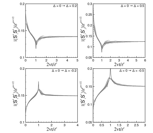
Figure 2: Scaled transverse spin correlations ($\langle S^{x}_{i}(t)S^{x}_{j}(t)\rangle$) for a sudden quench of the anisotropy ($=$ interaction) in the Heisenberg-Ising (XXZ) spin chain obtained using the TEBD algorithm tddmrg in Ref. collura2015 . The correlations are scaled by a factor of $\ell^{\alpha+1/2}$, where $\ell=i-j$ and plotted vs. $2vt/\ell$ ($v$ is the spinwave velocity and $t>0$ is time); the exponent $\alpha=(K^{-2}-1)/4$, where the Luttinger parameter $K<1$ for $\Delta>0$ ($K>1$ for $\Delta<0$), is determined from the Bethe-ansatz solution of the XXZ model $K=\frac{1}{2}\left[1-\frac{1}{\pi}\cos^{-1}\left(\Delta\right)\right]^{-1}$  cazalilla_rmp ; giamarchi_book ; bosonization_new ; collura2015 . The Luttinger model prediction (dashed line) (cf. Eqs. 37 and 46) is $|\langle S^{x}_{i}(t)S^{x}_{j}(t)\rangle|\ell^{\alpha+1/2}\sim t^{-\alpha}\left[1-(2vt/\ell)^{2}\right]^{\alpha}$. In addition to the scaling predicted by the LM, the plot also shows the the light-cone effect appearing as a cusp (rounded off by short-distance lattice effects) at $2vt/\ell\simeq 1$.

In addition, KRSM also obtained the evolution of the kinetic energy per unit length, i.e.

$$e_{\mathrm{imp}}(t)=-\frac{1}{2L}\sum_{m=1}^{L}\langle\Phi_{0}|e^{iHt}\left(c^{{\dagger}}_{m+1}c_{m}+c^{{\dagger}}_{m}c_{m+1}\right)e^{-iHt}|\Phi_{0}\rangle,$$ (45)

where $|\Phi_{0}\rangle$ is the ground state of the non-interacting model (i.e. Eq. 44 with $\Delta=\Delta_{2}=0$). The time-derivative kinetic energy exhibits a universal power-law decay $\sim c(K,v)/t^{3}$ whose prefactor $c(K,v)=(K^{2}+K^{-2}-2)v_{F}/16\pi v^{2}$ karraschmedem2012 ; nessi2013 is a function of the Luttinger parameter $K$ and the Tomonaga-boson velocity, $v$ , which provides a further test for the universality of the LM predictions.

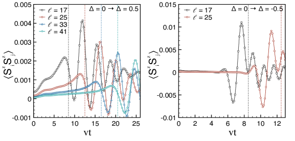
Figure 3: Longitudinal spin correlation function $\langle S^{z}_{i}S^{z}_{j}\rangle$ as function of $vt$ for several separations $\ell=j−i$, for a sudden quench of the anisotropy ($=$ interaction) in the Heisenberg-Ising (XXZ) spin chain computed numerically using the TEBD algorithm tddmrg in Ref. collura2015 . As the light-cone is approached (corresponding to the vertical dashed lines for different values of $\ell$) $t\gg|x|/v=\ell/v$, namely $\ell^{-\alpha-1}$. The oscillations are not predicted by the Luttinger model.

More recently, a thorough study of the universality (and lack thereof) of the LM predictions has been undertaken by Collura, Calabrese, and Essler (CCE) collura2015 . These authors carried out a numerical study of a suddent quench in XXZ spin chain (cf. Eq. 44 with $\Delta_{2}=0$, see also Eq. (65) below for the model in terms of spins). CCE analyzed quenches starting from the ground state with the XX model ($\Delta=0$) and considered several values for the Ising coupling in the post-quench Hamiltonian $\Delta=\pm 0.2,\pm 0.5$. Using the time-evolving block decimation (TEBD) algorithm tddmrg , they numerically obtained the transverse and longitudinal spin-spin correlations, for which (to leading order) the LM predictions are:

$$\langle S^{x}_{n+\ell}(t)S^{x}_{n}(t)\rangle \simeq(-1)^{|\ell|}\>C_{V^{1}_{\theta}}(x=\ell a_{0},t),$$ (46)

$$\langle S^{z}_{n+\ell}(t)S^{z}_{n}(t)\rangle \simeq 2C_{\rho_{R}}(x=\ell a_{0},t)+(-1)^{|\ell|}C_{V^{2}_{\phi}}(x=\ell a_{0},t).$$ (47)

where $a_{0}$ is the lattice parameter, and $C_{V^{m=1}_{\theta}}(x,t)$, $C_{\rho_{R}}(x,t)$ and $C_{V^{2m=2}_{\phi}}(x,t)$ are given by Eqs. (37), (36), and (28), respectively. CCE found a fairly good agreement of the LM predictions with the numerics for the transverse spin correlations, $\langle S^{x}_{i+l}(t)S^{x}_{i}(t)\rangle$ (see Fig. 2). However, the agreement with the LM predictions for the longitudinal correlations, $\langle S^{z}_{i+l}(t)S^{z}_{i}(t)\rangle$, was found to be much poorer (see Fig. 3). CCE convincingly argued that the lack of agreement in the latter case stems from the different character of the $S^{z}_{n}$ spin operators, as compared to $S^{x}_{n}$. Indeed, the spin operator measuring the projection on the $z$-axis reads: bosonization_new ; giamarchi_book :

$$S^{z}_{n}=c^{{\dagger}}_{n}c_{n}-\frac{1}{2}\simeq\frac{1}{\pi}\partial_{x}\phi(x=na_{0})+(-1)^{n}\cos 2\phi(x=na_{0})+\cdots$$ (48)

that is, a rather local operator in terms of the Jordan-Wigner fermion operators $c_{n}$ and $c^{{\dagger}}_{n}$ giamarchi_book ; cazalilla_rmp . On the other hand, the spin operator along the $x$ axis,

$$S^{x}_{n}=(c_{n}+c^{{\dagger}}_{n})\prod_{l<n}\left(1-2c^{{\dagger}}_{l}c_{l}\right)=(-1)^{n}\cos\theta(x=na_{0})+\cdots,$$ (49)

is rather non-local operator due to the Jordan-Wigner string $\prod_{l<n}\left(1-2c^{{\dagger}}_{l}c_{l}\right)$ giamarchi_book ; cazalilla_rmp . To fully appreciate the impact of this difference, let us recall that the (initial) state, which is the ground state of the XX model (i.e. $\Delta=0$), can be written as a non-interacting Fermi sea of the Jordan-Wigner fermions, i.e. $|0\rangle=\prod_{k<\frac{\pi}{2}}c^{{\dagger}}_{k}|\mathrm{vac}\rangle$, where $|\mathrm{vac}\rangle$ is the Fermion vacuum state and $c_{k}=L^{-1}\sum_{n}e^{-ikn}c_{n}$.

III.4 Pre-thermalization and quench in a 2D Fermi liquid

Pre-thermalization was discussed by Berges and coworkers in the context of high-energy ion collisions berges . It refers to metastable state of a system that has been driven out of equilibrium rapidly establishes a kinetic temperature based on the average kinetic energy. Despite this fact, the eigenmode distribution of the in the metastable state does not correspond to a Bose-Einstein (for bosons) or a Fermi-Dirac (for fermions) distribution. These ideas have found resonance in the study of non-equilibrium (quench) dynamics of ultracold atomic systems. Moeckel and Kehrein moeckel2008 discussed them in relation to a two-stage thermalization scenario that should take place following a quantum quench. In their work, Moeckel and Kehrein studied a quench of the interaction in the Hubbard model using the flow equation method moeckel2008 . Considering the infinite-dimensional Hubbard model on the Bethe lattice, they obtained the short to intermediate time evolution of the momentum distribution. Their result shows some striking resemblance with the results described earlier for the LM (cf. Fig. 1). However, one major difference with the LM is that the discontinuity at the Fermi surface does not close completely. Instead, Moeckel and Keherein found that it saturates at a constant value $Z_{\mathrm{neq}}$ which obeys the relation $(1-Z_{\mathrm{neq}})=2\left(1-\mathrm{Z}_{\mathrm{eq}}\right)$, where $Z_{\mathrm{eq}}<1$ is the discontinuity in the momentum distribution in the interacting ground state.

Pre-thermalization has also been discussed in connection to study of quantum quenches in ultracold bosonic gases in Schmiedmayer’s group in Viena  pretherm1 ; pretherm2 . However, in this section, we focus on reviewing the results for the pre-thermalization dynamics for a two-dimensional (2D) gas of spinless fermions interacting with long-ranged interactions, which, in a certain sense, can be regarded as the 2D generalization of the LM. The dynamics ensuing a quench of the interaction in this system has been studied by Nessi, Iucci, and Cazalilla (NIC) nessi2014 , and it may be of relevance for the study of the non-equilibrium dynamics of dipolar quantum gases dipolar_fermigases . The Hamiltonian of the model studied by NIC reads:

$$H =H_{0}+H_{\mathrm{int}},$$ (50)

$$H_{0} =\sum_{k}\epsilon(\boldsymbol{k})\psi^{{\dagger}}(\boldsymbol{k})\psi(\boldsymbol{k}),$$ (51)

$$H_{\mathrm{int}} =\frac{1}{2\Omega}\sum_{\boldsymbol{k}\boldsymbol{p}\boldsymbol{q}}V(\boldsymbol{q})\psi^{{\dagger}}(\boldsymbol{k}+\boldsymbol{q})\psi^{{\dagger}}(\boldsymbol{p}-\boldsymbol{q})\psi(\boldsymbol{p})\psi(\boldsymbol{q}),$$ (52)

where $\psi(\boldsymbol{k})$ ($\psi^{{\dagger}}(\boldsymbol{k})$) annihilate (create) fermions with momentum $\boldsymbol{k}$, where $\boldsymbol{k}=(k_{x},k_{y})$ is a two dimensional vector. As in the case of the LM, it was assumed by NIC that the system is prepared in the ground state of the non-interacting Hamiltonian $H_{0}$ and it evolves according to the interacting Hamiltonian $H$ for $t\geq 0$, which is tantamount to a quench of the interaction. The Fourier transform of interaction potential $V(\boldsymbol{q})$ is assumed to vanish rapidly for $|\boldsymbol{q}|\gg q_{c}$, where $q_{c}\sim R\gg p^{-1}_{F}$, $R$ being the range of the interaction and $p_{F}=\sqrt{4\pi\rho_{0}}$ the Fermi momentum ($\rho_{0}$ is the areal particle density). In order to render the expressions analytically tractable, the Fourier transform of the interaction potentila is taken of to be of form $V(\boldsymbol{q})=f_{0}\,(q/q_{c})^{n}e^{-q/q_{c}}$, where $f_{0}$ parametrizes the interaction strength and $n=0,1,\ldots$ is a positive or zero integer (see below).

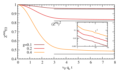
Figure 4: Time-evolution of the discontinuity at the Fermi momentum following an quench of the interaction in a two-dimensional Fermi liquid with long range interactions nessi2014 . The short time behavior is $Z(t)\simeq 1-ct^{2}$, where $c\propto f^{2}_{0}$, where $f_{0}$ is the strength of the interaction. The inset shows better detail of the way $Z(t)$ approaches its constant asymptote as $t^{-1}$. The dimensionless inteaction coupling $g=f_{0}\sqrt{p_{F}q_{c}/2\pi^{2}v_{F}}$. The horizontal lines indicate the long-time pre-thermal asymptote, $Z_{\mathrm{neq}}=(Z_{\mathrm{eq}})^{2}$, which is obtained from the Fermi-surface bosonization treatment (cf. section III.4).

To access the short to intermediate time dynamics of the model, NIC first carried out a perturbative analysis to leading (i.e. second) order in the interaction. Thus, they showed that, the discontinuity at $p_{F}$ of the momentum distribution, $Z(t)$, also exhibits a plateau similar to the one observed by Moeckel and Kehrein moeckel2008 in the case of the Hubbard model (see also Eckstein et al. eckstein2009 ). This plateau indicates the existence of a pre-thermalized state. Furthermore, NIC found that, to the leading order in $f_{0}$, the relationship $1-Z_{\mathrm{neq}}=2(1-Z_{\mathrm{eq}})$ also holds for the 2D Fermi gas described by the above model.

In addition, in order to understand the emergence of the pre-thermalized state, NIC resorted to the Fermi surface (FS) bosonization method FSbosonization . This method has been applied in equilibrium and it provides a non-perturbative foundation to Landau’s Fermi liquid theory. Unlike the equilibrium case where the method is applied to a low-energy effective Hamiltonian FSbosonization , NIC applied it to the bare Hamiltonian, $H$ (cf. Eq. 50), which describes the interactions between the bare fermions. Performing a truncation of $H$ that amounts to neglecting inelastic scattering between the fermions and keeps only forward and exchange interactions, NIC nessi2014 re-wrote $H$ in terms of the Fourier components of the density operator FSbosonization :

$$H\simeq\sum_{\boldsymbol{S},\boldsymbol{T}}\sum_{|\boldsymbol{q}|\ll\lambda}\rho_{\boldsymbol{S}}(\boldsymbol{q})\left[\frac{v_{F}}{\Omega}+\frac{V(\boldsymbol{q})}{A}\right]\rho_{\boldsymbol{T}}(-\boldsymbol{q}),$$ (53)

where $v_{F}=|\boldsymbol{\nabla}_{\boldsymbol{k}}\epsilon(\boldsymbol{k})|$ is the Fermi velocity and $A$ is the area of the system. In writing Eq. (53), it is assumed that a crown of width $\lambda$ around the FS has been “sectorized” into $N$ squat patches of transverse size $\Lambda$, such that $p_{F}\gg\Lambda\gg\lambda>q_{c}$ . The constant $\Omega=\Lambda A/(2\pi)^{2}$. As in the case of TLLs, the Fourier components of the density, $\rho_{\boldsymbol{S}}(\boldsymbol{q})$ obey a KM algebra FSbosonization ($|\boldsymbol{q}|,|\boldsymbol{q}^{\prime}|\ll\lambda$, compare with Eq. 5):

$$\left[\rho_{\boldsymbol{S}}(\boldsymbol{q}),\rho_{\boldsymbol{T}}(\boldsymbol{q^{\prime}})\right]=\Omega\left(\boldsymbol{q}\cdot\boldsymbol{\hat{n}}_{\boldsymbol{S}}\right)\delta_{\boldsymbol{S},\boldsymbol{T}}\delta_{\boldsymbol{q}+\boldsymbol{q^{\prime}},\boldsymbol{0}},$$ (54)

where $\boldsymbol{\hat{n}}_{\boldsymbol{S}}$ is a unit vector normal to the circular FS at the patch position of $\boldsymbol{S}$. This equation turns the diagonalization of Eq. (53) into a problem akin to a system of (chiral) Luttinger models (one for each FS patch) coupled by forward-scattering interaction. Like in the case of the LM, the KM algebra allows us to obtain a diagonal representation of Eq. 54 in terms of a set of bosonic eigenmode operators:

$$H\simeq\sum_{l,\boldsymbol{q}}\omega_{l}(q)b^{{\dagger}}_{l}(\boldsymbol{q})b_{l}(\boldsymbol{q}).$$ (55)

This expressions clearly shows that the short to intermediate-time dynamics described by $H$ can be approximated by a exactly solvable Hamiltonian, whose dynamics is strongly constrained by the integrals of motion $I_{l}(\boldsymbol{q})=b_{l}(\boldsymbol{q})b_{l}(\boldsymbol{q})$ (more on this further below).

In addition, the diagonalization of $H$ (neglecting inelastic scattering between fermions) allowed NIC to obtain non-perturbative results for the evolution of the post-quench single-particle density matrix. Using similar expressions to the bosonization formula, Eq. (14) FSbosonization , the following results for the behavior of the discontinuity in the momentum distribution at the FS were obtained nessi2014 :

$$Z(t\ll R/v_{F}) =\exp\left[-ct^{2}\right],$$ (56)

$$Z(t\gg R/v_{F}) =Z_{\mathrm{neq}}e^{g^{2}a_{n}(v_{F}q_{c}t)^{-(2n+1)}}.$$ (57)

where $c$ depends on the details of the interaction nessi2014 and $g=f_{0}\sqrt{p_{F}q_{c}/2\pi^{2}v_{F}}$. The long-time asymptote of $Z(t)$ obeys $Z_{\mathrm{neq}}=(Z_{\mathrm{eq}})^{2}$, which is the non-perturbative version of Moeckel and Kehrein’s relationship between the equilibrium and pre-thermalized values of the discontinuity at $p_{F}$ moeckel2008 . The full crossover from the short time limit (which agrees with the perturbative results nessi2014 ) to the long time limit of Eq. (57) was obtained by evaluating the integrals numerically and it is shown in Fig. 4.

Thus, the explicit construction of the exactly solvable truncation of $H$ gives access to a non-perturbative solution of the short to intermediate time dynamics (up to times $t\gtrsim f^{2}_{0}N(0)$ ($N(0)=k_{F}/2\pi v_{F}$ being the density of states at the Fermi level), at which inelastic collisions kick in and should drive the system to a thermal state. In addition, it also clarifies the physical origin of the phenomenon of pre-thermalization by relating it to constrained dynamics of the exactly solvable model of Eq. (55), which is as we will exactly in section V relaxes not to the grand canonical ensemble, but to the generalized Gibbs ensemble due to the combination of Gaussian nature of the initial state and the dephasing between the bosonic FS eigenmodes of (55).

IV Smooth quantum quenches

IV.1 Analytical results

In the previous section, we have focused on the dynamics following a sudden quench of the interaction. However, both from the theoretical and experimental point of view, it is interesting to consider the question of how the system may evolve under a smooth quench. In the case of the LM, it allows to study the non-equilibrium dynamics of the system as a function of the rate with which the interaction is turned on, sudden quenches corresponding to the the fastest rate and the adiabatic limit to the slowest one. Therefore, the study of the smooth quenches can be used to compare the effects of a sudden quench to an adiabatic evolution and to better understand the mechanisms by which quantum many-body systems are driven out of equilibrium. In addition, time scale which controls the change in the Hamiltonian parameters the non-equilibrium dynamics with the question how it compares to other characteristic time scales of the problem is an important input for experiments studying quench dynamics.

Another interesting question that can be addressed in this context is how much the time-evolved state of the system is reminiscent of the original starting state. In this regard, the Loschmidt echo, or fidelity in the quantum information-theoretic language, measures the overlap between the state of the smoothly quenched system and the initial state. This measurement provides direct insight into the many-body dynamics and the relation between quench dynamics and quantum information.

For a smooth-quench the Hamiltonian becomes explicitly time-dependent:

$$H(t)=\sum_{q\neq 0}\left\{\omega(q,t)a^{\dagger}(q)a(q)+\frac{1}{2}g_{2}(q,t)|q|\left[a(q)a(-q)+a^{\dagger}(q)a^{\dagger}(-q)\right]\right\}.$$ (58)

where $\omega(q,t)=\left[v_{F}+g_{4}(q,t)\right]|q|$. The time evolution is described by the Heisenberg equation of motion:

$$i\partial_{t}a(q,t)=[a(q,t),H(t)]=\omega(q,t)a(q,t)+g_{2}(q,t)|q|a^{\dagger}(-q,t),$$ (59)

and similarly

$$i\partial_{t}a^{\dagger}(-q,t)=-\omega(q,t)a^{\dagger}(-q,t)-g_{2}(q,t)|q|a(q,t).$$ (60)

This equation of motion can be solved by a similar ansatz to the one used for the sudden quench:

$$a(q,t)=f(q,t)a(q)+g^{\star}(q,t)a^{\dagger}(-q).$$ (61)

However, in this case the functions $f(q,t)$ and $f(q,t)$ obey the Bogoliubov-deGennes (BdG) equations of motion:

$$i\partial_{t}\left[\begin{matrix}f(q,t)\\ g(q,t)\end{matrix}\right]=\left[\begin{matrix}\omega(q,t)&g_{2}(q,t)|q|\\ -g_{2}(q,t)|q|&-\omega(q,t)\end{matrix}\right]\left[\begin{matrix}f(q,t)\\ g(q,t)\end{matrix}\right],$$ (62)

which are supplemented by the initial conditions: $f(q,0)=1$ , and $g(q,0)=0$ and the constraint $|f(q,t)|^{2}-|g(q,t)|^{2}=1$, which is required by Bose-Einstein statistics. Thus, $f(q,t),g(q,t)$ contain all the dynamical information about the smooth quench and, as in the case of the sudden quenches, expectation values of the time-dependent observables can be obtained from their knowledge.

Dora, Haque and Zaránd (DHZ) DoraHaqueZarand obtained solutions to the BdG equations for a linear ramp of the the interaction assuming that $\omega(q,t)=\omega(q)=v_{0}(q)|q|$ is independent of time and

$$g_{2}(q,t)=g_{2}(q)Q(t)$$ (63)

where $Q(t)=t\Theta(t(t-\tau))/\tau+\Theta(t-\tau)$, with $\Theta(t)$ the Heaviside function. Note that $Q(t>\tau)=1$ and $Q(t<0)=0$, that is, $\tau$ determines the characteristic quench time. For $\tau\rightarrow 0$, a sudden quench is obtained, while the adiabatic limit is approached by letting $\tau\rightarrow\infty$. Assuming a perturbatively small $g_{2}(q)=g_{2}e^{-|q|R/2}$, DHZ obtained the following asymptotic form for the instantaneous single-particle density matrix (cf. Eq. 24) for $t\gg\tau$:

$$\frac{C_{\psi_{R}}(x,t)}{C_{\psi_{R}}^{(0)}(x)}\sim\left\{\begin{matrix}A\left(\frac{\tau}{\tau_{0}}\right)\left(\frac{R}{\min{(|x|,2v_{0}t})}\right)^{\gamma_{SQ}}&\mbox{for}\,|x|\gg 2v_{0}\tau\\ \left(\frac{R}{|x|}\right)^{\gamma_{ad}}&\mbox{for}\,|x|\ll 2v_{0}\tau\end{matrix}\right.$$ (64)

where $\gamma_{SQ}=g_{2}^{2}(q=0)/v_{0}^{2}+O(g^{3}_{2})$ and $\gamma_{ad}=g_{2}^{2}/2v_{0}^{2}+O(g^{3}_{2})$ ($v_{0}=v_{0}(q=0)$) are the (perturbative) sudden quench and adiabatic-limit exponents. The prefactor $A(\tau/\tau_{0})$ depends on the speed of the quench: For a sudden quench, $A(\tau/\tau_{0}\ll 1)\sim 1$, while for smooth quench $A(\tau/\tau_{0}>1)\sim(\tau/\tau_{0})^{\gamma_{ad}}$. The physical explanation for two kinds of behavior displayed in Eq. (64) lies in the following crossover behavior: When the interaction is quenched at a rate $\sim\tau^{-1}$, the “slow” excitations of energy $\omega(q)<\tau^{-1}$ experience it as a sudden quench. On the other hand, fast excitations with energies $\omega(q)>\tau^{-1}$ can adjust the the change of the interaction strength adiabatically. Since high (low) energy excitations determine the short (long) distance correlations, the tail of $C_{\psi_{R}}(x,t)$ is governed by the sudden quench exponent, whilst its short distance behavior is described by the adiabatic exponent.

The subject of smooth quenches has often been related to the dynamics across critical points (see e.g. KZMReview and references therein). However, for the quench of interaction in LM only one phase (critical) is involved. For example, for the XXZ model, only the critical region is related to the LM, and for Bose Hubbard models, LM corresponds to the superfluid regime. Therefore, the Kibble Zurek mechanism, which is related to the production of topological defects when quenching a system across a critical point, is not relevant for smooth quenches of the interaction in the LM. Nevertheless, it is possible to discuss the production of quasi-particles in a smooth quench of the interaction, as it was done by Dziarmaga and Tylukti Dziarmaga . The average density of excited quasiparticles $n_{ex}$ scales with $\tau$ as $n_{ex}\sim\tau^{-1}$, while the more directly measurable excitation energy density scales like $\varepsilon\sim\tau^{-2}$ at zero temperature. On the other hand, at finite temperature $\varepsilon\sim\tau^{-1}$. At zero temperature, Dziarmaga and Tylukti also showed that the production of excitations does not change the algebraic $x^{-2}$ decay of the density (cf. Eq. 32). Instead (relative to the initial state), they only yield an additive correction to the prefactor. This behavior contrast with the exponential decay of the correlations induced by the Kibble-Zurek mechanism following a quench from a disorder to an ordered phase.

IV.2 Comparison to numerical approaches

As in the case of sudden quenches, the LM predictions for the correlation functions and other quantities (see below) in the case of a smooth quench have been compared to numerical calculations. In this section, we review some of the most important results in this regard.

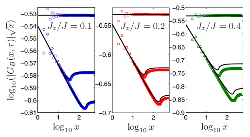
Figure 5: Post-quench spin-flip correlation function for $J_{z}/J=0.1$ (left panel), $0.2$ (middle panel), and $0.4$ (right panel) for $J\tau=0$, $20.2$ and $108.3$ (from top to bottom) compared with the Luttinger model prediction of Eq. (66). At short distances, the numerical results are influenced by lattice effects, and therefore deviate from the Luttiger model predictions.

In order to test the correctness of the LM predictions for smooth quench dynamics, Pollmann, Haque and Dóra (PHD) numerically studied the anisotropic (XXZ) Heisenberg model in the critical regime by using the infinite time-evolving block decimation algorithm (iTEDB) tddmrg . They considered the Hamiltonian:

$$H_{XXZ}=\sum_{m}\left[\left(S_{m}^{x}S_{m+1}^{x}+S_{m}^{y}S_{m+1}^{y}\right)+J_{z}(t)S_{m}^{z}S_{m+1}^{z}\right],$$ (65)

assuming antiferromagnetic exchange interaction, i.e. $J>0$ and quenching the Ising exchange, $J_{z}(t)$ according to $J_{z}(t)=J_{z}Q(t)$ with $Q(t<\tau)=t/\tau$ and $Q(t>\tau)=1$. As explained in section III.3, using the Jordan Wigner transformation (see e.g. Refs. bosonization_new ; giamarchi_book ; cazalilla_rmp ) this model can be mapped to an interacting lattice model of spinless fermions in 1D (cf. Eq. 44 with $\Delta_{2}=0$). Bosonization bosonization_new ; giamarchi_book then allows to relate this model to a smooth quench in the LM (cf. 58) with $\omega(q)=v|q|$ ($v=J$) and $g_{2}(q,t)=g_{2}(q)Q(t)$, $g_{2}(q)=g_{2}e^{-|q|R/2}$, being $R\sim a_{0}$ a short-distance cut-off of the order of the lattice parameter $a_{0}$. $R$ was numerically obtained by PHD to be $R=0.5622a_{0}$. In addition, the value of $g_{2}$ is fixed using perturbation theory, which requires that $-1\ll g_{2}/2J=J_{z}/\pi J\ll 1$.

The staggered part of the transverse magnetization is given by Eq. (49). Hence, in the scaling limit where $|x|,v\tau\gg R$ after the quench at $t=\tau$, the transverse post-quench correlations can be evaluated using bosonization to yield:

$$C_{S^{+}}(x,\tau)\approx\frac{C(-1)^{|x|}}{\sqrt{|x|}}\left|\frac{R}{x}\right|^{\frac{g_{2}}{2v}}\exp{\left[-\frac{g_{2}}{2v}f\left(\frac{x}{2v\tau}\right)\right]}$$ (66)

where $f(y)=1/2\sum_{s=\pm 1}s(y-s)\log|y-s|$, and $C=2^{-1/3}e^{1/2}A^{-6}$, where $A=1.28243\dots$ is Glaisher’s constant. In Fig.5, the comparison of this analytical result with the numerics from iTEDB is shown. The agreement is excellent for small $J_{z}/J$, although it worsens slightly for higher values of $J_{z}$.

In addition to correlation functions, Dora, Pollmann, Fortágh and Zaránd (DPFZ) have studied the Loschmidt echo (LE) LE as a many-body generalization of the orthogonality catastrophe anderson_oc . The LE is defined as the overlap of two wave functions $|\Psi_{0}(t)\rangle$ and $|\Psi(t)\rangle$ evolved from the same initial state $|\Psi_{0}\rangle$ but with different Hamiltonian ($H_{0}$ and $H$):

$${\cal L}(t)=\mid\langle\Psi_{0}\mid e^{iH_{0}t}e^{-iHt}\mid\Psi_{0}\rangle\mid^{2}.$$ (67)

In quantum information theory this quantity is also called fidelity , and it is a measure of the distance between two quantum states which can be used to identify irreversibility and chaos. Moreover, like entanglement measures, this quantity can be used to detect quantum phase transitions (see e.g. review_polkovnikov ; fidelity_qpt and references therein).

In their paper on LE, DPFZ considered a quench between two different values of the interaction, which corresponds to setting $g_{2}(q,t)=g_{i}(q)+\Delta g(q,t)$ in Eq. (58). Here $g_{i}(q)$ is the initial value of the interaction, $\Delta g(q,t)=[g_{f}(q)-g_{i}(q)]Q(t)$ (where $Q(t)$ has been defined above for a linear ramp of the interaction), and $g_{f}(q)$ is the final value of the interaction. The initial and final quasi-particle spectra are given by $\omega_{i(f)}(q)=\sqrt{\omega^{2}(q)-g_{i(f)}^{2}(q)q^{2}]}$, and the Luttinger parameters are characterized by those interaction strengths in the following way:

$$K_{i(f)}=\sqrt{\frac{\omega(q)-g_{i(f)}(q)|q|}{\omega(q)+g_{i(f)}(q)|q|}}.$$ (68)

Thus, DPFZ expressed the LE analytically in terms of the Bogoliubov coefficients of Eq. (62)):

$${\cal L}(t)=\exp{\left(-\sum_{q>0}\log{\left[\left|f(q,t)\right|^{2}\right]}\right)},$$ (69)

which expresses the LE in terms of the number of excited quasi-particles in the final state. Using $|f^{ad}(q,t)|^{2}=1/2+(K_{i}/K_{f}+K_{f}/K_{i})/4$ for $t>\tau$, DHPZ obtained for the the LE in the adiabatic limit the following expression fidelity :

$${\cal L}_{ad}=\left[\frac{1}{2}+\frac{1}{4}\left(\frac{K_{i}}{K_{f}}+\frac{K_{f}}{K_{i}}\right)\right]^{-\frac{L}{\pi a_{0}}},$$ (70)

were $L$ is the system size and and $a_{0}$ is the short-distance cut-off. Therefore, the LE decays exponentially with the system size, $L$.

On the other hand, for a sudden quench the long time limit of the LE takes a different form:

$${\cal L}_{SQ}\left(t\gg\frac{a_{0}}{2v_{0}}\right)={\cal L}_{ad}^{2}.$$ (71)

This can be understood in the following way: The LE of an adiabatic quench involves only the ground states of the initial and final Hamiltonian, i.e., square of the overlap of the ground states $\langle G|G_{0}\rangle$ where $|G_{0}\rangle$($|G\rangle$) is the ground state of $H_{0}$($H$). For a sudden quench, inserting the resolution of the identity operator in terms the eigenstates of the post quench Hamiltonian $H$ between the two evolution operators in $\langle\Psi_{0}|e^{iHt}e^{-iH_{0}t}|\Psi_{0}\rangle$, and after taking into account the dephasing of the energy phase factors of different excited states the ground state contribution remains. Asymptotically in the thermodynamic limits $|\langle\Psi_{0}|e^{iHt}e^{-iH_{0}t}|\Psi_{0}\rangle|=|\langle G|G_{0}\rangle|^{2}$. Hence, ${\cal L}_{SQ}=|\langle\Psi_{0}|e^{iHt}e^{-iH_{0}t}|\Psi_{0}\rangle|^{2}=|\langle G|G_{0}\rangle|^{4}={\cal L}_{ad}^{2}$ for $t\rightarrow\infty$. These results for the LE were numerically confirmed by DPFZ for the XXZ spin-chain model using matrix-product states DMRGBook .

Considering on a smooth quench of the interaction in a 1D Bose gas which can be described as a TLL cazalilla_rmp , Bernier and coworkers addressed the question how the system is driven out of equilibrium by an increasing quench rate Orignac . Working in the weakly interacting limit, where $v(t)K(t)$ remains time-independent and $u(t)/K(t)=(v_{0}/K_{0})(1+\tau/\tau_{0})$ ($\tau_{0}=\pi v_{0}t\tau_{1}/K_{0}(g_{f}-g_{i})$), they obtained solutions of the equations of motion for the Fourier components of the density $\phi(x,t)$ and phase $\theta(x,t)$ fields in terms of Bessel functions. This allowed them to evaluate the phase correlation functions of the bosons, $\langle e^{i\theta(x,t)}e^{-i\theta(0,t)}\rangle$, which they compared with the numerical results obtained using td-DMRG tddmrg for the Bose-Hubbard model cazalilla_rmp . Similarly to Dora et al., they found that, at short distances, the exponent determining the decay of the correlations with the distance is given by the results for adiabatic quench, while for long distances, correlations decay with a power-law exponent approaching the sudden quench value. The long distance regime is separated from an intermediate distance using a generalized Lieb-Robinson bound liebrobinson , that is, a length scale defined as $\xi_{B}=2/l_{0}\int_{0}^{t}dt^{\prime}v(q=0,t^{\prime})$ with $l_{0}=v_{0}^{2}\pi\tau/[K_{i}(g_{f}-g_{i})]$ Orignac . This behavior can be regarded as a generalization of the the light-cone-effect discussed above for the sudden quenches.

V Steady state and the generalized Gibbs ensemble

As described in section III.1, one of the main motivations for the study of a quantum quench of the interaction in the LM was to find an analytically tractable model for which it is possible to demonstrate the absence of thermalization. Indeed, it turns out that the LM provides an excellent toy model to understand this phenomenon. As we discuss in this section, it also provides an excellent playground to understand the emergence of the Generalized Gibbs ensemble (GGE) as an effective description of the correlations in the steady state ofollowing the quantum quench.

In order to gain a broader perspective, let us first discuss the GGE as it was originally introduced rigoletal2006 . Rigol and coworkers noticed that dynamics of integrable models is strongly constrained by the presence of a large number of integrals of motion, $I(q)$ ($[H,I(q)]=0$, where $H$ is the post-quench Hamiltonian). Thus, relying on Jaynes’s fundational work on statistical mechanics, they proposed that the steady steady state of integrable models following a quantum quench is described by the following density matrix:

$$\rho_{\mathrm{GGE}}=\frac{e^{-\sum_{q}\lambda(q)I(q)}}{Z_{\mathrm{GGE}}}.$$ (72)

This result can be obtained by maximizing the von Neumann entropy $S=-\operatorname{Tr}\left[\rho\log\rho\right]$ subject to the constraints imposed by the conservation of the $I(q)$. Note that if the set of integrals of motion includes only the total energy $H$ and particle number $N$, the resulting density matrix is the Gibbs’ grand canonical ensemble jaynes . In such a case, the Lagrange multipliers $\lambda(q)$ correspond to the familiar inverse absolute temperature $\beta=1/T$ and the ratio of (minus) the chemical potential to the absolute temperature, $-\mu/T$. However, in general, as it is the case of integrable systems, the set of conserved quantities is larger than $\{H,N\}$, and more $\lambda(q)$ are required. The latter are determined from the initial conditions by requiring that

$$\langle I(q)\rangle_{\mathrm{GGE}}=\operatorname{Tr}\rho_{\mathrm{GGE}}I(q)=\operatorname{Tr}\rho_{0}I(q)=\langle I(q)\rangle_{0},$$ (73)

where $\rho_{0}$ is the density matrix describing the initial state. Rigol and coworkers have provided convincing numerical evidence for the GGE by performing a careful numerical analysis of several types of quenches in the lattice hardcore Bose gas rigoletal2006 ; rigolgge2 ; rigolgge3 . For this system, they identified rigoletal2006 the set of integrals of motion $I(q)$ to be the occupation operators of the eigenmodes of the system, which are the occupations of the Jordan-Wigner fermions in momentum space cazalilla_rmp . Subsequently, an analytical proof that the GGE describes the correlations in the asymptotic state of the quenched LM model was provided in Ref. cazalilla2006 .

Yet, the effectiveness of the GGE description must be regarded as something rather non-obvious and even striking. It is striking that a density matrix corresponding to a mixed state can describe the result of the unitary evolution of a pure state such as the ground state of the non-interacting LM . It is also not obvious that the number of integrals of motion required to construct the GGE is only a particular subset of all the possible integrals of motion of the model. Some answers to these questions can be extracted from the theory of quantum entanglement.

As we have seen above, quantum entanglement plays a important role in the physics of quantum quenches. The light-cone effect described in section III.2 can be traced back to the propagation of entangled pairs of quasi-particles. In addition, we will see below that the GGE emerges as a consequence of decoherence caused by the time evolution which erases all but a certain kind of correlations that exist amongst the eigenmodes in the initial state of the system. This observation is applicable to a certain class of initial states, known as gaussian states, which are defined further below in this section. However, before discussing the connections between the GGE and entanglement, it is worth providing a short pedagogical introduction to the most important concepts of entanglement theory, which is undertaken in the following section.

V.1 Entanglement, reduced density matrices, and entanglement spectra

Entanglement is one of the most remarkable features of quantum mechanics. It was introduced by Schrödinger when he used the German word “Verschränkung” (translated into English as “entanglement”) to describe the correlations between two particles that interact and then separate when addressing the paradox pointed out by Einstein, Podolsky and Rosen (EPR) EPR . The EPR paradox arose because of the counter-intuitive non-locality of quantum mechanics. It was meant as thought experiment to explicitly to demonstrate the incompleteness of the nonclassical theory. In order to address the controversy that ensued between EPR, on one side, and Bohr on the other side, Bell derived a set of inequalities Bell which should be obeyed if reality was local and entanglement did not exist. The violation of Bell inequalities by quantum mechanics could thus demonstrated experimentally, which eventually was accomplished in a series of pioneering experiments carried out by the team led by Aspect aspect_epr . Up to this point in time, the majority of experiments show the correctness of quantum mechanics and therefore the existence of entanglement. More recently, entanglement has been realized to be an important resource for quantum computation and quantum communication NielsonChuang . The exploitation of entangled pair as an ebit (entangled qubit) can speed up quantum computation and communication. Indeed, some quantum information processes such as quantum teleportation rely heavily on the use of ebits.

In the last two decades, quantum information-theoretic concepts have also had a strong influence on many fundamental aspects of condensed matter theory, statistical mechanics, and quantum field theory Amico . This so-called many-body theory has used entanglement as a new tool to study condensed matter theory, especially for the numerical calculations of strongly correlated system at zero temperature. The success of density matrix renormalization group (DMRG) DMRGBook and other methods based on the tensor network such as matrix product states (MPS) in one dimension MPSR ; DMRGBook lies on the fact that the entanglement between subsystems in one dimension is essentially small EntCrit . The understanding of the entanglement has provided new insights, for example, into critical phenomena, where it has been shown that entanglement can diverge just like the susceptibility at a second-order critical point CriticalEnt , and the scaling of the entanglement entropy (see below for a definition) can provide a new way to calculate the central charge EntCrit .

As mentioned above, entanglement can also be applied to gain deeper understanding of quench dynamics, and in particular, the emergence of the GGE. The point of view of how the GGE emerges from the correlations between the eigenmodes of the (post-quench) Hamiltonian was arrived at beginning with the work on the LM cazalilla2006 , and culminating with the work reported in Ref. CazalillaIucciChung , which involved the authors of the present work. In order to introduce the main ideas of Ref. CazalillaIucciChung and their application to quenches in the LM, let us start by reviewing some results about reduce density matrices. For a bipartite system where the system is divided into a subsystem part, $A$, and an environment part, $B$, a density matrix $\rho_{0}=|\Psi_{AB}\rangle\langle\Psi_{AB}|$ can be obtained from a pure state $|\Psi_{AB}\rangle$ describing the composite $AB$ system. The reduced density matrix $\rho_{A}$ obtained by tracing out the environment:

$$\rho_{A}=\operatorname{Tr}_{B}\rho_{0}=\operatorname{Tr}_{B}|\Psi_{AB}\rangle\langle\Psi_{AB}|.$$ (74)

The Hermitian operator $\rho_{A}$ is interesting for various reasons. First, it allows to obtain the von Neumann entanglement entropy of the subsystem $A$ by means of the expression:

$$S_{A}=-\operatorname{Tr}\rho_{A}\log{\rho_{A}}.$$ (75)

This measure of entanglement is central to quantum information theory. One of the reasons is that, as shown by Wooters and coworkers, under local operations and classical communication (LOCC, i.e. a local unitary transformation), an entangled state of a bi-partite system can only be transformed into a state with the same or lower entanglement entropy Wooters . In addition, reduced density matrices are used to efficiently truncate the Hilbert space basis for the density matrix renormalization group based methods DMRGBook ; tddmrg . An important result about the entanglement entropy is the way it scales with the size of the subsystem $A$. The area law AreaLaw states that for a subsystem of dimension $d$, $S_{A}(d)\propto L^{d-1}$ (for critical systems a logarithmic correction also appears). The area law is the fundamental reason why DMRG is so efficient in 1D since the entanglement entropy grows at most as $\log{L}$.

Rather than focusing on the entanglement entropy, much more structure can be found in the eigenvalues of the reduced density matrix, namely, the entanglement spectrum. The latter can be obtained by diagonalizing the entanglement Hamiltonian, $H_{A}^{ent}$ EntSpect ; RDMPeschel , which is defined through the relation:

$$\rho_{A}=\frac{e^{-H_{A}^{\mathrm{ent}}}}{\operatorname{Tr}{e^{-H_{A}^{\mathrm{ent}}}}}.$$ (76)

Note that the basis that diagonalizes $H_{A}^{\mathrm{ent}}$ also diagonalizes $\rho_{A}$. Next, let us focus our discussion of entanglement spectra of systems described by a Hamiltonian that is quadratic in terms of certain (fermionic or bosonic) quasi-particle operators (as is the case of the LM), $b_{\gamma}$ and $b^{{\dagger}}_{\gamma}$, i.e.

$$H_{0}=\sum_{\gamma\delta}\left[A_{\gamma\delta}b_{\gamma}^{\dagger}b_{\delta}+\frac{1}{2}(B_{\gamma\delta}b_{\gamma}^{\dagger}b_{\delta}^{\dagger}+\mathrm{h.c.})\right]$$ (77)

In the above expression $\gamma,\delta$ are the quasi-particle quantum numbers, which can be coordinates, wave vectors, etc. The reduced density of such models can be obtained by first obtaining a coherent state representation of the the matrix elements of the full density matrix $\rho_{0}$ ChungPeschel and then explicitly integrating out the degrees of freedom of the environment. In this way the reduced density matrix $\rho_{A}$ can be separated as a direct product form RDMPeschel ; GFM :

$$\rho_{A}=\frac{e^{-\sum_{m}\lambda_{m}{\alpha}_{m}^{\dagger}{\alpha}_{m}}}{\operatorname{Tr}e^{-\sum_{m}\lambda_{m}{\alpha}_{m}^{\dagger}{\alpha}_{m}}}$$ (78)

where ${\alpha}_{m}^{\dagger}$ (${\alpha}_{m}$) are the creation (annihilation) operators that diagonalize the entanglement Hamiltonian, $H^{ent}_{A}$. The single-particle entanglement spectrum is given by

$$\lambda_{m}=\log{\frac{1\pm\mu_{m}}{\mu_{m}}},$$ (79)

where $\mu_{m}$ are the eigenvalues of the block correlation function matrix

$$G_{\gamma\delta}=\operatorname{Tr}\rho_{0}\>b_{\gamma}^{\dagger}b_{\delta},$$ (80)

where the quantum numbers $\alpha$ and $\beta$ are restricted to the subsystem $A$. The plus (minus) sign in Eq. (79) applies to bosons (fermions). We will see below, in section V.2, that the GGE can be obtained as product of reduced density matrices of the form of Eq. (78).

The above results apply only to the case that the state of the system can be described by a Gaussian density matrix, $\rho_{0}$, which in the pure state case can be regarded as the ground state of a quadratic Hamiltonian. Otherwise the block correlation function matrix is not enough to describe the entanglement due to the failure of the Wick theorem. The results for the entanglement spectrum also apply to mixed Gaussian density matrices, such as, for example a thermal density matrix $\rho_{0}\propto e^{-H_{0}/T}$, where $T$ is the absolute temperature and $H_{0}$ is a quadratic Hamiltonian. However, in this case, the expression for von Neumann entropy of $\rho_{A}$ Eq. (75) cannot be used to calculate the entanglement due to the additional thermal contribution to the entropy.

V.2 GGE and the steady state of the Luttinger Model

In this subsection, we shall consider a quantum quench in the Luttinger model (LM) and show why the GGE provides a description of the asymptotic steady state at $t\to+\infty$ from the perspective of entanglement CazalillaIucciChung . The initial state of the quench is assumed to a gaussian state $\rho_{0}\propto e^{-H_{0}/T}$ (the pure state case is obtained by letting $T\to 0$). A general form for the pre-quench Hamiltonian $H_{0}$ is:

$$H_{0} = \sum_{q,q^{\prime}}[\epsilon_{0}(q)\delta_{q,q^{\prime}}+V_{0}(q,q^{\prime})]b^{\dagger}(q)b(q^{\prime})$$ (81)

$$+\sum_{q,q^{\prime}}[\Delta_{0}^{\star}({q,q^{\prime}})b(q)b(q^{\prime})+\Delta_{0}({q,q^{\prime}})b^{\dagger}(q^{\prime})b^{\dagger}(q)].$$

To keep our discussion general and connect to the discussion in the previous section, we shall consider that $H_{0}$ is not translational invariant and couples different wave numbers by means of the potentials $V_{0}(q,q^{\prime})$ and $\Delta_{0}(q,q^{\prime})$. Therefore the initial state $\rho_{0}$ breaks the translational invariance of the system. We assume a sudden quench where at $t=0$, the Hamiltonian becomes diagonal in the modes described by $b(q)$ and $b^{{\dagger}}(q)$ (cf. $H_{LM}$ in Eq. 54).

Gaussian initial states like $\rho_{0}$ have the important property that Wick’s theorem allows us to obtain the correlators of an arbitrary product of $b(q)$ and $b^{\dagger}(q)$ eigenmode operators from two-point correlation functions, e.g. $\langle b^{\dagger}(q)b(q^{\prime})\rangle_{0}=\operatorname{Tr}\rho_{0}b^{\dagger}(q)b(q^{\prime}),\langle b(q)b(q^{\prime})\rangle_{0}$ and $\langle b^{\dagger}(q)b^{\dagger}(q^{\prime})\rangle$, et cetera. In addition, another useful property of Gaussian states, which was described in the previous section, is that the reduced density matrices of an arbitrary partition of the system are also Gaussian. In particular, if we choose a partition where the sub-system $A$ is one of the modes, say, $q$ and the environment $B$ is the rest $q^{\prime}\neq q$, then, tracing the environment yields

$$\rho(q)=\operatorname{Tr}_{B}\rho_{0}=\operatorname{Tr}_{q\neq q^{\prime}}\rho_{0}=\frac{e^{-\lambda(q)I(q)}}{Z(q)},$$ (82)

where $I(q)=b^{\dagger}(q)b(q)$ is the quasiparticle occupation operator. For this particular partition the entanglement Hamiltonian equals $\lambda(q)I(q)$ and $\lambda(q)$ is the single-mode entanglement spectrum, which related to the occupation number of the density matrix (cf. Eq. 79), $n(q)=\langle I(q)\rangle=\operatorname{Tr}\rho_{0}I(q)=\operatorname{Tr}\rho_{0}b^{\dagger}(q)b(q)$ by means of the relation:

$$\lambda(q)=\log{\frac{1\pm n(q)}{n(q)}}.$$ (83)

The claim (to be substantiated below) is that the GGE can be constructed as a product of such single-model reduced density matrices, i.e.

$$\rho_{\mathrm{GGE}}=\bigotimes_{q}\rho(q).$$ (84)

Indeed, for the relevant local and non-local operators, decoherence erases the dependence of the correlators on the off-diagonal eigenmode correlations CazalillaIucciChung of the type $\langle b^{{\dagger}}(q)b(q^{\prime})\rangle$ (for $q\neq q^{\prime}$), $\langle b(q)b(q^{\prime})\rangle$, etc. Thus, if all relevant correlators depend only on the $n(q)=\langle I(q)\rangle$, taking the expectation value over the GGE and over $\rho_{0}$ yield the same result. However, this point of view of the GGE is tantamount to the mathematical statement that each eigenmode acquires a mode-dependent effective temperature $T(q)=\lambda(q)/\left[v(q)|q|\right]$ as a result of its entanglement with other eigenmodes in the initial state of the system.

Next, we discuss how the GGE emerges in the LM. In order to make connection with the previous discussion about quenches of the interaction, we shall consider in the following translational invariant initial states. Thus, we focus on gaussian states that are obtained from the initial Hamiltonians of the form:

$$H_{0}=\sum_{q\neq 0}\left\{v_{0}(q)|q|b^{\dagger}(q)b(q)+\frac{1}{2}g_{0}(q)|q|\left[b^{\dagger}(q)b^{\dagger}(-q)+b(q)b(-q)\right]\right\},$$ (85)

which respects translational invariance. For a quench of the interaction, $v_{0}(q)=v_{F}\cosh{2\varphi(q)}$ and $g_{0}(q)=v_{F}\sinh{2\varphi(q)}$, as follows from Eq. (9) ($\varphi(q)$ is the Bogoliubov angle). Furthermore, since the observables in which we are interested can be expressed in terms of the boson field $\phi_{\alpha=R,L}(x)$ (cf. Eq. (15)), we rewrite this operator in terms of the eigenmodes of post-quench Hamiltonian, $H_{LM}$, which yields:

$$\Phi_{\alpha}(x,t) =\sum_{q>0}\left(\frac{2\pi}{qL}\right)^{\frac{1}{2}}e^{is_{\alpha}q}[\cosh{\varphi(q)}e^{-iv(q)|q|t}b(s_{\alpha}q)-\sinh{\varphi(q)}e^{iv(q)|q|t}b^{\dagger}(-s_{\alpha}q)],$$ (86)

$$\phi_{\alpha}(x) =s_{\alpha}\phi_{\alpha}+\frac{2\pi x}{L}N_{\alpha}+\Phi_{\alpha}(x)+\Phi^{{\dagger}}_{\alpha}(x).$$ (87)

In the LM and for gaussian states like $\rho_{0}$, correlation functions of vertex operators can be expressed in term of two-point correlations of the fields $\phi_{\alpha}(x,t)$. For the vertex operators, the key identity allowing for the evaluation of the vertex-operator correlation functions is the following:

$$\langle e^{iA_{\alpha}(x_{1},\dots,x_{n},t)}\rangle_{0}=\operatorname{Tr}\left[\rho_{0}e^{iA_{\alpha}(x_{1},\dots,x_{n},t)}\right]=e^{-\frac{1}{2}\langle A_{\alpha}^{2}(x_{1},\dots,x_{n},t)\rangle_{0}},$$ (88)

where

$$A_{\alpha}(x_{1},\dots,x_{n},t)=\sum_{i=1}^{n}p_{i}\phi_{\alpha}(x_{i},t),$$ (89)

with $\sum p_{i}=0$. The proof of this identity relies on Wick’s theorem . By the same token, correlation functions of $\rho_{\alpha}(x)=\partial_{x}\phi_{\alpha}(x)/2\pi$ can be obtained. Note that $\phi_{\alpha}(x)$ itself is not an observable. However, observables in the LM are related to correlation functions of $\rho_{\alpha}(x)$ and vertex operators. Despite this fact, the correlations of $\phi_{\alpha}(x)$ play a central role in the LM, as we have just shown. For example, using Eq. (88), the two-point correlation function of the right moving Fermi fields

$$C_{\psi_{R}}(x,t) =\langle\psi_{R}^{\dagger}(x,t)\psi_{R}(0,t)\rangle_{0}=\operatorname{Tr}\left[\rho_{0}\psi_{R}^{\dagger}(x,t)\psi_{R}(0,t)\right]$$ (90)

$$=\mathcal{A}\exp{[C_{\phi_{R}}(x,t)-C_{\phi_{R}}(0,t)]},$$ (91)

where $\mathcal{A}$ is a cut-off dependent prefactor. Thus, because of Wick’s theorem, it is sufficient to consider the two-point correlations of $\phi_{\alpha}(x,t)$, which, using (87), can be written as follows:

$$C_{\phi_{R}}(x,t)=\langle\phi_{R}(x,t)\phi_{R}(0,t)\rangle_{0}=D_{\phi_{R}}(x)+F_{\phi_{R}}(x,t),$$ (92)

where

$$D_{\phi_{R}}(x)=\sum_{q\neq 0}\left|\frac{\pi}{qL}\right|[\cosh{2\varphi(q)}+\operatorname{sgn}(q)]\left\{e^{iqx}[1+n(q)]+e^{-iqx}n(q)\right\}$$ (93)

is the contribution of the diagonal correlations of the eigenmodes in the initial state $n(q)=\langle b^{\dagger}(q)b(q)\rangle_{0}$. Furthermore,

$$F_{\phi_{R}}(x,t)=\sum_{q\neq 0}\left|\frac{\pi}{qL}\right|[\cosh{2\varphi(q)}+\operatorname{sgn}(q)]\left[e^{iqx-2iv(q)|q|t}\Delta(q)+e^{−iqx+2iv(q)|q|t}\Delta^{\star}(q)\right],$$ (94)

where $\Delta(q)=\langle b(q)b(-q)\rangle_{0}$ is related to the anomalous correlations of the eigenmodes in the initial state. Due to the translation invariance, $n(q)$ and $\Delta(q)$ are the only non-vanishing two-point correlations of the eigenmodes in the initial state.

At this point, we are ready to show that the correlation functions of the LM only depend on the diagonal correlations, $n(q)$. To this end, we notice that, whereas the contribution of the diagonal correlations $n(q)$ is time independent, the contribution of the anomalous terms depends on time. Hence, because of dephasing between the different Fourier components (mathematically, by the Riemann-Lebesgue lemma), in the thermodynamic limit, the contribution of $F_{\phi_{R}}(x,t)$ vanishes as $t\rightarrow+\infty$. Explicitly, at zero temperature ($T=0$), for the quench of the interaction in the LM,

$$F_{\phi_{R}}(x,t)-F_{\phi_{R}}(0,t)\sim\log{\left|\frac{(2vt)^{2}-x^{2}}{(2vt)^{2}}\right|},$$ (95)

which vanishes as $t\to+\infty$ (provided $x$ is kept finite). This implies that all correlations are asymptotically determined by $D_{\phi_{R}}(x)$, which depends only on $n(q)=\langle b^{\dagger}(q)b(q)\rangle_{0}$. This observation allows to trace out all the $q^{\prime}\neq q$ eigenmodes since $n(q)=\operatorname{Tr}\left[\rho_{0}b^{{\dagger}}(q)b(q)\right]=\operatorname{Tr}[\rho(q)b^{\dagger}(q)b(q)]=\operatorname{Tr}\rho_{\mathrm{GGE}}b^{\dagger}(q)b(q)$. Thus, we arrive at the same result as if we had used the GGE density matrix $\rho_{\mathrm{GGE}}=\bigotimes_{q}\rho(q)$. Hence, $C_{\phi_{R}}(x,t\to+\infty)-C_{\phi_{R}}(x,0)=C^{GGE}_{\phi_{R}}(x)-C^{GGE}_{\phi_{R}}(0)$, where $C^{GGE}_{\phi_{R}}=\operatorname{Tr}\left[\rho_{\mathrm{GGE}}\phi_{R}(x)\phi_{R}(0)\right]$, and using Eq. (91) yields:

$$\lim_{t\to+\infty}C_{\psi_{R}}(x,t)=C^{GGE}_{\psi_{R}}(x).$$ (96)

It is worth noting that the translational invariant initial state implies that eigenmode correlations are bipartite, that is, each mode at $q$ is entangled only with the eigenmode at $-q$ (see next section). Thus, we can regard the effective temperature $T(q)$ for the eigenmodes with $q$ as the result of their quantum correlations with the $-q$ eigenmodes and vice versa. However, the translational invariance of initial states is not a necessary condition for the long time correlations to be described by the GGE. If the translational-invariance constraint is relaxed, dephasing will still erase the off diagonal correlations, not only the “anomalous” ones $\langle b(q)b(q^{\prime})\rangle_{0}$ but also the normal ones $\langle b^{{\dagger}}(q)b(q^{\prime})\rangle$ ($q^{\prime}\neq q$) because they always appear in the correlators multiplied by phase factors of the form $e^{i\left[v(q)|q|\pm v(q^{\prime})|q^{\prime}|\right]|t}$, which oscillate very rapidly for $t\to\infty$ and therefore yield a vanishing contribution. This is essentially the reason why the GGE is so effective for describing the asymptotic state correlations. Furthermore, it also shows why only the occupation operators of the eigenmodes (quasi-particles) of the post-quench Hamiltonian, i.e., $I(q)=b^{{\dagger}}(q)b(q)$, are the only integrals of motion required for its construction.

Similar ideas has been extended in Ref. CazalillaIucciChung to other exactly solvable models in one dimension, such as the quantum Ising model and the XX model in order to show that, in the thermodynamic limit, they relax to the GGE. They have been also applied to understand the the pre-thermalized state of a 2D Fermi gas in terms of the GGE by Nessi, Iucci, and Cazalilla nessi2014 (cf. section III.4).

V.3 Entanglement spectra from generalized Gibbs

In the previous section we have discussed how the GGE emerges from dephasing and the diagonal correlations between the eigenmodes. We have pointed that LM is a system with bipartite eigenmode entanglement due to the coupling of the right moving ($q>0$) and the left moving ($q<0$) Tomonaga bosons that is mediated through the interaction. For systems with bipartite entanglement, relaxation to the GGE can be discussed on general grounds. This interpretation might allow for the experimental possibility to measure the entanglement spectrum by studying the steady state of post-quench correlationschung2012 .

Let us consider a general system consisting of two subsystems $A$ and $B$. For $t>0$, the Hamiltonian of the system is quenched to a Hamiltonian of the form:

$$H_{0}=H_{A}+H_{B}+H_{AB}$$ (97)

where $H_{A},H_{B}$ and $H_{AB}$ are quadratic in some eigenmodes ${\alpha}(q),\beta(q)$ which carry a quantum number $q$ and can be bosonic or fermionic (at this point we consider both, for the sake of generality), i.e.

$$H_{A} = \sum_{q}\varepsilon_{A}(q)\alpha^{\dagger}(q)\alpha(q),$$ (98)

$$H_{B} = \sum_{q}\varepsilon_{B}(q)\beta^{\dagger}(q)\beta(q)$$ (99)

$$H_{AB} = \sum_{q}\Delta_{AB}(q)\left[\alpha^{\dagger}(q)\beta(q)+\beta^{\dagger}(q)\alpha(q)\right].$$ (100)

We assume that the system is prepared in a thermal initial density matrix ($\rho_{0}=Z_{0}^{-1}e^{-H_{0}/T}$). For $t>0$, the coupling between the two systems $H_{AB}$ disappears, and the two subsystems evolve unitarily and are uncoupled according the Hamiltonian $H=H_{A}+H_{B}$. The existence of the coupling $H_{AB}$ for all $t\leq 0$ means that in the initial state $\rho_{0}$, there are correlations (i.e. bipartite entanglement) between the eigen modes, i.e. $\langle\alpha^{\dagger}(q)\beta(q)\rangle\neq 0$.

From the discussion in the last subsection, we have seen that the GGE is equivalent to an effective description of correlations that, in the asymptotic long time steady state, only depend on the diagonal correlations of the eigenmodes. The latter are entirely parametrized by an effective temperature, resulting from entanglement with the other modes, and which determines the reduced density matrix of the eigenmode. When the correlations are bi-partite, we can regard the effective temperature for the modes in the subsystem $A$ as due to the entanglement with the modes in the subsystem $B$ (and vice versa). Thus whenever we are dealing with $\langle\alpha^{\dagger}(q)\alpha(q)\rangle=\operatorname{Tr}\rho_{0}\alpha^{\dagger}(q)\alpha(q)$ and $\langle\beta^{\dagger}(q)\beta(q)\rangle=\operatorname{Tr}\rho_{0}\beta^{\dagger}(q)\beta(q)$ we can trace out one of the subsystems and obtain

$$n^{\alpha}(q) = \langle\alpha^{\dagger}(q)\alpha(q)\rangle=\operatorname{Tr}\rho_{A}\alpha^{\dagger}(q)\alpha(q)=\rho_{\mathrm{GGE}}\alpha^{\dagger}(q)\alpha(q),$$ (101)

$$n^{\beta}(q) = \langle\beta^{\dagger}(q)\beta(q)\rangle=\operatorname{Tr}\rho_{A}\beta^{\dagger}(q)\beta(q)=\rho_{\mathrm{GGE}}\beta^{\dagger}(q)\beta(q),$$ (102)

where $\rho_{A}=\operatorname{Tr}_{B}\rho_{0}$ and $\rho_{B}=\operatorname{Tr}_{A}\rho_{0}$. Therefore $\rho_{\mathrm{GGE}}$ is written as

$$\rho_{\mathrm{GGE}}=Z^{-1}_{\mathrm{GGE}}\exp{\left\{-\sum_{q}\left[\lambda_{\alpha}(q)\alpha^{\dagger}(q)\alpha(a)+\lambda_{\beta}(q)\beta^{\dagger}(q)\beta(q)\right]\right\}}$$ (103)

with the Langrange multipliers $\lambda_{\alpha}(q)=\log{[{1\pm n^{\alpha}(q)}/n^{\alpha}(q)]}$ and $\lambda_{\beta}(q)=\log{[{1\pm n^{\beta}(q)}/n^{\beta}(q)]}$ (plus sign for bosons and minus sign for fermions). Therefore the GGE density matrix can be written as

$$\rho_{\mathrm{GGE}}=\rho_{A}\otimes\rho_{B}.$$ (104)

We regard the result as a way to related the density matrix of GGE to the reduced density matrix, and hence to the entanglement Hamiltonian by Eq. (76). Thus we see $\rho_{\mathrm{GGE}}$ is determined by the total entanglement Hamiltonian as $H=H_{A}^{ent}+H_{B}^{ent}$, where

$$H_{A}^{ent} = \sum_{q}\lambda_{\alpha}(q)\alpha^{\dagger}(q)\alpha(q)=\sum_{q}\log{\left[(1\pm n^{\alpha}(q))/n^{\alpha}(q)\right]}\alpha^{\dagger}(q)\alpha(q)$$ (105)

$$H_{B}^{ent} = \sum_{q}\lambda_{\beta}(q)\beta^{\dagger}(q)\beta(q)=\sum_{q}\log{\left[(1\pm n^{\beta}(q))/n^{\beta}(q)\right]}\beta^{\dagger}(q)\beta(q),$$ (106)

which, by comparison with Eq. (103), allows us to identify $\lambda_{\alpha}(q)$ and $\lambda_{\beta}(q)$ as the entanglement spectrum of the subsystems $A$ and $B$.

Therefore the entanglement spectra determine the asymptotic state following a quantum quench. We can therefore obtain the entanglement spectra and entropy by measuring the behavior after a quench process. In the following we show that the entanglement spectra of the LM can be accessed by the quantum sudden quench.

For the sake of definiteness, let us next consider initial states corresponding to constant $v_{0}$ and $g_{0}(q)=(\Delta/2\pi)$. Therefore, the initial Hamiltonian reads

$$H_{0}=\sum_{q>0}\left[v_{0}q(\alpha^{\dagger}(q)\alpha(q)+\beta^{\dagger}(q)\beta(q))+\frac{\Delta}{2\pi}q(\alpha^{\dagger}(q)\beta^{\dagger}(q)+\beta(q)\alpha(q))\right]$$ (107)

with the redefinition of the operators $\alpha(q)=b(q)$ and $\beta(q)=b(-q)$. Essentially Eq.(107) and Eq.(97) are the same by applying particle hole transformation for the system $B$.

Eq.(107) is diagonalized by a canonical transformation where $a(q)=\cosh{\varphi(q)}\alpha(q)-\sinh{\varphi(q)}\beta^{\dagger}(q)$, $a(-q)=-\sinh{\varphi(q)}\alpha(q)+\cosh{\varphi(q)}\beta^{\dagger}(q)$ and choosing $\tanh{2\varphi(q)}=-\Delta/(2\pi v_{0})$, the initial Hamiltonian reads:

$$H_{0}=\sum_{q>0}v(q)q(a^{\dagger}(q)a(q)+a^{\dagger}(-q)a(-q))$$ (108)

where $v(q)=v_{0}\sqrt{(1-(\Delta/2\pi v_{0})^{2})}$. In order to obtain the entanglement spectra $\lambda_{\alpha}$ and $\lambda_{\beta}$, the occupation number are used: $n^{\alpha}(q)=n^{\beta}(q)=\sinh^{2}{\varphi(q)}=1/2(v_{0}/v(q)-1)$. Hence

$$\lambda_{\alpha}=\lambda_{\beta}=\log{\left(\frac{v_{0}+v(q)}{v_{0}-v(q)}\right)}=\varepsilon,$$ (109)

where $\varepsilon=2[\log(2\pi v_{0})/\Delta+\sqrt{(2\pi v_{0}/\Delta)^{2}-1}]$ is a constant. Therefore the entanglement Hamiltonian $H_{A}^{ent}=\sum_{q}\varepsilon\alpha^{\dagger}(q)\alpha(q)$ and $H_{B}^{ent}=\sum_{q}\varepsilon\beta^{\dagger}(q)\beta(q)$. The lowest entanglement eigenvalue is $0$. There is also a ‘flat band’ of entaglement eigenvalues of $\varepsilon$. This kind of spectra may be extracted by the experimental determination of the eigenmode dependent temperatures that parameterize the GGE in an interaction quench of the LM.

V.4 Non-gaussian initial states

From the discussions above the Gaussian initial state $\rho_{0}$ is needed to prove GGE correct. On the contrary, Dinh,　 Bagrets, and Mirlin (DBM) Mirlin studied a sudden quench of the interaction in LM assuming a double-step initial momentum distribution function of the fermions (a situation relevant to experiments in the quantum Hall regime of the two-dimensional electron gas, see section VII.2 and references). Using non-equilibrium bosonization, they obtained the steady state energy ($\propto$ momentum) distribution. DBM pointed out that the resulting steady state distribution cannot be obtained from the GGE. The latter, at large distances, predicts an exponential decay of single-particle density matrix, i.e. Mirlin :

$$C_{\psi R}(x)\approx C_{\psi R}^{(0)}(x)\left|\frac{R}{x}\right|^{-\alpha}e^{-\kappa|x|},$$ (110)

where $\alpha$ and $\kappa$ depend on the interaction and details of the initial state. The reason why GGE fails in this case is because the initial state contains a non-Gaussian correlations amongst the bosonic eigemodes of the system. This kind of non-Gaussian memory survives in the steady state. A similar conclusion has been reached by Sotiriadis for general initial non-Gaussian states using conformal field theory methods Sotiriadis .

VI Brief survey of Luttinger’s relatives

Various kinds of perturbations to the LM have been considered as well as their various effects on the quench dynamics. The number of possible perturbations is rather large, and given the space constraints, we cannot make justice to all the recent developments in this area. We merely mention the most relevant here.

VI.1 Quenches in the sine-Gordon model

A well known perturbation to the LM is the sine-Gordon model , e.g.

$$H_{SGM}=H_{TLL}+g(t)\int dx\cos 2\phi(x),$$ (111)

where $H_{TLL}$ is the fixed-point Hamiltonian in Eq. (20). Assuming $g(t)=g\theta(t)$, for instance, this model describes the sudden application to the LM of an external periodic potential that is commensurate with half the Fermi wave number $\pi/p_{F}$ (recall $p_{F}$ is the Fermi momentum) cazalilla_rmp ; giamarchi_book . The model has also a dual version where $2\phi\to\theta$ in the cosine term, which describes a quench of the Josephson coupling giamarchi_book ; cazalilla_rmp . In equilibrium (i.e. for a time-independent coupling $g(t)$) the cosine perturbation is relevant in the renormalization group sense for $K\lesssim 2$ (for infinitesimal $g$) bosonization_new ; giamarchi_book ; cazalilla_rmp , which opens a spectral gap. For $K>2$, the perturbation is irrelevant and the low energy spectrum is thus gapless and adiabatically connected to the LM spectrum (up to corrections that rapidly decrease with the excitation energy).

Like the LM, quantum quenches in the sine-Gordon model have also attracted much attention. Iucci and Cazalilla iucci2010 studied a sudden quench of the cosine term where $g(t)=g\theta(-t)$ in the so-called harmonic limit (holding for $K\ll 1$) and at the so-called Luther-Emery line lutheremery1974 (corresponding to $K=1$ cazalilla_rmp for Eq. 111). The results are entirely consistent with the general results of Cardy and Calabrese cardycalabrese2006 for a quench from an off critical to a critical Hamiltonian. Iucci and Cazalilla also showed that in both the harmonic limit and the Luther-Emery line the system relaxes to the GGE. In addition, the reverse quench (from critical to non-critical) was also analyzed in Ref. iucci2010 . Applications of the quench of the sine-Gordon to the experiments in Schmiedmayer’s group have been discussed also recently by Dalla Torre, Demler, and Polkovnikov dallatorre , and by Foini and Giamarchi foini .

Smooth quantum quenches where the coupling $g(t)\sim t^{r}$ have been studied by De Grandi, Gritsev, and Polkovnikov (GGP) degrandi , who focused on the dynamics near (i.e. starting from or ending at) the critical point between the gapped and gapless phases. By changing the exponent $r$, it is possible to interpolate between the sudden quench ($r\to 0$) and the adiabatic quench limit (for $r\to\infty$). In between, for the linear quench $r=1$, the Kibble-Zurek mechanism can be studied. Rather than the dynamics of correlations, GGP focused on the production rate of excitations, $P_{ex}$, the density of the quasiparticles $n_{ex}$, the diagonal entropy $S_{d}$ and the heat (the excess energy above the new ground state of the post-quench Hamiltonian) $Q$. They showed that the scaling of $P_{ex}$, $n_{ex}$ and $S_{d}$ are associated with the singularities of the generalized adiabatic susceptibility $\chi_{2r+2}(\lambda)$ of order $2r+2$ defined as

$$\chi_{m}(\lambda)=\frac{1}{L^{d}}\sum_{n\neq 0}\frac{|\langle n|V|0\rangle|^{2}}{[E_{n}(\lambda)-E_{0}(\lambda)]^{m}}$$ (112)

where a $d$-dimensional perturbative Hamiltonian $H(\lambda)=H_{0}+\lambda V$ is considered with the eigenenergy $E_{n}$ of the state $|n\rangle$, while if the quench ends at the critical point the scaling of $Q$ is related to $\chi_{2r+1}$ degrandi . For a sudden quench, i.e. $r=0$, $\chi_{2r+2}(\lambda)$ is reduced to the fidelity susceptibility $\chi_{2}\equiv\chi_{f}$. In two exactly solvable limits: the massive bosons (i.e. the harmonic limit) and the massive fermions, they also obtained results for quenches at finite temperature. Due to the statistics of the quasiparticles, they showed that the structure of the singularity remains the same except that for $n_{ex}$ and $Q$, the dimensionality $d$ is replaced by $d-z$, where $z$ is dynamical exponent for bosons. On the other hand, for fermions $d\rightarrow d+z$. The difference stems from the bunching of bosons, which enhances non-adiabatic effects, whereas anti-bunching of fermions suppresses transitions degrandi .

VI.2 Long-ranged hoping models

Other systems that are attracting much interest in recent times in connection with experiments in ion traps are models with long-ranged interactions (see e.g. Ref. iontraps ). We have already discussed how long-ranged interactions affect the post-quench correlations of the LM nessi2013 . Other types of interactions may correspond to a long-range hoping of bosons in a lattice, which translates into a long-ranged Heisenberg exchange for spins. Tezuka, García-García and Cazalilla (TGC) studied a quench of the range of the boson hoping, focusing on the dynamics of the condensate tezuka2014 . When hoping amplitude decays as a power-law of the distance $r$, i.e. $t_{r}\sim|r|^{-\kappa}$, the system exhibits long range order at zero temperature for $\kappa<3$ (up to interaction-induced corrections) cazalilladis ; lobos . Quenching the power-law tail of the hoping amplitude (or, equivalently, the value of $\kappa$) is tantamount to changing the effective dimensionality of the system tezuka2014 . Using bosonization cazalilla_rmp , TGC obtained that the condensate fraction (normalized to the initial state fraction) $f(t)$ decays at short times as $f(t)=1-bt^{2}$ and at long times as a stretched exponential $f(t)\sim e^{-ct^{\frac{(3-\kappa)}{2}}}$, where $b$ and $c$ depend on the model parameters like lattice filling, interaction, etc. These predictions were found to be in reasonable agreement tezuka2014 with numerical results obtained using td-DMRG, despite the fact that the bosonization treatment does not take into account the possibility of phase slips, which may be required in order to achieve a complete understanding of the dynamical destruction of the condensate following the quench of the hoping range.

VI.3 To thermalize or to not thermalize

There is a great deal of evidence that observables of generic, non-integrable isolated systems relax to a state that can described by a standard thermal equilibrium ensemble rigol_eth1 ; rigol_eth2 (see also Ref. review_rigol and references therein). Thus, for such a generic systems, the LM results that we have reviewed above should break down at sufficient long times. Correlations are therefore expected to crossover to their thermal averages (e.g. Eq. 34). Thermalization being impossible to avoid in most cases, the question is therefore one of relaxation dynamics and time scales. And the latter can be very long due to the limited available phase space for quasi-particle scattering in especially one-dimensional systems .

In the intermediate time-regime, before the crossover to thermal behavior takes place, the LM predictions should be accurate provided the system is not strongly excited at the outset in the quench process. This expectation is based on the observation that, even if the high excited states of a generic, non-integrable model are highly chaotic review_rigol , the low-energy part of spectrum may still retain some features that can be captured by a suitable exactly solvable model like the LM.

It becomes therefore apparent that the results described above should describe some kind of pre-thermal state, which exists for some time, and which crosses over at a later time to a fully thermal state. How this happens and what kind of perturbations to the LM drive such thermalization is still very much under debate (although a number of important results have emerged recently, see below).

A first attempt to understand how terms that have been neglected by the use of TLL fixed-point (i.e. the LM) Hamiltonian to describe the quench dynamics was undertaken by Mitra and Giamarchi mitra . Using the non-equilibrium Green’s function (Keldysh) formalism, and assuming that a non-linearity in the form of a sine-Gordon term (cf. Eq. 111) is adiabatically switched-on following an interaction quench, they showed that the system would eventually reach a thermal state. In other words, the coupling between the eigenmodes due to the sine-Gordon term introduces quasi-particle scattering that violates the infinite conservation laws of the LM and relaxes the system to a thermal state.

Nevertheless, intrinsic sources of scattering between quasi-particles are present in most models of the TLL class at all times. One of them is the curvature in the fermion dispersion, which　in bosonized form reads haldanejpc :

$$H_{m}=\frac{1}{m}\int dx\left(\partial\theta\right)^{2}\partial_{x}\phi.$$ (113)

The effects on the post-quench dynamics of the resonant scattering of Tomonaga bosons caused by Eq. 113 have been recently addressed by Buchhold, Heyl, and Diehl (BHD) diehl . By using non-equilibrium Green’s functions, BHD wrote a quantum kinetic equation for the Tomonaga bosons in the presence of collisions mediated by the Eq. (113). From the numerical solution of the kinetic equation, the following picture for the fermion single-particle correlation function emerges: Besides the two regimes that have been discussed in section III, which are called pre-quench and pre-thermal by the authors of Ref. diehl , a new regime, termed ‘thermal’ appears. In the thermal regime, $C_{\psi_{R}}(x,t)$ exhibits an exponential decay with distance. Thus, summarizing BHD’s results for a quench of the interaction starting from the non-interacting ground state, the following three distinct regimes exist:

$$C_{\psi_{R}}(x,t)=\left\{\begin{array}[]{cc}Z(t)C^{(0)}_{\psi_{R}}(x,t),\quad Z(t)\sim t^{-\gamma^{2}}&0<t<t_{x}=|x|/2v,\\ C^{\mathrm{GGE}}_{\psi_{R}}(x)\simeq\left|\frac{R}{x}\right|^{\gamma^{2}}&t_{x}<t<t_{\mathrm{th}}\\ e^{-|x|/\xi_{\mathrm{th}}[T(t)]}&t>t_{\mathrm{th}}.\end{array}\right.$$ (114)

In the pre-quench regime (i.e. for $t<t_{x}$), correlations are only multiplicatively modified from their initial state values. The pre-thermalized regime corresponds to $t>t_{x}=2vt$. In this regime, the dynamics is controlled by the exactly solvable truncation of the total Hamiltonian, i.e. $H_{LM}$. In this regard, $H_{LM}$ plays a similar role to the exactly solvable truncation of the interacting 2D Fermi gas discussed in section III.4. In other words, the exactly solvable models describe a regime of ‘inertial response’ to the quench of the interaction, in which quasi-particles are formed before they can start to scatter each other.

The final (“thermal”) regime is takes places for $t>t_{\mathrm{th}}$. The thermalization time $t_{\mathrm{th}}\simeq t_{0}(x/R)^{1/\alpha(K)}$, where $0<\alpha(K)<1$ and $\beta(K)$ are functions of the Luttinger parameter, $K$, that need to be determined numerically diehl ($R$ is the interaction range, which effectively plays the role of momentum cut-off, see section II). The curvature, Eq. (113), leads to the emergence of a new time scale in the problem $t_{0}=R^{2}/w_{0}\sim mR^{2}$, where $w_{0}\sim 1/m\sqrt{K}$ is the strength of the interaction-vertex arising from Eq. (113). BHD also pointed that the existence of the thermalized regime and the different scaling of the time (or equivalently, length) scales that determine them, implies the existence of a minimum time or distance below which the pre-thermalized behavior cannot be observed. This distance, $x_{\mathrm{m}}$ is found by equating $2vt_{\mathrm{m}}=\beta(K)R(t/t_{0})^{\alpha(K)}$ diehl and hence $x_{\mathrm{m}}=2vt_{\mathrm{m}}$, and $|x|<x_{m}$ the quasi-particles with short wavelength have not formed before they begin to scatter each other. Thus, below this length scale the system correlations will behave either as in the pre-quench or in the thermal regime.

Finally, it is worth pointing out that the thermal regime is a stationary state only asymptotically. This is because the correlation length $\xi_{\mathrm{th}}[T(t)]=K/(1+K^{2})\left(v/\pi T(t)\right)$, where the effective temperature $T(t)=T+\Delta(K)(v/R)(t/t_{0})^{-\mu}$, where $T$ is the final temperature of the system, $\Delta(K)$ is a parameter that is determined numerically, and the exponent $mu=2/3$ diehl .

VII Relevance to experiments

VII.1 Ultracold atomic gases

In Ref. cazalilla2006 , the experimental realization that was envisaged was a quantum quench in a dipolar Fermi gas effectively confined to one dimension in a very anisotropic trap . However, cooling Fermi gases to temperatures well below the Fermi temperature, $T_{F}$, is technically difficult, although some progress has been recently reported in the case of dipolar Fermi gases due to their long-ranged interactions dipolar_fermigases . Currently, the lowest temperatures attainable are $\approx 10\%$ of $T_{F}$. Thus, even if the dynamics of trapped ultracold gases can be studied for quite some time due to their isolated nature making it extremely quantum coherent, finite temperature effects must be accounted for when comparing with the experiment. Such effects were theoretically addressed in Ref. iucci2009 for the momentum distribution, with the conclusion that the latter is probably not the most ideal observable to study quench dynamics. As argued in Ref. iucci2009 , the reason are the rather small differences between the non-equilibrium steady state momentum distribution and the interacting finite temperature momentum distribution may be hard to discern experimentally. Let us recall that the, at finite temperatures, the discontinuity in momentum distribution is absent due to entropic effects. In addition, the discontinuity is also very sensitive to other effects, such as inhomogeneity, finite-size, etc. However, it is worth noticing that not all finite-temperature effects are perverse. Indeed, if the initial state is a finite temperate state $\rho_{0}=e^{-H_{0}/T}$, then the steady state is reached much faster, $t\approx 1/T$ cazalilla2006 ; iucci2009 , rather than for $t\to+\infty$.

Cooling problems are less severe for ultracold atomic gases of bosons, and therefore much more progress has been made in studying the non-equilibrium dynamics of such systems. In fact, using a trapped 1D cloud of bosons that suddenly is split longitudinally into two 1D clouds, it has been possible to observe pre-thermalization pretherm1 ; pretherm2 and also find strong evidence for relaxation to the generalized Gibbs ensemble (in the pre-thermalized regime) schmiedmayer . As we have mentioned in the previous section, to some extent, these experiments can be interpreted in terms of a quench in a sine-Gordon model that is dual to the one in Eq. (111), i.e. with the replacement $\cos 2\phi\to\cos\theta$ iucci2010 ; dallatorre ; foini . In the experiment, the field $\theta$ corresponds to relative phase between the two atomic clouds and the coupling $g(t)$, which describes the Josephson tunneling between the two clouds, is suddenly quenched from a large to a zero value. In other words, the quench proceeds from the gapped to the gapless phase of the sine-Gordon model. Since the initial (Josephson) coupling $g(t<0)$ is large due to the initial complete overlap of the two clouds, and the atoms in the 1D clouds are weakly interacting, the harmonic approximation where $\cos\theta\approx-\theta^{2}/2$ is a good starting point pretherm1 ; pretherm2 ; iucci2010 ; dallatorre ; foini . Thus, the quench can be described by a quadratic model and a gaussian initial state, and it is therefore expected to relax to the GGE, as we have discussed in section V. In the experiment, the post-quench correlations of the (relative) phase are measured by letting the two atomic clouds interfere after releasing them from the trap schmiedmayer ; pretherm1 ; pretherm2 .

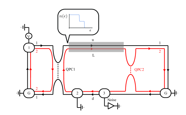
Figure 6: Schematic diagram of the device used to prepare an non-equilibrium state and probe its relaxation in the $\nu=2$ quantum Hall state of a 2D electron gas subject to a magnetic field.

VII.2 Mesoscopic systems

Despite being ultracold atomic gases a major motivation for the study of quantum quenches and non-equilibrium dynamics, it may appear as somewhat striking to some that, some of the above theoretical ideas have found faster applications in the realm of mesoscopic systems of electrons. However, when subjected to intense magnetic fields and low temperatures, the “dirty” 2D gases of interacting electrons in the quantum Hall regime have been for some time the arena for many experiments that have reached the precision standards of atomic physics in interferometryyang2002 , for instance.

Chirality arising from the application of the magnetic field makes the edges of the 2D electron gas in the integer quantum Hall regime behave as clean, non-interacting, conducting channels as far as the transport at small voltage bias is concerned. This is manifested in the perfect conductance quantization of the latter in units of $e^{2}/h$, which can be experimentally observed at low temperatures. However, this does not mean that the (screened) Coulomb interaction can be neglected. Coulomb interaction is indeed important to account for the spectral properties of the channels. Furthermore, its effect is especially felt when driving the system out of equilibrium. In this regard, Kovrizhin and Chalker chalker1 ; chalker2 first pointed out the interesting analogies between the study of the relaxation mechanisms of integer quantum Hall interferometers and the interaction quench in the LM. In this section, we shall closely follow the work of Milletarì and Rosenow milletari , which has also found recent experimental confirmation inue .

Using a Hall bar device like the one shown in Fig. 6 at Landau-level filling $\nu=2$, it is possible to prepare a double-step non-equilibrium distribution for the fermions in the outer edge channel (denoted by $1$ in Fig. 6). Mathematically,

$$n_{1R}(\epsilon)=a\theta(\mu_{1}-\epsilon)+(1-a)\theta(\mu_{2}-\epsilon),$$ (115)

where $\mu_{1}=(1-a)eV$ and $\mu_{2}=-aeV$ ($eV>0$), and $0<a<1$. The initial state corresponding to the above distribution is prepared by taking the outer channel $1$, which comes from a reservoir at chemical potential $eV$ through the first quantum point contact (QPC1). At this contact, the channel is brought in close contact with its grounded left-moving partner at the other edge of the Hall bar, which allows for local tunneling of electrons with different chemical potentials between the two. For non-interacting electrons, this results in the distribution function displayed in Eq. (115). After being driven out of equilibrium, channel $1$ is allowed to relax by interacting downstream with the grounded inner channel $2$ in the shaded region of Fig. 6. Chirality implies that time and space play the same role and the spatial overlap of the two channels in this region can be regarded as sudden quench of their mutual interaction. In the interaction region the channels are described by the (‘post-quench’) Hamiltonian:

$$H=\sum_{q>0}\left(a^{{\dagger}}_{1R}(q)\,a^{{\dagger}}_{2R}(q)\right)\left(\begin{array}[]{cc}v_{1}q&g_{4}q/2\\ g_{4}q/2&v_{2}q\end{array}\right)\left(\begin{array}[]{c}a_{1R}(q)\\ a_{2R}(q)\end{array}\right),$$ (116)

which can be diagonalized by means of the canonical transformation $a_{1R}(q)=\cos\theta\,b_{1R}(q)-\sin\theta\,b_{2R}(q)$ and $a_{2R}(q)=\sin\theta\,b_{1R}(q)+\cos\theta\,b_{2R}(q)$. The $\theta$ is the mixing angle, which is determined from $\tan 2\theta=\frac{g_{4}}{v_{1}-v_{2}}$, where $g_{4}$ parametrizes the (screened Coulomb) interaction between the two channels and $v_{1}$ and $v_{2}$ are the outer and inner channel velocities, respectively. Note that the appearance of trigonometric functions here (instead of the hyperbolic functions of the previous sections) is due to the same (right-moving) chirality of the two coupled fermionic channels. Nevertheless, as in the case of the LM, a solution of the quench dynamics can be obtained by means of the following time-dependent canonical transformation:

$$a_{1R}(q,t) =f_{1}(q,t)a_{1R}(q)+g(q,t)a_{2R}(q),$$ (117)

$$a_{2R}(q,t) =g(q,t)a_{1R}(q)+f_{2}(q,t)a_{2R}(q),$$ (118)

where

$$f_{1}(q,t) =\frac{1}{2}\left(e^{-i\tilde{v}_{1}qt}+e^{-i\tilde{v}_{2}qt}\right)+\frac{1}{2}\left(e^{-i\tilde{v}_{1}qt}-e^{-i\tilde{v}_{2}qt}\right)\cos 2\theta,$$ (119)

$$f_{2}(q,t) =\frac{1}{2}\left(e^{i\tilde{v}_{1}qt}+e^{i\tilde{v}_{2}qt}\right)-\frac{1}{2}\left(e^{i\tilde{v}_{1}qt}-e^{-i\tilde{v}_{2}qt}\right)\cos 2\theta,$$ (120)

$$g(q,t) =\frac{1}{2}\left(e^{-i\tilde{v}_{1}qt}-e^{-i\tilde{v}_{2}qt}\right)\sin 2\theta.$$ (121)

The parameters $\tilde{v}_{1(2)}=v_{1(2)}\cos^{2}\theta+v_{2(1)}\sin^{2}\theta\pm\frac{1}{2}g_{4}\sin 2\theta$ are the eigenmode velocities.

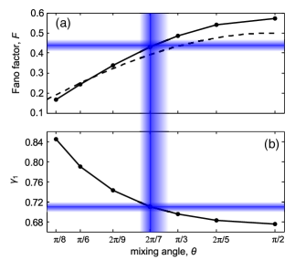
Figure 7: (a) Fano factor representing the fractional charge $e^{\star}=Fe$ in the inner channel $2$ (cf. Fig. 6) vs. the mixing angle $\theta$, which measures the strength of the inter-channel interaction. (b) Exponent $\gamma_{1}$ of the excess noise in the inner channel $2$ which is fitted acording to $\left[a(1-a)\right]^{\gamma_{1}}$, where $a$ is the transmission probability through the first quantum point contact (QPC1, see Fig. 6). The dots in both figures correspond to the numerical results obtained from the theory of Ref. milletari . The dashed line is a simple model proposed in Ref. inue , for which $F=(\sin\theta)/2$. The shaded (blue) area represents the best fit with the error of $1.2\sigma$ based on the fitted exponent $\gamma_{1}$.

After spatially overlapping, the two channels $1$ and $2$ are again spatially separated in order to probe the inner channel $2$ by taking it through a second quantum point contact at QPC2. There, it comes into contact with its left-moving partner before reaching ground together with outer channel (cf. Fig.  6). The shot noise in this channel is thus measured at contact number $3$  (cf. 6). Roughly speaking, shot noise measures the (fractional) charge of the carriers and can be obtained from the single-particle Green’s function of the channel ($\alpha=R,L$):

$$G^{<}_{2\alpha}(\tau)=\langle\psi^{{\dagger}}_{2\alpha}(x,t+\tau)\psi_{2\alpha}(x,t)\rangle.$$ (122)

through the expression:

$$S=\frac{2e^{2}}{\hbar}|t_{2}|^{2}\int d\epsilon\left[G^{<}_{2R}(\epsilon)G^{<}_{2L}(-\epsilon)+G^{<}_{2L}(\epsilon)G^{<}_{2R}(-\epsilon)\right]$$ (123)

where $t_{2}$ is the tunneling amplitude at the second point contact, QPC2. The Green’s function of the inner upstream channel can be written as follows:

$$G^{<}_{2R}(\tau) =G^{(0,<)}_{2R}(0,\tau)Z(x,t,\tau),$$ (124)

$$Z(x,t,\tau) =\langle e^{i\chi^{{\dagger}}(x,t,\tau)}e^{-i\chi(x,t,\tau)}\rangle,$$ (125)

$$G^{(0,<)}_{2R}(0,\tau) =\frac{1}{2\pi}\frac{1}{\left(-i\tilde{v}_{1}\tau+a_{0}\right)^{\sin^{2}\theta}\left(-i\tilde{v}_{2}\tau+a_{0}\right)^{\cos^{2}\theta}},$$ (126)

where $\chi(x,t,\tau)=\sum_{q>0}\left(\frac{2\pi}{qL}\right)^{1/2}e^{-qa_{0}/2}\>e^{iqx_{0}}\left[g(q,t+\tau)-g(q,t)\right]a_{1R}(q)$ and $a_{0}$ is a short-distance cut-off of the order of the magnetic length. The calculation of $Z(x,t,\tau)$ is complicated by non-gaussianity of the initial state, which yields the double-step distribution of Eq. (115). However, it can be still expressed in terms of a Fredholm determinant of the Toeplitz type and evaluated numerically milletari . The properties of the steady state are accessed by taking the limit $t\to+\infty$ in the above Green’s function. The resulting steady state is not thermal milletari , which is a consequence of the constrained dynamics of the model. The shot noise can be then extracted from the steady state Green’s function. The so-called Fano factor, corresponding to the ratio $F=S/S_{\mathrm{ref}}$ where $S_{\mathrm{ref}}=4epa(1-a)(e^{2}/h)V$ ($p=|t_{2}|^{2}\tilde{v}^{\sin^{2}\theta}_{1}\tilde{v}^{\cos^{2}\theta}_{2}$ is the reflection probability at the second quantum point contact milletari , and $V$ is the voltage bias), is shown in Fig. 7 as a function of the mixing angle, $\theta$. The experimental determination of its value (with the corresponding error bars) is indicated by the shaded (blue) region.

VIII Conclusions and outlook

Having the opportunity to write this article has taught us that the subject of quantum quenches in the Luttinger and related models continues to enjoy tremendous vitality after ten years. There are plenty of new analytical results, often obtained by the combination of powerful techniques which include conformal field theory, Bethe-ansatz, non-equilibrium (Keldysh) Green’s functions, etc. In addition, powerful numerical methods have been applied to various models and are teaching us where the analytics can be (and cannot be) applied.

Nevertheless, a deeper understanding of the universality of the LM predictions, beyond the rather fragmented knowledge obtained from specific models, is still lacking. In the authors’ view, such a framework still needs to be put in place. This framework should relate to some of the concepts of entanglement that have been surveyed in section V and should be able to account for the differences between gaussian and non-gaussian initial states. More importantly, the theoretical framework should also provide quantitative answers to questions about time scales and requirements for thermalization. It should tell which perturbations to the Hamiltonian of an exactly solvable model like Luttinger’s are dominant in driving the system towards thermal equilibrium, which ones subdominant, and what the time scales associated with them are.

On the experimental side, results are coming out at an increased pace. These include the recent observation of relaxation to the generalized Gibbs ensemble in an ultracold gas schmiedmayer . However, as theorists who cherish their own (theoretical) pets, we would like to see similar experiments carried out for a more faithful (fermionic) realization of the interaction quench in the Luttinger model. Our hope is that this article may motivate a young experimentalist to take on this challenge. In addition, let us mention that using different probes in the mesoscopic setup discussed in section VII.2 may allow for a more thorough characterization of the non-equilibrium steady state, and whether it is really a steady state or just a pre-thermalized one. Ultracold atomic systems still have a lot of offer as well as trapped ions iontraps since possibilities for the control of the system parameters and the preparation of the initial state are larger for these systems.

There are also new venues waiting to be fully explored. There is a zoo of newly discovered topologically-protected phases out there. Many of them are endowed with gapless states at their interfaces with topologically trivial matter. In two dimensions, some of these gapless states can be described as Tomonaga-Luttinger liquids, and the ideas described in section VII.2 can be relevant for the understanding of their non-equilibrium dynamics as well. From a broader perspective, we may also wonder what kind of new manifestations in the non-equilibrium dynamics of interacting system topological protection can bring in.

Going beyond isolated systems (or systems that can be treated to a large extent as such), the dynamics of the Luttiger model and its relatives coupled to environments is, to the best of our knowledge, a largely uncharted territory. The study of mesoscopic systems is clearly an area that can benefit from such studies since, in the solid state, it is much more difficult to completely isolate fragile quantum systems from their environment. Accounting for the effects of realistic sources of quantum dissipation cazalilladis is therefore an interesting research direction. Furthermore, in ultracold atomic systems, despite being largely isolated, it is also possible to engineer interesting environments eneko and the study of quantum dynamics in those setups should be a promising research topic.

- (1) M. Rigol and M. A. Cazalilla, New J. of Phys. 12, 055006 (2012).
- (2) A. Polkovnikov, K. Sengupta, A. Silva, and M. Vengalattore, Rev. Mod. Phys. 83 863 (2011).
- (3) J. Dziarmaga, Adv. in Phys. 59, 1063 (2010)
- (4) L. D’Alessio, Y. Kafri, A. Polkovnikov, and M. Rigol arxiv:1509.06411 (2015).
- (5) J. M. Luttinger, J. Math. Phys. 4, 1154 (1963).
- (6) D. C. Mattis and E. H. Lieb, J. Math. Phys. 6, 304 (1965).
- (7) P. Jordan, Z. Phys. 93 464 (1935); ibid 98, 795 (1936); ibid 99, 109 (1936); ibid 105, 114 (1937); ibid 105 229 (1937).
- (8) S. Tomonaga, Progr. Theor. Phys. (Kyoto) 5, 544 (1950).
- (9) J. Schwinger, Phys. Rev. Lett. 3, 296 (1959).
- (10) W. A. Little, Phys. Rev. 134, A1416 (1964).
- (11) A. Luther and V. J. Luther, Phys. Rev. Lett. 33, 589 (1974).
- (12) A. Luther and I. Peschel, Phys. Rev. B 12 3908, (1975).
- (13) F. D. M. Haldane, Phys. Rev. Lett. 45, 1358 (1980).
- (14) F. D. M. Haldane, J. of Phys. C 14, 2585 (1981).
- (15) F. D. M. Haldane, Phys. Rev. Lett. 47, 1840 (1981)
- (16) K. D. Schotte and U. Schotte, Phys. Rev. 182, 479 (1969); D. C. Mattis, J. Math. Phys. 15, 609 (1974); S. Mandelstam, Phys. Rev. D 11, 3026 (1975).
- (17) A. A. Gogolin, A. A. Nersesyan, and A. M. Tsvelik, Bosonization of Strongly Correlated Electrons, Cambridge (2002).
- (18) T. Giamarchi Quantum Physics in One Dimension (Oxford 2006).
- (19) M. Rigol, V. Dunjo, V. Yurovskii, and M. Olshanii, Phys. Rev. Lett. (2006).
- (20) T. Kinoshita, T. Wenger, and D. S. Weiss, Nature (London) 440, 900 (2006).
- (21) M. A. Cazalilla, Phys. Rev. Lett. 97 156403 (2006).
- (22) A. Mitra and T.Giamarchi, Phys. Rev. Lett. 107, 150602 (2011)
- (23) E. H. Lieb and D. Robinson, Commun. Math. Phys. 28, 251, (1972).
- (24) J. Cardy and P. Calabrese, Phys. Rev. Lett. 96, 136801 (2006).
- (25) A. Iucci and M. A. Cazalilla, Phys. Rev. A 80, 063619 (2009).
- (26) N. Nessi and A. Iucci, Physical Review B 87, 085137 (2013).
- (27) M. A. Cazalilla and J. B. Marston, Phys. Rev. Lett. 88, 256403 (2002); G. Vidal, Phys. Rev. Lett. 91 147902 (2003); S. R. White and A. E. Feiguin, Phys. Rev. Lett. 93, 076401 (2004); U. Schöllwock, Rev. Mod. Phys. 77, 259 (2005); U. Schöllwock, and S. R. White, Methods for Time Dependence in DMRG in G. G. Batrouni and D. Poilblanc (eds.) Effective models for low-dimensional strongly correlated systems, p. 155, AIP, Melville, New York (2006).
- (28) M. A. Cazalilla, J. Phys. B 37 S1 (2004).
- (29) R. Shankar, Rev. Mod. Phys. 66, 129 (1994).
- (30) See e.g. S. Sachdev, Quantum Phase Transitions, 2nd edition, Cambridge University Press (Cambridge, UK, 2011) and also Refs. bosonization_new ; giamarchi_book .
- (31) M. A. Cazalilla, R. Citro, T. Giamarchi, E. Orignac, and M. Rigol, Rev. Mod. Phys. 83, 1405 (2010).
- (32) C. Karrasch, J. Rentrop, D. Schuricht, V. Meden, Phys. Rev. Lett. 109, 126406 (2012).
- (33) M. Collura, P. Calabrese, and F. H. L. Essler, Phys. Rev. B 92, 125131 (2015).
- (34) J.Berges, S. Borsányi, and C. Wetterich, Phys.Rev. Lett. 93, 142002 (2004).
- (35) T. Kitagawa, A. Imambekov, J. Schmiedmayer, and E. Demler, New J. Phys. 13, 073018 (2011).
- (36) M. Gring, M. Kuhnert, T. Langen, T. Kitagawa, B. Rauer, M. Schreitl, I. Mazets, D. A. Smith, E. Demler, and J. Schmiedmayer, Science 337, 1318 (2012).
- (37) M. Moeckel and S. Kehrein, Phys. Rev. Lett. 100, 175702 (2008); Ann. Phys. (N. Y.) 324, 2146 (2009).
- (38) M. Eckstein, M. Kollar, and P. Werner, Phys. Rev. Lett. 103, 056403 (2009).
- (39) N. Nessi, A. Iucci, and M. A. Cazalilla, Phys. Rev. Lett. 113, 210402 (2014).
- (40) A. Houghton and J. B. Marston, Phys. Rev. B 48, 7790 (1993); A. Houghton, H.-J. Kwon, and J. B. Marston, Phys. Rev. B 50, 1351 (1994); A. Houghton, H.-J. Kwon, and J. B. Marston, Adv. Phys. 149, 141 (2000).
- (41) M.-C. Chung, A. Iucci, and M. A. Cazalilla, New J. Phys. 14, 075013 (2012).
- (42) A. Einstein, B. Podolsky and N. Rosen, Phys. Rev. 47, 777 (1935).
- (43) J. S. Bell Physics 1 (3): 195–200 (1964).
- (44) M. A. Nielsen and I. L. Chuang Quantum Computation and Quantum Information, Cambridge University Press (Cambridge, UK, 2000).
- (45) L. Amico, R. Fazio, A. Osterloh and V. Vedral, Rev. Mod. Phys. 80, 517 (2008).
- (46) A. Aspect, Ph. Grangier, and G. Roger, Phys. Rev. Lett. 49, 91 (1982).
- (47) I. Peschel, X. Wang, M Kaulke and K. Hallberg, Density-Matrix Renormalization, Springer
- (48) F. Verstraete, J. I. Cirac and V. Murg, Adv. Phys. 57,143 (2008).
- (49) G. Vidal, J. I. Latorre, E. Rico and A. Kitaev, Phys.Rev.Lett. 90, 227902,(2003)
- (50) A. Osterloh, L. Amico, G. Falci and R. Fazio, Nature, 416, 609 (2002)
- (51) H. Li and F. D. M. Haldane, Phys. Rev. Lett. 101, 010504 (2008).
- (52) M. Rigol, V. Dunjko, V. Yurovsky and M. Olshanii, Phys. Rev. Lett. 98 050405; M. Rigol M, A. Muramatsu and M. Olshanii, Phys. Rev. A 74, 053616 (2006)
- (53) M. A. Cazalilla, A. Iucci and M.-C. Chung, Phys. Rev. E 85, 011133 (2012)
- (54) C. H. Bennett, D. P. DiVincenzo, J. A. Smolin and W. K. Wooters, Phys. Rev. A 54, 3824 (1996)
- (55) J. Eisert, M. Cramer and M.B. Plenio, Rev. Mod. Phys. 82 (1). 277 (2010).
- (56) E. T. Jaynes, Phys. Rev. 106, 620 (1957);ibid 108, 171 (1957).
- (57) I. Peschel and V. Eisler, J. Phys. A: Math. Theor.42 504003 (2009)
- (58) M. Rigol, A. Muramatsu, and M. Olshanii, Phys. Rev. A 74, 053616 (2006).
- (59) A. C. Cassidy, C. W. Clark, Marcos Rigol, Phys. Rev. Lett. 106, 140405 (2011).
- (60) M. C. Chung and I. Peschel, Phys. Rev. B 64, 064412 (2001).
- (61) S.-A. Cheong and C. L. Henley, Phys. Rev. B 69, 075111 (2004); I. Peschel, J. Phys. A 36, L205 (2003); T. Barthel, M.-C. Chung, and U. Schollwöck, Phys. Rev. A 74, 022329 (2006).
- (62) B. Dora, M. Haque and G. Zaránd, Phys. Rev. Lett. 106, 156406 (2011)
- (63) B. Dora, F. Pollmann, J. Fortágh and G. Zaránd, Phys. Rev. Lett. 111, 046402 (2013)
- (64) P. W. Anderson, Phys. Rev. Lett. 18 1049 (1967).
- (65) F. Pollmann, S. Mukerjee, A. G. Green, and J. E. Moore, Phys. Rev. E 81, 020101 (2010).
- (66) J. O. Fjaerestad, J. Stat. Mech. P07011 (2008); M.-F. Yang, Phys. Rev. B 76, 180403 (2007).
- (67) J.-S. Bernier, R. Citro, C. Kollath and E. Orignac, Phys. Rev. Lett. 112, 065301 (2014).
- (68) J. Dziarmaga and M. Tylutki, Phys. Rev. E 84, 214522 (2011)
- (69) S. N. Dinh, D. A. Bagrets and A. D. Mirlin, Phys. Rev. B 88, 245405 (2013)
- (70) S. Sotiriadis, arXiv: 1507.07915 (2015).
- (71) K. Aikawa, A. Firsch, M. Mark, S. Baier, R. Grimm, and F. Ferlaino, Phys. Rev. Lett. 112, 010404 (2014); N. Q. Burdick, K. Baumann, Y. Tang, M. Lu, B. L. Lev, Phys. Rev. Lett. 114, 023201 (20125.
- (72) T. Langen et al. Science 348 207 (2015).
- (73) A. Iucci and M. A. Cazalilla, New J. Phys. 12 055019 (2010).
- (74) E. Dalla Torre, E. Demler, and A. Polkovnikov, Phys. Rev. Lett. 110, 090404 (2013)
- (75) L. Foini and T. Giamarchi, Phys. Rev. A 91, 023627 (2015).
- (76) C. De Grandi, V. Gritsev, and A. Polkovnikov, Phys. Rev. B 81, 224301 (2010).
- (77) M. Tezuka, A. García-García, and M. A. Cazalilla, Phys. Rev. A 90, 053618 (2014).
- (78) M. A. Cazalilla, F. Sols, and F. Guinea, Phys. Rev. Lett. 97, 076401 (2006).
- (79) A. M. Lobos, M. Tezuka, and A. M. García-García, Phys. Rev. B 88, 134506 (2013).
- (80) J. W. Britton, B. C. Sawyer, A. C. Keith, C.-C. J. Wang, J. K. Freericks, H. Uys, M. J. Biercuk, and J. J. Bollinger, Nature (London) 484, 489 (2012); R. Islam, C. Senko, W. C. Campbell, S. Korenblit, J. Smith, A. Lee, E. E. Edwards, C.-C. J. Wang, J. K. Freericks, and C. Monroe, Science 340, 583 (2013).
- (81) M. Rigol, Vanja Dunjko, and M. Olshanii, Nature (London) 452, 854 (2008).
- (82) M. Rigol, arXiv:1511.04447 (2015).
- (83) M. Buchhold, M. Heyl, and S. Diehl, report arxiv:1510.03447 (2015).
- (84) Y. Yang, Y. Chung, D. Sprinzak, M. Heiblum, D. Mahalu, and H. Shtrikman, Nature (London) 422, 415 (2002).
- (85) D. L. Kovrizhin and J. T. Chalker, Phys. Rev. B 84, 085105 (2011).
- (86) D. L. Kovrizhin and J. T. Chalker, Phys. Rev. Lett. 109, 106405 (2012).
- (87) M. Milletari and B. Rosenow, Phys. Rev. Lett. 111, 136807 (2013).
- (88) H. Inoue, A. Grivnin, N. Ofek, I. Neder, M. Heiblum, V. Umansky, and D. Mahalu, Phys. Rev. Lett. 112, 166801 (2014).
- (89) E. Malatsetxebarria, Z. Cai, U. Schollwöck, and M. A. Cazalilla, Phys. Rev. A 88, 063630 (2013); Z. Cai, U. Schöllwock, L. Pollet Phys. Rev. Lett. 113, 260403 (2014).